Asymptotic (statistical) periodicity in two-dimensional maps

Abstract

In this paper we give a new sufficient condition for asymptotic periodicity of Frobenius–Perron operator corresponding to two–dimensional maps. The result of the asymptotic periodicity for strictly expanding systems, that is, all eigenvalues of the system are greater than one, in a high-dimensional dynamical systems was already known. Our new theorem enables to apply for the system having an eigenvalue smaller than one. The key idea for the proof is a function of bounded variation defined by line integration. Finally, we introduce a new two-dimensional dynamical system exhibiting the asymptotic periodicity with different periods depending on parameter values, and discuss to apply our theorem to the model.

Fumihiko Nakamura

Kitami Institute of Technology,

165 Koen-cho, Kitami city, Hokkaido, 090-8507, Japan

Michael C. Mackey

McGill University,

3655 Promenade Sir William Osler, Montreal, Quebec H3G 1Y6, Canada

2020 Mathematics Subject Classification. Primary: 37A30, 26A45; Secondary: 37E30.

Key words and phrases. Asymptotic periodicity, bounded variation, Frobenius–Perron operator, two-dimensional map, Farey series.

1 Introduction

In examining the behaviour of dynamical systems, two main complementary threads have emerged. In one, the evolution of trajectories is the main focus, while in the other the evolution of densities is considered. In the latter case, one can think of the evolution of densities representing the overall statistical behaviour when a large (‘infinite’) number of trajectories are examined. In this paper we focus on the second point of view, which is closely related to early work in statistical physics initiated by both Boltzmann [1] and Gibbs [2] over a century ago and which forms the basis of the field of ergodic theory.

In examining the evolution of densities, there are three major types of behaviour that may occur and they are ergodicity, mixing, and exactness [3]. In addition there is a less well known fourth type of behaviour, called asymptotic periodicity (or statistical periodicity), which was first introduced and studied by Keller [4]. We will say more about these four types of behaviour in Section 2.

Asymptotic periodicity is known to occur in deterministic discrete time dynamical systems [5, 6, 7, 8] as well as being induced by noise [9, 10, 11]. One example of asymptotic periodicity in a deterministic setting is that of the hat (or tent) map

$$x_{n+1}=\left\{\begin{array}[]{ll}ax_{n}&x_{n}\in[0,\frac{1}{2}]\\ a(1-x_{n})&x_{n}\in(\frac{1}{2},1],\end{array}\right.$$ (1)

which was considered by Ito [12, 13], Shigematsu [14], and Yoshida [15] initially and then by Provatas [8] within the framework of asymptotic periodicity. To our knowledge the only studies of noise induced asymptotic periodicity are in the noise perturbed Nagumo-Sato [16] map (also known as the Keener [17] map) and given by

$$x_{n+1}=\alpha x_{n}+\beta+\xi_{n}\qquad\mbox{mod}\ 1$$ (2)

where $0<\alpha,\beta<1$ and the $\{\xi_{n}\}$ are independent random variables distributed with a density $g$, and studied by [9, 10, 11].

In this paper we present a new theorem on asymptotic periodicity in maps of dimension greater than one, extending the result of [18] for asymptotic periodicity in a high-dimensional dynamical systems which was stated for strictly expanding systems, that is, for systems in which all eigenvalues are greater than one.

In Section 2.1 we summarize some elementary concepts and tools from ergodic theory, and then in Section 2.2 give some background and simple results on bounded variation for functions of two variables that will be essential in the proof of our main Theorem 3.1 in Section 3. In Section 4 we consider an example of our main theorem and illustrate how the period changes as parameters are changed.

2 Background

2.1 Tools and definitions from ergodic theory

This section collects together some basic concepts needed later. Consult [3] for more details.

Let $(X,\mathcal{A},\mu)$ be a measure space and assume that a system has states distributed in a phase space $X$, and that the distribution of these states is characterized by a time dependent density $f_{n}(x)$, $n\in\mathbb{N}$. Remember that $f$ is a density if $f(x)\geq 0,\ \int_{X}f(x)\,d\mu(x)=1$. Equilibrium is characterized by a time independent density $f_{*}(x)$. Given a phase space $X$ we will denote the space of all densities on $X$ by $D(X)$ or by $D$ if $X$ is understood.

Also think of a dynamics $S$ operating on the same phase space $X$, $S:X\rightarrow X$. One way to think about a dynamics is through the evolution of a trajectory emanating from a single initial condition in the phase space $X$, and a complementary approach is to study how a density of initial conditions evolves under the action of the dynamics. With a dynamics $S$ and initial density $f_{0}(x)$ of states, the evolution of the density $f_{n}(x)$ is given by $f_{n}(x)=P_{S}^{n}f_{0}(x)$, wherein $P_{S}$ is the Markov (or evolution transfer) operator corresponding to $S$.

Definition 2.1.

Any operator $P:L^{1}(X)\rightarrow L^{1}(X)$ that satisfies

$$Pf\geq 0\quad\text{and}\quad\lVert Pf\rVert_{L^{1}}=\lVert f\rVert_{L^{1}}$$

for any $f\geq 0$, $f\in L^{1}(X)$ is called a Markov (or evolution) operator. If we restrict ourselves to only considering densities $f$, then any operator $P$ which when acting on a density again yields a density is a density evolution operator.

Given an evolution operator $P$ operating on densities alone, so $P:D\to D$, if there is a density $f_{*}$ such that $Pf_{*}=f_{*}$ then $f_{*}$ is called a stationary density.

Definition 2.2.

Let $(X,{\mathcal{A}},\mu)$ be a measure space . If $S$ is a nonsingular transformation, then the unique Markov operator $P:L^{1}(X)\rightarrow L^{1}(X)$ defined by

$$\int_{A}Pf(x)\,d\mu(x)=\int_{S^{-1}(A)}f(x)\,d\mu(x)$$ (3)

is called the Frobenius-Perron operator corresponding to $S$.

Definition 2.3.

Let $(X,{\mathcal{A}},\mu)$ be a measure space and let a nonsingular transformation $S\colon X\rightarrow X$ be given. Then $S$ is called ergodic if every invariant set $A\in{\mathcal{A}}$ (i.e. $S^{-1}(A)=A$) is such that either $\mu(A)=0$ or $\mu(X\setminus A)=0$; that is, $S$ is ergodic if all invariant sets are trivial subsets of $X$.

Ergodicity is equivalent to:

Theorem 2.4.

[3, Theorem 4.4.1a] Let $(X,{\mathcal{A}},\mu)$ be a normalized measure space, $\mu(X)=1$. A dynamics $S$ on a phase space $X$ with Frobenius-Perron operator $P_{S}$ and unique stationary density $f_{*}$ is ergodic if and only if $\{P^{n}f_{0}\}$ is Cesàro convergent to $f_{*}$ for all initial densities $f_{0}$, i.e., if

$$\lim_{n\to\infty}\frac{1}{n}\sum_{k=0}^{n-1}<P^{k}f_{0},g>=<f_{*},g>$$ (4)

where $g$ is any bounded measurable function and

$$<f,g>=\int_{X}f(x)g(x)d\mu(x)$$ (5)

denotes the $\mathbb{R}$-valued inner product.

Definition 2.5.

Let $(X,{\mathcal{A}},\mu)$ be a normalized measure space, and $S\colon X\rightarrow X$ a measure-preserving transformation. $S$ is called mixing if

$$\lim_{n\rightarrow\infty}\mu(A\cap S^{-n}(B))=\mu(A)\mu(B)\qquad\mbox{for all }A,B\in{\mathcal{A}}.$$ (6)

Mixing implies ergodicity and is equivalent to:

Theorem 2.6.

[3, Theorem 4.4.1b] A dynamics $S$ on a phase space $X$ with Frobenius-Perron operator $P_{S}$ and unique stationary density $f_{*}$ is mixing if and only if

$$\lim_{n\to\infty}<P_{S}^{n}f_{0},g>=<f_{*},g>,$$ (7)

for every initial density $f_{0}\in\mathcal{D}$ and bounded measurable function $g$.

Definition 2.7.

Let $(X,{\mathcal{A}},\mu)$ be a normalized measure space and $S\colon X\rightarrow X$ a measure-preserving transformation such that $S(A)\in{\mathcal{A}}$ for each $A\in{\mathcal{A}}$. If

$$\lim_{n\rightarrow\infty}\mu(S^{n}(A))=1\qquad\mbox{for every }A\in{\mathcal{A}},\mu(A)>0,$$ (8)

then $S$ is called exact or asymptotically stable.

Exactness implies mixing and is equivalent to:

Theorem 2.8.

[3, Theorem 4.4.1c] A dynamics $S$ on a phase space $X$ with Frobenius-Perron operator $P_{S}$ and unique stationary density $f_{*}$ is asymptotically stable if and only if

$$\lim_{n\to\infty}||P_{S}^{n}f-f_{*}||_{L^{1}}=0$$ (9)

for every initial density $f\in D$.

Asymptotically stable systems have a number of interesting properties (cf. [3, 19] for more complete details). Asymptotically stable systems are non-invertible and they always have a unique stationary density $f_{*}$.

Next, we define a smoothing Markov operator.

Definition 2.9.

Let $(X,\mathcal{A},\mu)$ be a measure space. A Markov operator $P$ is said to be smoothing (or constrictive) if there exists a set $A$ of finite measure, and two positive constants $k<1$ and $\delta>0$ such that for every set $E$ with $\mu(E)<\delta$ and every density $f$ there is some integer $n_{0}(f,E)$ for which

$$\int_{E\cup(X\setminus A)}P^{n}f(x)\,d\mu(x)\leq k\qquad\text{for }n\geq n_{0}(f,E).$$

This definition of smoothing just means that any initial density, even if concentrated on a small region of the phase space $X$, will eventually be ’smoothed’ out by $P^{n}$ and not end up looking like a delta function. Notice that if $X$ is a finite phase space we can take $X=A$ so the smoothing condition looks simpler:

$$\int_{E}P^{n}f(x)\,d\mu(x)\leq k\qquad\text{for }n\geq n_{0}(f,E).$$

Smoothing operators are important because of a theorem of [20] introduced next, first proved in a more restricted situation by [5]. Although the property called weakly constrictive introduced in [5] and [20] seems to be different from smoothing, it also leads to asymptotic periodicity. Conversely, we can immediately show that an asymptotically periodic Markov operator is smoothing and weakly constrictive in the sense of [5]. Thus we conclude smoothing and weakly constrictiveness are equivalent.

Theorem 2.10 (Spectral Decomposition Theorem, [20]).

Let $P$ be a smoothing Markov operator. Then there is an integer $r>0$, a sequence of nonnegative densities $g_{i}$ and a sequence of bounded linear functionals $\lambda_{i}$, $i=1,\ldots,r,$ and an operator $Q:L^{1}(X)\rightarrow L^{1}(X)$ such that for all densities $f$, $Pf$ has the form

$$Pf(x)=\sum_{i=1}^{r}\lambda_{i}(f)g_{i}(x)+Qf(x).$$ (10)

The densities $g_{i}$ and the transient operator $Q$ have the following properties:

1. The $g_{i}$ have disjoint support (i.e. are mutually orthogonal and thus form a basis set), so $g_{i}(x)g_{j}(x)=0$ for all $i\neq j$.

2. For each integer $i$ there is a unique integer $\alpha(i)$ such that $Pg_{i}=g_{\alpha(i)}$. Furthermore, $\alpha(i)\neq\alpha(j)$ for $i\neq j$. Thus the operator $P$ permutes the densities $g_{i}$.

3. $\parallel P^{n}Qf\parallel\rightarrow 0$ as $n\rightarrow\infty,\qquad n\in\mathbb{N}$.

Notice from (10) that $P^{n+1}f$ may be immediately written in the form

$$P^{n+1}f(x)=\sum_{i=1}^{r}\lambda_{i}(f)g_{\alpha^{t}(i)}(x)+Q_{n}f(x),\qquad n\in\mathbb{N}$$ (11)

where $Q_{n}=P^{n}Q$, $\parallel Q_{n}f\parallel\rightarrow 0$ as $n\rightarrow\infty$, and $\alpha^{n}(i)=\alpha(\alpha^{n-1}(i))=\cdots$. The density terms in the summation of (11) are just permuted by each application of $P$. Since $r$ is finite, the series

$$\sum_{i=1}^{r}\lambda_{i}(f)g_{\alpha^{t}(i)}(x)$$ (12)

must be periodic with a period $T\leq r!$. Further, as $\{\alpha^{n}(1),\ldots,\alpha^{n}(r)\}$ is just a permutation of ${1,\cdots,r}$ the summation (12) may be written in the alternative form

$$\sum_{i=1}^{r}\lambda_{\alpha^{-t}(i)}(f)g_{i}(x),$$

where $\alpha^{-n}(i)$ is the inverse permutation of $\alpha^{n}(i)$.

This rewriting of the summation portion of (11) makes the effect of successive applications of $P$ completely transparent. Each application of $P$ simply permutes the set of scaling coefficients associated with the densities $g_{i}(x)$ [remember that these densities have disjoint support].

Since $T$ is finite and the summation (12) is periodic (with a period bounded above by $r!$), and $\parallel Q_{n}f\parallel\rightarrow 0$ as $n\rightarrow\infty$, we say that for any smoothing Markov operator the sequence $\{P^{n}f\}$ is asymptotically (statistically) periodic or, more briefly, that $P$ is asymptotically periodic. Komorník [21] has reviewed the subject of asymptotic periodicity.

Asymptotically periodic Markov operators always have at least one stationary density given by

$$f_{*}(x)=\dfrac{1}{r}\sum_{i=1}^{r}g_{i}(x),$$ (13)

where $r$ and the $g_{i}(x)$ are defined in Theorem 2.10. It is easy to see that $f_{*}(x)$ is a stationary density, since by Property 2 of Theorem 2.10 we also have

$$Pf_{*}(x)=\dfrac{1}{r}\sum_{i=1}^{r}g_{\alpha(i)}(x),$$

and thus $f_{*}$ is a stationary density of $P^{n}$. Hence, for any smoothing Markov operator the stationary density (13) is just the average of the densities $g_{i}$.

Remark 2.11.

It is known [3, Section 5.5] that mixing, exactness and asymptotically periodicity with $r=1$ are all equivalent for a smoothing Markov operator. This means that the case $r=1$ has a strictly stronger mixing property than the case $r>1$. In terms of published examples having periodicity with not only $r=1$ but also $r>1$, we only know the hat map (1) and the noise perturbed [16] map (2) (see section 4 for a discussion of the parameters of the hat map showing asymptotic periodicity when $r>1$). The model we introduce in Section 4 is a new two-dimensional example having different periods depending on parameter values.

2.2 Functions of bounded variation in two variables

There are many definitions of the total variation for functions of two real variables. For example, see [22] and [23] summarized in [24, 25]. In this paper, we refer to the definition in [26] which is defined using line integration.

Consider a compact subset $\sigma\subset\mathbb{R}^{2}$, a function $f:\sigma\to\mathbb{R}$ and a continuous and piecewise $C^{1}$ curve $\gamma:[0,1]\to\mathbb{R}^{2}$. Although Ashton [26] found it sufficient to consider polygonal curves, that is, piecewise linear continuous curves, we need to treat more general continuous curves since we focus on non-linear transformations. We denote the set of all continuous and piecewise $C^{1}$ curves by $\Gamma$.

Definition 2.12.

Let $\gamma\in\Gamma$, then $\{(x_{i},y_{i})\}_{i=1}^{n}$ is called a partition of $\gamma$ over $\sigma$ if $(x_{i},y_{i})\in\sigma$ for all $i$ and there exists a partition $\{s_{i}\}_{i=1}^{n}\in\Lambda([0,1])$ such that $(x_{i},y_{i})=\gamma(s_{i})$ for all $i$, where $\Lambda([0,1])$ is the set of all partitions of $[0,1]$. The set of all partitions of $\gamma$ over $\sigma$ is denoted by $\Lambda(\gamma,\sigma)$.

Definition 2.13.

Let $\sigma\subset\mathbb{R}^{2}$ be compact, and consider a function $f:\sigma\to\mathbb{R}$ and a curve $\gamma\in\Gamma$. The variation of $f$ along the curve $\gamma$ is defined as

$${\rm cvar}(f,\gamma,\sigma):=\sup_{\{(x_{j},y_{j})\}_{j=1}^{n}\in\Lambda(\gamma,\sigma)}\sum_{j=1}^{n-1}|f(x_{j+1},y_{j+1})-f(x_{j},y_{j})|.$$ (14)

Remark 2.14.

From the definition, one can rewrite ${\rm cvar}(f,\gamma,\sigma)$ as

$${\rm cvar}(f,\gamma,\sigma)=\sup_{\begin{subarray}{c}\{t_{j}\}_{j=1}^{n}\in\Lambda([0,1])\\ \gamma(t_{j})\in\sigma\end{subarray}}\sum_{j=1}^{n-1}|f\circ\gamma(t_{j+1})-f\circ\gamma(t_{j})|.$$ (15)

Note that we sometimes omit $\gamma(t_{j})\in\sigma$ and simply write $\displaystyle\sup_{\{t_{j}\}_{j=1}^{n}\in\Lambda([0,1])}$ for the above equation.

The following basic properties for the variation are known.

Proposition 2.15.

([26, Proposition 3.2]) Let $\sigma_{1}\subset\sigma$ be a nonempty compact subset of $\mathbb{R}^{2}$, $f,g:\sigma\to\mathbb{R}$, $\gamma\in\Gamma$ and $\alpha\in\mathbb{R}$. Suppose $\gamma=\gamma_{1}\circ\gamma_{2}\in\Gamma$ with $\gamma_{1}(1)\in\sigma$. Then,

• ${\rm cvar}(f+g,\gamma,\sigma)\leq{\rm cvar}(f,\gamma,\sigma)+{\rm cvar}(g,\gamma,\sigma)$,

• ${\rm cvar}(fg,\gamma,\sigma)\leq\|f\|_{\infty}{\rm cvar}(g,\gamma,\sigma)+\|g\|_{\infty}{\rm cvar}(f,\gamma,\sigma)$,

• ${\rm cvar}(\alpha f,\gamma,\sigma)=|\alpha|{\rm cvar}(f,\gamma,\sigma)$,

• ${\rm cvar}(g,\gamma,\sigma)={\rm cvar}(g,\gamma_{1},\sigma)+{\rm cvar}(g,\gamma_{2},\sigma)$,

• ${\rm cvar}(g,\gamma_{1},\sigma)\leq{\rm cvar}(g,\gamma,\sigma)$,

• ${\rm cvar}(g,\gamma,\sigma_{1})\leq{\rm cvar}(g,\gamma,\sigma)$.

Definition 2.16.

The compact and connected sets $\sigma_{1},\sigma_{2}$ are said to be adjacent if $\sigma_{1}\cap\sigma_{2}\neq\emptyset$ and $int(\sigma_{1}\cap\sigma_{2})=\emptyset$.

Now we note the following property for the ${\rm cvar}(f,\gamma,\sigma)$.

Proposition 2.17.

([27, Theorem 4.9]) Let $\sigma_{1},\sigma_{2}$ be two compact and connected adjacent sets. Then, for any $f:\sigma_{1}\cup\sigma_{2}\to\mathbb{R}$,

$${\rm cvar}(f,\gamma,\sigma_{1}\cup\sigma_{2})={\rm cvar}(f,\gamma,\sigma_{1})+{\rm cvar}(f,\gamma,\sigma_{2}).$$

Lemma 2.18.

Let $\sigma_{1}\subset\sigma$ be a nonempty compact on $\mathbb{R}^{2}$, $f:\sigma\to\mathbb{R}$ and $\gamma\in\Gamma$. Assume that $g:\sigma_{1}\to g(\sigma_{1})$ is a one-to-one map. Then,

$${\rm cvar}(f\circ g,\gamma,\sigma_{1})={\rm cvar}(f,g\circ\gamma,g(\sigma_{1}))$$

Proof.

$${\rm cvar}(f\circ g,\gamma,\sigma_{1}) = \sup_{\begin{subarray}{c}\{t_{j}\}_{j=1}^{n}\in\Lambda([0,1])\\ \gamma(t_{j})\in\sigma_{1}\end{subarray}}\sum_{j=1}^{n-1}|f\circ g(\gamma(t_{j+1}))-f\circ g(\gamma(t_{j}))|$$

$$= \sup_{\begin{subarray}{c}\{t_{j}\}_{j=1}^{n}\in\Lambda([0,1])\\ g\circ\gamma(t_{j})\in g(\sigma_{1})\end{subarray}}\sum_{j=1}^{n-1}|f(g\circ\gamma(t_{j+1}))-f(g\circ\gamma(t_{j}))|$$

$$= {\rm cvar}(f,g\circ\gamma,g(\sigma_{1}))$$

∎

Definition 2.19.

Let $\mathcal{C}$ be the set of all convex closed Jordan curve on $\mathbb{R}^{2}$. Then $t\in[0,1]$ is said to be an entry point of $\gamma\in\Gamma$ on a curve $c\in\mathcal{C}$ if either

• $t=0$ and $\gamma(0)\in c$, or

• $\gamma(t)\in c$ and for all $\varepsilon>0$ there exists $s\in(t-\varepsilon,t)\cap[0,1]$ such that $\gamma(s)\notin c$.

Set ${\rm vf}(\gamma,c)$ to be the number of entry points of $\gamma$ on $c\in\mathcal{C}$ and ${\rm vf}(\gamma)$ to be the supremum of ${\rm vf}(\gamma,c)$ over all convex closed Jordan curves $c$, that is,

$${\rm vf}(\gamma):=\sup_{c\in\mathcal{C}}{\rm vf}(\gamma,c).$$ (16)

Remark 2.20.

In [26], ${\rm vf}(\gamma,c)$ is defined by lines instead of curves, but we need the definition by curves for our main theorem.

Definition 2.21.

Let $f:\sigma\to\mathbb{R}$. The variation of $f$ on $\sigma$ is defined by

$${\rm Var}(f,\sigma):=\sup_{\gamma\in\Gamma}\frac{{\rm cvar}(f,\gamma,\sigma)}{{\rm vf}(\gamma)}.$$ (17)

If $\gamma\in\Gamma$ satisfies ${\rm vf}(\gamma)=\infty$ and ${\rm cvar}(f,\gamma,\sigma)=\infty$, then we define ${\rm cvar}(f,\gamma,\sigma)/{\rm vf}(\gamma)=0$.

The following properties for the variation define above are well-known.

Proposition 2.22.

Let $\sigma_{1}\subset\sigma$ be a nonempty compact subset of $\mathbb{R}^{2}$, $f,g:\sigma\to\mathbb{R}$ and $\alpha\in\mathbb{R}$. Then,

• ${\rm Var}(f+g,\sigma)\leq{\rm Var}(f,\sigma)+{\rm Var}(g,\sigma)$,

• ${\rm Var}(fg,\sigma)\leq\|f\|_{\infty}{\rm Var}(g,\sigma)+\|g\|_{\infty}{\rm Var}(f,\sigma)$,

• ${\rm Var}(\alpha f,\sigma)=|\alpha|{\rm Var}(f,\sigma)$,

• ${\rm Var}(f,\sigma_{1})\leq{\rm Var}(f,\sigma)$.

Proof.

The proof of all properties follows immediately from Proposition 2.15. See also [26]. ∎

Finally, we state and prove the following lemma in order to prove our main theorem.

Lemma 2.23.

Let $\sigma\subset\mathbb{R}^{2}$ be a compact set. Assume $g:\mathbb{R}^{2}\to\mathbb{R}$ is a $C^{1}$ function. If there exists a constant $C>0$ such that $|g_{x}(x,y)|\leq C$ and $|g_{y}(x,y)|\leq C$ for any $(x,y\in Int(\sigma))$, then ${\rm Var}(g,\sigma)$ is bounded.

Proof.

$$\frac{{\rm cvar}(g,\gamma,\sigma)}{{\rm vf}(\gamma)} = \frac{1}{{\rm vf}(\gamma)}\sup_{\{(x_{i},y_{i})\}_{j=1}^{n}\in\Lambda(\gamma,\sigma)}\sum_{j=1}^{n-1}|g((x_{j+1},y_{j+1})-g(x_{j},y_{j})|$$

$$= \frac{1}{{\rm vf}(\gamma)}\sup_{\{(t_{i})\}_{j=1}^{n}\in\Lambda([0,1])}\sum_{j=1}^{n-1}|g\circ\gamma(t_{j+1})-g\circ\gamma(t_{j})|.$$

Since $g$ is a $C^{1}$ function and $\gamma$ is a piecewise $C^{1}$ curve, then we have

$$\leq \frac{1}{{\rm vf}(\gamma)}\int_{0}^{1}|(g\circ\gamma)^{\prime}(t)|dt$$

$$= \frac{1}{{\rm vf}(\gamma)}\int_{\gamma}|(g_{x}(x,y)\frac{dx}{dt}+g_{y}(x,y)\frac{dy}{dt})|dt$$

$$= \frac{1}{{\rm vf}(\gamma)}\int_{\gamma}|g_{x}(x,y)||dx|+|g_{y}(x,y)||dy|$$

$$\leq \frac{C}{{\rm vf}(\gamma)}\int_{\gamma}(|dx|+|dy|)$$

$$\leq \frac{C}{{\rm vf}(\gamma)}\int_{0}^{1}|\gamma^{\prime}(t)||dt|$$

$$\leq C{\rm Var}(x+y,\sigma),$$

which is bounded. Thus ${\rm Var}(g,\sigma)$ is bounded. ∎

3 Main theorem

Gora and Boyarsky [18] gave a sufficient condition for asymptotic (statistical) periodicity in piecewise $C^{2}$ maps on $\mathbb{R}^{N}$ using a general definition of the total variation. Their assumptions are stronger than ours since they assume that the map is expanding in all directions and thus all eigenvalues of the Jacobian are larger than one.

Our main result gives a sufficient condition for asymptotic periodicity of more general piecewise $C^{2}$ maps on $\mathbb{R}^{2}$, that are not necessarily expanding in all directions, by using the definition of variation constructed by line integration as introduced in [27]. Let $X\subset\mathbb{R}^{2}$ be a connected compact subset.

Theorem 3.1.

Let $S:X\to X$ satisfy the following conditions:

• There is a partition $I_{1},I_{2},\cdots,I_{r}$ of $X$ such that for each $i=1,\cdots,r$,

  • the restricted map $S|_{int(I_{i})}$ is a $C^{2}$ and one-to-one function,

  • each boundary $\partial(I_{i})$ is a piecewise $C^{2}$ curve having a finite boundary length,

  • the set $S(I_{i})$ is convex;

• For $i=1,\cdots,r$, each Jacobian $J_{i}(x,y)$ of $S|_{int(I_{i})}$ satisfies

  $$J_{i}(x,y)\geq\lambda>1\ \ \ {\it for}\ \ (x,y)\in int(I_{i});$$

• There are real constants $C^{\prime}>0$ such that, for $i=1,\cdots,r$,

  $$\left|\frac{\partial}{\partial x}J_{i}^{-1}(x,y)\right|\leq C^{\prime}<\infty,\ \ \ {\it for}\ \ (x,y)\in int(I_{i}),$$

  $$\left|\frac{\partial}{\partial y}J_{i}^{-1}(x,y)\right|\leq C^{\prime}<\infty,\ \ \ {\it for}\ \ (x,y)\in int(I_{i});$$

• There exists $C>0$ such that for any curves $\gamma$ on $X$, a curve $\widetilde{\gamma}$ constructed by connecting all curves $\{S|_{int(I_{i})}^{-1}(\gamma)\}_{i=1}^{r}$ whose length is minimal satisfies

  $$\sup_{\gamma\in\Gamma}\frac{{\rm vf}(\widetilde{\gamma})}{{\rm vf}(\gamma)}\leq C;$$

• The numbers $\lambda,C$ satisfy

  $$\frac{C}{\lambda}<1.$$

Let $P$ be the Frobenius-Perron operator corresponding to $S$. Then, for all $f\in D(X)$, $\{P^{n}f\}$ is asymptotically periodic.

Remark 3.2.

Item (ii) implies an area expanding property. If the system satisfied only condition (ii), we can immediately find a counterexample of non-asymptotically periodic transformations. For example, the piecewise linear map $S(x,y)=(4x,y/2)$ mod 1 has Jacobian $\lambda=2$ but has eigenvalues $4$ and $1/2$. It is clear that the map has no absolutely continuous invariant measure with respect to Lebesgue measure, which means that the corresponding Frobenius-Perron operator is not asymptotically periodic. However, if we take a partition satisfying (i) and the system satisfies (iv) and (v), then such counterexamples can be excluded. Indeed, we find that the factor $\frac{{\rm vf}(\widetilde{\gamma})}{{\rm vf}(\gamma)}$ must be larger than $\lambda$ for the map $S$, and (v) cannot hold.

Proof of Theorem 3.1

First we write the Frobenius-Perron operator $P$ corresponding to $S$ as

$$Pf(x,y)=\sum_{i=1}^{r}\rho_{i}(x,y)f(g_{i}(x,y))1_{I^{\prime}_{i}}(x,y),$$

where $g_{i}(x,y)=S_{i}^{-1}(x,y)$ and $\rho_{i}(x,y)=J_{i}^{-1}(x,y)$ for $(x,y)\in I^{\prime}_{i}$ with $I^{\prime}_{i}=S(I_{i})$ and $i=1,\cdots,r$. Each $J_{i}(x,y)$ is a Jacobian on $I^{\prime}_{i}$.

We then calculate the variation ${\rm Var}(Pf,X)$ for $f\in D(X)$ of bounded variation, denoted by $\underset{X}{\rm Var}(Pf)$. We first calculate, by (i) of Proposition 2.15,

$$\underset{X}{\rm Var}(Pf) = \sup_{\gamma\in\Gamma}\frac{1}{{\rm vf}(\gamma)}{\rm cvar}\left(\sum_{i=1}^{r}\rho_{i}(x,y)f(g_{i}(x,y))1_{I^{\prime}_{i}}(x,y),\gamma,X\right)$$

$$\leq \sup_{\gamma\in\Gamma}\frac{1}{{\rm vf}(\gamma)}\sum_{i=1}^{r}{\rm cvar}\left(\rho_{i}(x,y)f(g_{i}(x,y))1_{I^{\prime}_{i}}(x,y),\gamma,X\right)$$

By (ii) of Proposition 2.15,

$${\rm cvar}\left(\rho_{i}(x,y)f(g_{i})\cdot 1_{I^{\prime}_{i}},\gamma,X\right) \leq (\sup_{I^{\prime}_{i}}\rho_{i}){\rm cvar}\left(f\circ g_{i}\cdot 1_{I^{\prime}_{i}},\gamma,X\right)+{\rm cvar}\left(\rho_{i},\gamma,X\right)\sup_{I^{\prime}_{i}}f(g_{i})$$

$$\leq \frac{1}{\lambda}{\rm cvar}\left(f\circ g_{i}\cdot 1_{I^{\prime}_{i}},\gamma,X\right)+{\rm cvar}\left(\rho_{i},\gamma,X\right)\sup_{I^{\prime}_{i}}f(g_{i}).$$

By the mean value theorem for definite integrals, we have

$$\sup_{I^{\prime}_{i}}f(g_{i})\leq\frac{1}{\iint_{I^{\prime}_{i}}dxdy}\iint_{I^{\prime}_{i}}|f(g_{i}(x,y))|dxdy.$$ (18)

Then we have

$$\underset{X}{\rm Var}(Pf) \leq \sup_{\gamma\in\Gamma}\frac{1}{{\rm vf}(\gamma)}\left\{\frac{1}{\lambda}\sum_{i=1}^{r}{\rm cvar}(f\circ g_{i}\cdot 1_{I^{\prime}_{i}},\gamma,X)+\sum_{i=1}^{r}\frac{{\rm cvar}\left(\rho_{i},\gamma,X\right)}{\iint_{I^{\prime}_{i}}dxdy}\iint_{I^{\prime}_{i}}|f(g_{i}(x,y))|dxdy\right\}.$$ (20)

$$\leq \frac{1}{\lambda}\sup_{\gamma\in\Gamma}\frac{1}{{\rm vf}(\gamma)}\sum_{i=1}^{r}{\rm cvar}(f\circ g_{i}\cdot 1_{I^{\prime}_{i}},\gamma,X)$$

$$+\sup_{\gamma\in\Gamma}\frac{1}{{\rm vf}(\gamma)}\sum_{i=1}^{r}\frac{{\rm cvar}\left(\rho_{i},\gamma,X\right)}{\iint_{I^{\prime}_{i}}dxdy}\iint_{I^{\prime}_{i}}|f(g_{i}(x,y))|dxdy.$$

Since $\underset{X}{\rm Var}(\rho_{i})$ is bounded by Lemma 2.23, there is some constant $\hat{C}$ such that

$$\eqref{eq3-2}\leq\sum_{i=1}^{r}\frac{\hat{C}}{\iint_{I^{\prime}_{i}}dxdy}\iint_{I^{\prime}_{i}}|f(g_{i}(x,y))|dxdy.$$

Changing the variables by $g_{i}(x,y)=(\hat{x},\hat{y})$,

$$\leq\sum_{i=1}^{r}\frac{\hat{C}}{\iint_{I^{\prime}_{i}}dxdy}\iint_{I_{i}}f(\hat{x},\hat{y})d\hat{x}d\hat{y}\leq\max_{i}\frac{r\hat{C}}{\iint_{I^{\prime}_{i}}dxdy}$$ (21)

since $f\in D(X)$. We next calculate Eq.(20). For $i=1,\cdots,r$, $\{\gamma(t_{j})\}_{j=0}^{n-1}\subset X$, the sets $A_{i},B_{i},C_{i}$ are defined by

$$A_{i} := \{j=0,\cdots,n-1\ :\ \gamma(t_{j})\in I_{i}^{\prime}\quad{\rm and}\quad\gamma(t_{j+1})\in I_{i}^{\prime}\},$$

$$B_{i} := \{j=0,\cdots,n-1\ :\ {\rm either}\quad\gamma(t_{j})\notin I_{i}^{\prime}\quad{\rm or}\quad\gamma(t_{j+1})\notin I_{i}^{\prime}\},$$

$$C_{i} := \{j=0,\cdots,n-1\ :\ \gamma(t_{j})\notin I_{i}^{\prime}\quad{\rm and}\quad\gamma(t_{j+1})\notin I_{i}^{\prime}\}.$$

Then,

$${\rm cvar}(f\circ g_{i}\cdot 1_{I^{\prime}_{i}},\gamma,X) \leq \sum_{j\in A_{i}}|f\circ g_{i}(\gamma(t_{j+1})-f\circ g_{i}(\gamma(t_{j})|$$ (23)

$$+\sum_{j\in B_{I}}|\max\{f\circ g_{i}(\gamma(t_{j+1}),f\circ g_{i}(\gamma(t_{j})\}|.$$

By definition, we have

$$\eqref{eq4-1}\leq{\rm cvar}(f\circ g_{i},\gamma,I^{\prime}_{i}),$$

and

$$\eqref{eq3-1}\leq\frac{1}{\lambda}\sup_{\gamma\in\Gamma}\frac{1}{{\rm vf}(\gamma)}\sum_{i=1}^{r}{\rm cvar}(f\circ g_{i},\gamma,I^{\prime}_{i})+\frac{1}{\lambda}\sum_{i=1}^{r}\sup_{I^{\prime}_{i}}\left(f\circ g_{i}\right)\sup_{\gamma\in\Gamma}\frac{1}{{\rm vf}(\gamma)}\#\{j\in B_{i}\}.$$

Now let $\#\{j\in B_{i}\}$ be $m\leq n$. For this case ${\rm vf}(\gamma)$ must be larger than $m$ since $I^{\prime}_{i}$ is a convex closed Jordan curve by assumption (i). Thus we have

$$\eqref{eq3-1}\leq\frac{1}{\lambda}\sup_{\gamma\in\Gamma}\frac{1}{{\rm vf}(\gamma)}\sum_{i=1}^{r}{\rm cvar}(f\circ g_{i},\gamma,I^{\prime}_{i})+\frac{1}{\lambda}\sum_{i=1}^{r}\sup_{I^{\prime}_{i}}\left(f\circ g_{i}\right).$$ (24)

Using Lemma 2.18,

$$\sum_{i=1}^{r}{\rm cvar}(f\circ g_{i},\gamma,I^{\prime}_{i}) = \sum_{i=1}^{r}{\rm cvar}(f,g_{i}\circ\gamma,I_{i}).$$

Since $g_{i}\circ\gamma$ is a curve on $I_{i}$, we can make a new curve $\widetilde{\gamma}$ on $X$ by connecting all curves $g_{i}\circ\gamma$ for $i=1,\cdots,r$ whose length becomes minimal. Then, by (v) in Proposition 2.15,

$$\sum_{i=1}^{r}{\rm cvar}(f,g_{i}\circ\gamma,I_{i})\leq\sum_{i=1}^{r}{\rm cvar}(f,\widetilde{\gamma},I_{i}).$$

Moreover, since $\{I_{i}\}_{i=1}^{r}$ are adjacent, by Proposition 2.17,

$$\sum_{i=1}^{r}{\rm cvar}(f,\widetilde{\gamma},I_{i})={\rm cvar}(f,\widetilde{\gamma},X).$$ (25)

Thus, by assumption (iv),

$$\underset{X}{\rm Var}(Pf) \leq \frac{1}{\lambda}\sup_{\gamma\in\Gamma}\frac{{\rm vf}(\widetilde{\gamma})}{{\rm vf}(\gamma)}\frac{1}{{\rm vf}(\widetilde{\gamma})}{\rm cvar}(f,\widetilde{\gamma},X)+\max_{i}\frac{r(\hat{C}+1)}{\iint_{I^{\prime}_{i}}dxdy}$$ (26)

$$= \frac{C}{\lambda}\sum_{i=1}^{r}\underset{X}{\rm Var}(f)+L,$$

where

$$L:=\max_{i}\frac{r(\hat{C}+1)}{\iint_{I^{\prime}_{i}}dxdy}$$

is independent of $f$. Here we use the same procedure for the second term of Eq.(24) as in the calculations from Eq.(18) to Eq.(21). By assumption (v),

$$\underset{X}{\rm Var}(P^{n}f) \leq \left(\frac{C}{\lambda}\right)^{n}\underset{X}{\rm Var}(f)+L\sum_{j=0}^{n-1}\left(\frac{C}{\lambda}\right)^{j}$$

$$< \left(\frac{C}{\lambda}\right)^{n}\underset{X}{\rm Var}(f)+\frac{\lambda L}{\lambda-C},$$

and therefore, for every $f\in D(X)$ of bounded variation,

$$\lim_{n\to\infty}\sup\underset{X}{\rm Var}(P^{n}f)<K,$$

where $K>\lambda L/(\lambda-C)$ is independent of $f$. Hence, we define $\mathcal{F}$ by

$$\mathcal{F}=\left\{g\in D(X):\underset{X}{\rm Var}(g)\leq K\right\}.$$

It is clear that for any density $g\in D(X)$ defined on $X$,

$$g(x,y)-g(\tilde{x},\tilde{y})\leq\underset{X}{\rm Var}(g)$$

for any $(x,y),(\tilde{x},\tilde{y})\in X$. Since $g\in D(X)$, there is some $(\tilde{x},\tilde{y})\in X$ such that $g(\tilde{x},\tilde{y})\leq 1$ and then we have $g(x)\leq K+1$. Thus $\mathcal{F}$ is weakly precompact by the criteria 1 in [3, page 87]. Moreover, by the criteria 3 in [3, page 87], a set of functions $\mathcal{F}$ is weakly precompact if and only if: (a) There is an $M<\infty$ such that $\lVert f\rVert_{L^{1}}\leq M$ for all $f\in\mathcal{F}$; and (b) For every $\varepsilon>0$ there is a $\delta>0$ such that

$$\int_{A}\lvert f(x)\rvert d\mu(x)<\varepsilon\quad\quad\text{if $\mu(A)<\delta$ and $f\in\mathcal{F}$.}$$

This implies that there is a $\delta>0$ such that

$$\int_{E}P^{n}f(x)d\mu(x)<\varepsilon\quad\quad\text{if $\mu(E)<\delta$ and $f\in\mathcal{F}$}$$

which shows $P$ is smoothing and thus asymptotically periodic by Theorem 2.10.

∎

Corollary 3.3.

Let $S:X\to X$ be a transformation and $P$ be the Frobenius-Perron operator corresponding to $S$. If there exists a number $N\in\mathbb{N}$ such that $S^{N}$ satisfies Conditions (i)-(v) in Theorem 3.1, then, for all $f\in D(X)$, $\{P^{n}f\}$ is asymptotically periodic.

Proof.

By assumption, we find $\{P^{nN}f\}$ is asymptotically periodic for any $f\in D$. Thus one can find a period $\tau<r!$ such that $P^{\tau N}$ is exact. Moreover, we immediately see that $P^{\tau N}$ has an invariant density given by (13). Therefore, by Proposition 5.4 in [28], $P$ is constrictive and thus asymptotically periodic. ∎

4 Two-dimensional example

In this section we offer a new two dimensional example illustrating our results.

For parameters $\alpha\in\mathbb{R}$ and $\beta\in(1,2]$, consider the two-dimensional transformation $S:\mathbb{R}^{2}\to\mathbb{R}^{2}$ given by

$$S(x,y)=(y,\alpha y+T(x)),\ \ \ {\rm with}\ \ \ T(x)=\begin{cases}\beta x+\beta+1&(x<0)\\ -\beta x+\beta+1&(x\geq 0).\end{cases}$$ (28)

Here the transformation $T$ is the generalized tent map, a straightforward modification of (1). As we noted previously, $T$ is statistically periodic [8] and more precisely, the Frobenius-Perron operator corresponding to $T$ has period $2^{n}$ when the parameter $\beta$ satisfies

$$2^{1/2^{n+1}}<\beta\leq 2^{1/2^{n}}\ \ \ {\rm for}\ \ \ n=0,1,2,\cdots.$$

Next we introduce the transformation $\tilde{S}:\mathbb{R}^{2}\to\mathbb{R}^{2}$ defined by

$$\tilde{S}(x,y)=\begin{cases}(\alpha x+y+1,\beta x)&(x<0)\\ (\alpha x+y+1,-\beta x)&(x\geq 0)\end{cases}.$$ (29)

Then, $S$ and $\tilde{S}$ are homeomorphic, i.e. $\tilde{S}\circ h=h\circ S$ holds where

$$h(x,y)=\begin{cases}(\frac{y}{\beta+1},\frac{\beta x}{\beta+1})&(x<0)\\ (\frac{y}{\beta+1},\frac{-\beta x}{\beta+1})&(x\geq 0)\end{cases}.$$ (30)

Remark 4.1.

The general system (29) was also considered by Sushko [29], and they noted a border-collision bifurcation [31] in the system. Although a well-known system similar to Eq.(29) is the Lozi [30] map given by

$$S_{\rm Lozi}(x,y)=(1-\alpha|x|+y,\beta x),$$

the model we treat is different. Note that if the term $-\alpha|x|$ is replaced by $-\alpha x^{2}$, we obtain the Hénon [32] map.

Elhadj [33] suggested a similar example as a new two dimensional piecewise linear chaotic map, noting that (28) can also be written in the alternate form

$$x_{n+1}=\alpha x_{n}+T(x_{n-1}).$$ (31)

Indeed, taking a new variable $X_{n}=(x_{n},x_{n-1})$, we can write

$$X_{n+1}=(x_{n},x_{n+1})=(x_{n},\alpha x_{n}+T(x_{n-1}))=\begin{pmatrix}0&1\\ \alpha&T(\cdot)\end{pmatrix}\begin{pmatrix}x_{n-1}\\ x_{n}\end{pmatrix}=\begin{pmatrix}0&1\\ \alpha&T(\cdot)\end{pmatrix}X_{n},$$

so that the two-dimensional dynamical system $S$ with $X_{n+1}=S(X_{n})$ can be represented by (28).

If we consider the $d$-time delay difference equation, we can construct a $d$-dimensional discrete dynamical system. Losson [34] considered a coupled map lattice which induces a high dimensional map to approximate solutions of differential delay equations. They found periodic orbits of an initial point and a periodicity for the evolution of densities analogous to asymptotic periodicity.

4.1 Numerical results

In this section, we numerically study the transformation (29) to illustrate our results.

Let $P$ be the Frobenius-Perron operator corresponding to $\tilde{S}$. In Figure 1 (for positive $\alpha$) and Figure 2 (for negative $\alpha$)), we show the support of $\{P^{500}f_{0}\}$ for an initial density $f_{0}=1_{[-5,5]\times[-5,5]}$, $\beta=1.1$. and various values of $\alpha$. We see there are disjoint regions, in Figure 1 (a),(e),(g),(h),(i),(k) and in Figure 2 (a),(d),(f),(g), and they are the signature of asymptotic periodicity. For example, in Figure 1h there are five disjoint regions: all points in one region are mapped to another region by $\tilde{S}$ and eventually come back to the initial region by $\tilde{S}^{5}$. Therefore, the two-dimensional map (29) has many different periods. Conversely, the cases in which there is only one component (e.g. Figure 1 (b),(c),…) display asymptotic stability, that is asymptotic periodicity with $r=1$ .

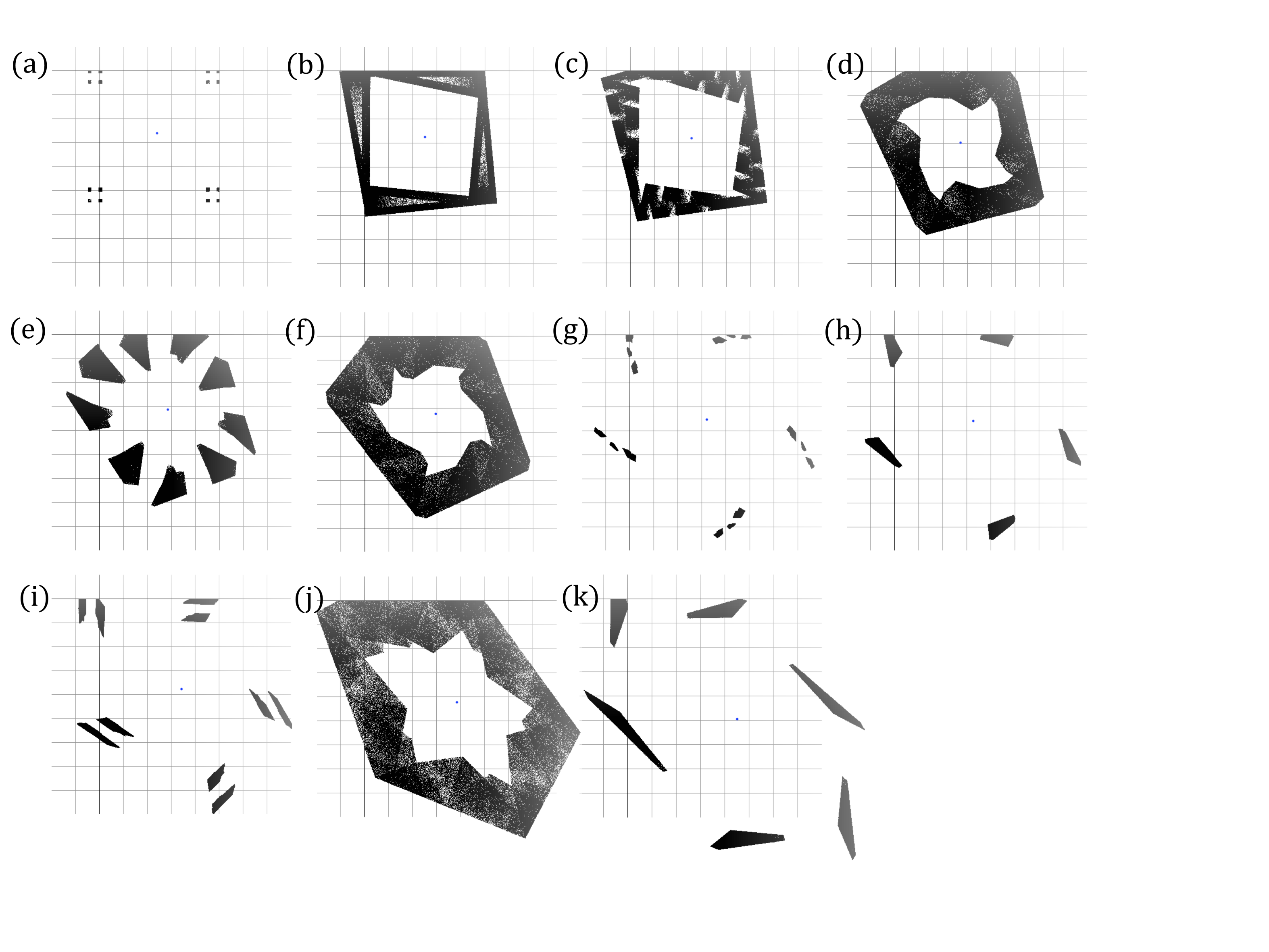
Figure 1: Numerical illustration of asymptotic periodicity in (29). We show the support of $\{P^{500}f_{0}\}$ for an initial density $f_{0}=1_{[-5,5]\times[-5,5]}$, approximated by $1,000\times 1,000$ initial points uniformly distributed on $[-5,5]\times[-5,5]$ and various values of $\alpha$ with $\beta=1.1$. (a) $\alpha=0.0$, Period $=16$; (b) $\alpha=0.1$, Period $=1$; (c) $\alpha=0.14$, Period $=1$; (d) $\alpha=0.25$, Period $=1$; (e) $\alpha=0.34$, Period $=9$; (f) $\alpha=0.4$, Period $=1$; (g) $\alpha=0.54$, Period $=12$; (h) $\alpha=0.57$, Period $=5$; (i) $\alpha=0.64$, Period $=10$; (j) $\alpha=0.8$, Period $=1$; (k) $\alpha=0.99$, Period $=6$.

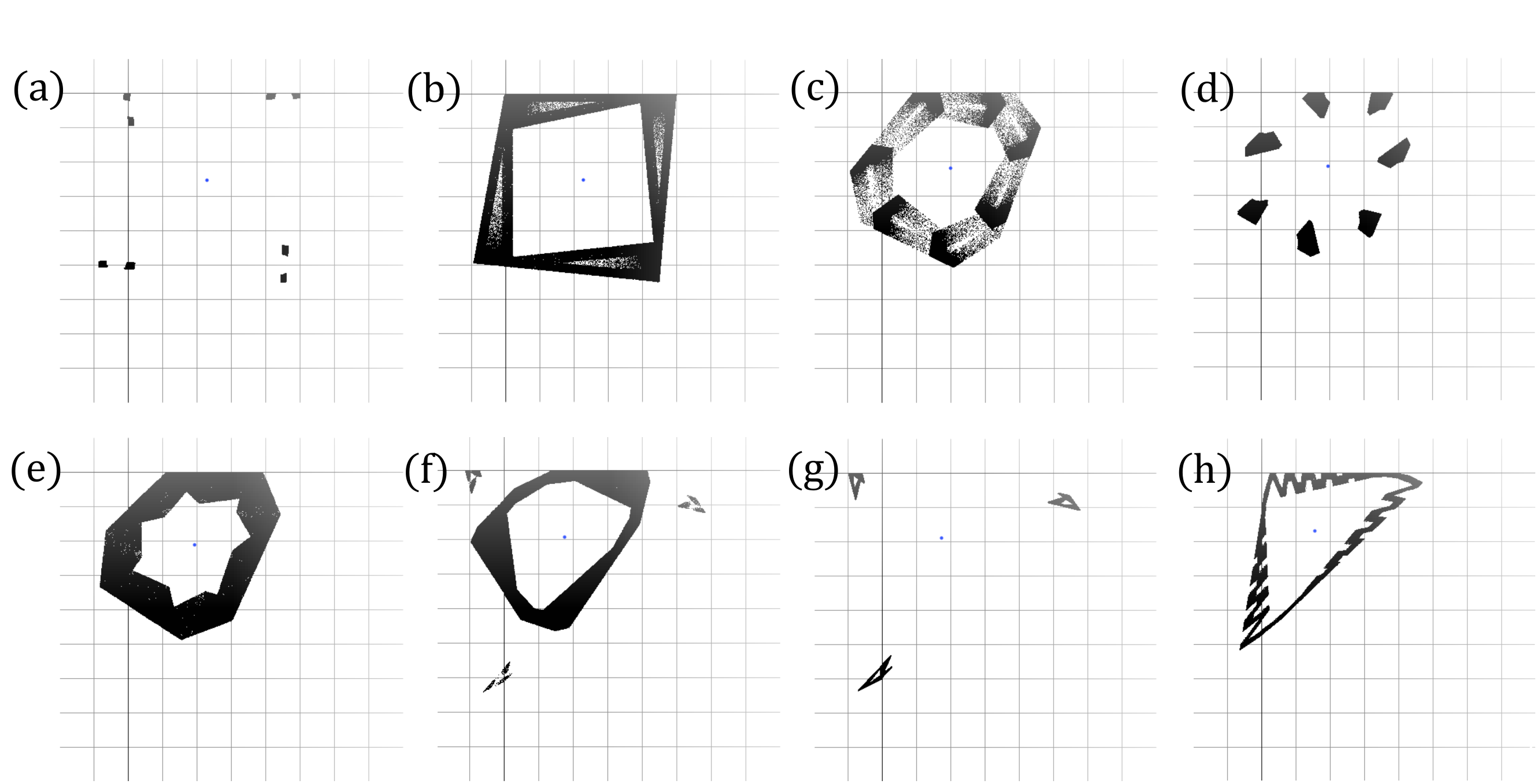
Figure 2: As in Figure 1 with $\beta=1.1$. (a) $\alpha=-0.08$, Period $=8$; (b) $\alpha=-0.1$, Period $=1$; (c) $\alpha=-0.41$, Period $=1$; (d) $\alpha=-0.46$, Period $=7$; (e) $\alpha=-0.5$, Period $=1$; (f) $\alpha=-0.75$, Period $=3$; (g) $\alpha=-0.8$, Period $=3$; (h) $\alpha=-1.14$, Period $=1$;.

For smaller $\beta=1.02$ in Figure 3 we observe higher periods (Period: (a) 13, (c) 35, (e) 22, (g) 31). In addition to this, we find period $9$ when $\alpha=0.35$. These numerical values of the periods may be related to a Farey series, see Section 4.3.

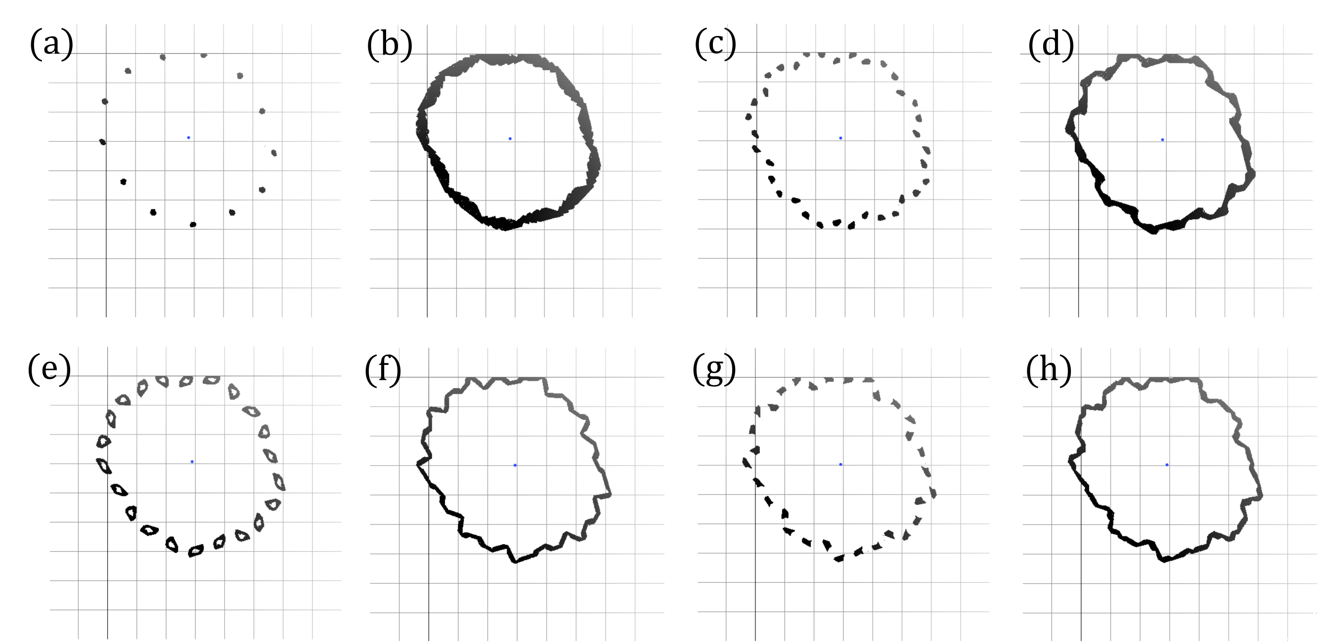
Figure 3: As in Figure 1 with $\beta=1.02$. (a) $\alpha=0.24$, Period $=13$; (b) $\alpha=0.25$, Period $=1$; (c) $\alpha=0.27$, Period $=35$; (d) $\alpha=0.28$, Period $=1$; (e) $\alpha=0.284$, Period $=22$; (f) $\alpha=0.3$, Period $=1$; (g) $\alpha=0.3015$, Period $=31$; (h) $\alpha=0.31$, Period $=1$;.

4.2 Discussion: Asymptotic periodicity

Consider (29) in the context of Corollary 3.3. Since (29) is piecewise linear and the Jacobian $\lambda_{n}$ for $\tilde{S}^{n}$ is $\beta^{n}$, the assumptions (i)-(iv) of Theorem 3.1 are satisfied. Thus we need only show the condition (v) holds, that is, $\frac{5}{2\beta^{N}}r_{n}<1$ where $r_{n}$ denotes the number of partitions for $\tilde{S}^{n}$.

Without loss of generality, it is enough to consider the system (29) on the half plane $\mathbb{R}_{\{y\leq 0\}}$ since all points are in $\mathbb{R}_{\{y\leq 0\}}$ after iterating once. Let $L$, $M$ and $R$ be the sets $L=\{(x,y)\in\mathbb{R}^{2}\ |\ x<0,y<0\}$, $M=\{(x,y)\in\mathbb{R}^{2}\ |\ x=0,y<0\}$ and $R=\{(x,y)\in\mathbb{R}^{2}\ |\ x>0,y<0\}$ respectively, and denote

$$S_{L}(x,y)=(\alpha x+y+1,\beta x)\ \ (x<0),\ \ \ \ S_{R}(x,y)=(\alpha x+y+1,-\beta x)\ \ (x\geq 0).$$ (32)

One immediately has the following properties for (29):

• If $\alpha+\beta>1$, there exists a fixed point $(x_{L}^{\ast},y_{L}^{\ast})=(\frac{1}{1-\alpha-\beta},\frac{\beta}{1-\alpha-\beta})\in L$.

• If $\alpha-\beta<1$, there exists a fixed point $(x_{R}^{\ast},y_{R}^{\ast})=(\frac{1}{1-\alpha+\beta},\frac{-\beta}{1-\alpha+\beta})\in R$.

• The eigenvalues of the Jacobian are $\lambda_{L}^{\pm}=\frac{\alpha\pm\sqrt{\alpha^{2}+4\beta}}{2}$ and $\lambda_{R}^{\pm}=\frac{\alpha\pm\sqrt{\alpha^{2}-4\beta}}{2}$, and the corresponding eigenvectors are $(\lambda_{L}^{\pm},\beta)$ and $(\lambda_{R}^{\pm},-\beta)$.

• Since $\alpha^{2}+4\beta>0$ always holds, $\lambda_{L}^{+}>1$ if $\alpha+\beta>1$. This implies the fixed point $x_{L}^{\star}$ is unstable.

• If $\alpha^{2}\geq 4\beta$ and $\alpha>2$, then $\lambda_{R}^{+}>1$ and $x_{R}^{\ast}$ is an unstable node, and almost all points diverge in this case.

• In the case $\alpha^{2}<4\beta$, then $\lambda_{R}^{\pm}$ is complex which implies $x_{R}^{\ast}$ is an unstable focus (if $\alpha>0$), a center (if $\alpha=0$) and a stable focus (if $\alpha<0$).

Based on these observations, we focus on parameters satisfying $\alpha+\beta>1$, $\alpha-\beta<1$, $\alpha^{2}<4\beta$, $\alpha>0$ and $1<\beta\leq 2$. Note that although asymptotic periodicity is observed even when $\alpha<0$ (Figure 2), here we assume $\alpha>0$ to simplify the arguments.

First, we know the saddle point $x_{L}^{\star}\in L$. Let $D_{0}$ be the set

$$D_{0}:=\{(x,y)\in L\cup M\ |\ y-y_{L}^{\ast}<\frac{\beta}{\lambda_{L}^{-}}(x-x_{L}^{\ast})\}.$$ (33)

From the instability of the fixed point $(x_{L}^{\ast},y_{L}^{\ast})$, one can immediately conclude that all points in $D_{0}$ eventually diverge. Next, let $c$ be a $y$-intercept of the line $y-y_{L}^{\ast}<\frac{\beta}{\lambda_{L}^{-}}(x-x_{L}^{\ast})$, that is, $c=\beta x_{L}^{\ast}(1-1/\lambda_{L}^{-})$. Then the $x$-intercept of the line can be calculated as $S_{L}(0,c)=c+1$ which is always negative when $\alpha+\beta>1$.

Second, consider the inverse sets $D_{i}:=S_{R}^{-i}(D_{0})\cap\mathbb{R}_{\{y\leq 0\}}$ and the inverse of a point $(0,c)$, $S_{R}^{-i}(0,c)$ for $i=1,2,3,\cdots$. Note that all points in $D_{i}$ for some $i$ diverge. Now let $\ell$ be a minimum number $i$ such that the $y$-coordinate of $S_{R}^{-i}(0,c)$ is positive. Then let $C$ be a set defined by

$$C:=\mathbb{R}_{\{y\leq 0\}}\backslash\bigcup_{i=0}^{\ell}{D_{i}}.$$ (34)

Then $C$ becomes the candidate for the attracting region. Figure 4 illustrates the partition of the half plane ($y\leq 0$) and regions $C$ and $\{D_{i}\}_{i=0}^{\ell}$ for the case $\ell=5$.

Third, let $p$ (and $q$) be the $x$-coordinate of the intersection point of the line $y=0$ and the line generated by $S_{R}^{-\ell}(0,c)$ and $S_{R}^{-(\ell-1)}(0,c)$ (and $S_{R}^{-\ell}(0,c)$ and $(x_{R}^{*},y_{R}^{*})$). We can consider three cases depending on the values of $p,q$ relative to $1$.

Figure 5 illustrates the three possible cases. Figure 5 (a) shows the case in which both $p,q<1$, (b) shows the case $p<1<q$, and (c) shows the case with $1<p,q$. We immediately observe that points in $C$ may leave from $C$ in case (a) because of the black region, and if $q\geq 1,$ then $C$ is a conserved region. Therefore, we can construct a dynamical system which acts on a bounded set by giving the restricted system $\tilde{S}:C\to C$ for the case (b) or (c). We focus on case (b).

From these observations, there exists a partition $I_{0},\cdots,I_{\ell+1}$ in $C$ such that $\tilde{S}^{\ell+2}(I_{i})\subset I_{i}$ for any $i=0,\cdots,\ell+1$ (see Figure 6). The condition (iv) implies the ratio of entry point of the before and after curve by the inverse transformation. In our case, an increase of the number of entry points happens only for the $S|_{I_{\ell+1}}^{-1}$, in other words, the other $S|_{I_{i}}^{-1}$, $i=0,\cdots,\ell$ does not increase the entry points because of the rotational behavior. Since $\beta>1$, for some $t$, $\beta^{t}$ which is the Jacobian of $\tilde{S}^{t}$, might be larger than $C$. Namely, the condition (iv) and (v) in Theorem 3.1 would be satisfied for $\tilde{S}^{t}$ with sufficiently large $t$.

However, it is difficult to check the condition (iv) because of the impossibility to calculate the change of entry points for all curves. Thus, we do not have checkable sufficient conditions for the assumption (iv) to prove asymptotic periodicity for $\tilde{S}$, which is strongly suggested by the numerical results. In the case (c), although it is more complicated due to the black region, we may use similar arguments after one more iterate $S^{-(\ell+1)}_{R}(0,c)$.

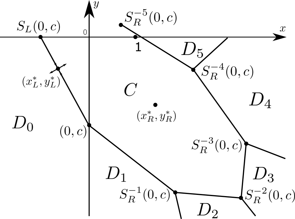
Figure 4: The regions $D_{i}$, $i=0,1,\cdots,5$, and $C$ are illustrated when $\ell=5$. The fixed point $(x_{L}^{*},y_{L}^{*})$ is a saddle and $(x_{R}^{*},y_{R}^{*})$ is an unstable focus,

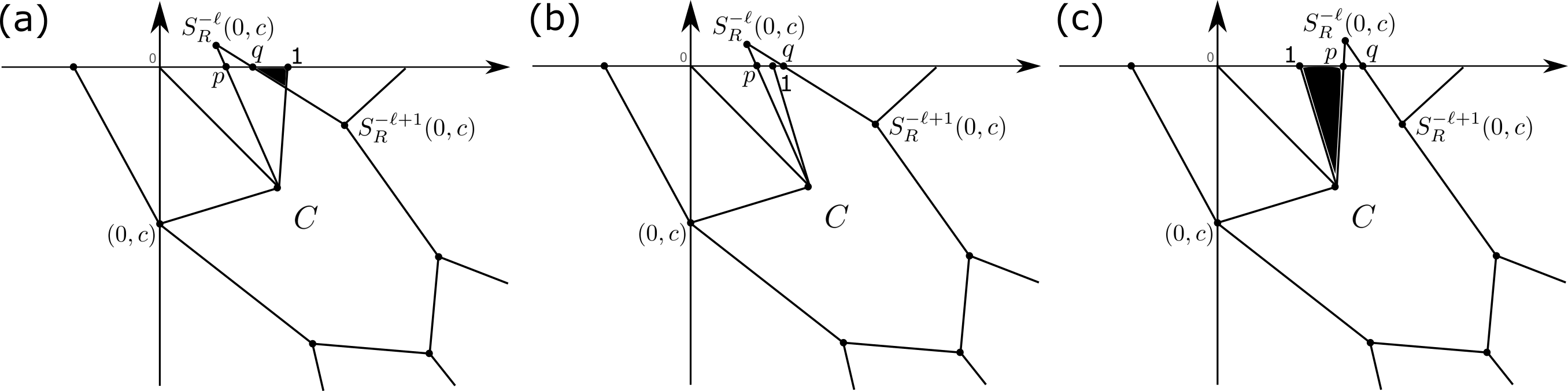
Figure 5: The situation can be separated into three cases depending on positions of $p,q$ and $1$. (a) the case $p,1<1$, (b) the case $p<1<q$, and (c) the case $1<p,q$.

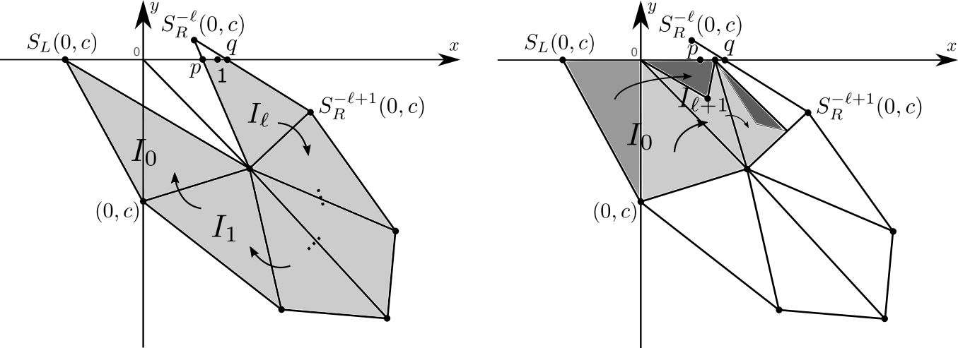
Figure 6: Illustrations of the result of iterating the regions $\{I_{i}\}_{i=0}^{\ell+1}$ by $\tilde{S}$.

Finally, we will estimate the parameter conditions such that $q\geq 1$ since at least $q$ must be larger than 1 to be a conservative system. If we set $S_{R}^{-1}({\bm{x}})=A{\bm{x}}+{\bm{b}}$, then $S_{R}^{-n}({\bm{x}})=A^{n}{\bm{x}}+(A^{n-1}+\cdots+A+I){\bm{b}}$ where

$$A=\begin{pmatrix}0&-1/\beta\\ 1&\alpha/\beta\end{pmatrix},\ \ \ \bm{b}=\begin{pmatrix}0\\ -1\end{pmatrix}.$$

Thus we have

$$A^{n}=\frac{1}{\nu_{-}-\nu_{+}}\begin{pmatrix}\nu_{+}^{n}\nu_{-}-\nu_{+}\nu_{-}^{n}&(-\nu_{+}^{n}+\nu_{-}^{n})/\beta\\ (\nu_{+}^{n+1}\nu_{-}-\nu_{+}\nu_{-}^{n+1})\beta&-\nu_{+}^{n+1}+\nu_{-}^{n+1}\end{pmatrix},$$

where $\nu_{\pm}$ are eigenvalues of $A$ with $\nu_{\pm}=\frac{\alpha}{2\beta}\pm\frac{\sqrt{4\beta-\alpha^{2}}}{2\beta}i\in\mathbb{C}$. By using the above equations, we may write $S^{-n}(0,c)$, $p$ and $q$ explicitly. However, not only is the calculation complicated, but also we cannot obtain the number $\ell$ for each set of parameters. Thus we numerically show only approximate values of $\alpha$ which gives the condition for $q\geq 1$ for some values of $\beta$ in Table 1.

$\beta$	$\ell$	$\alpha<$	$\beta$	$\ell$	$\alpha<$	$\beta$	$\ell$	$\alpha<$	$\beta$	$\ell$	$\alpha<$
1.01	14	1.85664	1.06	7	1.57519	1.2	4	1.15624	1.7	3	0.53436
1.02	11	1.78516	1.07	7	1.56379	1.3	3	1.03992	1.8	2	0.32593
1.03	9	1.71214	1.08	6	1.48766	1.4	3	0.78308	1.9	2	0.13439
1.04	8	1.65753	1.09	6	1.46841	1.5	3	0.66496	2.0	2	0.00000
1.05	8	1.64245	1.1	5	1.45765	1.6	3	0.58999

Table 1: For each $\beta$, the value $\alpha$ which gives the condition for $q\geq 1$ are calculated numerically.

4.3 Discussion: Period

We would like to be able to predict the period of the asymptotic periodicity in (29) for a given set of parameters $(\alpha,\beta)$, but although we can make a partition $\{I_{i}\}_{i=0}^{\ell+1}$ as the previous section, we cannot find the period or the relation between $\ell$ and period.

The numerical results in Figure 1,2 and 3 tantalizingly remind one of the Farey series. In dynamical systems, periodic structures based on the Farey series sometimes appear, for instance in circle map models of cardiac arrhythmias [36, 38, 37]. The fraction $l/n$ corresponds to a rotation number of the system, that is, every periodic orbit has period $n$. Nakamura [11] proved that the Markov operator corresponding to the perturbed piecewise linear map (2) exhibits asymptotically periodicity, and clarified the relationship of the periods associated with the Farey series for various parameters.

For our example (29), Figure 3 displays asymptotic periodicity with period 22 in between values of the parameter $\alpha$ giving rise to period 13 and 9, while period 35 is between 13 and 22, and period 31 is between 22 and 9. Moreover, we observe period $58$ $(\alpha=0.322)$, $76$ $(\alpha=0.328)$ and $47$ $(\alpha=0.42)$. That is, there exist parameters for which the system has asymptotic periodicity with period $p_{1}+p_{2}$ between the parameters which give periods $p_{1}$ and $p_{2}$. To take this observation and relate the periodicity of (29) to the Farey series is a matter for future research.

References

- [1] L. Boltzmann, Lectures on gas theory, Courier Corporation, 2012.
- [2] J.W. Gibbs Elementary Principles in Statistical Mechanics, Dover, New York, 1962.
- [3] A. Lasota, and M.C. Mackey, Chaos, fractals, and noise: stochastic aspects of dynamics. Springer Science & Business Media, New York, 2013.
- [4] F. Hofbauer and G. Keller, Ergodic properties of invariant measures for piecewise monotonic transformations, Math. Z, 180 (1982), 120–141.
- [5] A. Lasota, T.Y. Li and J.A. Yorke, Asymptotic periodicity of the iterates of Markov operators Transactions of the American Mathematical Society, 286(2) (1984), 751–764.
- [6] J. Komorník, Asymptotic periodicity of the iterates of weakly constrictive Markoy operators, Tohoku Mathematical Journal, Second Series, 38(1) (1986), 15–27.
- [7] A. Lasota and J.A. Yorke, Statistical periodicity of deterministic systems, Časopis pro pěstování matematiky, 111(1) (1986), 1–13.
- [8] N. Provatas and M.C. Mackey, Asymptotic periodicity and banded chaos, Physica D. Nonlinear Phenomena, 53(2–4) (1991), 295–318.
- [9] A. Lasota and M.C. Mackey, Noise and statistical periodicity, Physica D. Nonlinear Phenomena, 28(1–2) (1987), 143–154.
- [10] N. Provatas and M.C. Mackey, Noise-induced asymptotic periodicity in a piecewise linear map, Journal of statistical physics, 63(3–4) (1991), 585–612.
- [11] F. Nakamura, Asymptotic behavior of non-expanding piecewise linear maps in the presence of random noise, Discrete & Continuous Dynamical Systems-B, 23(6) (2018), 2457–2473.
- [12] S. Ito, S. Tanaka and H. Nakada, On unimodal linear transformations and chaos. I, Tokyo Journal of Mathematics 2 (1979) 221–239.
- [13] S. Ito, S. Tanaka and H. Nakada, On unimodal linear transformations and chaos. II Tokyo Journal of Mathematics 2 2 (1979), 241–259.
- [14] H. Shigematsu, H. Mori, T. Yoshida and H. Okamoto, Analytic study of power spectra of the tent maps near band-splitting transitions, Journal of Statistical Physics 30(3) (1983), 649–679.
- [15] T. Yoshida, H. Mori and H. Shigematsu, Analytic study of chaos of the tent map: band structures, power spectra, and critical behaviors, Journal of Statistical Physics, 31(2) (1983) 279–308.
- [16] J. Nagumo and S. Sato, On a response characteristic of a mathematical neuron model, Kybernetik, 10(3) (1972), 155–164.
- [17] J.P. Keener, Chaotic behavior in piecewise continuous difference equations, Transactions of the American Mathematical Society, 261(2) (1980), 589–604.
- [18] P. Gora and A. Boyarsky, Absolutely continuous invariant measures for piecewise expanding transformations in , Israel journal of Mathematics, 67(3) (1989), 272–286.
- [19] M. C. Mackey. Time’s Arrow: The Origins of Thermodynamic Behaviour, Springer-Verlag, Berlin, New York, Heidelberg, 1992.
- [20] J. Komorník and A. Lasota, Asymptotic decomposition of Markov operators, emphBulletin of the Polish Academy of Sciences. Mathematics, 35(5–6) (1987), 321–327.
- [21] J. Komorník, Asymptotic periodicity of Markov and related operators, Dynamics reported, 2 (1993), 31–68.
- [22] G. Vitali, Sulle funzione integrali, Atti Accad. Sci. Torino Cl. Sci. Fis. Mat. Natur., 40 (1904/1905), 1021–1034.
- [23] G.H. Hardy, On double Fourier series, and especially those which represent the double zeta-function with real and incommensurable parameters, Quart. J. Math. Oxford, 37 (1905/1906), 53–79.
- [24] C.R. Adams and J.A. Clarkson, Properties of functions of bounded variation, Transactions of the American Mathematical Society, 36(4) (1934), 711–730.
- [25] V.V. Chistyakov and Y.V. Tretyachenko, Maps of several variables of finite total variation. I. Mixed differences and the total variation, Journal of Mathematical Analysis and Applications, 370(2) (2010), 672–686.
- [26] B. Ashton and I. Doust, Functions of bounded variation on compact subsets of the plane, Studia Mathematica, 169 (2005), 163–188.
- [27] J. Giménez, N. Merentes and M. Vivas, Functions of bounded variation on compact subsets of C, Commentationes Mathematicae, 54(1) (2014), 3–19.
- [28] H. Toyokawa, -finite invariant densities for eventually conservative Markov operators, Discrete & Continuous Dynamical Systems-A, 40(5) (2020), 2641–2669.
- [29] I. Sushko and L. Gardini, Center bifurcation for two-dimensional border collision normal form, International Journal of Bifurcation and Chaos, 18(4) (2008), 1029–1050.
- [30] R. Lozi, Un attracteur étrange (?) du type attracteur de Hénon, Le Journal de Physique Colloques, 39 C5 (1978), C5–9.
- [31] H. E. Nusse and J. A. Yorke, Border-collision bifurcations including “period two to period three” for piecewise smooth systems, Physica D: Nonlinear Phenomena, 57(1-2), (1992), 39–57.
- [32] M. Hénon, A two-dimensional mapping with a strange attractor, The Theory of Chaotic Attractors, (1976), 94–102.
- [33] Z. Elhadj and J.C. Sprott, A new simple 2-D piecewise linear map, Journal of Systems Science and Complexity, 23(2) (2010), 379–389.
- [34] J. Losson and M.C. Mackey, Coupled map lattices as models of deterministic and stochastic differential delay equations, Physical Review E. Statistical, Nonlinear, and Soft Matter Physics, 52 1 part A (1995) 115–128.
- [35] T. M. Apostol, Modular Functions and Dirichlet Series in Number Theory, Springer-Verlag, New York-Heidelberg, 1976.
- [36] P.L. Boyland, Bifurcations of circle maps: Arnol’d tongues, bistability and rotation intervals, Communications in Mathematical Physics, 106(3) (1986), 353–381.
- [37] G. Swiatek, Rational rotation numbers for maps of the circle, Communications in mathematical physics, 119 (1988), 109–128.
- [38] L. Glass, M.R. Guevara, A. Shrier and R. Perez, Bifurcation and chaos in a periodically stimulated cardiac oscillator, Physica D: Nonlinear Phenomena, 7(1–3), (1983), 89–101.