Linearly Implicit Multistep Methods for Time Integration

Abstract

Time integration methods for solving initial value problems are an important component of many scientific and engineering simulations. Implicit time integrators are desirable for their stability properties, significantly relaxing restrictions on timestep size. However, implicit methods require solutions to one or more systems of nonlinear equations at each timestep, which for large simulations can be prohibitively expensive. This paper introduces a new family of linearly implicit multistep methods (Limm), which only requires the solution of one linear system per timestep. Order conditions and stability theory for these methods are presented, as well as design and implementation considerations. Practical methods of order up to five are developed that have similar error coefficients, but improved stability regions, when compared to the widely used BDF methods. Numerical testing of a self-starting variable stepsize and variable order implementation of the new Limm methods shows measurable performance improvement over a similar BDF implementation.

65L04, 65L05, 65L06

1 Introduction

In this paper we are concerned with the numerical solution of initial value problems (IVP):

(1) $$\frac{dy}{dt}=f(t,y),\quad t_{0}\leq t\leq t_{F},\quad y(t_{0})=y_{0};\quad y(t)\in\mathbb{R}^{N},~{}~{}f:\mathbb{R}\times\mathbb{R}^{N}\rightarrow\mathbb{R}^{N}.$$

Systems of ordinary differential equations (ODEs) of this form appear in a wide variety of scientific and engineering simulations. Some types of simulations, such as those of chemical kinetics or aerosol dynamics [14, 36], can be directly modeled by systems of densely coupled ODEs. Others, such as those of fluid dynamics [24], arise from the semi-discretization in space of partial differential equations (PDEs) via the method of lines, resulting in a large sparse system of ODEs.

Two time integration families of methods are used to discretize (1): explicit or implicit. Explicit schemes advance the solution to a new timestep using only information from previous steps, and are simple in structure with very low computational cost per timestep. However, they have stability limitations that result in problem-dependent bounds on the largest allowable stepsizes. For stiff problems, implicit time integration methods that determine solutions at a new timestep using both past and future information, are preferable. These schemes avoid stability-bound stepsize limitations at the cost of solving one or more nonlinear systems per timestep.

As solving large nonlinear systems can be very expensive, many types of linearly implicit methods have been developed that only require solutions of linear systems at each step. Rosenbrock methods [32] (and their many extensions [40, 29, 28, 37, 45, 43, 16]) are linearized implicit Runge-Kutta methods. Implicit-explicit (IMEX) methods [12, 48, 49, 1, 2] couple an implicit scheme for the stiff component with an explicit scheme for the non-stiff component of a split problem. A common splitting treats the nonlinear part of the problem explicitly and the linear part implicitly, therefore avoiding the need for nonlinear solves. Exponential integrators [22, 41, 42, 25, 26] also effectively treat a linear-nonlinear problem splitting, with the linear portion solved via an exponential integrating factor. It is also common to linearize implicit methods which would normally require nonlinear solves by taking only a single Newton iteration [46, 39], or to replace parts of the implicit scheme with an extrapolation of past values [15, 47, 10, 11], at the possible cost of order reduction and/or reduced stability.

In this paper we construct linearly implicit multistep methods (Limm) in much the same way that Rosenbrock methods are obtained from implicit Runge-Kutta methods. We determine order conditions which account for the linearization [5, 20], and solve for a family of $k$-step order $k$ methods for $k=1,\dots,5$. Limm methods have more free coefficients than traditional linear multistep methods with the same number of steps, and this additional freedom enables the optimization of accuracy and stability properties. The new schemes designed herein have linear stability regions larger than, and error constants comparable to, the widely used BDF [13] family of methods.

The remainder of the paper is organized as follows. Section 2 describes the construction of the Limm general form. Section 3 builds order conditions for $k$-step Limm methods of order $p$. Section 4 considers the linear stability of Limm methods, and Section 5 their convergence for step sizes not limited by the stiffness of the system. Section 7 discusses the design of new methods with optimal stability properties and error coefficients, and develops a family of $k$-step order $k$ methods with $k=1,\dots,5$. Section 8 provides the details necessary for an efficient implementation of Limm methods with variable stepsize and variable order. Section 9 reports numerical results comparing Limm to BDF methods. Finally, Section 10 draws concluding remarks.

2 Linearly Implicit Multistep Methods

A linear $k$-step method computes the solution of (1) as follows [20, Chapter III.2]:

(2) $$\sum_{i=-1}^{k-1}\alpha_{i}\,y_{n-i}=h_{n}\sum_{i=-1}^{k-1}\beta_{i}\,f(t_{n-i},y_{n-i}),$$

where the numerical solution $y_{n-i}\approx y(t_{n-i})$ and the step size is $h_{n}=t_{n+1}-t_{n}$. The simplest way to obtain a linearly implicit multistep method is to linearize the implicit evaluation of $f(t_{n+1},y_{n+1})$ in (2) about $\left(t_{n},y_{n}\right)$, to obtain:

(3) $$\begin{split}\sum_{i=-1}^{k-1}\alpha_{i}\,y_{n-i}&=h_{n}\,\sum_{i=0}^{k-1}\,\beta_{i}^{\prime}\,f(t_{n-i},y_{n-i})\\ &+h_{n}\beta_{-1}\,f_{y}(t_{n},y_{n})\,(y_{n+1}-y_{n})+h_{n}^{2}\beta_{-1}\frac{\partial f}{\partial t}(t_{n},y_{n}),\end{split}$$

where $\beta_{0}^{\prime}=\beta_{0}+\beta_{-1}$, $\beta_{i}^{\prime}=\beta_{i}$ for $i=1,\dots,k-1$.

Remark 2.1 (Autonomous and non-autonomous forms).

In order to simplify the notation in the remainder of the paper, we will make use of the autonomous form of (1), with $\frac{dy}{dt}=f(y)$ and the notation

$$f_{n}\coloneqq f(y_{n}),\quad\mathbf{J}_{n}\coloneqq f_{y}(y_{n}).$$

As the original non-autonomous form can be recovered by stacking $t$ with the vector $y$ and making corresponding changes to $f$ and $\mathbf{J}$, the methods developed for autonomous problems are also applicable to non-autonomous problems.

Now, because the direct linearization approach in (3) maintains the same number of degrees of freedom, one can expect a degradation of accuracy and stability properties of (3) when compared to the standard nonlinear scheme (2) with the same number of steps. In order to increase the number of degrees of freedom one can generalize the approach by retaining in the formulation past linearized steps scaled by new $\mu$ coefficients:

(4) $$\sum_{i=-1}^{k-1}\alpha_{i}\,y_{n-i}=h_{n}\,\sum_{i=0}^{k-1}\beta_{i}\,f_{n-i}+h_{n}\,\sum_{i=-1}^{k-1}\mu_{i}\,\mathbf{J}_{n-i-1}\,y_{n-i}.$$

However, method (4) requires the storage of multiple past Jacobian-vector products in addition to past solutions and function values, which is not desirable. For this reason we consider a hybrid of the two approaches (3) and (4), and, drawing inspiration from Rosenbrock methods [32], [21, Section IV.7], define the following computational process.

Definition 2.2 (Limm methods).

A linearly implicit multistep method (Limm) advances the numerical solution of (1) over one step $[t_{n},t_{n+1}]$ as follows:

(5) $$\sum_{i=-1}^{k-1}\alpha_{i}\,y_{n-i}=h\,\sum_{i=0}^{k-1}\beta_{i}\,f_{n-i}+h_{n}\,\mathbf{J}_{n}\,\left(\sum_{i=-1}^{k-1}\mu_{i}\,y_{n-i}+h_{n}\,\sum_{i=0}^{k-1}\nu_{i}\,f_{n-i}\right),$$

where, without loss of generality, $\alpha_{-1}=1$.

A linearly implicit multistep method of W-type (Limm-w) advances the numerical solution using (5), where the exact Jacobian $\mathbf{J}_{n}$ is replaced by an arbitrary matrix $\mathbf{A}_{n}$. This matrix is chosen to ensure the numerical stability of the scheme, but without impacting the order of accuracy of the method.

The non-autonomous form of (5) adds the following term to the right side of equation (5)

$$h_{n}\,\frac{\partial f}{\partial t}(t_{n},y_{n})\,\left(\sum_{i=-1}^{k-1}\mu_{i}t_{n-i}+h_{n}\sum_{i=0}^{k-1}\nu_{i}\right).$$

We note that $k$-step Limm schemes (5) have $4k+1$ free coefficients (compared to $2k+1$ for classical nonlinear methods (2)), and require storing only $k$ past solution and $k$ past function values at each step (the same as nonlinear methods (2)). Evaluation of the Limm numerical solution at each step (5) requires to only solve a linear system of equations, expressed in a computationally efficient form as:

$$\begin{split}\left(\mathbf{I}-h_{n}\,\mu_{-1}\,\mathbf{J}_{n}\right)\cdot z&=\sum_{i=0}^{k-1}\left(\mu_{i}/\mu_{-1}-\alpha_{i}\right)\,y_{n-i}+h_{n}\,\sum_{i=0}^{k-1}\left(\nu_{i}/\mu_{-1}+\beta_{i}\right)\,f_{n-i},\\ y_{n+1}&=z-\sum_{i=0}^{k-1}(\mu_{i}/\mu_{-1})\,y_{n-i}-h_{n}\,\sum_{i=0}^{k-1}(\nu_{i}/\mu_{-1})\,f_{n-i}.\end{split}$$

Rosenbrock-W methods [21, Section IV.7] seek to increase the computational efficiency of Rosenbrock methods by replacing the exact Jacobian $\mathbf{J}_{n}$ with an arbitrary matrix $\mathbf{A}_{n}$, such that the corresponding linear system at each step can be solved more easily. This concept is extended to linearly implicit multistep methods by considering Limm-w schemes.

3 Order Conditions

Derivation of the order conditions amounts to equating the Taylor series coefficients of the numerical and exact solutions about the current time $t_{n}$, up to a specific predetermined order. This is the approach taken for building the classical order condition theory for linear multistep methods [20, Chapter III.2]. We discuss a direct Taylor series approach to obtain order conditions for Limm-w schemes in Section 3.1. However, constructing Taylor series by repeatedly differentiating the numerical solution becomes increasingly difficult for high-order schemes, and we use a B-series approach [20, 5] to derive Limm order conditions in Section 3.2.

We assume that the linearly implicit scheme (5) computes the solution at a non-uniform time grid $t_{n-i}$, and express the distances between the solution points as fractions of the current step $h_{n}=t_{n+1}-t_{n}$:

(6a) $$t_{n-i}=t_{n}-c_{i}\,h_{n},\quad i=-1,\dots,k;\qquad c_{-1}=-1,\quad c_{0}=0.$$

Many adaptive step analyses consider the ratios of consecutive step sizes $$\omega_{n} c_{i}$$. One can express as a function of these step size ratios as follows:

(6b) $$\begin{split}&t_{n-\ell+1}-t_{n-\ell}=(t_{n+1}-t_{n})\prod_{j=0}^{\ell+1}\frac{t_{n-j}-t_{n-j-1}}{t_{n-j+1}-t_{n-j}}=h\,\prod_{j=0}^{\ell+1}\omega_{n-j}^{-1},\\ &t_{n}=t_{n-i}+\sum_{\ell=1}^{i}(t_{n-\ell+1}-t_{n-\ell})=t_{n-k}+h\,\sum_{\ell=1}^{i}\prod_{j=0}^{\ell+1}\omega_{n-j}^{-1},\\ &\omega_{n}=\frac{t_{n+1}-t_{n}}{t_{n}-t_{n-1}},\qquad c_{i}=\sum_{\ell=1}^{i}\prod_{j=0}^{\ell+1}\omega_{n-j}^{-1},\qquad i\geq 1.\end{split}$$

Remark 3.1 (Method coefficients notation).

When operating on this non-uniform time grid, all the coefficients, $\alpha_{i}$, $\beta_{i}$, $\mu_{i}$, and $\nu_{i}$, $i\in[-1,k-1]$, of method (5) are, in general, functions of the stepsize fractions $c_{j}$, $j\in[1,k]$ (or analogously, of the stepsize ratios $\omega_{n}$). In order to simplify our notation, we will leave out the function notation unless it is needed for clarity, and will explicitly call out when we are only considering fixed-stepsize methods (as in the latter half of Section 7).

3.1 Order conditions for Limm-w methods

The order conditions for Limm-w methods (5) can be obtained by the standard Taylor series approach, leading to the following result.

Theorem 3.2 (Limm-w order conditions).

The Limm-w method (5) has order of consistency $p$ if and only if its coefficients satisfy:

(7a) $$\sum_{i=-1}^{k-1}\alpha_{i} =0,$$

(7b) $$\sum_{i=-1}^{k-1}\mu_{i} =0,$$

(7c) $$\sum_{i=-1}^{k-1}\alpha_{i}\,c_{i}^{\ell}+\ell\,\sum_{i=0}^{k-1}\beta_{i}\,c_{i}^{\ell-1} =0,\qquad\ell=1,\dots,p,$$

(7d) $$\sum_{i=-1}^{k-1}\mu_{i}\,c_{i}^{\ell-1}-(\ell-1)\,\sum_{i=0}^{k-1}\nu_{i}\,c_{i}^{\ell-2} =0,\qquad\ell=2,\dots,p.$$

Proof 3.3.

We show that the local truncation error is of order $p+1$. To this end we apply the method (5) starting with exact past solution values:

(8) $$\begin{split}y_{n+1}+\sum_{i=0}^{k-1}\alpha_{i}\,y(t_{n-i})&=h_{n}\,\sum_{i=0}^{k-1}\beta_{i}\,y^{\prime}(t_{n-i})+h_{n}\,\mathbf{A}_{n}\,\sum_{i=0}^{k-1}\mu_{i}\,y(t_{n-i})\\ &\quad+h_{n}\,\mu_{-1}\,\mathbf{A}_{n}\,y_{n+1}+h_{n}\,\mathbf{A}_{n}\,\sum_{i=0}^{k-1}\nu_{i}\,h_{n}\,f(t_{n-i},y(t_{n-i})),\end{split}$$

and show that $y_{n+1}-y(t_{n+1})\sim\mathcal{O}(h_{n}^{p+1})$. We insert the exact solution in (8):

(9) $$\begin{split}\sum_{i=-1}^{k-1}\alpha_{i}\,y(t_{n-i})&=h_{n}\,\sum_{i=0}^{k-1}\beta_{i}\,y^{\prime}(t_{n-i})+h_{n}\,\mathbf{A}_{n}\,\sum_{i=-1}^{k-1}\mu_{i}\,y(t_{n-i})\\ &\quad+h_{n}^{2}\,\mathbf{A}_{n}\,\sum_{i=0}^{k-1}\nu_{i}\,y^{\prime}(t_{n-i})+r_{n},\end{split}$$

where $r_{n}$ is the local residual, and expand in Taylor series about the current time $t_{n}$

$$\begin{split}&\sum_{\ell\geq 0}\sum_{i=-1}^{k-1}\alpha_{i}\,\frac{(-c_{i})^{\ell}\,h_{n}^{\ell}}{\ell!}y^{(\ell)}(t_{n})=\sum_{\ell\geq 1}\sum_{i=0}^{k-1}\beta_{i}\,\frac{(-c_{i})^{\ell-1}\,h_{n}^{\ell}}{(\ell-1)!}y^{(\ell)}(t_{n})\\ &+\mathbf{A}_{n}\,\sum_{\ell\geq 1}\sum_{i=-1}^{k-1}\mu_{i}\,\frac{(-c_{i})^{\ell-1}\,h_{n}^{\ell}}{(\ell-1)!}y^{(\ell-1)}(t_{n})+\mathbf{A}_{n}\,\sum_{\ell\geq 2}\sum_{i=0}^{k-1}\nu_{i}\,\frac{(-c_{i})^{\ell-2}\,h_{n}^{\ell}}{(\ell-2)!}y^{(\ell-1)}(t_{n})+r_{n}.\end{split}$$

Equating powers of $h_{n}$ on both sides of the equality up to power $p$ yields (7), and $r_{n}\sim\mathcal{O}(h_{n}^{p+1})$. For $h^{0}$ we obtain (7a). For $h^{\ell}$, $1\leq\ell\leq p$ we have two equations: one for the free terms, which leads to is (7c), and another one for the terms multiplied by $\mathbf{A}_{n}$, which leads to (7b) for $\ell=1$ and to (7d) for $\ell\geq 2$. Subtracting (9) from (13) leads to the local truncation error:

(10) $$y_{n+1}-y(t_{n+1})=-\left(\mathbf{I}-h_{n}\,\mathbf{A}_{n}\right)^{-1}\,r_{n},$$

and therefore $y_{n+1}-y(t_{n+1})\sim\mathcal{O}(h_{n}^{p+1})$ in the asymptotic case $h_{n}\to 0$ [20, Chapter III.2]. Consequently the method has order $p$.

Remark 3.4 (Stiff case).

From (9) we see that the residual has the form $r_{n}=q_{n}+h_{n}\mathbf{A}_{n}\,s_{n}$, where imposing (7a), (7c) leads to $q_{n}\sim\mathcal{O}(h_{n}^{p+1})$, and imposing (7b), (7d) leads to $s_{n}\sim\mathcal{O}(h_{n}^{p})$. From (10) the local truncation error is

(11) $$y_{n+1}-y(t_{n+1})=-\left(\mathbf{I}-h_{n}\,\mathbf{A}_{n}\right)^{-1}\,(q_{n}+s_{n})+s_{n}.$$

In the asymptotic case where $h_{n}\,\mathbf{A}_{n}\to 0$ the $s_{n}$ components from the two terms cancel, leaving $y_{n+1}-y(t_{n+1})=q_{n}+\mathcal{O}(h_{n})\,s_{n}$, which recovers Theorem 3.1. Consider now the stiff case where $h_{n}\to 0$ but $\|h_{n}\,\mathbf{A}_{n}\|\not\to 0$, and the above cancellation does not happen. Assume that the matrix $\mathbf{A}_{n}$ in (5) has simple eigenvalues with non-positive real parts, which implies that $\|(\mathbf{I}-h_{n}\mathbf{A}_{n})^{-1}\|\leq C<\infty$ for all step sizes $h_{n}>0$. The local error (11) is dominated by $s_{n}\sim\mathcal{O}(h_{n}^{p})$. A simple way to recover the full order is to impose conditions (7d) up to order $p+1$, which gives $s_{n}\sim\mathcal{O}(h_{n}^{p+1})$.

Remark 3.5 (Connection with traditional LMM).

Equations (7a) and (7c) represent the order conditions for a traditional linear multistep method [20, Chapter III.2]. Consequently, the coefficients $\{\alpha_{i},\beta_{i}\}$ correspond to an order $p$ explicit $k$-step method. The coefficients $\mu_{i}$ and $\nu_{i}$ are selected such that they only contribute $\mathcal{O}(h_{n}^{p+1})$ to the local truncation error.

Remark 3.6 (Coefficients for variable steps).

The order conditions (7) are linear in the unknown method coefficients, with the system matrix depending on stepsize fractions $c_{j}$, (or analogously, of the stepsize ratios $\omega_{j}$). Due to the Vandermonde structure the system has a unique solution for any sequence of variable steps with $j-e\leq c_{j}\leq j+e$ with $0\leq e<0.5$ (including the case of fixed step sizes where $c_{j}=j$). Moreover, in this case the method coefficients $\alpha_{i}$, $\beta_{i}$, $\mu_{i}$, $\nu_{i}$ depend continuously on the stepsize fractions $c_{j}$ (and analogously, on the stepsize ratios $\omega_{j}$).

Equation (7) pose $2p+1$ constraints for the $4k+1$ free coefficients of the method. Simpler order conditions are possible when $\mathbf{A}_{n}$ is the exact Jacobian $f_{y}(t_{n},y_{n})$, or a well specified approximation of it. In this case the direct Taylor series approach becomes difficult to handle, and we employ the Butcher series machinery.

In practice we may consider only linearly implicit schemes (5) with $\nu_{i}=0$, $i=0,\dots,k-1$, since the remaining $3k+1$ free coefficients offer sufficient degrees of freedom for good method design. Sections 7, 8, and 9 describe construction and testing of methods that make this simplification, and Section 5 considers convergence.

3.2 Order conditions for Limm methods with exact Jacobian

We employ the Butcher series (B-series) formalism to derive order conditions for the Limm methods (5). B-series [20] offer a representation of Taylor series expansions of numerical and exact solutions as expansions over a set of elementary differentials, represented graphically using rooted-trees.

We consider the family of trees $\mathcal{T}_{1}=\mathcal{T}\cup\{\emptyset\}\cup\{\tau_{\circ}\}$, where $\mathcal{T}$ is the set of Butcher T-trees [20], $\emptyset$ denotes the empty tree, $\tau\in\mathcal{T}$ denotes the tree with a single node, and $\tau_{\circ}$ denotes a special tree with a single fat node (a color different than that of the nodes of $\mathcal{T}$). If $\mathfrak{t}_{1},\dots,\mathfrak{t}_{L}\in\mathcal{T}$ then $[\mathfrak{t}_{1}\dots\mathfrak{t}_{L}]\in\mathcal{T}$ denotes the tree obtained by joining all $L$ subtrees to a single root. Each tree in $\mathcal{T}$ corresponds to a traditional elementary differential [20]. In addition, $\mathcal{F}(\emptyset)(y)=y$ and $\mathcal{F}(\tau_{\circ})(y)=\mathbf{J}_{n}\,y$. The latter elementary differential appears in the numerical solution, but not in the exact solution.

A B-series expansion over the set of rooted-trees $\mathcal{T}_{1}$ is [20]:

(12) $$B(\mathsf{a},y)=\sum_{\mathfrak{t}\in\mathcal{T}_{1}}\mathsf{a}(\mathfrak{t})\cdot\frac{h^{|\mathfrak{t}|}}{\sigma(\mathfrak{t})}\,\mathcal{F}(\mathfrak{t})(y)$$

where $\mathsf{a}:\mathcal{T}_{1}\mapsto\mathbb{R}$ is a function mapping trees to real values (the coefficients of the B-series), $|\mathfrak{t}|$ the order (or number of nodes) of the tree, $\sigma(\mathfrak{t})$ is the symmetry of the tree (the number of equivalent rearrangements of $\mathfrak{t}$) [20], and $\mathcal{F}(\mathfrak{t})(y)$ is the elementary differential corresponding to a tree $\mathfrak{t}$, evaluated at $y$. B-series are the gold standard approach to construct the order conditions for one-step methods such as Runge-Kutta [20, 5, 34, 30], Rosenbrock [43], and exponential [42, 26, 25] schemes.

To study the Limm local truncation error we consider the method (5) initialized with the exact solution evaluated at a series of $k$ previous time-steps, $\{t_{n},\dots,t_{n-k+1}\}$:

(13) $$\begin{split}&y_{n+1}+\sum_{i=0}^{k-1}\alpha_{i}\,y(t_{n-i})=h_{n}\,\sum_{i=0}^{k-1}\beta_{i}\,y^{\prime}(t_{n-i})+h_{n}\,f_{y}\big{(}t_{n},y(t_{n})\big{)}\,\sum_{i=0}^{k-1}\mu_{i}\,y(t_{n-i})\\ &\qquad+h_{n}\,\mu_{-1}\,f_{y}\bigl{(}t_{n},y(t_{n})\bigr{)}\,y_{n+1}+h_{n}\,f_{y}\big{(}t_{n},y(t_{n})\big{)}\,\sum_{i=0}^{k-1}\nu_{i}\,\left(h_{n}\,y^{\prime}(t_{n-i})\right).\end{split}$$

The time-shifted exact solution (1) has the following B-series expansion over $\mathcal{T}_{1}$:

(14a) $$y(t_{n}+c\,h_{n})\sim B(a_{(c)},y(t_{n})),\qquad a_{(c)}(\mathfrak{t})=\begin{cases}0,&\mathfrak{t}=\tau_{\circ},\\ 1,&\mathfrak{t}=\emptyset,\\ \frac{c^{|\mathfrak{t}|}}{\gamma(\mathfrak{t})},&|\mathfrak{t}|\geq 1.\end{cases}$$

where $$\mathfrak{t}\in\mathcal{T} \gamma(\mathfrak{t}) \mathfrak{t} \mathcal{T}_{1}$$ is a T-tree, and is defined as the product of order of the tree and of all its subtrees [20]. Similarly, the time-shifted exact solution derivative of (1) has the following B-series expansion over :

(14b) $$h_{n}\,y^{\prime}(t_{n}+c\,h_{n})\sim B(\mathrm{D}a_{(c)},y(t_{n})),\qquad(\mathrm{D}a_{(c)})(\mathfrak{t})=\begin{cases}0,&\mathfrak{t}=\tau_{\circ},\\ 0,&\mathfrak{t}=\emptyset,\\ \frac{|\mathfrak{t}|\,c^{|\mathfrak{t}|-1}}{\gamma(\mathfrak{t})},&|\mathfrak{t}|\geq 1.\end{cases}$$

where $$\tau\in\mathcal{T} [\mathfrak{u}_{1},\dots,\mathfrak{u}_{L}] L \mathfrak{u}_{i}$$ is the T-tree with a single node, and denotes the tree where the root has children, each the root of a subtree .

The Jacobian matrix times a B-series is another B-series over $\mathcal{T}_{1}$ [4]:

(14c) $$\begin{split}&h_{n}\,f_{y}(t_{n},y(t_{n}))\cdot\textnormal{B}(a,y(t_{n})\sim\textnormal{B}\bigl{(}\mathrm{J}a,y(t_{n})\bigr{)},\\ &(\mathrm{J}a)(\mathfrak{t})=\begin{cases}a(\emptyset),&\mathfrak{t}=\tau_{\circ},\\ 0&\mathfrak{t}=\emptyset,~{}\mathfrak{t}=\tau,\\ a(\mathfrak{u})&\textnormal{for}~{}\mathfrak{t}=[\mathfrak{u}],~{}\mathfrak{u}\neq\emptyset,\\ 0&\textnormal{otherwise}.\end{cases}\end{split}$$

The numerical solution of (13) is a B-series over $\mathcal{T}_{1}$:

(15) $$y_{n+1}\sim B(\theta,y(t_{n})).$$

Next, in (13) replace each quantity by the corresponding B-series. Use the exact solutions (14a) and their derivatives (14b) at the current and past times $t_{n-k},\dots,t_{n}$, and the numerical solution (15) at $t_{n+1}$, to obtain:

$$\begin{split}\theta=\mu_{-1}\,(\mathrm{J}\theta)-\sum_{i=0}^{k-1}\alpha_{i}\,a_{(-c_{i})}+\sum_{i=0}^{k-1}\beta_{i}\,(\mathrm{D}a_{(-c_{i})})\\ +\sum_{i=0}^{k-1}\mu_{i}\,(\mathrm{J}a_{(-c_{i})})+\sum_{i=0}^{k-1}\nu_{i}\,(\mathrm{J}(\mathrm{D}a_{(-c_{i})})).\end{split}$$

This leads to the following recursive definition of $\theta$ over the set $\mathcal{T}_{1}$ of trees:

(16) $$\theta(\mathfrak{t})=\begin{cases}-\sum_{i=0}^{k-1}\alpha_{i},&\mathfrak{t}=\emptyset,\\[6.0pt] \sum_{i=0}^{k-1}\mu_{i}+\mu_{-1}\,(-\sum_{i=0}^{k-1}\alpha_{i}),&\mathfrak{t}=\tau_{\circ},\\[6.0pt] -\sum_{i=0}^{k-1}\alpha_{i}\,(-c_{i})+\sum_{i=0}^{k-1}\beta_{i},&\mathfrak{t}=\tau,\\[6.0pt] \mu_{-1}\,\theta(\mathfrak{u}_{1})-\frac{1}{\gamma(\mathfrak{t})}\,\sum_{i=0}^{k-1}\alpha_{i}\,(-c_{i})^{|\mathfrak{t}|}&\\ \quad+\frac{|\mathfrak{t}|}{\gamma(\mathfrak{t})}\,\sum_{i=0}^{k-1}(\beta_{i}+\mu_{i})\,(-c_{i})^{|\mathfrak{t}|-1}\\ \quad+\frac{|\mathfrak{t}|\,(|\mathfrak{t}|-1)}{\gamma(\mathfrak{t})}\,\sum_{i=0}^{k-1}\nu_{i}\,(-c_{i})^{|\mathfrak{t}|-2},&\mathfrak{t}=[\mathfrak{u}_{1}],~{}|\mathfrak{u}_{1}|\geq 1,\\[6.0pt] -\frac{1}{\gamma(\mathfrak{t})}\,\sum_{i=0}^{k-1}\alpha_{i}\,(-c_{i})^{|\mathfrak{t}|}+\frac{|\mathfrak{t}|}{\gamma(\mathfrak{t})}\,\sum_{i=0}^{k-1}\beta_{i}\,(-c_{i})^{|\mathfrak{t}|-1},&\mathfrak{t}=[\mathfrak{u}_{1},\dots,\mathfrak{u}_{L}],~{}L\geq 2.\end{cases}$$

To obtain the order conditions we equate the B-series coefficients of the numerical method (16) with those of the exact solution up to order $p$:

$$\theta(\mathfrak{t})=\frac{1}{\gamma(\mathfrak{t})},\quad\forall\,\mathfrak{t}\in\mathcal{T}_{1}~{}\textnormal{with}~{}|\mathfrak{t}|\leq p.$$

For trees with $|\mathfrak{t}|\leq 1$ we have:

(17) $$\begin{split}\mathfrak{t}=\emptyset:\quad&-\sum_{i=0}^{k-1}\alpha_{i}=1\quad\Leftrightarrow\quad\sum_{i=-1}^{k-1}\alpha_{i}=0\quad(\textnormal{using }\alpha_{-1}=1),\\[3.0pt] \mathfrak{t}=\tau_{\circ}:\quad&\sum_{i=-1}^{k}\mu_{i}=0\quad(\textnormal{using condition for }\mathfrak{t}=\emptyset),\\[3.0pt] \mathfrak{t}=\tau:\quad&-\sum_{i=0}^{k-1}\alpha_{i}\,(-c_{i})+\sum_{i=0}^{k-1}\beta_{i}=1.\end{split}$$

For trees with $|\mathfrak{t}|\geq 2$ with a multiply branched root ($\mathfrak{t}=[\mathfrak{u}_{1},\dots,\mathfrak{u}_{L}]$, $L\geq 2$) the order condition reads:

(18) $$-\sum_{i=-1}^{k-1}\alpha_{i}\,(-c_{i})^{|\mathfrak{t}|}+|\mathfrak{t}|\,\sum_{i=0}^{k-1}\beta_{i}\,(-c_{i})^{|\mathfrak{t}|-1}=0,$$

where we used the relations $\alpha_{-1}=1$ and $c_{-1}=-1$. For trees with $|\mathfrak{t}|\geq 2$ with a singly branched root ($\mathfrak{t}=[\mathfrak{u}_{1}]$, $|\mathfrak{u}_{1}|\geq 1$) the order condition reads:

(19) $$\begin{split}-\sum_{i=-1}^{k-1}\alpha_{i}\,(-c_{i})^{|\mathfrak{t}|}+|\mathfrak{t}|\,\sum_{i=-1}^{k-1}\left((\beta_{i}+\mu_{i})\,(-c_{i})^{|\mathfrak{t}|-1}+(|\mathfrak{t}|-1)\,\nu_{i}\,(-c_{i})^{|\mathfrak{t}|-2}\right)=0,\end{split}$$

where we formally set $\beta_{-1}=0$, and use the lower order condition $\theta(\mathfrak{u}_{1})=1/\gamma(\mathfrak{u}_{1})=|\mathfrak{t}|/\gamma(\mathfrak{t})$. We make the following observations:

• T-trees of order two, $|\mathfrak{t}|=2$, have a singly branched root and only condition (19) is applied.

• Equations (18) and (19) depend only on the order of the tree $|\mathfrak{t}|$, but not on the tree topology. For higher orders $|\mathfrak{t}|\geq 3$ there are T-trees with both singly-branched and multiply-branched roots, therefore both order conditions (18) and (19) apply. The only way both equations (18) and (19) are satisfied is to require that:

  $$\sum_{i=-1}^{k-1}\left(\mu_{i}\,(-c_{i})^{|\mathfrak{t}|-1}+(|\mathfrak{t}|-1)\,\nu_{i}\,(-c_{i})^{|\mathfrak{t}|-2}\right)=0\quad\textnormal{for }|\mathfrak{t}|\geq 3.$$

Using $c_{-1}=-1$ (6), $\alpha_{-1}=1$, and $\beta_{-1}=0$, we have the following result.

Theorem 3.7 (Limm order conditions).

The Limm method (5) has order of consistency $p\geq 1$ if and only if the coefficients satisfy:

(20a) $$\sum_{i=-1}^{k-1}\alpha_{i} =0,\quad\textnormal{(consistency)}$$

(20b) $$\sum_{i=-1}^{k}\mu_{i} =0,\quad\textnormal{(consistency)}$$

(20c) $$\sum_{i=-1}^{k-1}\alpha_{i}\,c_{i}+\sum_{i=0}^{k-1}\beta_{i} =0,\quad\textnormal{(order one)}$$

(20d) $$\sum_{i=-1}^{k-1}\alpha_{i}\,c_{i}^{2}+2\,\sum_{i=-1}^{k-1}\left((\beta_{i}+\mu_{i})\,c_{i}-\nu_{i}\right) =0,\quad\textnormal{(order two)}$$

(20e) $$\sum_{i=-1}^{k-1}\alpha_{i}\,c_{i}^{\ell}+\ell\,\sum_{i=0}^{k-1}\beta_{i}\,c_{i}^{\ell-1} =0,\quad\textnormal{(order }\ell=3,\dots,p\textnormal{)}$$

(20f) $$\sum_{i=-1}^{k-1}\mu_{i}\,c_{i}^{\ell-1}-(\ell-1)\,\sum_{i=0}^{k-1}\nu_{i}\,c_{i}^{\ell-2} =0,\quad\textnormal{(order }\ell=3,\dots,p\textnormal{)}.$$

Remark 3.8.

A comparison of Limm order conditions (20) with Limm-w order conditions (7) reveals that they are the same, except for the second order condition. Specifically, Limm order condition (20d) is the sum of Limm-w conditions (7c) and (7d) for $\ell=2$. There are $2p$ Limm conditions for order $p$, compared to $2p+1$ Limm-w conditions.

4 Linear Stability Analysis

To study linear stability we apply the Limm method (5) to the Dahlquist test equation

$$y^{\prime}=\lambda\,y,\quad y(t_{0})=1,$$

to obtain the numerical solution

(21) $$\sum_{i=-1}^{k-1}\left(\alpha_{i}-z\,\left(\beta_{i}+\mu_{i}\right)-z^{2}\,\nu_{i}\right)\,y_{n-i}=0,\quad\text{where }z=h\,\lambda,~{}\beta_{-1}=\nu_{-1}=0.$$

To solve this homogeneous linear difference equation we substitute $\zeta^{k-i-1}$ for $y_{n-i}$. This yields the relation:

(22) $$\begin{split}&\varrho(\zeta)-z\,\sigma(\zeta)-z^{2}\,\upsilon(\zeta)=0,\qquad\textnormal{where:}\\ &\varrho(\zeta)\coloneqq\sum_{i=-1}^{k-1}\alpha_{i}\zeta^{k-i-1},\quad\sigma(\zeta)\coloneqq\sum_{i=-1}^{k-1}\left(\beta_{i}+\mu_{i}\right)\zeta^{k-i-1},\quad\upsilon(\zeta)\coloneqq\sum_{i=0}^{k-1}\nu_{i}\,\zeta^{k-i-1}.\end{split}$$

The linearly implicit multistep method (5) is zero-stable if all the roots of the polynomial $\varrho(\zeta)$ lie on or inside the unit circle, with only simple roots on the unit circle [20, Section III, Def. 3.2].

The stability region of the linearly implicit multistep method (5) is a subset of the complex plane defined as [21, Section V, Def. 1.1]:

(23) $$\mathcal{S}\coloneqq\left\{z\in\mathbf{C}:\,\begin{array}[]{l}\text{all roots }\zeta_{j}(z)\text{ of eqn. \eqref{eqn:LIMM_stability} satisfy }\left|\zeta_{j}(z)\right|\leq 1,\\ \text{and multiple roots satisfy }\left|\zeta_{j}(z)\right|<1\end{array}\right\}.$$

In order to visualize this stability region we make use of the reverse map

(24) $$z(\zeta,\bm{\alpha},\bm{\beta},\bm{\mu},\bm{\nu})=\begin{cases}\frac{\varrho(\zeta)}{\sigma(\zeta)},&\nu_{0}=\cdots=\nu_{k-1}=0,\\ \frac{-\sigma(\zeta)\pm\sqrt{\sigma(\zeta)^{2}+4\,\upsilon(\zeta)\,\varrho(\zeta)}}{2\,\upsilon(\zeta)},&\textnormal{otherwise},\end{cases}$$

and evaluate it for $\zeta=e^{i\theta}$, $0\leq\theta\leq 2\pi$ to produce the root locus curve. Figure 2 shows stability region plots for a set of methods constructed via the optimization approach described in Section 7.

Remark 4.1 (Variable step sizes).

For variable step size the method coefficients, and therefore the polynomials (22), depend on the ratios $\omega_{j}$ of consecutive step sizes (6b) for the last $k$ steps: $\varrho(\omega_{i-k:i-1},\zeta)$, $\sigma(\omega_{i-k:i-1},\zeta)$, $\upsilon(\omega_{i-k:i-1},\zeta)$. Consequently, the stability region (23) and the inverse map (24) also depend on the step size ratios.

Remark 4.2 (Stability matrix).

When all $\nu_{i}=0$ the stability region (23) is that of an implicit LMM method, and equals the region where the following matrix has all eigenvalues inside the unit disk, with only simple eigenvalues on the unit circle [21, Section V]:

(25) $$\mathbf{M}(\omega_{i-k:i-1},z)\coloneqq\begin{bmatrix}\frac{-\alpha_{0:k-2}^{T}+z\,(\beta_{0:k-2}+\mu_{0:k-2})^{T}}{1-z\mu_{-1}}&\frac{-\alpha_{k-1}+z\,(\beta_{k-1}+\mu_{k-1})}{1-z\mu_{-1}}\\ \mathbf{I}_{(k-1)\times(k-1)}&\bm{0}_{(k-1)\times 1}\end{bmatrix}\in\mathbb{R}^{k\times k}.$$

5 Convergence

Here we consider Limm-w methods (5) with $\nu_{i}=0$, $i=0,\dots,k-1$, satisfying (7) up to order $p$. We write the Limm-w method (5) as an IMEX LMM scheme applied to a linear-nonlinear partitioning of the system:

(26) $$\begin{split}\sum_{i=-1}^{k-1}\alpha_{i}\,y_{n-i}&=h_{n}\,\sum_{i=0}^{k-1}\beta_{i}\,(f_{n-i}-\mathbf{J}_{n}\,y_{n-i})+h_{n}\,\sum_{i=-1}^{k-1}(\mu_{i}+\beta_{i})\,\mathbf{J}_{n}\,y_{n-i}.\end{split}$$

One sees that the order conditions for the IMEX LMM scheme (26) are equivalent to the Limm-w order conditions (7).

For brevity the following discussion considers the autonomous case, however it can immediately be extended to the non-autonomous case. Assume that, for any $\tau\in[t_{0},t_{F}]$, there is an interval $[\tau-\varepsilon,\tau+\varepsilon]$ such that the function can be locally decomposed into a linear part and a nonlinear remainder:

(27) $$f(y(t))=\mathbf{J}_{\tau}\,y(t)+\mathbf{r}_{\tau}(y(t))\qquad\forall t\in(\tau-\varepsilon,\tau+\varepsilon),$$

where the matrix $\mathbf{J}_{\tau}$ is diagonalizable, and all its eigenvalues have non-positive real parts. $\mathbf{J}_{\tau}$ captures all the stiffness of the system in a vicinity of the exact trajectory, i.e., the remaining nonlinear parts $\mathbf{r}_{\tau}(y)$ are non-stiff, and Lipschitz-continuous with moderate Lipschitz constants in a vicinity of the exact solution:

(28) $$\|\mathbf{r}_{\tau}(y)-\mathbf{r}_{\tau}(z)\|\leq\mathrm{L}_{\tau}\,\|y-z\|.$$

Assumptions (27), (28) mean that the stiffness is due to linear dynamics only, and that the stiff directions of the system evolution do not change too rapidly along a trajectory [35]. Choose a finite number of $\tau_{i}$ values such that the corresponding intervals $(\tau_{i}-\varepsilon_{i},\tau_{i}+\varepsilon_{i})$ cover the entire compact integration time interval $[t_{0},t_{F}]$. Consequently, we select a finite number of subintervals and on each we have the corresponding decomposition (27). Since we have a finite number of decompositions, without loss of generality, we will carry out the convergence analysis on a single subinterval and a single decomposition (27), with matrix $\mathbf{J}_{\ast}$; the subscripts $\tau$ will be dropped. We note that the Jacobian of the nonlinear remainder is $\mathbf{r}_{y}(y)=\mathbf{J}(y)-\mathbf{J}_{\ast}$, and, from (28), that $\|\mathbf{r}_{y}(y)\|\leq\mathrm{L}$ in a vicinity of the solution.

Theorem 5.1 (Convergence).

Apply an order $p$ Limm-w scheme (26) to solve the system (1). Assume that the eigenvalues of $h\,\mathbf{J}_{\ast}$ have non-positive real parts, and fall inside the stability region (23) (computed for constant step size coefficients) for any $h>0$. Perform integration using a sequence of steps such that ratios of consecutive step sizes are uniformly bounded below and above $\omega_{\rm\min}\leq\omega_{j}\leq\omega_{\rm max}$. The bounds $\omega_{\rm\min}\leq 1$ and $\omega_{\rm\max}\geq 1$ are chosen such as to ensure that the method is linearly stable (25) when applied to integrate the stiff component $\mathbf{J}_{\ast}y$:

(29) $$\textstyle\|\prod_{i=\ell_{1}}^{\ell_{2}}\mathbf{M}(\omega_{i-k:i-1},h_{i}\mathbf{J}_{\ast})\|\leq C_{\mathbf{M}}\quad\forall h_{i}:\sum_{i=\ell_{1}}^{\ell_{2}}h_{i}\leq t_{F}-t_{0},~{}\forall\ell_{2}\geq\ell_{1}.$$

By possibly further restricting the bounds $\omega_{\rm\min}$, $\omega_{\rm max}$, we ensure that (6b) leads to step size fractions $j-e\leq c_{j}\leq j+e$ with $0\leq e<0.5$. (Note that such bounds always exist, since for uniform steps $\omega_{j}=1$ the stability equation (29) holds, and $c_{j}=j$.)

Under these assumptions the numerical solution converges with order $p$ to the exact solution for sequences of sufficiently small step sizes $h_{j}\leq h_{\ast}$, where the upper bound $h_{\ast}$ is independent of the stiffness of the system.

Proof 5.2.

First, using Remark 3.6 and the assumption on the step size ratio bounds, the method coefficients depend continuously on step size ratios and remain uniformly bounded: $|\alpha_{i}(\omega_{n-k:n-1})|$, $|\beta_{i}(\omega_{n-k:n-1})|$, $|\mu_{i}(\omega_{n-k:n-1})|\leq const$ for all $\omega_{\rm\min}\leq\omega_{j}\leq\omega_{\rm max}$. For notation brevity in the remaining part of the proof we omit the explicit dependency of method coefficients on step size ratios.

Since $\mu_{-1}>0$ and all the eigenvalues of $\mathbf{J}_{*}$ have non-positive real parts the following matrix is uniformly bounded for any step size:

$$\mathbf{T}_{n}\coloneqq\mathbf{I}_{N}-h_{n}\,\mu_{-1}\,\mathbf{J}_{*},\quad\|\mathbf{T}_{n}^{-1}\|\leq C_{\mathbf{T}}~{}~{}\forall\,h_{n}.$$

Replace the exact solution into the method (26), then subtract the numerical solution to obtain the following recurrence of global errors:

$$\begin{split}\Delta y_{n+1}&=h_{n}\,\bm{\delta}_{n}+h_{n}\,\bm{\zeta}_{n}+\bm{\theta}_{n}+\mathbf{T}_{n}^{-1}\,R_{n},\\ \bm{\delta}_{n}&=\mathbf{T}_{n}^{-1}\,\sum_{i=0}^{k-1}\beta_{i}\,\Delta\mathbf{r}_{n}(y_{n-i}),\qquad\bm{\zeta}_{n}=\mathbf{T}_{n}^{-1}\,(\mathbf{r}_{y})_{n}\,\sum_{i=-1}^{k-1}\mu_{i}\,\Delta y_{n-i},\\ \bm{\theta}_{n}&=\mathbf{T}_{n}^{-1}\,\sum_{i=0}^{k-1}\left(-\alpha_{i}+(\beta_{i}+\mu_{i})\,h_{n}\mathbf{J}_{\ast}\right)\,\Delta y_{n-i},\end{split}$$

where the local truncation error is $R_{n}\sim\mathcal{O}(h_{n}^{p+1})$. Let $\mathbb{Y}_{n}=[y_{n}^{T}\dots y_{n-k+1}^{T}]^{T}$ be the solution history vector. Taking norms we have that:

$$\begin{split}&\|\bm{\delta}_{n}\|\leq C_{\mathbf{T}}\,\mathrm{L}\,\sum_{i=0}^{k-1}|\beta_{i}|\,\max_{i=0,\dots,k-1}\|\Delta y_{n-i}\|\leq C_{1}\,\|\Delta\mathbb{Y}_{n}\|,\\ &\|\mathbf{T}_{n}^{-1}\,h_{n}\mathbf{J}_{\ast}\|=\|(\mu_{-1})^{-1}\,\left(\mathbf{T}_{n}^{-1}-\mathbf{I}\right)\|\leq|\mu_{-1}|^{-1}\,(1+C_{\mathbf{T}}),\\ &\|\bm{\theta}_{n}\|\leq\left(C_{\mathbf{T}}\,\sum_{i=0}^{k-1}|\alpha_{i}|+\frac{1+C_{\mathbf{T}}}{|\mu_{-1}|}\,\sum_{i=0}^{k-1}|\beta_{i}+\mu_{i}|\right)\,\max_{i=0,\dots,k-1}\|\Delta y_{n-i}\|\leq C_{2}\,\|\Delta\mathbb{Y}_{n}\|.\end{split}$$

Consider the step size bound $h_{\ast}$ that is independent of the stiffness of the system:

$$h_{\ast}<\left(C_{\mathbf{T}}\,\mathrm{L}\,|\mu_{-1}|\right)^{-1}\quad\Rightarrow\quad h_{\ast}\,C_{\mathbf{T}}\,\mathrm{L}\,|\mu_{-1}|=C_{3}<1.$$

For any $h_{n}\leq h_{\ast}$ the error in the solution is bounded by:

$$\begin{split}\|\Delta y_{n+1}\|&\leq\frac{h_{\ast}\,C_{1}+C_{2}}{1-C_{3}}\,\|\Delta\mathbb{Y}_{n}\|+\frac{h_{\ast}\,C_{\mathbf{T}}\,\mathrm{L}}{1-C_{3}}\,\sum_{i=0}^{k-1}|\mu_{i}|\,\max_{i=0,\dots,k-1}\|\Delta y_{n-i}\|+\frac{C_{\mathbf{T}}\,\|R_{n}\|}{1-C_{3}}\\ &\Rightarrow\quad\|\bm{\zeta}_{n}\|\leq C_{4}\,\|\Delta\mathbb{Y}_{n}\|+C_{5}\,\|R_{n}\|,\end{split}$$

where all constants $C_{1}$ to $C_{5}$ are independent of the stiffness of the system.

The global error vector obeys the recurrence:

(30) $$\begin{split}&\Delta\mathbb{Y}_{n+1}=\mathbf{M}(\omega_{n-k:n-1},h_{n}\mathbf{J}_{\ast})\,\Delta\mathbb{Y}_{n}+\mathbf{e}_{1}\otimes\left(h_{n}\,(\bm{\delta}_{n}+\bm{\zeta}_{n})+\mathbf{T}_{n}^{-1}\,R_{n}\right)\\ &=\prod_{i=k}^{n}\mathbf{M}(\omega_{i-k:i-1},h_{i}\mathbf{J}_{\ast})\,\Delta\mathbb{Y}_{k}\\ &\quad+\sum_{\ell=k+1}^{n}\prod_{i=n-\ell}^{n}\mathbf{M}(\omega_{i-k:i-1},h_{i}\mathbf{J}_{\ast})\cdot\mathbf{e}_{1}\otimes\left(h_{\ell}\,(\bm{\delta}_{\ell}+\bm{\zeta}_{\ell})+\mathbf{T}_{\ell}^{-1}\,R_{\ell}\right),\end{split}$$

where $e_{1}\in\mathbb{R}^{k}$ has the first entry equal to one and all other entries equal to zero, and $\otimes$ is the Kronecker product. Taking norms leads to the following global error bounds:

$$\|\Delta\mathbb{Y}_{n+1}\| \leq C_{\mathbf{M}}\,\|\Delta\mathbb{Y}_{k}\|+C_{\mathbf{M}}\,(C_{1}+C_{4})\,\sum_{\ell=k+1}^{n}\left(h_{\rm max}\,\|\Delta\mathbb{Y}_{\ell}\|+\rho_{\ell}\right),~{}~{}\rho_{\ell}\sim\mathcal{O}\big{(}h_{\rm max}^{p+1}\big{)},$$

where $h_{\rm max}\coloneqq\max_{\ell}h_{\ell}$. Solving this recurrence inequality by standard techniques, and assuming the initial state is sufficiently accurate $\Delta\mathbb{Y}_{k}\sim\mathcal{O}(h_{\rm max}^{p})$, proves the result.

6 Index-1 DAE Solution

Consider the index-1 differential-algebraic equation (DAE, [21])

(31) $$y^{\prime}=f(y,z),\quad 0=g(y,z),\quad\Rightarrow\quad z=G(y),$$

where the sub-Jacobian $g_{z}$ is nonsingular and has a negative logarithmic norm in a neighborhood of the exact solution. Here we consider Limm-w methods (5) with $\nu_{i}=0$, $i=0,\dots,k-1$ satisfying (7b) up to order $p$.

(32) $$\begin{split}&\begin{bmatrix}\mathbf{I}-h\,\mu_{-1}\,(f_{y})_{n}&-h\,\mu_{-1}\,(f_{z})_{n}\\ -h\,\varepsilon^{-1}\,\mu_{-1}\,(g_{y})_{n}&\mathbf{I}-h\,\varepsilon^{-1}\,\mu_{-1}\,(g_{z})_{n}\end{bmatrix}\,\begin{bmatrix}y_{n+1}\\ z_{n+1}\end{bmatrix}\\ &=\begin{bmatrix}-\sum_{i=0}^{k-1}\alpha_{i}\,y_{n-i}+h\,\sum_{i=0}^{k-1}\beta_{i}\,f_{n-i}+h\,\sum_{i=0}^{k-1}\mu_{i}\,((f_{y})_{n}\,y_{n-i}+(f_{z})_{n}\,z_{n-i}),\\ -\sum_{i=0}^{k-1}\alpha_{i}\,z_{n-i}+h\,\sum_{i=0}^{k-1}\beta_{i}\,\varepsilon^{-1}\,g_{n-i}+h\,\varepsilon^{-1}\,\sum_{i=0}^{k-1}\mu_{i}\,((g_{y})_{n}\,y_{n-i}+(g_{z})_{n}\,z_{n-i})\end{bmatrix}.\end{split}$$

We take the limit $\varepsilon\to 0$ to find the solution of the index-1 DAE. Application to (31) gives:

(33a) $$\qquad\sum_{i=-1}^{k-1}\alpha_{i}\,y_{n-i} = h\,\sum_{i=0}^{k-1}\beta_{i}\,f_{n-i}+h\,\sum_{i=-1}^{k-1}\mu_{i}\,((f_{y})_{n}\,y_{n-i}+(f_{z})_{n}\,z_{n-i}),$$

(33b) $$0 = \sum_{i=0}^{k-1}\beta_{i}\,g_{n-i}+\sum_{i=-1}^{k-1}\mu_{i}\,((g_{y})_{n}\,y_{n-i}+(g_{z})_{n}\,z_{n-i}).$$

Substituting (33b) into (33a) gives the solution for $y$:

(34) $$\begin{split}\sum_{i=-1}^{k-1}\alpha_{i}\,y_{n-i}&=h\,\sum_{i=0}^{k-1}\beta_{i}\,(f_{n-i}-(f_{z}\,g_{z}^{-1})_{n}\,g_{n-i})+h\,(f_{y}-f_{z}\,g_{z}^{-1}\,g_{y})_{n}\,\sum_{i=-1}^{k-1}\mu_{i}\,y_{n-i}.\end{split}$$

We make the assumption that one can fit smooth curves through $z_{n-i}$ and $y_{n-i}$ for $i=0,\dots,k$. From (33b) and the order conditions (7b)–(7d) we have $\sum_{i=0}^{k-1}\beta_{i}\,g_{n-i}\sim\mathcal{O}(h^{p})$. Equation (34) is the Limm method applied to the reduced system, plus a perturbation $\mathcal{O}(h^{p+1})$. Consequently the slow variable has a local truncation error of order $p+1$.

$$\begin{split}\delta z&=G(y)-z,\\ 0=g(y,G(y))&=g(y,z)+g_{z}(y,z)\,\delta z+\mathcal{O}(\|\delta z\|^{2}),\\ f(y,G(y))&=f(y,z)+f_{z}(y,z)\,\delta z+\mathcal{O}(\|\delta z\|^{2})=(f-f_{z}\,g_{z}^{-1}\,g)(y,z)+\mathcal{O}(\|\delta z\|^{2}).\end{split}$$

From (33b):

(35) $$\sum_{i=-1}^{k-1}(\beta_{i}+\mu_{i})\,g_{n-i}=\sum_{i=-1}^{k-1}\mu_{i}\,(g_{n-i}-(g_{y})_{n}\,y_{n-i}-(g_{z})_{n}\,z_{n-i}).$$

Let $\Delta y_{n}=y_{n}-y(t_{n})$ and $\Delta z_{n}=z_{n}-z(t_{n})$ be the global errors. Substituting the exact solutions in (33b), and subtracting from the numerical solution (33b), gives the following recurrence:

(36) $$\sum_{i=-1}^{k-1}(\beta_{i}+\mu_{i})\,g_{n-i}=\sum_{i=-1}^{k-1}\mu_{i}\,(g_{n-i}-(g_{y})_{n}\,\Delta y_{n-i}-(g_{z})_{n}\,\Delta z_{n-i})+\mathcal{O}(h^{p+1}).$$

Using $\Delta_{n-i}=\max(\|\Delta y_{n-i}\|,\|\Delta z_{n-i}\|)$ we have the relation:

$$\begin{split}0&=g(z(t_{n-i}),y(t_{n-i}))=g(z_{n-i}-\Delta z_{n-i},y_{n-i}-\Delta y_{n-i})\\ &=g_{n-i}-(g_{z})_{n-i}\,\Delta z_{n-i}-(g_{y})_{n-i}\,\Delta y_{n-i}+\mathcal{O}(\Delta_{n-i}^{2})\\ &=g_{n-i}-\Bigl{(}(g_{z})_{n}+\mathcal{O}(h)\Bigr{)}\,\Delta z_{n-i}-\Bigl{(}(g_{y})_{n}+\mathcal{O}(h)\Bigr{)}\,\Delta y_{n-i}+\mathcal{O}(\Delta_{n-i}^{2}).\\ g_{n-i}&=g(z(t_{n-i})+\Delta z_{n-i},y(t_{n-i})+\Delta y_{n-i})\\ &=g_{z}(t_{n})\,(z(t_{n-i})-z(t_{n})+\Delta z_{n-i})+g_{y}(t_{n})\,(y(t_{n-i})-y(t_{n})+\Delta y_{n-i})+\mathcal{O}(h\,\Delta_{n-i})\end{split}$$

the global error recurrences (36) become:

(37) $$\begin{split}&\sum_{i=-1}^{k-1}\mu_{i}\,\Delta z_{n-i}=-(g_{z}^{-1}\,g_{y})_{n}\,\sum_{i=-1}^{k-1}\mu_{i}\,\Delta y_{n-i}-(g_{z}^{-1})_{n}\,\sum_{i=0}^{k-1}\beta_{i}\,g_{n-i}+\mathcal{O}(h^{p+1})\\ &\sum_{i=-1}^{k-1}\Bigl{(}\mu_{i}+\beta_{i}+\mathcal{O}(h)\Bigr{)}\,\Bigl{(}\Delta z_{n-i}+(g_{z}^{-1}\,g_{y})_{n-1}\,\Delta y_{n-i}\Bigr{)}=\mathcal{O}(h^{p+1}).\end{split}$$

Since $\mu_{i}+\beta_{i}$ is a stable recurrence with roots strictly smaller than one, its perturbation remains stable for small enough step sizes. Consequently $\Delta z_{n-i}+(g_{z}^{-1}\,g_{y})_{n}\,\Delta y_{n-i}\sim\mathcal{O}(h^{p})$ for all $n$. Therefore if $\Delta y_{n}\sim\mathcal{O}(h^{p})$ then $\Delta y_{n}\sim\mathcal{O}(h^{p})$ for all $n$.

6.1 The GLM-ROS route

In matrix form, a GLM-ROS method is represented as

(38) $$\begin{split}K&=h\,F\left(\mathbf{A}\otimes K+\mathbf{U}\otimes\zeta^{[n-1]}\right)+h\,\mathbf{J}_{n}\,\bm{\Gamma}\otimes K+h\,\mathbf{J}_{n}\,\bm{\Psi}\otimes\zeta^{[n-1]},\\ \zeta^{[n]}&=\mathbf{B}\otimes K+\mathbf{V}\otimes\zeta^{[n-1]}.\end{split}$$

We write the LIMM method (5) as

(39) $$\begin{split}K_{1}&\coloneqq y_{n+1},\quad K_{2}\coloneqq h\,f(t_{n+1},y_{n+1}),\\ K_{1}&=-\sum_{i=0}^{k-1}\alpha_{i}\,y_{n-i}+h\,\sum_{i=0}^{k-1}\beta_{i}\,f_{n-i}+h\,\mathbf{J}_{n}\,\gamma_{-1}\,K_{1}+h\,\mathbf{J}_{n}\,\sum_{i=0}^{k-1}\mu_{i}\,y_{n-i},\\ &=\sum_{i=1}^{k}(-\alpha_{i-1})\,\zeta^{[n-1]}_{i}+h\,\sum_{i=1}^{k}\beta_{i-1}\,\zeta^{[n-1]}_{i+k}+h\,\gamma_{-1}\,\mathbf{J}_{n}\,K_{1}+h\,\mathbf{J}_{n}\,\sum_{i=1}^{k}\mu_{i-1}\,\zeta^{[n-1]}_{i},\\ K_{2}&=h\,f\left(K_{1}\right),\\ \zeta^{[n]}_{1}&=y_{n+1}=K_{1},\\ \zeta^{[n]}_{i}&=y_{n-i+2}=\zeta^{[n-1]}_{i-1},\quad 2\leq i\leq k\\ \zeta^{[n]}_{k+1}&=f_{n+1}=K_{2}\\ \zeta^{[n]}_{k+i}&=f_{n-i+2}=\zeta^{[n-1]}_{k+i-1},\quad 2\leq i\leq k\\ \end{split}$$

The Butcher tableau of a LIMM written as a GLM reads:

$$\mathbf{A}=\begin{bmatrix}0&0\\ 1&0\end{bmatrix},\quad\bm{\Gamma}=\begin{bmatrix}1&0\\ 0&0\end{bmatrix},\quad\widehat{\mathbf{A}}=\begin{bmatrix}1&0\\ 1&0\end{bmatrix},$$

$$\bm{\Psi}=\begin{bmatrix}\bm{0}_{1\times k}&\bm{0}_{1\times k}\\ \bm{\mu}_{0:k-1}^{T}&\bm{\beta}_{0:k-1}^{T}\end{bmatrix},\quad\mathbf{U}=0,\quad\mathbf{B}=[e_{1},e_{k+1}],\quad\mathbf{V}=\begin{bmatrix}\mathbf{S}_{k\times k}&\bm{0}\\ \bm{0}&\mathbf{S}_{k\times k}\end{bmatrix}.$$

6.2 The IMEX route

We write the Limm-w method (5) as an IMEX LMM scheme applied to a linear-nonlinear partitioning of the system:

(40) $$\begin{split}\sum_{i=-1}^{k-1}\alpha_{i}\,y_{n-i}&=h\,\sum_{i=0}^{k-1}\beta_{i}\,(f_{n-i}-\mathbf{J}_{n}\,y_{n-i})+h\,\sum_{i=-1}^{k-1}(\mu_{i}+\beta_{i})\,\mathbf{J}_{n}\,y_{n-i}.\end{split}$$

The IMEX LMM order conditions are equivalent to the limm-w order conditions:

(41) $$\sum_{i=-1}^{k-1}\alpha_{i} =0,$$

(42) $$\sum_{i=-1}^{k-1}\alpha_{i}\,c_{i}^{\ell}+\ell\,\sum_{i=0}^{k-1}\beta_{i}\,c_{i}^{\ell-1} =0,\qquad\ell=1,\dots,p,$$

(43) $$\sum_{i=-1}^{k-1}\alpha_{i}\,c_{i}^{\ell}+\ell\,\sum_{i=-1}^{k-1}(\mu_{i}+\beta_{i})\,c_{i}^{\ell-1} =0,\qquad\ell=1,\dots,p.$$

(44) $$\begin{split}\sum_{i=-1}^{k-1}\alpha_{i}\,y_{n-i}&=h\,\sum_{i=0}^{k-1}\beta_{i}\,(f_{n-i}-(f_{z}\,g_{z}^{-1})_{n}\,g_{n-i}-\mathbf{J}^{R}_{n}\,y_{n-i})\\ &\quad+h\,\mathbf{J}^{R}_{n}\,\sum_{i=-1}^{k-1}(\beta_{i}+\mu_{i})\,y_{n-i}\\ 0&=\sum_{i=0}^{k-1}\beta_{i}\,g_{n-i}+\sum_{i=-1}^{k-1}\mu_{i}\,((g_{y})_{n}\,y_{n-i}+(g_{z})_{n}\,z_{n-i}).\end{split}$$

7 Construction of Optimized Limm Schemes

In order to construct practical Limm schemes we seek to satisfy two requirements: have a small local truncation error and a large numerical stability region (23). For multistep methods, these two requirements are frequently at odds with each other; thus, it is vital that they are considered together when designing a method. To quantify the local truncation error of a method of order $p\geq 1$ we consider the (scaled) residuals of the $(p+1)$-st order conditions (7c) and (7d):

(45a) $$\rho_{p+1,a} =\sum_{i=-1}^{k-1}\alpha_{i}\,c_{i}^{p+1}+(p+1)\,\sum_{i=0}^{k-1}\beta_{i}\,c_{i}^{p},$$

(45b) $$\rho_{p+1,b} =(p+1)\,\sum_{i=-1}^{k-1}\mu_{i}\,c_{i}^{p}-(p+1)\,p\,\sum_{i=0}^{k-1}\nu_{i}\,c_{i}^{p-1}.$$

If $p=1$ and exact Jacobians are used then one only needs to consider the sum of the two residuals. To quantify stability observe that the Limm method is $A(\phi)$ stable with a stability angle:

(46) $$\phi(\bm{\alpha},\bm{\beta},\bm{\mu},\bm{\nu})=\operatorname*{argmin}_{0\leq\theta\leq 2\pi}\left|\arg\left(-z\left(e^{i\theta},\bm{\alpha},\bm{\beta},\bm{\mu},\bm{\nu}\right)\right)\right|.$$

We design practical linearly implicit multistep methods using a multiobjective genetic optimization algorithm to simultaneously maximize the $A(\phi)$ stability angle (46), and minimize the local error of the method. Maximizing the stability angle $\phi$ is equivalent to minimizing the first objective function:

(47) $$\Phi_{1}\left(\bm{\alpha},\bm{\beta},\bm{\mu},\bm{\nu}\right)=\left(1+\phi(\bm{\alpha},\bm{\beta},\bm{\mu},\bm{\nu})\right)^{-1}.$$

To maximize accuracy we minimize the second objective function:

(48) $$\Phi_{2}\left(\bm{\alpha},\bm{\beta},\bm{\mu},\bm{\nu}\right)=\rho_{p+1,a}^{2}+\rho_{p+1,b}^{2}.$$

In order to simplify the search space, we choose to set $\nu_{i}=0,\,i=0,...,k-1$. Then, we make use of the method order conditions to write the coefficients $\alpha_{i}$, $\beta_{i}$, and $\mu_{i}$ in terms of the $c_{i}$’s and a smaller subset of free parameters. Then, to get fixed stepsize coefficients, we substitute $c_{i}=i$ in the coefficient expressions and in the residuals $\rho_{p+1,a}$ and $\rho_{p+1,b}$ (we can later retrieve the variable stepsize coefficients by leaving the $c_{i}$’s and substituting only for the free parameters). We also make one additional simplification: by setting $\sigma(0)=0$, we guarantee that as $z\rightarrow-\infty$, the stability function $\zeta(z)\rightarrow 0$ (which is a condition for L-stability [21, Section IV.3]). These simplifications are all directly embedded in the computation of both (47) and (48).

Finally, the resulting method must also be zero-stable, so we apply a nonlinear inequality constraint to enforce that roots of $\varrho(\zeta)$, the first characteristic polynomial of the method, fall on or inside the unit circle depending on multiplicity.

Making use of Matlab’s optimization toolbox, we use a genetic algorithm to produce a population of good candidate methods for each of orders 2-5. From the set of candidates we select a method of each order that has the appropriate balance between stability angle and error coefficient. To acquire exact coefficients, we rationalize the optimal free parameters and substitute into the original coefficient expressions. Fixed stepsize coefficients for the selected Limm-w methods are presented in Table 3e, with error coefficients and stability angles compared with BDF in Table 1. Figure 2 plots the stability regions of the selected Limm-w methods in the complex plane. Coefficients for the fixed stepsize Limm methods can be found in Table 2e, and the corresponding stability regions in Figure 2. The full variable stepsize coefficient expressions can be found in Appendices A and B.

(a) Order one method.

(b) Order two method.

(c) Order three method.

(d) Order four method.

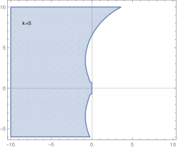
(e) Order five method.

Figure 1: Stability regions for fixed stepsize Limm methods of orders one through five. Orders one and two are $A$-stable, and orders three to five are $A(\phi)$-stable with $\phi$’s listed in Table 1.

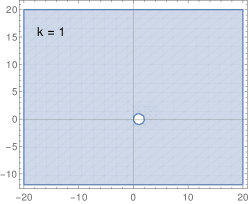
(a) Order one method.

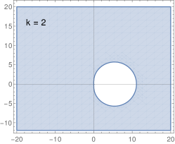
(b) Order two method.

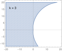
(c) Order three method.

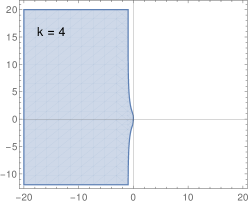
(d) Order four method.

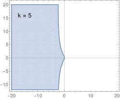
(e) Order five method.

Figure 2: Stability regions for fixed stepsize Limm-w methods of orders one through five. Orders one and two are $A$-stable, and orders three to five are $A(\phi)$-stable with $\phi$’s listed in Table 1.

Table 1: Characteristics of $k$-step fixed stepsize Limm, Limm-w, BDF, and explicit/implicit Adams methods for $k=1,\dots,5$. Implicit Adams methods are of order $k+1$; all others are of order $k$. For Limm and Limm-w, stability angles are computed from (46), and error constants are computed as in (51).

$\begin{array}[]{c|c|ccccc}&$k$&1&2&3&4&5\\ \hline\cr\hbox{\multirowsetup\text{explicit Adams}}&\text{A($\phi$)-stability angle}&\text{n/a}&\text{n/a}&\text{n/a}&\text{n/a}&\text{n/a}\\ &\text{Error constant}&0.5&0.416667&0.375&0.348611&0.329861\\ \hline\cr\hbox{\multirowsetup\text{implicit Adams}}&\text{A($\phi$)-stability angle}&90.&\text{n/a}&\text{n/a}&\text{n/a}&\text{n/a}\\ &\text{Error constant}&0.083333&0.041666&0.026389&0.01875&0.014269\\ \hline\cr\hbox{\multirowsetup\text{BDF}}&\text{A($\phi$)-stability angle}&90.&90.&86.03&73.35&51.84\\ &\text{Error constant}&0.5&0.333333&0.25&0.2&0.166667\\ \hline\cr\hbox{\multirowsetup\text{\sc Limm}}&\text{A($\phi$)-stability angle}&90.&90.&87.7849&78.0742&72.9999\\ &\text{Error constant}&0.5&0.222222&0.167344&0.204625&0.217405\\ \hline\cr\hbox{\multirowsetup\text{\sc Limm-w}}&\text{A($\phi$)-stability angle}&90.&90.&87.3899&77.9101&70.3168\\ &\text{Error constant}&0.5&0.424915&0.403238&0.380873&0.365325\end{array}$

Table 2: Exact coefficients for $k$-step fixed stepsize Limm methods of order $k$, for $k=1\dots 5$.

$\begin{array}[]{c|cc}i&-1&0\\ \hline\cr\alpha_{i}&1&-1\\ \beta_{i}&0&1\\ \mu_{i}&1&-1\\ \end{array}$

(a) Limm 1-step order 1 coefficients.

$\begin{array}[]{c|ccc}i&-1&0&1\\ \hline\cr\alpha_{i}&1&-\frac{4}{3}&\frac{1}{3}\\ \beta_{i}&0&\frac{2}{3}&0\\ \mu_{i}&\frac{2}{3}&-\frac{2}{3}&0\\ \end{array}$

(b) Limm 2-step order two coefficients.

$\begin{array}[]{c|cccc}i&-1&0&1&2\\ \hline\cr\alpha_{i}&1&-\frac{67569925}{40220258}&\frac{77233903}{99562899}&-\frac{383355371802341}{4004445485007942}\\ \beta_{i}&0&\frac{6}{11}&-\frac{56091046951621340}{198220051507893129}&\frac{30378060674886581}{198220051507893129}\\ \mu_{i}&\frac{3082752052157006}{6006668227511913}&-\frac{30378060674886581}{66073350502631043}&\frac{19781424978365126}{198220051507893129}&-\frac{30378060674886581}{198220051507893129}\\ \end{array}$

(c) Limm 3-step order three coefficients.

$\begin{array}[]{c|cc}i&-1&0\\ \hline\cr\alpha_{i}&1&-\frac{60010656}{28439311}\\ \beta_{i}&0&\frac{12}{25}\\ \mu_{i}&\frac{6044411368232668137128215}{12447162528941684828131512}&-\frac{60023632933941523627586873}{103726354407847373567762600}\\ \hline\cr i&1&2\\ \hline\cr\alpha_{i}&\frac{71006953}{40099309}&-\frac{345107661}{454781887}\\ \beta_{i}&-\frac{829829410576978812863115039}{1140989898486321109245388600}&\frac{133675753843217938307088979}{142623737310790138655673575}\\ \mu_{i}&\frac{194551206099828504610038241}{285247474621580277311347150}&-\frac{2829520362862954765370488571}{3422969695458963327736165800}\\ \hline\cr i&3&\text{}\\ \hline\cr\alpha_{i}&\frac{50927106883029008210353}{518631772039236867838813}&\text{}\\ \beta_{i}&-\frac{271157550073699750683379121}{1140989898486321109245388600}&\text{}\\ \mu_{i}&\frac{271157550073699750683379121}{1140989898486321109245388600}&\text{}\\ \end{array}$

(d) Limm 4-step order 4 coefficients.

$\begin{array}[]{c|cc}i&-1&0\\ \hline\cr\alpha_{i}&1&-\frac{104367911}{41202283}\\ \beta_{i}&0&\frac{60}{137}\\ \mu_{i}&\frac{322638273004961021870227746746423}{712722768713639590268860359964200}&-\frac{31175917409117421775097382197076197}{48821509656884311933416934657547700}\\ \hline\cr i&1&2\\ \hline\cr\alpha_{i}&\frac{59680231}{21017185}&-\frac{97736124}{57440479}\\ \beta_{i}&-\frac{1740570722762351776400683674709186511}{1220537741422107798335423366438692500}&\frac{487813399545245689582675417708028617}{203422956903684633055903894406448750}\\ \mu_{i}&\frac{1717451252646034545185780351980957211}{1220537741422107798335423366438692500}&-\frac{2669383545787015283771247804743841377}{1220537741422107798335423366438692500}\\ \hline\cr i&3&4\\ \hline\cr\alpha_{i}&\frac{19515650}{39801941}&-\frac{188732392210474496577705869057}{1979785468648998861857945444345}\\ \beta_{i}&-\frac{25562879042079908014978668038159641}{21412942831966803479568830990152500}&\frac{157267484617875282653199076556264173}{610268870711053899167711683219346250}\\ \mu_{i}&\frac{426670615738191742376152898428305157}{348725068977745085238692390411055000}&-\frac{157267484617875282653199076556264173}{610268870711053899167711683219346250}\\ \end{array}$

(e) Limm-w 5-step order 5 coefficients.

Table 3: Exact coefficients for $k$-step fixed stepsize Limm-w methods of order $k$, for $k=1\dots 5$.

$\begin{array}[]{c|cc}i&-1&0\\ \hline\cr\alpha_{i}&1&-1\\ \beta_{i}&0&1\\ \mu_{i}&1&-1\\ \end{array}$

(a) Limm-w 1-step order 1 coefficients.

$\begin{array}[]{c|ccc}i&-1&0&1\\ \hline\cr\alpha_{i}&1&-\frac{146619050}{133414177}&\frac{13204873}{133414177}\\ \beta_{i}&0&\frac{193518829}{133414177}&-\frac{73309525}{133414177}\\ \mu_{i}&\frac{73309525}{133414177}&-\frac{146619050}{133414177}&\frac{73309525}{133414177}\\ \end{array}$

(b) Limm-w 2-step order two coefficients.

$\begin{array}[]{c|cccc}i&-1&0&1&2\\ \hline\cr\alpha_{i}&1&-\frac{192592391}{118869921}&\frac{41981416}{61945353}&-\frac{5229175002546}{90906657005273}\\ \beta_{i}&0&\frac{16233524076078647}{9817918956569484}&-\frac{4193351041739980}{2454479739142371}&\frac{4833530710149845}{9817918956569484}\\ \mu_{i}&\frac{4833530710149845}{9817918956569484}&-\frac{4833530710149845}{3272639652189828}&\frac{4833530710149845}{3272639652189828}&-\frac{4833530710149845}{9817918956569484}\\ \end{array}$

(c) Limm-w 3-step order three coefficients.

$\begin{array}[]{c|cc}i&-1&0\\ \hline\cr\alpha_{i}&1&-\frac{68547635}{35752838}\\ \beta_{i}&0&\frac{136586035293284691}{70863342514650928}\\ \mu_{i}&\frac{719593273725529014067099}{1590107007076830596400464}&-\frac{719593273725529014067099}{397526751769207649100116}\\ \hline\cr i&1&2\\ \hline\cr\alpha_{i}&\frac{332147775}{246829693}&-\frac{120323842}{247754257}\\ \beta_{i}&-\frac{4675749204985773774031537}{1590107007076830596400464}&\frac{3052167106160890365719135}{1590107007076830596400464}\\ \mu_{i}&\frac{2158779821176587042201297}{795053503538415298200232}&-\frac{719593273725529014067099}{397526751769207649100116}\\ \hline\cr i&3&\text{}\\ \hline\cr\alpha_{i}&\frac{11382486133370227314625}{198763375884603824550058}&\text{}\\ \beta_{i}&-\frac{719593273725529014067099}{1590107007076830596400464}&\text{}\\ \mu_{i}&\frac{719593273725529014067099}{1590107007076830596400464}&\text{}\\ \end{array}$

(d) Limm-w 4-step order 4 coefficients.

$\begin{array}[]{c|cc}i&-1&0\\ \hline\cr\alpha_{i}&1&-\frac{170476503}{75237041}\\ \beta_{i}&0&\frac{3317715388830682274181888772466725}{1533160577078234002169550303186624}\\ \mu_{i}&\frac{659152962863648794216719015147251}{1533160577078234002169550303186624}&-\frac{3295764814318243971083595075736255}{1533160577078234002169550303186624}\\ \hline\cr i&1&2\\ \hline\cr\alpha_{i}&\frac{124149029}{52265116}&-\frac{53697673}{39342191}\\ \beta_{i}&-\frac{3387422206381293505203420155442595}{766580288539117001084775151593312}&\frac{294683351120793575703659865634035}{63881690711593083423731262632776}\\ \mu_{i}&\frac{3295764814318243971083595075736255}{766580288539117001084775151593312}&-\frac{3295764814318243971083595075736255}{766580288539117001084775151593312}\\ \hline\cr i&3&4\\ \hline\cr\alpha_{i}&\frac{67073128}{206463953}&-\frac{2219582774479398588921363466455}{31940845355796541711865631316388}\\ \beta_{i}&-\frac{1632980052046035774065588376123413}{766580288539117001084775151593312}&\frac{659152962863648794216719015147251}{1533160577078234002169550303186624}\\ \mu_{i}&\frac{3295764814318243971083595075736255}{1533160577078234002169550303186624}&-\frac{659152962863648794216719015147251}{1533160577078234002169550303186624}\\ \end{array}$

(e) Limm-w 5-step order 5 coefficients.

8 Variable Stepsize and Variable Order Implementation

In this section we discuss the details necessary to build an efficient self-starting variable stepsize and variable order implementation of Limm methods. Following [20, Chapter III.7], a key component required for adapting stepsize and order is an estimate $e^{(k,h)}_{n+1}$ of the local truncation error when the solution $y_{n+1}$ is computed with an order $k$ Limm scheme and step size $h_{n}$. Based on this error estimate one can determine whether to accept or reject the current step, and can estimate the optimal stepsize for a method of order $k$ using:

(49) $$h_{\text{opt}}^{(k)}=h_{n}\,\|e^{(k,h)}_{n+1}\|^{-1/(k+1)}.$$

To determine when a change of method order is needed, we further require the error estimates $e^{(k-1,h)}_{n+1}$ and $e^{(k+1,h)}_{n+1}$ for the order $k-1$ and $k+1$ methods, respectively. Then, we can select for the next step the method order which gives the best balance between a low estimated error and a large optimal timestep.

In traditional linear multistep methods [20, Chapter III.7] a Taylor expansion reveals that

(50) $$e^{(k,h)}_{n+1}=C_{k}(\bm{c})\,h_{n}^{k+1}\,y^{(k+1)}(t_{n+1})+\mathcal{O}\left(h_{n}^{k+2}\right),$$

where $C_{k}(\bm{c})$ is the method error coefficient as a function of the stepsize ratios $\bm{c}=[c_{i}]_{i=-1}^{k}$ (6), derived from residuals on the $k+1$ order conditions. In the Limm case different trees in the B-series expansion contribute differently to the $\mathcal{O}(h_{n}^{k+1})$ error term in (50), as can be seen from (7c)–(7d). In order to build practical error estimators we will use an expansion of the form (50) with our error constant computed from the two residuals (45):

(51) $$C_{k}(\bm{c})=\frac{1}{(k+1)!}\max\left(\left|\rho_{k+1,a}(\bm{c})\right|,\,\left|\rho_{k+1,a}(\bm{c})+\rho_{k+1,b}(\bm{c})\right|\right),$$

where the sum of the residuals is used because, for Limm, (45b) always appears on trees alongside (45a), as described in the observations below (19). We use past solutions for $y_{n+1},\dots,y_{n-k}$ to approximate the $(k+1)$-st time derivative of the solution via divided differences:

(52) $$\delta^{k+1}y\left[t_{n+1},\dots,t_{n-k}\right]=\frac{y^{(k+1)}(\xi)}{(k+1)!},\quad\xi\in[t_{n-k},t_{n+1}].$$

Putting together equations (50), (51), and (52) we arrive at the following estimate for the local error.

Definition 8.1 (Local error estimate).

For a $k$-step order $k$ Limm method a practical local truncation error estimate is:

(53) $$e^{(k,h)}_{n+1}=(k+1)!\,C_{k}(\bm{c})\,h_{n}^{k+1}\,\delta^{k+1}y\left[t_{n+1},\dots,t_{n-k}\right],$$

using method error coefficient $C_{k}(\bm{c})$ (51), the current stepsize $h_{n}$, and the $(k+1)$-st order divided difference of the solution at $t_{n+1},\dots,t_{n-k}$. Due to (51), (53) may slightly overestimate the local errors in the asymptotic regime.

This error estimate is convenient for our purpose, as we can compute estimates for methods of order $k-1$ and $k+1$ by simply using their error coefficients and changing the order of the divided difference. Note that the divided difference of order $k+1$ requires $y_{n+1}$ and a history of $k+1$ values of $y_{n},\dots,y_{n-k}$, whereas the $k$-step Limm method only requires a history of $k$ values of $y$ in order to compute $y_{n+1}$. Divided differences for the higher order methods require storing additional past solution values.

Instead of building divided differences at each step from the history of solutions, it is more efficient to maintain a history of the divided differences and build new ones using the following formulas (similar to updating the Nordsieck vector in a variety of multistep codes [6, 3, 27]). First, after computing $y_{n+1}$ via the Limm method, we produce the $(k+1)$-st divided difference as follows:

(54) $$\delta^{k+1}y\left[t_{n+1},\dots,t_{n-k}\right]=\frac{y_{n+1}-y_{n}}{\prod_{j=0}^{k}\sum_{l=0}^{j}(t_{n+1-l}-t_{n-l})}-\sum_{i=1}^{k}\frac{\delta^{i}y\left[t_{n},\dots,t_{n-i}\right]}{\prod_{j=i}^{k}\sum_{l=0}^{j}(t_{n+1-l}-t_{n-l})}.$$

Then, through direct application of the recursive definition, one computes the updated values of order $k$ and $k+2$ divided differences.

(55a) $$\delta^{k}y\left[t_{n+1},\dots,t_{n-k+1}\right]=\delta^{k}y\left[t_{n},\dots,t_{n-k}\right]+\sum_{j=0}^{k}h_{n-j}\,\delta^{k+1}y\left[t_{n+1},\dots,t_{n-k}\right],$$

(55b) $$\delta^{k+2}y\left[t_{n+1},\dots,t_{n-k-1}\right]=\frac{\delta^{k+1}y\left[t_{n+1},\dots,t_{n-k}\right]-\delta^{k+1}y\left[t_{n},\dots,t_{n-k-1}\right]}{\sum_{j=0}^{k+1}h_{n-j}}.$$

Together, this requires saving divided differences of orders $$0,\dots,k+2 y_{n} k+2 1,\dots,k-1$$ at each timestep (with the order 0 coming from the direct use of in (54), and order needed in the event we choose to use a higher order method for the next step). Order differences can be updated via repeated application of (55a):

(55c) $$\delta^{i-1}y\left[t_{n+1},\dots,t_{n-i+2}\right]=\delta^{i-1}y\left[t_{n},\dots,t_{n-i+1}\right]+\sum_{j=0}^{i-1}h_{n-j}\delta^{i}y\left[t_{n+1},\dots,t_{n-i+1}\right].$$

To avoid the redundant saving of both the history of solution values and of divided differences, one can reformulate the Limm method (5) in terms of divided differences:

(56) $$\begin{split}&\left(\mathbf{I}-h_{n}\,\mu_{-1}(\bm{c})\,\mathbf{J}_{n}\right)y_{n+1}=-\sum_{i=0}^{k-1}h_{n}^{i}\,\widehat{\alpha}_{i}(\bm{c})\,\delta^{i}y\left[t_{n},\dots,t_{n-i}\right]\\ &\qquad+h\,\mathbf{J}_{n}\,\sum_{i=0}^{k-1}h_{n}^{i}\,\widehat{\mu}_{i}(\bm{c})\,\delta^{i}y\left[t_{n},\dots,t_{n-i}\right]+h_{n}\,\sum_{i=0}^{k-1}h_{n}^{i}\,\widehat{\beta}_{i}(\bm{c})\,\delta^{i}f\left[t_{n},\dots,t_{n-i}\right],\end{split}$$

where $\delta^{i}f\left[t_{n},\dots,t_{n-i}\right]$ are divided differences constructed from evaluations of the right-hand side function $f(t_{n},y_{n})$ evaluated at $(t_{n},y_{n})$, and $\widehat{\alpha}_{i}$, $\widehat{\mu}_{i}$, $\widehat{\beta}_{i}$ are transformed coefficients (as functions of the timestep ratios). The transformed coefficients can be computed from the original method coefficients as

(57) $$\widehat{\alpha}_{i}(\bm{c}) =(-1)^{i}\sum_{j=i}^{k-1}\alpha_{j}(\bm{c})\prod_{l=1}^{i}\sum_{m=l}^{j}(c_{m}-c_{m-1}),$$

(58) $$\widehat{\beta}_{i}(\bm{c}) =(-1)^{i}\sum_{j=i}^{k-1}\beta_{j}(\bm{c})\prod_{l=1}^{i}\sum_{m=l}^{j}(c_{m}-c_{m-1}),$$

(59) $$\widehat{\mu}_{i}(\bm{c}) =(-1)^{i}\sum_{j=i}^{k-1}\mu_{j}(\bm{c})\prod_{l=1}^{i}\sum_{m=l}^{j}(c_{m}-c_{m-1}).$$

Remark 8.2 (The first step).

The first step of integration requires additional care. Even starting with a one-step order one method requires an order two divided difference for error estimation (and a difference of order three for estimation of the order two method’s error). We initialize our divided differences as follows:

$$\delta^{0}y[t_{0}] =y_{0},\quad\delta^{1}y\left[t_{0}\right]\approx f_{0}.$$

Then, following the computation of $y_{1}$, we approximate the next divided differences

$$\delta^{2}y\left[t_{1},t_{0}\right] \approx\left((y_{1}-y_{0})/h_{0}-f_{0}\right)/\left(2h_{0}\right),\quad\delta^{3}y\left[t_{1},t_{0}\right]\approx\left(\delta^{2}y\left[t_{1},t_{0}\right]-\mathbf{J}_{0}f_{0}\right)/\left(3h_{0}\right).$$

Remark 8.3 (Stability for variable stepsize methods).

Evaluating the stability properties of variable stepsize multistep methods is challenging (see [8, 7, 9, 19] for analysis of variable stepsize BDF methods). Specifically, explicit formulas for the bounds $\omega_{\rm min}$ and $\omega_{\rm max}$ in Theorem 5.1 that ensure stability for a general multistep methods are not available. Since an in-depth analysis is outside the scope of the current work, we follow the best practices of other variable stepsize multistep implementations [20, Section III.5], by ensuring the base fixed stepsize method (from which the variable stepsize one is derived) is stable, and limiting stepsize increases to only occur after $k$ successful steps at the current stepsize. Specifically, we allow step changes occur after only $k+1$ successful steps have been taken with the current stepsize.

9 Numerical Results

In this section we present numerical results for Limm methods including both convergence and performance experiments. First, we demonstrate the convergence order of the fixed stepsize Limm and Limm-w methods, then we examine the performance of the self-starting variable stepsize and variable order implementation of the Limm methods which was detailed in section 8.

The convergence tests use fixed stepsize implementations of Limm and Limm-w, with the built-in Matlab time integrator ode15s used as a starter method. For the performance tests, our primary point of comparison is the BDF methods [20, Section III.1], one of the most widely used families of implicit multistep methods. We use a self-starting variable stepsize and order implementation of BDF built in the same framework as the Limm implementation, using the same error controller and also the error estimator from definition 8.1. For comparison we include results for SDIRK4a [21, Section IV.6] (a 5-stage, fourth order singly diagonally implicit Runge-Kutta method) and RODAS4 [21, Section VI.4] (a 6-stage, fourth order Rosenbrock method) as examples of high-order single step implicit methods. The variable stepsize Limm-(w) and BDF implementations, along with the SDIRK4a and RODAS4 methods can be found in our MatlODE package [44], in the limm_dev branch. We also provide comparisons against the Matlab built-in ode15s in both BDF and NDF modes.

Each time integrator is tested by sweeping through the same series of tolerances from $10^{-2},10^{-3},...,10^{-10}$, with equal relative and absolute tolerances. When GMRES is used for linear system solves, it uses a tolerance that is one tenth of the integrator tolerance. All tests are performed in Matlab (version 2019a) on a workstation with dual Intel Xeon E5-2650 v3 processors with 20 cores (40 threads) and 128GB of memory. Test problems are drawn from the ODE Test Problems package [31], which contains Matlab implementations of a variety of ODEs and PDEs suitable for testing time integrators. Reference solutions are obtained by applying the Matlab built-in ode15s integrator when full Jacobians are available, or an implementation of RODAS4 using GMRES when only Jacobian-vector products are available; both are applied with the tightest possible tolerance of $100$ times the machine precision.

9.1 Convergence: Lorenz-96 ODE

To test the convergence order of the fixed stepsize Limm and Limm-w methods, we use the Lorenz-96 problem [23], a system of nonlinear ODEs defined as

(60) $$\frac{\text{d}x_{i}}{\text{d}t}=\left(x_{i+1}-x_{i-2}\right)x_{i-1}-x_{i}+F(t),\quad i=1,\dots,N,$$

with periodic boundary conditions $x_{N+1}=x_{1}$, $x_{0}=x_{N}$, $x_{-1}=x_{N-1}$ and forcing function $F(t)=8+4\cos\left(3\pi t\right)$. We select $N=40$, and timespan $t\in\left[0,0.5\right]$.

Figure 3 shows the convergence results for Limm orders 1-5 as solid lines, and for Limm-w orders 1-5 as dashed lines. The legend contains the slopes of the linear interpolants for each test, demonstrating that each method achieves its theoretical order. Limm-w shows slightly smaller total errors.

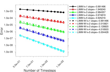
Figure 3: Fixed stepsize results for the Lorenz-96 problem (60) showing the orders of convergence for Limm-w (dashed lines) and Limm (solid lines) methods for orders 1-5.

9.2 Performance: Gray–Scott reaction-diffusion model

We run performance comparisons using the Gray–Scott reaction-diffusion model, which describes a two species chemical reactions with retirement [17, 18]:

$$U+2V \rightarrow 3V$$

$$V \rightarrow P.$$

(61) $$\frac{\partial u}{\partial t}=\varepsilon_{1}\Delta u-uv^{2}+F(1-u),\qquad\frac{\partial v}{\partial t}=\varepsilon_{2}\Delta v+uv^{2}-(F+k)v,$$

where $\varepsilon_{1}=0.2$ and $\varepsilon_{2}=0.1$ are diffusion rates, and $F=0.04$ and $k=0.06$ are reaction rates. We use a second order finite difference spatial discretization with periodic boundary conditions on a $128\times 128$ 2D grid, which brings (61) to ODE form (1) with $N=2\times 128\times 128$. The simulation time interval is $t\in[0,2]$.

Results on the Gray–Scott model are given in Figure 4 for our implementations of Limm, Limm-w, BDF, SDIRK4a, RODAS4, as well as for the ode15s implementations of BDF and NDF [38]. Because the full Jacobian is available, all methods use a direct $LU$-factorization, that is reused for methods requiring multiple linear solves per step. The error vs. timestep count results in Figure 4a reveal that all five multistep integrators achieve similar levels of error with similar numbers of timesteps, thus none of these multistep methods or implementations have a clear stability or error advantage over the others in this test. The one-step methods SDIRK4a and RODAS4 do show better errors with fewer timesteps, likely as a result of their greater flexibility in choosing timestep sizes. The CPU time comparison in Figure 4b reveals the advantage of the built-in ode15s implementations, as they benefit from a massive amount of software optimizations. Comparing the results for our implementation of multistep integrators, we can see a small performance advantage for Limm and Limm-w over the similar BDF implementation, due to the need for only one linear system solve per timestep. Given a similar level of software optimization, we might expect the Limm methods to hold the same advantage over the ode15s BDF implementation. The SDIRK4a and RODAS4 also show very good performance, due to the lower timestep count and reuse one $LU$-factorization per timestep.

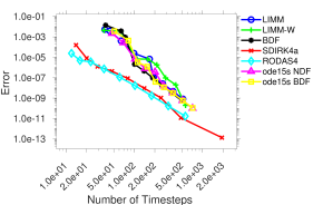
(a) Variable stepsize convergence results.

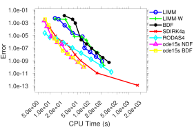
(b) Work-precision diagram.

Figure 4: Performance results for different integrators applied to the 2D Gray-Scott reaction-diffusion problem (61).

9.3 Performance: quasi-geostrophic model

Next, we compare method performance using the 1.5-layer quasi-geostrophic (QG) model [33], which provides a simplified representation of ocean dynamics:

(62) $$\displaystyle\frac{\partial q}{\partial t} =-\psi_{x}-\varepsilon J\left(\psi,q\right)-A\Delta^{3}\psi+2\pi\text{sin}\left(2\pi y\right),\qquad q=\Delta\psi-F\psi,$$

where $J\left(\psi,q\right)=\psi_{x}q_{y}-\psi_{y}q_{x}$, and $F=1600$, $\varepsilon=10^{-5}$ and $A=10^{-5}$ are constants. The implementation discretizes the system in terms of the stream function $\psi$, on the spatial domain $(x,y)\in[0,1]^{2}$, using second order central finite differences and homogeneous Dirichlet boundary conditions on a $127\times 127$ grid. Integration is performed over the time span $t\in\left[0,0.01\right]$. Due to the required solution of a Helmholtz equation, a portion of the QG Jacobian is dense; only Jacobian-vector products are available and all integrators use GMRES as linear solver, except for ode15s which cannot use iterative linear solvers. Instead, both BDF and NDF results for ode15s make use of a numerical Jacobian approximation.

Figure 5 shows errors versus timestep count and CPU times for Limm, Limm-w, BDF, SDIRK4a, RODAS4, and ode15s applied to the QG model. First, we notice the jagged behavior of both the Limm and BDF methods, especially at looser tolerances; this is an artifact of the variable order methods, where methods of lower order are preferred for their better stability. When the tolerances are tightened, the graphs smoothen, as the algorithm prefers the better asymptotic errors of the higher order methods. The Limm and Limm-w methods are particularly sensitive to this, possibly due to the use of GMRES, as inexact linear solves could degrade stability or lead to Limm order reduction. Despite this, Figure 5b shows that Limm retains its CPU time advantage over BDF, and also matches or outperforms RODAS4 and SDIRK4a for similar levels of error, as the small stability advantages that BDF, SDIRK and Rosenbrock methods have cannot overcome their larger cost per timestep. The built-in ode15s methods both provide very poor performance for this test case, as they do not support the use of direct Jacobian-vector products and are forced to build numerical Jacobian approximations to use with direct solves.

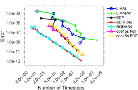
(a) Variable stepsize convergence results.

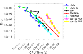
(b) Work-precision diagram.

Figure 5: Performance results for different integrators applied to the 1.5 layer QG model (62).

10 Conclusions

Classical implicit linear multistep methods require the solution of a nonlinear system of equations at each timestep. This work develops the Limm class of linearly implicit multistep methods, which only require the solution of one linear system per timestep. Order conditions for variable stepsize Limm methods of arbitrary order are constructed via Butcher trees and B-series operations. Order conditions for Limm-w schemes that can use arbitrary approximations of the Jacobian matrix are developed by direct series expansion. A Limm method has twice as many coefficients as a traditional linear multistep method (with the same number of steps), and this additional freedom enables the construction of methods with excellent accuracy and stability properties. We discuss the optimal design of Limm methods, and develop a set of $k$-step order $k$ Limm methods for $k=1,\dots,5$. We also discuss the details of a self-starting variable stepsize and variable order implementation of these Limm methods. Numerical experiments demonstrate the convergence at the theoretical orders for the fixed stepsize Limm methods. Moreover, our variable stepsize Limm implementation outperforms a comparable BDF implementation for nonlinear problems.

In the future, we intend to use the family of Limm-w methods to reuse the same Jacobian for multiple timesteps. Additionally, extension of Limm to use a Krylov subspace approximation of the Jacobian, as in Rosenbrock-Krylov or exponential-Krylov methods is underway, which will directly account for errors coming from Krylov-based iterative linear solvers in the order conditions of the time integrator.

Appendix A Variable stepsize Limm coefficients

Tables 4 – 9 contain the variable stepsize coefficient expressions for Limm methods of order 1-5, parameterized by the $c_{i}$’s defined in (6), and the constant coeffcients.

Table 4: Limm 1-step order 1 coefficients.

$\begin{array}[]{c|cc}i&-1&0\\ \hline\cr\alpha_{i}&1&-1\\ \beta_{i}&0&1\\ \mu_{i}&1&-1\\ \end{array}$

Table 5: Limm 2-step order 2 variable stepsize coefficients.

$\begin{array}[]{c|ccc}i&-1&0&1\\ \hline\cr\alpha_{i}&1&-\frac{4}{3}&\frac{1}{3}\\ \beta_{i}&0&\frac{2}{3}&-\beta_{0}+\left(\alpha_{0}+1\right)c_{1}+1\\ \mu_{i}&\frac{1}{2}\left(1-\left(\alpha_{0}+1\right)c_{1}^{2}\right)&\frac{1}{2}\left(-2\beta_{0}+\left(\alpha_{0}+1\right)c_{1}^{2}+2\left(\alpha_{0}+1\right)c_{1}+1\right)&\beta_{0}+\left(\alpha_{0}+1\right)\left(-c_{1}\right)-1\\ \end{array}$

Table 6: Limm 3-step order 3 variable stepsize coefficients.

$\begin{array}[]{c|l}\hline\cr\alpha_{-1}&1\\ \beta_{-1}&0\\ \mu_{-1}&\left[\alpha_{1}c_{1}^{3}-3c_{1}\left(\left(\alpha_{0}+\alpha_{1}+1\right)c_{2}^{2}-1\right)+2\left(\alpha_{0}+\alpha_{1}+1\right)c_{2}^{3}+2\right]/\left(6\left(c_{1}+1\right)\right)\\ \hline\cr\alpha_{0}&-67569925/40220258\\ \beta_{0}&6/11\\ \mu_{0}&-\left[-3c_{1}\left(-2\beta_{0}+\left(\alpha_{0}+\alpha_{1}+1\right)c_{2}^{2}+2\left(\alpha_{0}+\alpha_{1}+1\right)c_{2}+1\right)+\alpha_{1}c_{1}^{3}+3\alpha_{1}c_{1}^{2}+2\left(\alpha_{0}+\alpha_{1}+1\right)c_{2}^{3}+3\left(\alpha_{0}+\alpha_{1}+1\right)c_{2}^{2}-1\right]/\left(6c_{1}\right)\\ \hline\cr\alpha_{1}&77233903/99562899\\ \beta_{1}&\left[-\alpha_{1}c_{1}^{3}+3\alpha_{1}c_{2}^{2}c_{1}-2\left(\alpha_{0}+\alpha_{1}+1\right)c_{2}^{3}+3\left(\beta_{0}-1\right)c_{2}^{2}+1\right]/\left(3\left(c_{1}^{2}-c_{2}^{2}\right)\right)\\ \mu_{1}&\left[3c_{1}^{2}\left(c_{2}^{2}\left(\alpha_{0}-2\beta_{0}+3\right)+2\left(\alpha_{0}+\alpha_{1}+1\right)c_{2}^{3}-1\right)+c_{1}\left(4\left(\alpha_{0}+\alpha_{1}+1\right)c_{2}^{3}-6\left(\beta_{0}-1\right)c_{2}^{2}-2\right)-2\left(\alpha_{0}+\alpha_{1}+1\right)c_{2}^{5}\right.\\ &\left.-3\left(\alpha_{0}+\alpha_{1}+1\right)c_{2}^{4}-4\alpha_{1}c_{1}^{3}c_{2}^{2}-\alpha_{1}c_{1}^{4}+c_{2}^{2}\right]/\left(6c_{1}\left(c_{1}+1\right)\left(c_{1}-c_{2}\right)\left(c_{1}+c_{2}\right)\right)\\ \hline\cr\alpha_{2}&-383355371802341/4004445485007942\\ \beta_{2}&-\left[3c_{1}^{2}\left(\beta_{0}+\left(\alpha_{0}+\alpha_{1}+1\right)\left(-c_{2}\right)-1\right)+2\alpha_{1}c_{1}^{3}+\left(\alpha_{0}+\alpha_{1}+1\right)c_{2}^{3}+1\right]/\left(3\left(c_{1}^{2}-c_{2}^{2}\right)\right)\\ \mu_{2}&\left[3c_{1}^{2}\left(\beta_{0}+\left(\alpha_{0}+\alpha_{1}+1\right)\left(-c_{2}\right)-1\right)+2\alpha_{1}c_{1}^{3}+\left(\alpha_{0}+\alpha_{1}+1\right)c_{2}^{3}+1\right]/\left(3\left(c_{1}^{2}-c_{2}^{2}\right)\right)\\ \end{array}$

Table 7: Limm 4-step order 4 variable stepsize coefficients.

$\begin{array}[]{c|l}\hline\cr\alpha_{-1}&1\\ \beta_{-1}&0\\ \mu_{-1}&\left[-\alpha_{1}c_{1}^{4}+2\alpha_{1}c_{2}c_{1}^{3}+2c_{1}\left(\alpha_{2}c_{2}^{3}-3c_{2}\left(\left(\alpha_{0}+\alpha_{1}+\alpha_{2}+1\right)c_{3}^{2}-1\right)+2\left(\alpha_{0}+\alpha_{1}+\alpha_{2}+1\right)c_{3}^{3}+2\right)-\alpha_{2}c_{2}^{4}-3\left(\alpha_{0}+\alpha_{1}+\alpha_{2}+1\right)c_{3}^{4}+4c_{2}\left(\left(\alpha_{0}+\alpha_{1}+\alpha_{2}+1\right)c_{3}^{3}+1\right)+3\right]/\left(12\left(c_{1}+1\right)\left(c_{2}+1\right)\right)\\ \hline\cr\alpha_{0}&-60010656/28439311\\ \beta_{0}&12/25\\ \mu_{0}&\left[-2c_{1}\left(-3c_{2}\left(-2\beta_{0}+\left(\alpha_{0}+\alpha_{1}+\alpha_{2}+1\right)c_{3}^{2}+2\left(\alpha_{0}+\alpha_{1}+\alpha_{2}+1\right)c_{3}+1\right)+\alpha_{2}c_{2}^{3}+3\alpha_{2}c_{2}^{2}+2\left(\alpha_{0}+\alpha_{1}+\alpha_{2}+1\right)c_{3}^{3}+3\left(\alpha_{0}+\alpha_{1}+\alpha_{2}+1\right)c_{3}^{2}-1\right)+\alpha_{1}c_{1}^{4}-2\alpha_{1}\left(c_{2}-1\right)c_{1}^{3}-6\alpha_{1}c_{2}c_{1}^{2}\right.\\ &\left.+3\alpha_{0}c_{3}^{4}+4\alpha_{0}c_{3}^{3}+3\alpha_{1}c_{3}^{4}+4\alpha_{1}c_{3}^{3}+\alpha_{2}c_{2}^{4}+3\alpha_{2}c_{3}^{4}+2\alpha_{2}c_{2}^{3}+4\alpha_{2}c_{3}^{3}-2c_{2}\left(2\left(\alpha_{0}+\alpha_{1}+\alpha_{2}+1\right)c_{3}^{3}+3\left(\alpha_{0}+\alpha_{1}+\alpha_{2}+1\right)c_{3}^{2}-1\right)+3c_{3}^{4}+4c_{3}^{3}+1\right]/\left(12c_{1}c_{2}\right)\\ \hline\cr\alpha_{1}&71006953/40099309\\ \beta_{1}&\left[4c_{2}^{2}\left(\alpha_{1}c_{1}^{3}-3\alpha_{1}c_{3}^{2}c_{1}+2\left(\alpha_{0}+\alpha_{1}+\alpha_{2}+1\right)c_{3}^{3}-3\left(\beta_{0}-1\right)c_{3}^{2}-1\right)+\alpha_{2}c_{2}^{5}+\alpha_{2}c_{3}c_{2}^{4}-8\alpha_{2}c_{3}^{2}c_{2}^{3}-c_{2}\left(3\alpha_{1}c_{1}^{4}-4\alpha_{1}c_{3}c_{1}^{3}+\left(\alpha_{0}+\alpha_{1}+\alpha_{2}+1\right)c_{3}^{4}+4c_{3}+3\right)\right.\\ &\left.-c_{3}\left(3\alpha_{1}c_{1}^{4}-4\alpha_{1}c_{3}c_{1}^{3}+\left(\alpha_{0}+\alpha_{1}+\alpha_{2}+1\right)c_{3}^{4}+4c_{3}+3\right)\right]/\left(12\left(c_{1}-c_{2}\right)\left(c_{1}-c_{3}\right)\left(c_{2}c_{3}+c_{1}\left(c_{2}+c_{3}\right)\right)\right)\\ \mu_{1}&-\left[-2c_{1}^{2}\left(-3c_{2}^{2}\left(c_{3}^{2}\left(\alpha_{0}+\alpha_{2}-2\beta_{0}+3\right)+2\left(\alpha_{0}+\alpha_{1}+\alpha_{2}+1\right)c_{3}^{3}-1\right)+\alpha_{2}c_{2}^{4}+\alpha_{2}c_{3}\left(4c_{3}+1\right)c_{2}^{3}-c_{2}\left(\left(\alpha_{0}+\alpha_{1}+\alpha_{2}+1\right)c_{3}^{3}-3c_{3}-2\right)+2c_{3}\left(c_{3}+1\right)\left(\left(\alpha_{0}+\alpha_{1}+\alpha_{2}+1\right)c_{3}^{3}+1\right)\right)\right.\\ &\left.+c_{1}\left(4c_{2}^{2}\left(2\left(\alpha_{0}+\alpha_{1}+\alpha_{2}+1\right)c_{3}^{3}-3\left(\beta_{0}-1\right)c_{3}^{2}-1\right)+\alpha_{2}c_{2}^{5}+\alpha_{2}c_{3}\left(c_{3}+1\right)c_{2}^{4}-6\alpha_{2}c_{3}^{2}c_{2}^{3}-c_{2}\left(4\left(\alpha_{0}+\alpha_{1}+\alpha_{2}+1\right)c_{3}^{5}+7\left(\alpha_{0}+\alpha_{1}+\alpha_{2}+1\right)c_{3}^{4}-2c_{3}^{2}+4c_{3}+3\right)\right.\right.\\ &\left.\left.+3c_{3}\left(c_{3}+1\right)\left(\left(\alpha_{0}+\alpha_{1}+\alpha_{2}+1\right)c_{3}^{4}-1\right)\right)+\alpha_{1}\left(c_{3}^{2}+c_{3}+c_{2}\right)c_{1}^{5}-\alpha_{1}c_{2}\left(2c_{2}-\left(c_{3}-2\right)c_{3}\right)c_{1}^{4}-2\alpha_{1}c_{2}\left(4c_{2}-1\right)c_{3}^{2}c_{1}^{3}\right.\\ &\left.+c_{2}c_{3}^{2}\left(\alpha_{2}c_{2}^{4}+2\alpha_{2}c_{2}^{3}-2c_{2}\left(2\left(\alpha_{0}+\alpha_{1}+\alpha_{2}+1\right)c_{3}^{3}+3\left(\alpha_{0}+\alpha_{1}+\alpha_{2}+1\right)c_{3}^{2}-1\right)+3\left(\alpha_{0}+\alpha_{1}+\alpha_{2}+1\right)c_{3}^{4}+4\left(\alpha_{0}+\alpha_{1}+\alpha_{2}+1\right)c_{3}^{3}+1\right)\right]\\ &/\left(12c_{1}\left(c_{1}+1\right)\left(c_{1}-c_{2}\right)\left(c_{1}-c_{3}\right)\left(c_{2}c_{3}+c_{1}\left(c_{2}+c_{3}\right)\right)\right)\\ \hline\cr\alpha_{2}&-345107661/454781887\\ \beta_{2}&\left[-4c_{1}^{2}\left(\alpha_{2}c_{2}^{3}-3\alpha_{2}c_{3}^{2}c_{2}+2\left(\alpha_{0}+\alpha_{1}+\alpha_{2}+1\right)c_{3}^{3}-3\left(\beta_{0}-1\right)c_{3}^{2}-1\right)-\alpha_{1}c_{1}^{5}-\alpha_{1}c_{3}c_{1}^{4}+8\alpha_{1}c_{3}^{2}c_{1}^{3}+c_{1}\left(3\alpha_{2}c_{2}^{4}-4\alpha_{2}c_{3}c_{2}^{3}+\left(\alpha_{0}+\alpha_{1}+\alpha_{2}+1\right)c_{3}^{4}+4c_{3}+3\right)\right.\\ &\left.+c_{3}\left(3\alpha_{2}c_{2}^{4}-4\alpha_{2}c_{3}c_{2}^{3}+\left(\alpha_{0}+\alpha_{1}+\alpha_{2}+1\right)c_{3}^{4}+4c_{3}+3\right)\right]/\left(12\left(c_{1}-c_{2}\right)\left(c_{2}-c_{3}\right)\left(c_{2}c_{3}+c_{1}\left(c_{2}+c_{3}\right)\right)\right)\\ \mu_{2}&\left[-2c_{1}^{2}\left(-3c_{2}^{2}\left(c_{3}^{2}\left(\alpha_{0}+\alpha_{1}-2\beta_{0}+3\right)+2\left(\alpha_{0}+\alpha_{1}+\alpha_{2}+1\right)c_{3}^{3}-1\right)-2c_{2}\left(2\left(\alpha_{0}+\alpha_{1}+\alpha_{2}+1\right)c_{3}^{3}-3\left(\beta_{0}-1\right)c_{3}^{2}-1\right)+\alpha_{2}c_{2}^{4}+4\alpha_{2}c_{3}^{2}c_{2}^{3}\right.\right.\\ &\left.\left.+c_{3}^{2}\left(2\left(\alpha_{0}+\alpha_{1}+\alpha_{2}+1\right)c_{3}^{3}+3\left(\alpha_{0}+\alpha_{1}+\alpha_{2}+1\right)c_{3}^{2}-1\right)\right)+\alpha_{1}\left(c_{3}^{2}+c_{2}\right)c_{1}^{5}+\alpha_{1}\left(-2c_{2}^{2}+c_{3}\left(c_{3}+1\right)c_{2}+2c_{3}^{2}\right)c_{1}^{4}-2\alpha_{1}c_{2}c_{3}\left(3c_{3}+c_{2}\left(4c_{3}+1\right)\right)c_{1}^{3}\right.\\ &\left.+c_{1}\left(3\left(\alpha_{0}+\alpha_{1}+\alpha_{2}+1\right)c_{3}^{6}+4\left(\alpha_{0}+\alpha_{1}+\alpha_{2}+1\right)c_{3}^{5}+2\alpha_{2}c_{2}^{3}c_{3}^{2}+\alpha_{2}c_{2}^{4}\left(c_{3}-2\right)c_{3}+\alpha_{2}c_{2}^{5}+2c_{2}^{2}\left(\left(\alpha_{0}+\alpha_{1}+\alpha_{2}+1\right)c_{3}^{3}-3c_{3}-2\right)-c_{2}\left(4\left(\alpha_{0}+\alpha_{1}+\alpha_{2}+1\right)c_{3}^{5}+7\left(\alpha_{0}+\alpha_{1}+\alpha_{2}+1\right)c_{3}^{4}\right.\right.\right.\\ &\left.\left.\left.-2c_{3}^{2}+4c_{3}+3\right)+c_{3}^{2}\right)+c_{2}c_{3}\left(c_{3}+1\right)\left(\alpha_{2}c_{2}^{4}-4c_{2}\left(\left(\alpha_{0}+\alpha_{1}+\alpha_{2}+1\right)c_{3}^{3}+1\right)+3\left(\alpha_{0}+\alpha_{1}+\alpha_{2}+1\right)c_{3}^{4}-3\right)\right]/\left(12\left(c_{1}-c_{2}\right)c_{2}\left(c_{2}+1\right)\left(c_{2}-c_{3}\right)\left(c_{2}c_{3}+c_{1}\left(c_{2}+c_{3}\right)\right)\right)\\ \hline\cr\alpha_{3}&50927106883029008210353/518631772039236867838813\\ \beta_{3}&\left[4c_{1}^{2}\left(3c_{2}^{2}\left(\beta_{0}+\left(\alpha_{0}+\alpha_{1}+\alpha_{2}+1\right)\left(-c_{3}\right)-1\right)+2\alpha_{2}c_{2}^{3}+\left(\alpha_{0}+\alpha_{1}+\alpha_{2}+1\right)c_{3}^{3}+1\right)-\alpha_{1}c_{1}^{5}-\alpha_{1}c_{2}c_{1}^{4}+8\alpha_{1}c_{2}^{2}c_{1}^{3}+c_{1}\left(-\alpha_{2}c_{2}^{4}+4c_{2}\left(\left(\alpha_{0}+\alpha_{1}+\alpha_{2}+1\right)c_{3}^{3}+1\right)-3\left(\alpha_{0}+\alpha_{1}+\alpha_{2}+1\right)c_{3}^{4}+3\right)\right.\\ &\left.+c_{2}\left(-\alpha_{2}c_{2}^{4}+4c_{2}\left(\left(\alpha_{0}+\alpha_{1}+\alpha_{2}+1\right)c_{3}^{3}+1\right)-3\left(\alpha_{0}+\alpha_{1}+\alpha_{2}+1\right)c_{3}^{4}+3\right)\right]/\left(12\left(c_{1}-c_{3}\right)\left(c_{3}-c_{2}\right)\left(c_{2}c_{3}+c_{1}\left(c_{2}+c_{3}\right)\right)\right)\\ \mu_{3}&\left[-4c_{1}^{2}\left(3c_{2}^{2}\left(\beta_{0}+\left(\alpha_{0}+\alpha_{1}+\alpha_{2}+1\right)\left(-c_{3}\right)-1\right)+2\alpha_{2}c_{2}^{3}+\left(\alpha_{0}+\alpha_{1}+\alpha_{2}+1\right)c_{3}^{3}+1\right)+\alpha_{1}c_{1}^{5}+\alpha_{1}c_{2}c_{1}^{4}-8\alpha_{1}c_{2}^{2}c_{1}^{3}+c_{1}\left(\alpha_{2}c_{2}^{4}-4c_{2}\left(\left(\alpha_{0}+\alpha_{1}+\alpha_{2}+1\right)c_{3}^{3}+1\right)+3\left(\alpha_{0}+\alpha_{1}+\alpha_{2}+1\right)c_{3}^{4}-3\right)\right.\\ &\left.+c_{2}\left(\alpha_{2}c_{2}^{4}-4c_{2}\left(\left(\alpha_{0}+\alpha_{1}+\alpha_{2}+1\right)c_{3}^{3}+1\right)+3\left(\alpha_{0}+\alpha_{1}+\alpha_{2}+1\right)c_{3}^{4}-3\right)\right]/\left(12\left(c_{1}-c_{3}\right)\left(c_{3}-c_{2}\right)\left(c_{2}c_{3}+c_{1}\left(c_{2}+c_{3}\right)\right)\right)\\ \end{array}$

Table 8: Limm 5-step order 5 variable stepsize coefficients (part 1).

$\begin{array}[]{c|l}\hline\cr\alpha_{-1}&1\\ \beta_{-1}&0\\ \mu_{-1}&\left[3\alpha_{1}c_{1}^{5}-5\alpha_{1}\left(c_{2}+c_{3}\right)c_{1}^{4}+10\alpha_{1}c_{2}c_{3}c_{1}^{3}-5c_{1}\left(\alpha_{2}c_{2}^{4}-2\alpha_{2}c_{3}c_{2}^{3}-2c_{2}\left(\alpha_{3}c_{3}^{3}-3c_{3}\left(\left(\alpha_{0}+\alpha_{1}+\alpha_{2}+\alpha_{3}+1\right)c_{4}^{2}-1\right)+2\left(\alpha_{0}+\alpha_{1}+\alpha_{2}+\alpha_{3}+1\right)c_{4}^{3}+2\right)+\alpha_{3}c_{3}^{4}+3\left(\alpha_{0}+\alpha_{1}+\alpha_{2}+\alpha_{3}+1\right)c_{4}^{4}\right.\right.\\ &\left.\left.-4c_{3}\left(\left(\alpha_{0}+\alpha_{1}+\alpha_{2}+\alpha_{3}+1\right)c_{4}^{3}+1\right)-3\right)+3\alpha_{2}c_{2}^{5}-5\alpha_{2}c_{2}^{4}c_{3}-5c_{2}\left(\alpha_{3}c_{3}^{4}-4c_{3}\left(\left(\alpha_{0}+\alpha_{1}+\alpha_{2}+\alpha_{3}+1\right)c_{4}^{3}+1\right)+3\left(\alpha_{0}+\alpha_{1}+\alpha_{2}+\alpha_{3}+1\right)c_{4}^{4}-3\right)\right.\\ &\left.+3\left(\alpha_{3}c_{3}^{5}-5c_{3}\left(\left(\alpha_{0}+\alpha_{1}+\alpha_{2}+\alpha_{3}+1\right)c_{4}^{4}-1\right)+4\left(\alpha_{0}+\alpha_{1}+\alpha_{2}+\alpha_{3}+1\right)c_{4}^{5}+4\right)\right]/\left(60\left(c_{1}+1\right)\left(c_{2}+1\right)\left(c_{3}+1\right)\right)\\ \hline\cr\alpha_{0}&-104367911/41202283\\ \beta_{0}&60/137\\ \mu_{0}&\left[-3\alpha_{1}c_{1}^{5}+5\left(c_{2}+c_{3}-1\right)\alpha_{1}c_{1}^{4}-10\left(c_{2}\left(c_{3}-1\right)-c_{3}\right)\alpha_{1}c_{1}^{3}-30c_{2}c_{3}\alpha_{1}c_{1}^{2}+5\left(\alpha_{2}c_{2}^{4}-2\left(c_{3}-1\right)\alpha_{2}c_{2}^{3}-6c_{3}\alpha_{2}c_{2}^{2}-2\left(\alpha_{3}c_{3}^{3}+3\alpha_{3}c_{3}^{2}-3\left(\left(\alpha_{0}+\alpha_{1}+\alpha_{2}+\alpha_{3}+1\right)c_{4}^{2}\right.\right.\right.\right.\\ &\left.\left.\left.\left.+2\left(\alpha_{0}+\alpha_{1}+\alpha_{2}+\alpha_{3}+1\right)c_{4}-2\beta_{0}+1\right)c_{3}+2c_{4}^{3}\left(\alpha_{0}+\alpha_{1}+\alpha_{2}+\alpha_{3}+1\right)+3c_{4}^{2}\left(\alpha_{0}+\alpha_{1}+\alpha_{2}+\alpha_{3}+1\right)-1\right)c_{2}+3c_{4}^{4}+4c_{4}^{3}+3c_{4}^{4}\alpha_{0}+4c_{4}^{3}\alpha_{0}+3c_{4}^{4}\alpha_{1}+4c_{4}^{3}\alpha_{1}+3c_{4}^{4}\alpha_{2}+4c_{4}^{3}\alpha_{2}+c_{3}^{4}\alpha_{3}\right.\right.\\ &\left.\left.+3c_{4}^{4}\alpha_{3}+2c_{3}^{3}\alpha_{3}+4c_{4}^{3}\alpha_{3}-2c_{3}\left(2\left(\alpha_{0}+\alpha_{1}+\alpha_{2}+\alpha_{3}+1\right)c_{4}^{3}+3\left(\alpha_{0}+\alpha_{1}+\alpha_{2}+\alpha_{3}+1\right)c_{4}^{2}-1\right)+1\right)c_{1}-12c_{4}^{5}+15c_{3}c_{4}^{4}-15c_{4}^{4}+20c_{3}c_{4}^{3}+5c_{3}-12c_{4}^{5}\alpha_{0}+15c_{3}c_{4}^{4}\alpha_{0}-15c_{4}^{4}\alpha_{0}+20c_{3}c_{4}^{3}\alpha_{0}\right.\\ &\left.-12c_{4}^{5}\alpha_{1}+15c_{3}c_{4}^{4}\alpha_{1}-15c_{4}^{4}\alpha_{1}+20c_{3}c_{4}^{3}\alpha_{1}-3c_{2}^{5}\alpha_{2}-12c_{4}^{5}\alpha_{2}+15c_{3}c_{4}^{4}\alpha_{2}-15c_{4}^{4}\alpha_{2}+20c_{3}c_{4}^{3}\alpha_{2}+5c_{2}^{4}\left(c_{3}-1\right)\alpha_{2}+10c_{2}^{3}c_{3}\alpha_{2}-3c_{3}^{5}\alpha_{3}-12c_{4}^{5}\alpha_{3}-5c_{3}^{4}\alpha_{3}+15c_{3}c_{4}^{4}\alpha_{3}-15c_{4}^{4}\alpha_{3}+20c_{3}c_{4}^{3}\alpha_{3}\right.\\ &\left.+5c_{2}\left(\alpha_{3}c_{3}^{4}+2\alpha_{3}c_{3}^{3}-2\left(2\left(\alpha_{0}+\alpha_{1}+\alpha_{2}+\alpha_{3}+1\right)c_{4}^{3}+3\left(\alpha_{0}+\alpha_{1}+\alpha_{2}+\alpha_{3}+1\right)c_{4}^{2}-1\right)c_{3}+3c_{4}^{4}\left(\alpha_{0}+\alpha_{1}+\alpha_{2}+\alpha_{3}+1\right)+4c_{4}^{3}\left(\alpha_{0}+\alpha_{1}+\alpha_{2}+\alpha_{3}+1\right)+1\right)+3\right]/\left(60c_{1}c_{2}c_{3}\right)\\ \hline\cr\alpha_{1}&59680231/21017185\\ \beta_{1}&\left[-5c_{2}^{2}\left(4c_{3}^{2}\left(\alpha_{1}c_{1}^{3}-3\alpha_{1}c_{4}^{2}c_{1}+2\left(\alpha_{0}+\alpha_{1}+\alpha_{2}+\alpha_{3}+1\right)c_{4}^{3}-3\left(\beta_{0}-1\right)c_{4}^{2}-1\right)+\alpha_{3}c_{3}^{5}+\alpha_{3}c_{4}c_{3}^{4}-8\alpha_{3}c_{4}^{2}c_{3}^{3}-c_{3}\left(3\alpha_{1}c_{1}^{4}-4\alpha_{1}c_{4}c_{1}^{3}+\left(\alpha_{0}+\alpha_{1}+\alpha_{2}+\alpha_{3}+1\right)c_{4}^{4}+4c_{4}+3\right)\right.\right.\\ &\left.\left.-c_{4}\left(3\alpha_{1}c_{1}^{4}-4\alpha_{1}c_{4}c_{1}^{3}+\left(\alpha_{0}+\alpha_{1}+\alpha_{2}+\alpha_{3}+1\right)c_{4}^{4}+4c_{4}+3\right)\right)+3\alpha_{2}\left(c_{3}+c_{4}\right)c_{2}^{6}-\alpha_{2}\left(5c_{3}^{2}+2c_{4}c_{3}+5c_{4}^{2}\right)c_{2}^{5}-5\alpha_{2}c_{3}c_{4}\left(c_{3}+c_{4}\right)c_{2}^{4}+40\alpha_{2}c_{3}^{2}c_{4}^{2}c_{2}^{3}+\left(c_{3}+c_{4}\right)c_{2}\left(-12\alpha_{1}c_{1}^{5}\right.\right.\\ &\left.\left.+15\alpha_{1}\left(c_{3}+c_{4}\right)c_{1}^{4}-20\alpha_{1}c_{3}c_{4}c_{1}^{3}+3\alpha_{3}c_{3}^{5}-5\alpha_{3}c_{3}^{4}c_{4}-3\left(\alpha_{0}+\alpha_{1}+\alpha_{2}+\alpha_{3}+1\right)c_{4}^{5}+5c_{3}\left(\left(\alpha_{0}+\alpha_{1}+\alpha_{2}+\alpha_{3}+1\right)c_{4}^{4}+4c_{4}+3\right)+15c_{4}+12\right)+c_{3}c_{4}\left(-12\alpha_{1}c_{1}^{5}+15\alpha_{1}\left(c_{3}+c_{4}\right)c_{1}^{4}\right.\right.\\ &\left.\left.-20\alpha_{1}c_{3}c_{4}c_{1}^{3}+3\alpha_{3}c_{3}^{5}-5\alpha_{3}c_{3}^{4}c_{4}-3\left(\alpha_{0}+\alpha_{1}+\alpha_{2}+\alpha_{3}+1\right)c_{4}^{5}+5c_{3}\left(\left(\alpha_{0}+\alpha_{1}+\alpha_{2}+\alpha_{3}+1\right)c_{4}^{4}+4c_{4}+3\right)+15c_{4}+12\right)\right]\\ &/\left(60\left(c_{1}-c_{2}\right)\left(c_{1}-c_{3}\right)\left(c_{1}-c_{4}\right)\left(c_{2}c_{3}c_{4}+c_{1}\left(c_{3}c_{4}+c_{2}\left(c_{3}+c_{4}\right)\right)\right)\right)\\ \mu_{1}&\left[-3\left(c_{3}c_{4}\left(c_{4}+1\right)+c_{2}\left(c_{4}^{2}+c_{4}+c_{3}\right)\right)\alpha_{1}c_{1}^{6}+\left(5\left(c_{4}^{2}+c_{4}+c_{3}\right)c_{2}^{2}+c_{3}\left(5c_{3}+2c_{4}\left(c_{4}+5\right)\right)c_{2}+5c_{3}^{2}c_{4}\left(c_{4}+1\right)\right)\alpha_{1}c_{1}^{5}-5c_{2}c_{3}\left(c_{4}\left(c_{4}-c_{3}\left(c_{4}-2\right)\right)+c_{2}\left(2c_{3}-\left(c_{4}-2\right)c_{4}\right)\right)\alpha_{1}c_{1}^{4}\right.\\ &\left.+10c_{2}c_{3}\left(c_{2}\left(1-4c_{3}\right)+c_{3}\right)c_{4}^{2}\alpha_{1}c_{1}^{3}+5\left(\left(c_{4}^{2}+c_{4}+c_{3}\right)\alpha_{2}c_{2}^{5}+c_{3}\left(\left(c_{4}-1\right)c_{4}-2c_{3}\right)\alpha_{2}c_{2}^{4}-2c_{3}^{2}c_{4}\left(4c_{4}+1\right)\alpha_{2}c_{2}^{3}-2\left(\alpha_{3}c_{3}^{4}+c_{4}\left(4c_{4}+1\right)\alpha_{3}c_{3}^{3}-3\left(2\left(\alpha_{0}+\alpha_{1}+\alpha_{2}+\alpha_{3}+1\right)c_{4}^{3}\right.\right.\right.\right.\\ &\left.\left.\left.\left.+\left(\alpha_{0}+\alpha_{2}+\alpha_{3}-2\beta_{0}+3\right)c_{4}^{2}-1\right)c_{3}^{2}-\left(\left(\alpha_{0}+\alpha_{1}+\alpha_{2}+\alpha_{3}+1\right)c_{4}^{3}-3c_{4}-2\right)c_{3}+2c_{4}\left(c_{4}+1\right)\left(\left(\alpha_{0}+\alpha_{1}+\alpha_{2}+\alpha_{3}+1\right)c_{4}^{3}+1\right)\right)c_{2}^{2}+\left(\alpha_{3}c_{3}^{5}+\left(c_{4}-1\right)c_{4}\alpha_{3}c_{3}^{4}\right.\right.\right.\\ &\left.\left.\left.+2\left(\left(\alpha_{0}+\alpha_{1}+\alpha_{2}+\alpha_{3}+1\right)c_{4}^{3}-3c_{4}-2\right)c_{3}^{2}-\left(4\left(\alpha_{0}+\alpha_{1}+\alpha_{2}+\alpha_{3}+1\right)c_{4}^{5}+5\left(\alpha_{0}+\alpha_{1}+\alpha_{2}+\alpha_{3}+1\right)c_{4}^{4}+4c_{4}^{2}+8c_{4}+3\right)c_{3}+3c_{4}\left(c_{4}+1\right)\left(c_{4}^{4}\left(\alpha_{0}+\alpha_{1}+\alpha_{2}+\alpha_{3}+1\right)-1\right)\right)c_{2}\right.\right.\\ &\left.\left.+c_{3}c_{4}\left(c_{4}+1\right)\left(\alpha_{3}c_{3}^{4}-4\left(\left(\alpha_{0}+\alpha_{1}+\alpha_{2}+\alpha_{3}+1\right)c_{4}^{3}+1\right)c_{3}+3c_{4}^{4}\left(\alpha_{0}+\alpha_{1}+\alpha_{2}+\alpha_{3}+1\right)-3\right)\right)c_{1}^{2}-\left(3\left(c_{4}^{2}+c_{4}+c_{3}\right)\alpha_{2}c_{2}^{6}-c_{3}\left(5c_{3}+2c_{4}\left(c_{4}+1\right)\right)\alpha_{2}c_{2}^{5}-5c_{3}c_{4}\left(2c_{4}+c_{3}\left(c_{4}+1\right)\right)\alpha_{2}c_{2}^{4}\right.\right.\\ &\left.\left.+30c_{3}^{2}c_{4}^{2}\alpha_{2}c_{2}^{3}-5\left(\alpha_{3}c_{3}^{5}+c_{4}\left(c_{4}+1\right)\alpha_{3}c_{3}^{4}-6c_{4}^{2}\alpha_{3}c_{3}^{3}+4\left(2\left(\alpha_{0}+\alpha_{1}+\alpha_{2}+\alpha_{3}+1\right)c_{4}^{3}-3\left(\beta_{0}-1\right)c_{4}^{2}-1\right)c_{3}^{2}-\left(4\left(\alpha_{0}+\alpha_{1}+\alpha_{2}+\alpha_{3}+1\right)c_{4}^{5}+7\left(\alpha_{0}+\alpha_{1}+\alpha_{2}+\alpha_{3}+1\right)c_{4}^{4}-2c_{4}^{2}+4c_{4}\right.\right.\right.\right.\\ &\left.\left.\left.\left.+3\right)c_{3}+3c_{4}\left(c_{4}+1\right)\left(c_{4}^{4}\left(\alpha_{0}+\alpha_{1}+\alpha_{2}+\alpha_{3}+1\right)-1\right)\right)c_{2}^{2}+\left(3\alpha_{3}c_{3}^{6}-2c_{4}\left(c_{4}+1\right)\alpha_{3}c_{3}^{5}-10c_{4}^{2}\alpha_{3}c_{3}^{4}+5\left(4\left(\alpha_{0}+\alpha_{1}+\alpha_{2}+\alpha_{3}+1\right)c_{4}^{5}+7\left(\alpha_{0}+\alpha_{1}+\alpha_{2}+\alpha_{3}+1\right)c_{4}^{4}-2c_{4}^{2}+4c_{4}+3\right)c_{3}^{2}\right.\right.\right.\\ &\left.\left.\left.-2\left(15\left(\alpha_{0}+\alpha_{1}+\alpha_{2}+\alpha_{3}+1\right)c_{4}^{6}+19\left(\alpha_{0}+\alpha_{1}+\alpha_{2}+\alpha_{3}+1\right)c_{4}^{5}-5c_{4}^{2}-15c_{4}-6\right)c_{3}+12c_{4}\left(c_{4}+1\right)\left(\left(\alpha_{0}+\alpha_{1}+\alpha_{2}+\alpha_{3}+1\right)c_{4}^{5}+1\right)\right)c_{2}+3c_{3}c_{4}\left(c_{4}+1\right)\left(\alpha_{3}c_{3}^{5}\right.\right.\right.\\ &\left.\left.\left.-5\left(c_{4}^{4}\left(\alpha_{0}+\alpha_{1}+\alpha_{2}+\alpha_{3}+1\right)-1\right)c_{3}+4c_{4}^{5}\left(\alpha_{0}+\alpha_{1}+\alpha_{2}+\alpha_{3}+1\right)+4\right)\right)c_{1}+c_{2}c_{3}c_{4}^{2}\left(-3\alpha_{2}c_{2}^{5}+5\left(c_{3}-1\right)\alpha_{2}c_{2}^{4}+10c_{3}\alpha_{2}c_{2}^{3}+5\left(\alpha_{3}c_{3}^{4}+2\alpha_{3}c_{3}^{3}-2\left(2\left(\alpha_{0}+\alpha_{1}+\alpha_{2}+\alpha_{3}+1\right)c_{4}^{3}\right.\right.\right.\right.\\ &\left.\left.\left.\left.+3\left(\alpha_{0}+\alpha_{1}+\alpha_{2}+\alpha_{3}+1\right)c_{4}^{2}-1\right)c_{3}+3c_{4}^{4}\left(\alpha_{0}+\alpha_{1}+\alpha_{2}+\alpha_{3}+1\right)+4c_{4}^{3}\left(\alpha_{0}+\alpha_{1}+\alpha_{2}+\alpha_{3}+1\right)+1\right)c_{2}-3c_{3}^{5}\alpha_{3}-5c_{3}^{4}\alpha_{3}+5c_{3}\left(3\left(\alpha_{0}+\alpha_{1}+\alpha_{2}+\alpha_{3}+1\right)c_{4}^{4}\right.\right.\right.\\ &\left.\left.\left.+4\left(\alpha_{0}+\alpha_{1}+\alpha_{2}+\alpha_{3}+1\right)c_{4}^{3}+1\right)-3\left(4\left(\alpha_{0}+\alpha_{1}+\alpha_{2}+\alpha_{3}+1\right)c_{4}^{5}+5\left(\alpha_{0}+\alpha_{1}+\alpha_{2}+\alpha_{3}+1\right)c_{4}^{4}-1\right)\right)\right]/\left(60c_{1}\left(c_{1}+1\right)\left(c_{1}-c_{2}\right)\left(c_{1}-c_{3}\right)\left(c_{1}-c_{4}\right)\left(c_{2}c_{3}c_{4}+c_{1}\left(c_{3}c_{4}+c_{2}\left(c_{3}+c_{4}\right)\right)\right)\right)\\ \hline\cr\alpha_{2}&-97736124/57440479\\ \beta_{2}&-\left[-5c_{1}^{2}\left(4c_{3}^{2}\left(\alpha_{2}c_{2}^{3}-3\alpha_{2}c_{4}^{2}c_{2}+2\left(\alpha_{0}+\alpha_{1}+\alpha_{2}+\alpha_{3}+1\right)c_{4}^{3}-3\left(\beta_{0}-1\right)c_{4}^{2}-1\right)+\alpha_{3}c_{3}^{5}+\alpha_{3}c_{4}c_{3}^{4}-8\alpha_{3}c_{4}^{2}c_{3}^{3}-c_{3}\left(3\alpha_{2}c_{2}^{4}-4\alpha_{2}c_{4}c_{2}^{3}+\left(\alpha_{0}+\alpha_{1}+\alpha_{2}+\alpha_{3}+1\right)c_{4}^{4}+4c_{4}+3\right)\right.\right.\\ &\left.\left.-c_{4}\left(3\alpha_{2}c_{2}^{4}-4\alpha_{2}c_{4}c_{2}^{3}+\left(\alpha_{0}+\alpha_{1}+\alpha_{2}+\alpha_{3}+1\right)c_{4}^{4}+4c_{4}+3\right)\right)+3\alpha_{1}\left(c_{3}+c_{4}\right)c_{1}^{6}-\alpha_{1}\left(5c_{3}^{2}+2c_{4}c_{3}+5c_{4}^{2}\right)c_{1}^{5}-5\alpha_{1}c_{3}c_{4}\left(c_{3}+c_{4}\right)c_{1}^{4}+40\alpha_{1}c_{3}^{2}c_{4}^{2}c_{1}^{3}+\left(c_{3}+c_{4}\right)c_{1}\left(-12\alpha_{2}c_{2}^{5}\right.\right.\\ &\left.\left.+15\alpha_{2}\left(c_{3}+c_{4}\right)c_{2}^{4}-20\alpha_{2}c_{3}c_{4}c_{2}^{3}+3\alpha_{3}c_{3}^{5}-5\alpha_{3}c_{3}^{4}c_{4}-3\left(\alpha_{0}+\alpha_{1}+\alpha_{2}+\alpha_{3}+1\right)c_{4}^{5}+5c_{3}\left(\left(\alpha_{0}+\alpha_{1}+\alpha_{2}+\alpha_{3}+1\right)c_{4}^{4}+4c_{4}+3\right)+15c_{4}+12\right)+c_{3}c_{4}\left(-12\alpha_{2}c_{2}^{5}+15\alpha_{2}\left(c_{3}+c_{4}\right)c_{2}^{4}\right.\right.\\ &\left.\left.-20\alpha_{2}c_{3}c_{4}c_{2}^{3}+3\alpha_{3}c_{3}^{5}-5\alpha_{3}c_{3}^{4}c_{4}-3\left(\alpha_{0}+\alpha_{1}+\alpha_{2}+\alpha_{3}+1\right)c_{4}^{5}+5c_{3}\left(\left(\alpha_{0}+\alpha_{1}+\alpha_{2}+\alpha_{3}+1\right)c_{4}^{4}+4c_{4}+3\right)+15c_{4}+12\right)\right]\\ &/\left(60\left(c_{1}-c_{2}\right)\left(c_{2}-c_{3}\right)\left(c_{2}-c_{4}\right)\left(c_{2}c_{3}c_{4}+c_{1}\left(c_{3}c_{4}+c_{2}\left(c_{3}+c_{4}\right)\right)\right)\right)\\ \mu_{2}&\left[3\left(c_{3}c_{4}^{2}+c_{2}\left(c_{4}^{2}+c_{4}+c_{3}\right)\right)\alpha_{1}c_{1}^{6}-\left(5\left(c_{4}^{2}+c_{4}+c_{3}\right)c_{2}^{2}+c_{3}\left(5c_{3}+2c_{4}\left(c_{4}+1\right)\right)c_{2}+5\left(c_{3}-1\right)c_{3}c_{4}^{2}\right)\alpha_{1}c_{1}^{5}+5c_{3}\left(\left(-c_{4}^{2}+c_{4}+2c_{3}\right)c_{2}^{2}-c_{4}\left(2c_{4}+c_{3}\left(c_{4}+1\right)\right)c_{2}-2c_{3}c_{4}^{2}\right)\alpha_{1}c_{1}^{4}\right.\\ &\left.+10c_{2}c_{3}^{2}c_{4}\left(3c_{4}+c_{2}\left(4c_{4}+1\right)\right)\alpha_{1}c_{1}^{3}-5\left(\left(c_{4}^{2}+c_{4}+c_{3}\right)\alpha_{2}c_{2}^{5}+c_{3}\left(\left(c_{4}-2\right)c_{4}-2c_{3}\right)\alpha_{2}c_{2}^{4}+2\left(1-4c_{3}\right)c_{3}c_{4}^{2}\alpha_{2}c_{2}^{3}-2\left(\alpha_{3}c_{3}^{4}+c_{4}\left(4c_{4}+1\right)\alpha_{3}c_{3}^{3}-3\left(2\left(\alpha_{0}+\alpha_{1}+\alpha_{2}+\alpha_{3}+1\right)c_{4}^{3}\right.\right.\right.\right.\\ &\left.\left.\left.\left.+\left(\alpha_{0}+\alpha_{1}+\alpha_{3}-2\beta_{0}+3\right)c_{4}^{2}-1\right)c_{3}^{2}-\left(\left(\alpha_{0}+\alpha_{1}+\alpha_{2}+\alpha_{3}+1\right)c_{4}^{3}-3c_{4}-2\right)c_{3}+2c_{4}\left(c_{4}+1\right)\left(\left(\alpha_{0}+\alpha_{1}+\alpha_{2}+\alpha_{3}+1\right)c_{4}^{3}+1\right)\right)c_{2}^{2}+\left(\alpha_{3}c_{3}^{5}+c_{4}\left(c_{4}+1\right)\alpha_{3}c_{3}^{4}-6c_{4}^{2}\alpha_{3}c_{3}^{3}\right.\right.\right.\\ &\left.\left.\left.+4\left(2\left(\alpha_{0}+\alpha_{1}+\alpha_{2}+\alpha_{3}+1\right)c_{4}^{3}-3\left(\beta_{0}-1\right)c_{4}^{2}-1\right)c_{3}^{2}-\left(4\left(\alpha_{0}+\alpha_{1}+\alpha_{2}+\alpha_{3}+1\right)c_{4}^{5}+7\left(\alpha_{0}+\alpha_{1}+\alpha_{2}+\alpha_{3}+1\right)c_{4}^{4}-2c_{4}^{2}+4c_{4}+3\right)c_{3}+3c_{4}\left(c_{4}+1\right)\left(c_{4}^{4}\left(\alpha_{0}+\alpha_{1}+\alpha_{2}+\alpha_{3}+1\right)-1\right)\right)c_{2}\right.\right.\\ &\left.\left.+c_{3}c_{4}^{2}\left(\alpha_{3}c_{3}^{4}+2\alpha_{3}c_{3}^{3}-2\left(2\left(\alpha_{0}+\alpha_{1}+\alpha_{2}+\alpha_{3}+1\right)c_{4}^{3}+3\left(\alpha_{0}+\alpha_{1}+\alpha_{2}+\alpha_{3}+1\right)c_{4}^{2}-1\right)c_{3}+3c_{4}^{4}\left(\alpha_{0}+\alpha_{1}+\alpha_{2}+\alpha_{3}+1\right)+4c_{4}^{3}\left(\alpha_{0}+\alpha_{1}+\alpha_{2}+\alpha_{3}+1\right)+1\right)\right)c_{1}^{2}+\left(3\left(c_{4}^{2}+c_{4}+c_{3}\right)\alpha_{2}c_{2}^{6}\right.\right.\\ &\left.\left.-c_{3}\left(5c_{3}+2c_{4}\left(c_{4}+5\right)\right)\alpha_{2}c_{2}^{5}+5c_{3}c_{4}\left(c_{4}-c_{3}\left(c_{4}-2\right)\right)\alpha_{2}c_{2}^{4}-10c_{3}^{2}c_{4}^{2}\alpha_{2}c_{2}^{3}-5\left(\alpha_{3}c_{3}^{5}+\left(c_{4}-1\right)c_{4}\alpha_{3}c_{3}^{4}+2\left(\left(\alpha_{0}+\alpha_{1}+\alpha_{2}+\alpha_{3}+1\right)c_{4}^{3}-3c_{4}-2\right)c_{3}^{2}-\left(4\left(\alpha_{0}+\alpha_{1}+\alpha_{2}+\alpha_{3}+1\right)c_{4}^{5}\right.\right.\right.\right.\\ &\left.\left.\left.\left.+5\left(\alpha_{0}+\alpha_{1}+\alpha_{2}+\alpha_{3}+1\right)c_{4}^{4}+4c_{4}^{2}+8c_{4}+3\right)c_{3}+3c_{4}\left(c_{4}+1\right)\left(c_{4}^{4}\left(\alpha_{0}+\alpha_{1}+\alpha_{2}+\alpha_{3}+1\right)-1\right)\right)c_{2}^{2}+\left(3\alpha_{3}c_{3}^{6}-2c_{4}\left(c_{4}+1\right)\alpha_{3}c_{3}^{5}-10c_{4}^{2}\alpha_{3}c_{3}^{4}+5\left(4\left(\alpha_{0}+\alpha_{1}+\alpha_{2}+\alpha_{3}+1\right)c_{4}^{5}\right.\right.\right.\right.\\ &\left.\left.\left.\left.+7\left(\alpha_{0}+\alpha_{1}+\alpha_{2}+\alpha_{3}+1\right)c_{4}^{4}-2c_{4}^{2}+4c_{4}+3\right)c_{3}^{2}-2\left(15\left(\alpha_{0}+\alpha_{1}+\alpha_{2}+\alpha_{3}+1\right)c_{4}^{6}+19\left(\alpha_{0}+\alpha_{1}+\alpha_{2}+\alpha_{3}+1\right)c_{4}^{5}-5c_{4}^{2}-15c_{4}-6\right)c_{3}+12c_{4}\left(c_{4}+1\right)\left(\left(\alpha_{0}+\alpha_{1}+\alpha_{2}+\alpha_{3}+1\right)c_{4}^{5}+1\right)\right)c_{2}\right.\right.\\ &\left.\left.+c_{3}c_{4}^{2}\left(3\alpha_{3}c_{3}^{5}+5\alpha_{3}c_{3}^{4}-5\left(3\left(\alpha_{0}+\alpha_{1}+\alpha_{2}+\alpha_{3}+1\right)c_{4}^{4}+4\left(\alpha_{0}+\alpha_{1}+\alpha_{2}+\alpha_{3}+1\right)c_{4}^{3}+1\right)c_{3}+3\left(4\left(\alpha_{0}+\alpha_{1}+\alpha_{2}+\alpha_{3}+1\right)c_{4}^{5}+5\left(\alpha_{0}+\alpha_{1}+\alpha_{2}+\alpha_{3}+1\right)c_{4}^{4}-1\right)\right)\right)c_{1}\right.\\ &\left.+c_{2}c_{3}c_{4}\left(c_{4}+1\right)\left(3\alpha_{2}c_{2}^{5}-5c_{3}\alpha_{2}c_{2}^{4}-5\left(\alpha_{3}c_{3}^{4}-4\left(\left(\alpha_{0}+\alpha_{1}+\alpha_{2}+\alpha_{3}+1\right)c_{4}^{3}+1\right)c_{3}+3c_{4}^{4}\left(\alpha_{0}+\alpha_{1}+\alpha_{2}+\alpha_{3}+1\right)-3\right)c_{2}+3\left(\alpha_{3}c_{3}^{5}-5\left(c_{4}^{4}\left(\alpha_{0}+\alpha_{1}+\alpha_{2}+\alpha_{3}+1\right)-1\right)c_{3}\right.\right.\right.\\ &\left.\left.\left.+4c_{4}^{5}\left(\alpha_{0}+\alpha_{1}+\alpha_{2}+\alpha_{3}+1\right)+4\right)\right)\right]/\left(60\left(c_{1}-c_{2}\right)c_{2}\left(c_{2}+1\right)\left(c_{2}-c_{3}\right)\left(c_{2}-c_{4}\right)\left(c_{2}c_{3}c_{4}+c_{1}\left(c_{3}c_{4}+c_{2}\left(c_{3}+c_{4}\right)\right)\right)\right)\\ \end{array}$

Table 9: Limm 5-step order 5 variable stepsize coefficients (part 2).

$\begin{array}[]{c|l}\hline\cr\alpha_{4}&-188732392210474496577705869057/1979785468648998861857945444345\\ \beta_{4}&-\left[-5c_{1}^{2}\left(-4c_{2}^{2}\left(3c_{3}^{2}\left(\beta_{0}+\left(\alpha_{0}+\alpha_{1}+\alpha_{2}+\alpha_{3}+1\right)\left(-c_{4}\right)-1\right)+2\alpha_{3}c_{3}^{3}+\left(\alpha_{0}+\alpha_{1}+\alpha_{2}+\alpha_{3}+1\right)c_{4}^{3}+1\right)+\alpha_{2}c_{2}^{5}+\alpha_{2}c_{3}c_{2}^{4}-8\alpha_{2}c_{3}^{2}c_{2}^{3}+c_{2}\left(\alpha_{3}c_{3}^{4}-4c_{3}\left(\left(\alpha_{0}+\alpha_{1}+\alpha_{2}+\alpha_{3}+1\right)c_{4}^{3}+1\right)\right.\right.\right.\\ &\left.\left.\left.+3\left(\alpha_{0}+\alpha_{1}+\alpha_{2}+\alpha_{3}+1\right)c_{4}^{4}-3\right)+c_{3}\left(\alpha_{3}c_{3}^{4}-4c_{3}\left(\left(\alpha_{0}+\alpha_{1}+\alpha_{2}+\alpha_{3}+1\right)c_{4}^{3}+1\right)+3\left(\alpha_{0}+\alpha_{1}+\alpha_{2}+\alpha_{3}+1\right)c_{4}^{4}-3\right)\right)+3\alpha_{1}\left(c_{2}+c_{3}\right)c_{1}^{6}-\alpha_{1}\left(5c_{2}^{2}+2c_{3}c_{2}+5c_{3}^{2}\right)c_{1}^{5}\right.\\ &\left.-5\alpha_{1}c_{2}c_{3}\left(c_{2}+c_{3}\right)c_{1}^{4}+40\alpha_{1}c_{2}^{2}c_{3}^{2}c_{1}^{3}+\left(c_{2}+c_{3}\right)c_{1}\left(3\alpha_{2}c_{2}^{5}-5\alpha_{2}c_{3}c_{2}^{4}-5c_{2}\left(\alpha_{3}c_{3}^{4}-4c_{3}\left(\left(\alpha_{0}+\alpha_{1}+\alpha_{2}+\alpha_{3}+1\right)c_{4}^{3}+1\right)+3\left(\alpha_{0}+\alpha_{1}+\alpha_{2}+\alpha_{3}+1\right)c_{4}^{4}-3\right)\right.\right.\\ &\left.\left.+3\left(\alpha_{3}c_{3}^{5}-5c_{3}\left(\left(\alpha_{0}+\alpha_{1}+\alpha_{2}+\alpha_{3}+1\right)c_{4}^{4}-1\right)+4\left(\alpha_{0}+\alpha_{1}+\alpha_{2}+\alpha_{3}+1\right)c_{4}^{5}+4\right)\right)+c_{2}c_{3}\left(3\alpha_{2}c_{2}^{5}-5\alpha_{2}c_{3}c_{2}^{4}-5c_{2}\left(\alpha_{3}c_{3}^{4}-4c_{3}\left(\left(\alpha_{0}+\alpha_{1}+\alpha_{2}+\alpha_{3}+1\right)c_{4}^{3}+1\right)\right.\right.\right.\\ &\left.\left.\left.+3\left(\alpha_{0}+\alpha_{1}+\alpha_{2}+\alpha_{3}+1\right)c_{4}^{4}-3\right)+3\left(\alpha_{3}c_{3}^{5}-5c_{3}\left(\left(\alpha_{0}+\alpha_{1}+\alpha_{2}+\alpha_{3}+1\right)c_{4}^{4}-1\right)+4\left(\alpha_{0}+\alpha_{1}+\alpha_{2}+\alpha_{3}+1\right)c_{4}^{5}+4\right)\right)\right]\\ &/\left(60\left(c_{2}-c_{4}\right)\left(c_{4}-c_{1}\right)\left(c_{4}-c_{3}\right)\left(c_{2}c_{3}c_{4}+c_{1}\left(c_{3}c_{4}+c_{2}\left(c_{3}+c_{4}\right)\right)\right)\right)\\ \mu_{4}&\left[-5c_{1}^{2}\left(-4c_{2}^{2}\left(3c_{3}^{2}\left(\beta_{0}+\left(\alpha_{0}+\alpha_{1}+\alpha_{2}+\alpha_{3}+1\right)\left(-c_{4}\right)-1\right)+2\alpha_{3}c_{3}^{3}+\left(\alpha_{0}+\alpha_{1}+\alpha_{2}+\alpha_{3}+1\right)c_{4}^{3}+1\right)+\alpha_{2}c_{2}^{5}+\alpha_{2}c_{3}c_{2}^{4}-8\alpha_{2}c_{3}^{2}c_{2}^{3}+c_{2}\left(\alpha_{3}c_{3}^{4}-4c_{3}\left(\left(\alpha_{0}+\alpha_{1}+\alpha_{2}+\alpha_{3}+1\right)c_{4}^{3}+1\right)\right.\right.\right.\\ &\left.\left.\left.+3\left(\alpha_{0}+\alpha_{1}+\alpha_{2}+\alpha_{3}+1\right)c_{4}^{4}-3\right)+c_{3}\left(\alpha_{3}c_{3}^{4}-4c_{3}\left(\left(\alpha_{0}+\alpha_{1}+\alpha_{2}+\alpha_{3}+1\right)c_{4}^{3}+1\right)+3\left(\alpha_{0}+\alpha_{1}+\alpha_{2}+\alpha_{3}+1\right)c_{4}^{4}-3\right)\right)+3\alpha_{1}\left(c_{2}+c_{3}\right)c_{1}^{6}-\alpha_{1}\left(5c_{2}^{2}+2c_{3}c_{2}+5c_{3}^{2}\right)c_{1}^{5}\right.\\ &\left.-5\alpha_{1}c_{2}c_{3}\left(c_{2}+c_{3}\right)c_{1}^{4}+40\alpha_{1}c_{2}^{2}c_{3}^{2}c_{1}^{3}+\left(c_{2}+c_{3}\right)c_{1}\left(3\alpha_{2}c_{2}^{5}-5\alpha_{2}c_{3}c_{2}^{4}-5c_{2}\left(\alpha_{3}c_{3}^{4}-4c_{3}\left(\left(\alpha_{0}+\alpha_{1}+\alpha_{2}+\alpha_{3}+1\right)c_{4}^{3}+1\right)+3\left(\alpha_{0}+\alpha_{1}+\alpha_{2}+\alpha_{3}+1\right)c_{4}^{4}-3\right)\right.\right.\\ &\left.\left.+3\left(\alpha_{3}c_{3}^{5}-5c_{3}\left(\left(\alpha_{0}+\alpha_{1}+\alpha_{2}+\alpha_{3}+1\right)c_{4}^{4}-1\right)+4\left(\alpha_{0}+\alpha_{1}+\alpha_{2}+\alpha_{3}+1\right)c_{4}^{5}+4\right)\right)+c_{2}c_{3}\left(3\alpha_{2}c_{2}^{5}-5\alpha_{2}c_{3}c_{2}^{4}-5c_{2}\left(\alpha_{3}c_{3}^{4}-4c_{3}\left(\left(\alpha_{0}+\alpha_{1}+\alpha_{2}+\alpha_{3}+1\right)c_{4}^{3}+1\right)\right.\right.\right.\\ &\left.\left.\left.+3\left(\alpha_{0}+\alpha_{1}+\alpha_{2}+\alpha_{3}+1\right)c_{4}^{4}-3\right)+3\left(\alpha_{3}c_{3}^{5}-5c_{3}\left(\left(\alpha_{0}+\alpha_{1}+\alpha_{2}+\alpha_{3}+1\right)c_{4}^{4}-1\right)+4\left(\alpha_{0}+\alpha_{1}+\alpha_{2}+\alpha_{3}+1\right)c_{4}^{5}+4\right)\right)\right]\\ &/\left(60\left(c_{2}-c_{4}\right)\left(c_{4}-c_{1}\right)\left(c_{4}-c_{3}\right)\left(c_{2}c_{3}c_{4}+c_{1}\left(c_{3}c_{4}+c_{2}\left(c_{3}+c_{4}\right)\right)\right)\right)\\ \end{array}$

Appendix B Variable stepsize Limm-w coefficients

Tables 10 – 14 contain the variable stepsize coefficient expressions for Limm-w methods of order 1-5, parameterized by the $c_{i}$’s defined in (6), and the constant coeffcients.

Table 10: Limm-w 1-step order 1 coefficients.

$\begin{array}[]{c|cc}i&-1&0\\ \hline\cr\alpha_{i}&1&-1\\ \beta_{i}&0&1\\ \mu_{i}&1&-1\\ \end{array}$

Table 11: Limm-w 2-step order 2 variable stepsize coefficients.

$\begin{array}[]{c|ccc}i&-1&0&1\\ \hline\cr\alpha_{i}&1&-\frac{146619050}{133414177}&\frac{13204873}{133414177}\\ \beta_{i}&0&\frac{1}{2}\left(\left(\alpha_{0}+1\right)c_{1}+\frac{1}{c_{1}}+2\right)&\frac{\left(\alpha_{0}+1\right)c_{1}^{2}-1}{2c_{1}}\\ \mu_{i}&\frac{1}{2}\left(1-\left(\alpha_{0}+1\right)c_{1}^{2}\right)&\frac{\left(c_{1}+1\right)\left(\left(\alpha_{0}+1\right)c_{1}^{2}-1\right)}{2c_{1}}&\frac{1}{2c_{1}}-\frac{1}{2}\left(\alpha_{0}+1\right)c_{1}\\ \end{array}$

Table 12: Limm-w 3-step order 3 variable stepsize coefficients.

$\begin{array}[]{c|c}\hline\cr\alpha_{-1}&1\\ \beta_{-1}&0\\ \mu_{-1}&\left[\alpha_{1}c_{1}^{3}-3c_{1}\left(\left(\alpha_{0}+\alpha_{1}+1\right)c_{2}^{2}-1\right)+2\left(\alpha_{0}+\alpha_{1}+1\right)c_{2}^{3}+2\right]/\left(6\left(c_{1}+1\right)\right)\\ \hline\cr\alpha_{0}&-192592391/118869921\\ \beta_{0}&\left[\alpha_{1}c_{1}^{3}-3\alpha_{1}c_{2}c_{1}^{2}+3c_{1}\left(\left(\alpha_{0}+\alpha_{1}+1\right)c_{2}^{2}+2c_{2}+1\right)-\left(\alpha_{0}+\alpha_{1}+1\right)c_{2}^{3}+3c_{2}+2\right]/\left(6c_{1}c_{2}\right)\\ \mu_{0}&-\left[\left(c_{2}+1\right)\left(\alpha_{1}c_{1}^{3}-3c_{1}\left(\left(\alpha_{0}+\alpha_{1}+1\right)c_{2}^{2}-1\right)+2\left(\alpha_{0}+\alpha_{1}+1\right)c_{2}^{3}+2\right)\right]/\left(6c_{1}c_{2}\right)\\ \hline\cr\alpha_{1}&41981416/61945353\\ \beta_{1}&\left[-2\alpha_{1}c_{1}^{3}+3\alpha_{1}c_{2}c_{1}^{2}-\left(\alpha_{0}+\alpha_{1}+1\right)c_{2}^{3}+3c_{2}+2\right]/\left(6c_{1}\left(c_{1}-c_{2}\right)\right)\\ \mu_{1}&-\left[\left(c_{2}+1\right)\left(\alpha_{1}c_{1}^{3}-3c_{1}\left(\left(\alpha_{0}+\alpha_{1}+1\right)c_{2}^{2}-1\right)+2\left(\alpha_{0}+\alpha_{1}+1\right)c_{2}^{3}+2\right)\right]\\ &/\left(6c_{1}\left(c_{1}+1\right)\left(c_{1}-c_{2}\right)\right)\\ \hline\cr\alpha_{2}&-5229175002546/90906657005273\\ \beta_{2}&-\left[\alpha_{1}c_{1}^{3}-3c_{1}\left(\left(\alpha_{0}+\alpha_{1}+1\right)c_{2}^{2}-1\right)+2\left(\alpha_{0}+\alpha_{1}+1\right)c_{2}^{3}+2\right]/\left(6\left(c_{1}-c_{2}\right)c_{2}\right)\\ \mu_{2}&\left[\alpha_{1}c_{1}^{3}-3c_{1}\left(\left(\alpha_{0}+\alpha_{1}+1\right)c_{2}^{2}-1\right)+2\left(\alpha_{0}+\alpha_{1}+1\right)c_{2}^{3}+2\right]/\left(6\left(c_{1}-c_{2}\right)c_{2}\right)\\ \end{array}$

Table 13: Limm-w 4-step order 4 variable stepsize coefficients.

$\begin{array}[]{c|l}\hline\cr\alpha_{-1}&1\\ \beta_{-1}&0\\ \mu_{-1}&\left[-\alpha_{1}c_{1}^{4}+2\alpha_{1}c_{2}c_{1}^{3}+2c_{1}\left(\alpha_{2}c_{2}^{3}-3c_{2}\left(\left(\alpha_{0}+\alpha_{1}+\alpha_{2}+1\right)c_{3}^{2}-1\right)+2\left(\alpha_{0}+\alpha_{1}+\alpha_{2}+1\right)c_{3}^{3}+2\right)-\alpha_{2}c_{2}^{4}-3\left(\alpha_{0}+\alpha_{1}+\alpha_{2}+1\right)c_{3}^{4}+4c_{2}\left(\left(\alpha_{0}+\alpha_{1}+\alpha_{2}+1\right)c_{3}^{3}+1\right)+3\right]/\left(12\left(c_{1}+1\right)\left(c_{2}+1\right)\right)\\ \hline\cr\alpha_{0}&-68547635/35752838\\ \beta_{0}&\left[-\alpha_{1}c_{1}^{4}+2\alpha_{1}\left(c_{2}+c_{3}\right)c_{1}^{3}-6\alpha_{1}c_{2}c_{3}c_{1}^{2}+2c_{1}\left(\alpha_{2}c_{2}^{3}-3\alpha_{2}c_{3}c_{2}^{2}+3c_{2}\left(\left(\alpha_{0}+\alpha_{1}+\alpha_{2}+1\right)c_{3}^{2}+2c_{3}+1\right)-\left(\alpha_{0}+\alpha_{1}+\alpha_{2}+1\right)c_{3}^{3}+3c_{3}+2\right)+\alpha_{0}c_{3}^{4}+\alpha_{1}c_{3}^{4}-\alpha_{2}c_{2}^{4}+\alpha_{2}c_{3}^{4}+2\alpha_{2}c_{2}^{3}c_{3}\right.\\ &\left.-2c_{2}\left(\left(\alpha_{0}+\alpha_{1}+\alpha_{2}+1\right)c_{3}^{3}-3c_{3}-2\right)+c_{3}^{4}+4c_{3}+3\right]/\left(12c_{1}c_{2}c_{3}\right)\\ \mu_{0}&\left[\left(c_{3}+1\right)\left(\alpha_{1}c_{1}^{4}-2\alpha_{1}c_{2}c_{1}^{3}-2c_{1}\left(\alpha_{2}c_{2}^{3}-3c_{2}\left(\left(\alpha_{0}+\alpha_{1}+\alpha_{2}+1\right)c_{3}^{2}-1\right)+2\left(\alpha_{0}+\alpha_{1}+\alpha_{2}+1\right)c_{3}^{3}+2\right)+\alpha_{2}c_{2}^{4}+3\left(\alpha_{0}+\alpha_{1}+\alpha_{2}+1\right)c_{3}^{4}-4c_{2}\left(\left(\alpha_{0}+\alpha_{1}+\alpha_{2}+1\right)c_{3}^{3}+1\right)-3\right)\right]/\left(12c_{1}c_{2}c_{3}\right)\\ \hline\cr\alpha_{1}&332147775/246829693\\ \beta_{1}&-\left[3\alpha_{1}c_{1}^{4}-4\alpha_{1}\left(c_{2}+c_{3}\right)c_{1}^{3}+6\alpha_{1}c_{2}c_{3}c_{1}^{2}+\alpha_{0}c_{3}^{4}+\alpha_{1}c_{3}^{4}-\alpha_{2}c_{2}^{4}+\alpha_{2}c_{3}^{4}+2\alpha_{2}c_{2}^{3}c_{3}-2c_{2}\left(\left(\alpha_{0}+\alpha_{1}+\alpha_{2}+1\right)c_{3}^{3}-3c_{3}-2\right)+c_{3}^{4}+4c_{3}+3\right]/\left(12c_{1}\left(c_{1}-c_{2}\right)\left(c_{1}-c_{3}\right)\right)\\ \mu_{1}&-\left[\left(c_{3}+1\right)\left(\alpha_{1}c_{1}^{4}-2\alpha_{1}c_{2}c_{1}^{3}-2c_{1}\left(\alpha_{2}c_{2}^{3}-3c_{2}\left(\left(\alpha_{0}+\alpha_{1}+\alpha_{2}+1\right)c_{3}^{2}-1\right)+2\left(\alpha_{0}+\alpha_{1}+\alpha_{2}+1\right)c_{3}^{3}+2\right)+\alpha_{2}c_{2}^{4}+3\left(\alpha_{0}+\alpha_{1}+\alpha_{2}+1\right)c_{3}^{4}-4c_{2}\left(\left(\alpha_{0}+\alpha_{1}+\alpha_{2}+1\right)c_{3}^{3}+1\right)-3\right)\right]\\ &/\left(12c_{1}\left(c_{1}+1\right)\left(c_{1}-c_{2}\right)\left(c_{1}-c_{3}\right)\right)\\ \hline\cr\alpha_{2}&-120323842/247754257\\ \beta_{2}&-\left[-\alpha_{1}c_{1}^{4}+2\alpha_{1}c_{3}c_{1}^{3}-2c_{1}\left(2\alpha_{2}c_{2}^{3}-3\alpha_{2}c_{3}c_{2}^{2}+\left(\alpha_{0}+\alpha_{1}+\alpha_{2}+1\right)c_{3}^{3}-3c_{3}-2\right)+\alpha_{0}c_{3}^{4}+\alpha_{1}c_{3}^{4}+3\alpha_{2}c_{2}^{4}+\alpha_{2}c_{3}^{4}-4\alpha_{2}c_{2}^{3}c_{3}+c_{3}^{4}+4c_{3}+3\right]/\left(12c_{2}\left(c_{2}-c_{1}\right)\left(c_{2}-c_{3}\right)\right)\\ \mu_{2}&\left[\left(c_{3}+1\right)\left(\alpha_{1}c_{1}^{4}-2\alpha_{1}c_{2}c_{1}^{3}-2c_{1}\left(\alpha_{2}c_{2}^{3}-3c_{2}\left(\left(\alpha_{0}+\alpha_{1}+\alpha_{2}+1\right)c_{3}^{2}-1\right)+2\left(\alpha_{0}+\alpha_{1}+\alpha_{2}+1\right)c_{3}^{3}+2\right)+\alpha_{2}c_{2}^{4}+3\left(\alpha_{0}+\alpha_{1}+\alpha_{2}+1\right)c_{3}^{4}-4c_{2}\left(\left(\alpha_{0}+\alpha_{1}+\alpha_{2}+1\right)c_{3}^{3}+1\right)-3\right)\right]\\ &/\left(12\left(c_{1}-c_{2}\right)c_{2}\left(c_{2}+1\right)\left(c_{2}-c_{3}\right)\right)\\ \hline\cr\alpha_{3}&11382486133370227314625/198763375884603824550058\\ \beta_{3}&\left[-\alpha_{1}c_{1}^{4}+2\alpha_{1}c_{2}c_{1}^{3}+2c_{1}\left(\alpha_{2}c_{2}^{3}-3c_{2}\left(\left(\alpha_{0}+\alpha_{1}+\alpha_{2}+1\right)c_{3}^{2}-1\right)+2\left(\alpha_{0}+\alpha_{1}+\alpha_{2}+1\right)c_{3}^{3}+2\right)-\alpha_{2}c_{2}^{4}-3\left(\alpha_{0}+\alpha_{1}+\alpha_{2}+1\right)c_{3}^{4}+4c_{2}\left(\left(\alpha_{0}+\alpha_{1}+\alpha_{2}+1\right)c_{3}^{3}+1\right)+3\right]\\ &/\left(12\left(c_{1}-c_{3}\right)c_{3}\left(c_{3}-c_{2}\right)\right)\\ \mu_{3}&\left[\alpha_{1}c_{1}^{4}-2\alpha_{1}c_{2}c_{1}^{3}-2c_{1}\left(\alpha_{2}c_{2}^{3}-3c_{2}\left(\left(\alpha_{0}+\alpha_{1}+\alpha_{2}+1\right)c_{3}^{2}-1\right)+2\left(\alpha_{0}+\alpha_{1}+\alpha_{2}+1\right)c_{3}^{3}+2\right)+\alpha_{2}c_{2}^{4}+3\left(\alpha_{0}+\alpha_{1}+\alpha_{2}+1\right)c_{3}^{4}-4c_{2}\left(\left(\alpha_{0}+\alpha_{1}+\alpha_{2}+1\right)c_{3}^{3}+1\right)-3\right]\\ &/\left(12\left(c_{1}-c_{3}\right)c_{3}\left(c_{3}-c_{2}\right)\right)\\ \end{array}$

Table 14: Limm-w 5-step order 5 variable stepsize coefficients.

$\begin{array}[]{c|l}\hline\cr\alpha_{-1}&1\\ \beta_{-1}&0\\ \mu_{-1}&\left[3\alpha_{1}c_{1}^{5}-5\alpha_{1}\left(c_{2}+c_{3}\right)c_{1}^{4}+10\alpha_{1}c_{2}c_{3}c_{1}^{3}-5c_{1}\left(\alpha_{2}c_{2}^{4}-2\alpha_{2}c_{3}c_{2}^{3}-2c_{2}\left(\alpha_{3}c_{3}^{3}-3c_{3}\left(\left(\alpha_{0}+\alpha_{1}+\alpha_{2}+\alpha_{3}+1\right)c_{4}^{2}-1\right)+2\left(\alpha_{0}+\alpha_{1}+\alpha_{2}+\alpha_{3}+1\right)c_{4}^{3}+2\right)+\alpha_{3}c_{3}^{4}+3\left(\alpha_{0}+\alpha_{1}+\alpha_{2}+\alpha_{3}+1\right)c_{4}^{4}\right.\right.\\ &\left.\left.-4c_{3}\left(\left(\alpha_{0}+\alpha_{1}+\alpha_{2}+\alpha_{3}+1\right)c_{4}^{3}+1\right)-3\right)+3\alpha_{2}c_{2}^{5}-5\alpha_{2}c_{2}^{4}c_{3}-5c_{2}\left(\alpha_{3}c_{3}^{4}-4c_{3}\left(\left(\alpha_{0}+\alpha_{1}+\alpha_{2}+\alpha_{3}+1\right)c_{4}^{3}+1\right)+3\left(\alpha_{0}+\alpha_{1}+\alpha_{2}+\alpha_{3}+1\right)c_{4}^{4}-3\right)\right.\\ &\left.+3\left(\alpha_{3}c_{3}^{5}-5c_{3}\left(\left(\alpha_{0}+\alpha_{1}+\alpha_{2}+\alpha_{3}+1\right)c_{4}^{4}-1\right)+4\left(\alpha_{0}+\alpha_{1}+\alpha_{2}+\alpha_{3}+1\right)c_{4}^{5}+4\right)\right]/\left(60\left(c_{1}+1\right)\left(c_{2}+1\right)\left(c_{3}+1\right)\right)\\ \hline\cr\alpha_{0}&-170476503/75237041\\ \beta_{0}&\left[3\alpha_{1}c_{1}^{5}-5\alpha_{1}\left(c_{2}+c_{3}+c_{4}\right)c_{1}^{4}+10\alpha_{1}\left(c_{3}c_{4}+c_{2}\left(c_{3}+c_{4}\right)\right)c_{1}^{3}-30\alpha_{1}c_{2}c_{3}c_{4}c_{1}^{2}-5c_{1}\left(\alpha_{2}c_{2}^{4}-2\alpha_{2}\left(c_{3}+c_{4}\right)c_{2}^{3}+6\alpha_{2}c_{3}c_{4}c_{2}^{2}-2c_{2}\left(\alpha_{3}c_{3}^{3}-3\alpha_{3}c_{4}c_{3}^{2}+3c_{3}\left(\left(\alpha_{0}+\alpha_{1}+\alpha_{2}+\alpha_{3}+1\right)c_{4}^{2}+2c_{4}+1\right)\right.\right.\right.\\ &\left.\left.\left.-\left(\alpha_{0}+\alpha_{1}+\alpha_{2}+\alpha_{3}+1\right)c_{4}^{3}+3c_{4}+2\right)-\alpha_{0}c_{4}^{4}-\alpha_{1}c_{4}^{4}-\alpha_{2}c_{4}^{4}+\alpha_{3}c_{3}^{4}-\alpha_{3}c_{4}^{4}-2\alpha_{3}c_{3}^{3}c_{4}+2c_{3}\left(\left(\alpha_{0}+\alpha_{1}+\alpha_{2}+\alpha_{3}+1\right)c_{4}^{3}-3c_{4}-2\right)-c_{4}^{4}-4c_{4}-3\right)-3\alpha_{0}c_{4}^{5}+5\alpha_{0}c_{3}c_{4}^{4}-3\alpha_{1}c_{4}^{5}\right.\\ &\left.+5\alpha_{1}c_{3}c_{4}^{4}+3\alpha_{2}c_{2}^{5}-3\alpha_{2}c_{4}^{5}+5\alpha_{2}c_{3}c_{4}^{4}+10\alpha_{2}c_{2}^{3}c_{3}c_{4}-5\alpha_{2}c_{2}^{4}\left(c_{3}+c_{4}\right)+3\alpha_{3}c_{3}^{5}-3\alpha_{3}c_{4}^{5}+5\alpha_{3}c_{3}c_{4}^{4}-5\alpha_{3}c_{3}^{4}c_{4}-5c_{2}\left(\alpha_{3}c_{3}^{4}-2\alpha_{3}c_{4}c_{3}^{3}+2c_{3}\left(\left(\alpha_{0}+\alpha_{1}+\alpha_{2}+\alpha_{3}+1\right)c_{4}^{3}-3c_{4}-2\right)\right.\right.\\ &\left.\left.-\left(\alpha_{0}+\alpha_{1}+\alpha_{2}+\alpha_{3}+1\right)c_{4}^{4}-4c_{4}-3\right)-3c_{4}^{5}+5c_{3}c_{4}^{4}+15c_{3}+20c_{3}c_{4}+15c_{4}+12\right]/\left(60c_{1}c_{2}c_{3}c_{4}\right)\\ \mu_{0}&-\left[\left(c_{4}+1\right)\left(3\alpha_{1}c_{1}^{5}-5\alpha_{1}\left(c_{2}+c_{3}\right)c_{1}^{4}+10\alpha_{1}c_{2}c_{3}c_{1}^{3}-5c_{1}\left(\alpha_{2}c_{2}^{4}-2\alpha_{2}c_{3}c_{2}^{3}-2c_{2}\left(\alpha_{3}c_{3}^{3}-3c_{3}\left(\left(\alpha_{0}+\alpha_{1}+\alpha_{2}+\alpha_{3}+1\right)c_{4}^{2}-1\right)+2\left(\alpha_{0}+\alpha_{1}+\alpha_{2}+\alpha_{3}+1\right)c_{4}^{3}+2\right)+\alpha_{3}c_{3}^{4}\right.\right.\right.\\ &\left.\left.\left.+3\left(\alpha_{0}+\alpha_{1}+\alpha_{2}+\alpha_{3}+1\right)c_{4}^{4}-4c_{3}\left(\left(\alpha_{0}+\alpha_{1}+\alpha_{2}+\alpha_{3}+1\right)c_{4}^{3}+1\right)-3\right)+3\alpha_{2}c_{2}^{5}-5\alpha_{2}c_{2}^{4}c_{3}-5c_{2}\left(\alpha_{3}c_{3}^{4}-4c_{3}\left(\left(\alpha_{0}+\alpha_{1}+\alpha_{2}+\alpha_{3}+1\right)c_{4}^{3}+1\right)+3\left(\alpha_{0}+\alpha_{1}+\alpha_{2}+\alpha_{3}+1\right)c_{4}^{4}-3\right)\right.\right.\\ &\left.\left.+3\left(\alpha_{3}c_{3}^{5}-5c_{3}\left(\left(\alpha_{0}+\alpha_{1}+\alpha_{2}+\alpha_{3}+1\right)c_{4}^{4}-1\right)+4\left(\alpha_{0}+\alpha_{1}+\alpha_{2}+\alpha_{3}+1\right)c_{4}^{5}+4\right)\right)\right]/\left(60c_{1}c_{2}c_{3}c_{4}\right)\\ \hline\cr\alpha_{1}&124149029/52265116\\ \beta_{1}&\left[-12\alpha_{1}c_{1}^{5}+15\alpha_{1}\left(c_{2}+c_{3}+c_{4}\right)c_{1}^{4}-20\alpha_{1}\left(c_{3}c_{4}+c_{2}\left(c_{3}+c_{4}\right)\right)c_{1}^{3}+30\alpha_{1}c_{2}c_{3}c_{4}c_{1}^{2}-3\alpha_{0}c_{4}^{5}+5\alpha_{0}c_{3}c_{4}^{4}-3\alpha_{1}c_{4}^{5}+5\alpha_{1}c_{3}c_{4}^{4}+3\alpha_{2}c_{2}^{5}-3\alpha_{2}c_{4}^{5}+5\alpha_{2}c_{3}c_{4}^{4}+10\alpha_{2}c_{2}^{3}c_{3}c_{4}-5\alpha_{2}c_{2}^{4}\left(c_{3}+c_{4}\right)\right.\\ &\left.+3\alpha_{3}c_{3}^{5}-3\alpha_{3}c_{4}^{5}+5\alpha_{3}c_{3}c_{4}^{4}-5\alpha_{3}c_{3}^{4}c_{4}-5c_{2}\left(\alpha_{3}c_{3}^{4}-2\alpha_{3}c_{4}c_{3}^{3}+2c_{3}\left(\left(\alpha_{0}+\alpha_{1}+\alpha_{2}+\alpha_{3}+1\right)c_{4}^{3}-3c_{4}-2\right)-\left(\alpha_{0}+\alpha_{1}+\alpha_{2}+\alpha_{3}+1\right)c_{4}^{4}-4c_{4}-3\right)-3c_{4}^{5}+5c_{3}c_{4}^{4}+15c_{3}+20c_{3}c_{4}\right.\\ &\left.+15c_{4}+12\right]/\left(60c_{1}\left(c_{1}-c_{2}\right)\left(c_{1}-c_{3}\right)\left(c_{1}-c_{4}\right)\right)\\ \mu_{1}&-\left[\left(c_{4}+1\right)\left(3\alpha_{1}c_{1}^{5}-5\alpha_{1}\left(c_{2}+c_{3}\right)c_{1}^{4}+10\alpha_{1}c_{2}c_{3}c_{1}^{3}-5c_{1}\left(\alpha_{2}c_{2}^{4}-2\alpha_{2}c_{3}c_{2}^{3}-2c_{2}\left(\alpha_{3}c_{3}^{3}-3c_{3}\left(\left(\alpha_{0}+\alpha_{1}+\alpha_{2}+\alpha_{3}+1\right)c_{4}^{2}-1\right)+2\left(\alpha_{0}+\alpha_{1}+\alpha_{2}+\alpha_{3}+1\right)c_{4}^{3}+2\right)+\alpha_{3}c_{3}^{4}\right.\right.\right.\\ &\left.\left.\left.+3\left(\alpha_{0}+\alpha_{1}+\alpha_{2}+\alpha_{3}+1\right)c_{4}^{4}-4c_{3}\left(\left(\alpha_{0}+\alpha_{1}+\alpha_{2}+\alpha_{3}+1\right)c_{4}^{3}+1\right)-3\right)+3\alpha_{2}c_{2}^{5}-5\alpha_{2}c_{2}^{4}c_{3}-5c_{2}\left(\alpha_{3}c_{3}^{4}-4c_{3}\left(\left(\alpha_{0}+\alpha_{1}+\alpha_{2}+\alpha_{3}+1\right)c_{4}^{3}+1\right)+3\left(\alpha_{0}+\alpha_{1}+\alpha_{2}+\alpha_{3}+1\right)c_{4}^{4}-3\right)\right.\right.\\ &\left.\left.+3\left(\alpha_{3}c_{3}^{5}-5c_{3}\left(\left(\alpha_{0}+\alpha_{1}+\alpha_{2}+\alpha_{3}+1\right)c_{4}^{4}-1\right)+4\left(\alpha_{0}+\alpha_{1}+\alpha_{2}+\alpha_{3}+1\right)c_{4}^{5}+4\right)\right)\right]/\left(60c_{1}\left(c_{1}+1\right)\left(c_{1}-c_{2}\right)\left(c_{1}-c_{3}\right)\left(c_{1}-c_{4}\right)\right)\\ \hline\cr\alpha_{2}&-53697673/39342191\\ \beta_{2}&\left[3\alpha_{1}c_{1}^{5}-5\alpha_{1}\left(c_{3}+c_{4}\right)c_{1}^{4}+10\alpha_{1}c_{3}c_{4}c_{1}^{3}+5c_{1}\left(3\alpha_{2}c_{2}^{4}-4\alpha_{2}\left(c_{3}+c_{4}\right)c_{2}^{3}+6\alpha_{2}c_{3}c_{4}c_{2}^{2}+\alpha_{0}c_{4}^{4}+\alpha_{1}c_{4}^{4}+\alpha_{2}c_{4}^{4}-\alpha_{3}c_{3}^{4}+\alpha_{3}c_{4}^{4}+2\alpha_{3}c_{3}^{3}c_{4}-2c_{3}\left(\left(\alpha_{0}+\alpha_{1}+\alpha_{2}+\alpha_{3}+1\right)c_{4}^{3}-3c_{4}-2\right)+c_{4}^{4}\right.\right.\\ &\left.\left.+4c_{4}+3\right)-3\alpha_{0}c_{4}^{5}+5\alpha_{0}c_{3}c_{4}^{4}-3\alpha_{1}c_{4}^{5}+5\alpha_{1}c_{3}c_{4}^{4}-12\alpha_{2}c_{2}^{5}-3\alpha_{2}c_{4}^{5}+5\alpha_{2}c_{3}c_{4}^{4}-20\alpha_{2}c_{2}^{3}c_{3}c_{4}+15\alpha_{2}c_{2}^{4}\left(c_{3}+c_{4}\right)+3\alpha_{3}c_{3}^{5}-3\alpha_{3}c_{4}^{5}+5\alpha_{3}c_{3}c_{4}^{4}-5\alpha_{3}c_{3}^{4}c_{4}-3c_{4}^{5}+5c_{3}c_{4}^{4}+15c_{3}+20c_{3}c_{4}\right.\\ &\left.+15c_{4}+12\right]/\left(60c_{2}\left(c_{2}-c_{1}\right)\left(c_{2}-c_{3}\right)\left(c_{2}-c_{4}\right)\right)\\ \mu_{2}&-\left[\left(c_{4}+1\right)\left(3\alpha_{1}c_{1}^{5}-5\alpha_{1}\left(c_{2}+c_{3}\right)c_{1}^{4}+10\alpha_{1}c_{2}c_{3}c_{1}^{3}-5c_{1}\left(\alpha_{2}c_{2}^{4}-2\alpha_{2}c_{3}c_{2}^{3}-2c_{2}\left(\alpha_{3}c_{3}^{3}-3c_{3}\left(\left(\alpha_{0}+\alpha_{1}+\alpha_{2}+\alpha_{3}+1\right)c_{4}^{2}-1\right)+2\left(\alpha_{0}+\alpha_{1}+\alpha_{2}+\alpha_{3}+1\right)c_{4}^{3}+2\right)+\alpha_{3}c_{3}^{4}\right.\right.\right.\\ &\left.\left.\left.+3\left(\alpha_{0}+\alpha_{1}+\alpha_{2}+\alpha_{3}+1\right)c_{4}^{4}-4c_{3}\left(\left(\alpha_{0}+\alpha_{1}+\alpha_{2}+\alpha_{3}+1\right)c_{4}^{3}+1\right)-3\right)+3\alpha_{2}c_{2}^{5}-5\alpha_{2}c_{2}^{4}c_{3}-5c_{2}\left(\alpha_{3}c_{3}^{4}-4c_{3}\left(\left(\alpha_{0}+\alpha_{1}+\alpha_{2}+\alpha_{3}+1\right)c_{4}^{3}+1\right)+3\left(\alpha_{0}+\alpha_{1}+\alpha_{2}+\alpha_{3}+1\right)c_{4}^{4}-3\right)\right.\right.\\ &\left.\left.+3\left(\alpha_{3}c_{3}^{5}-5c_{3}\left(\left(\alpha_{0}+\alpha_{1}+\alpha_{2}+\alpha_{3}+1\right)c_{4}^{4}-1\right)+4\left(\alpha_{0}+\alpha_{1}+\alpha_{2}+\alpha_{3}+1\right)c_{4}^{5}+4\right)\right)\right]/\left(60c_{2}\left(c_{2}+1\right)\left(c_{2}-c_{1}\right)\left(c_{2}-c_{3}\right)\left(c_{2}-c_{4}\right)\right)\\ \hline\cr\alpha_{3}&67073128/206463953\\ \beta_{3}&\left[3\alpha_{1}c_{1}^{5}-5\alpha_{1}\left(c_{2}+c_{4}\right)c_{1}^{4}+10\alpha_{1}c_{2}c_{4}c_{1}^{3}-5c_{1}\left(\alpha_{2}c_{2}^{4}-2\alpha_{2}c_{4}c_{2}^{3}+2c_{2}\left(2\alpha_{3}c_{3}^{3}-3\alpha_{3}c_{4}c_{3}^{2}+\left(\alpha_{0}+\alpha_{1}+\alpha_{2}+\alpha_{3}+1\right)c_{4}^{3}-3c_{4}-2\right)-\alpha_{0}c_{4}^{4}-\alpha_{1}c_{4}^{4}-\alpha_{2}c_{4}^{4}-3\alpha_{3}c_{3}^{4}-\alpha_{3}c_{4}^{4}+4\alpha_{3}c_{3}^{3}c_{4}-c_{4}^{4}\right.\right.\\ &\left.\left.-4c_{4}-3\right)+3\alpha_{2}c_{2}^{5}-5\alpha_{2}c_{2}^{4}c_{4}+5c_{2}\left(3\alpha_{3}c_{3}^{4}-4\alpha_{3}c_{4}c_{3}^{3}+\left(\alpha_{0}+\alpha_{1}+\alpha_{2}+\alpha_{3}+1\right)c_{4}^{4}+4c_{4}+3\right)-3\left(4\alpha_{3}c_{3}^{5}-5\alpha_{3}c_{4}c_{3}^{4}+\left(\alpha_{0}+\alpha_{1}+\alpha_{2}+\alpha_{3}+1\right)c_{4}^{5}-5c_{4}-4\right)\right]\\ &/\left(60c_{3}\left(c_{3}-c_{1}\right)\left(c_{3}-c_{2}\right)\left(c_{3}-c_{4}\right)\right)\\ \mu_{3}&-\left[\left(c_{4}+1\right)\left(3\alpha_{1}c_{1}^{5}-5\alpha_{1}\left(c_{2}+c_{3}\right)c_{1}^{4}+10\alpha_{1}c_{2}c_{3}c_{1}^{3}-5c_{1}\left(\alpha_{2}c_{2}^{4}-2\alpha_{2}c_{3}c_{2}^{3}-2c_{2}\left(\alpha_{3}c_{3}^{3}-3c_{3}\left(\left(\alpha_{0}+\alpha_{1}+\alpha_{2}+\alpha_{3}+1\right)c_{4}^{2}-1\right)+2\left(\alpha_{0}+\alpha_{1}+\alpha_{2}+\alpha_{3}+1\right)c_{4}^{3}+2\right)+\alpha_{3}c_{3}^{4}\right.\right.\right.\\ &\left.\left.\left.+3\left(\alpha_{0}+\alpha_{1}+\alpha_{2}+\alpha_{3}+1\right)c_{4}^{4}-4c_{3}\left(\left(\alpha_{0}+\alpha_{1}+\alpha_{2}+\alpha_{3}+1\right)c_{4}^{3}+1\right)-3\right)+3\alpha_{2}c_{2}^{5}-5\alpha_{2}c_{2}^{4}c_{3}-5c_{2}\left(\alpha_{3}c_{3}^{4}-4c_{3}\left(\left(\alpha_{0}+\alpha_{1}+\alpha_{2}+\alpha_{3}+1\right)c_{4}^{3}+1\right)+3\left(\alpha_{0}+\alpha_{1}+\alpha_{2}+\alpha_{3}+1\right)c_{4}^{4}-3\right)\right.\right.\\ &\left.\left.+3\left(\alpha_{3}c_{3}^{5}-5c_{3}\left(\left(\alpha_{0}+\alpha_{1}+\alpha_{2}+\alpha_{3}+1\right)c_{4}^{4}-1\right)+4\left(\alpha_{0}+\alpha_{1}+\alpha_{2}+\alpha_{3}+1\right)c_{4}^{5}+4\right)\right)\right]/\left(60c_{3}\left(c_{3}+1\right)\left(c_{3}-c_{1}\right)\left(c_{3}-c_{2}\right)\left(c_{3}-c_{4}\right)\right)\\ \hline\cr\alpha_{4}&-2219582774479398588921363466455/31940845355796541711865631316388\\ \beta_{4}&\left[3\alpha_{1}c_{1}^{5}-5\alpha_{1}\left(c_{2}+c_{3}\right)c_{1}^{4}+10\alpha_{1}c_{2}c_{3}c_{1}^{3}-5c_{1}\left(\alpha_{2}c_{2}^{4}-2\alpha_{2}c_{3}c_{2}^{3}-2c_{2}\left(\alpha_{3}c_{3}^{3}-3c_{3}\left(\left(\alpha_{0}+\alpha_{1}+\alpha_{2}+\alpha_{3}+1\right)c_{4}^{2}-1\right)+2\left(\alpha_{0}+\alpha_{1}+\alpha_{2}+\alpha_{3}+1\right)c_{4}^{3}+2\right)+\alpha_{3}c_{3}^{4}+3\left(\alpha_{0}+\alpha_{1}+\alpha_{2}+\alpha_{3}+1\right)c_{4}^{4}\right.\right.\\ &\left.\left.-4c_{3}\left(\left(\alpha_{0}+\alpha_{1}+\alpha_{2}+\alpha_{3}+1\right)c_{4}^{3}+1\right)-3\right)+3\alpha_{2}c_{2}^{5}-5\alpha_{2}c_{2}^{4}c_{3}-5c_{2}\left(\alpha_{3}c_{3}^{4}-4c_{3}\left(\left(\alpha_{0}+\alpha_{1}+\alpha_{2}+\alpha_{3}+1\right)c_{4}^{3}+1\right)+3\left(\alpha_{0}+\alpha_{1}+\alpha_{2}+\alpha_{3}+1\right)c_{4}^{4}-3\right)\right.\\ &\left.+3\left(\alpha_{3}c_{3}^{5}-5c_{3}\left(\left(\alpha_{0}+\alpha_{1}+\alpha_{2}+\alpha_{3}+1\right)c_{4}^{4}-1\right)+4\left(\alpha_{0}+\alpha_{1}+\alpha_{2}+\alpha_{3}+1\right)c_{4}^{5}+4\right)\right]/\left(60c_{4}\left(c_{4}-c_{1}\right)\left(c_{4}-c_{2}\right)\left(c_{4}-c_{3}\right)\right)\\ \mu_{4}&\left[3\alpha_{1}c_{1}^{5}-5\alpha_{1}\left(c_{2}+c_{3}\right)c_{1}^{4}+10\alpha_{1}c_{2}c_{3}c_{1}^{3}-5c_{1}\left(\alpha_{2}c_{2}^{4}-2\alpha_{2}c_{3}c_{2}^{3}-2c_{2}\left(\alpha_{3}c_{3}^{3}-3c_{3}\left(\left(\alpha_{0}+\alpha_{1}+\alpha_{2}+\alpha_{3}+1\right)c_{4}^{2}-1\right)+2\left(\alpha_{0}+\alpha_{1}+\alpha_{2}+\alpha_{3}+1\right)c_{4}^{3}+2\right)+\alpha_{3}c_{3}^{4}+3\left(\alpha_{0}+\alpha_{1}+\alpha_{2}+\alpha_{3}+1\right)c_{4}^{4}\right.\right.\\ &\left.\left.-4c_{3}\left(\left(\alpha_{0}+\alpha_{1}+\alpha_{2}+\alpha_{3}+1\right)c_{4}^{3}+1\right)-3\right)+3\alpha_{2}c_{2}^{5}-5\alpha_{2}c_{2}^{4}c_{3}-5c_{2}\left(\alpha_{3}c_{3}^{4}-4c_{3}\left(\left(\alpha_{0}+\alpha_{1}+\alpha_{2}+\alpha_{3}+1\right)c_{4}^{3}+1\right)+3\left(\alpha_{0}+\alpha_{1}+\alpha_{2}+\alpha_{3}+1\right)c_{4}^{4}-3\right)\right.\\ &\left.+3\left(\alpha_{3}c_{3}^{5}-5c_{3}\left(\left(\alpha_{0}+\alpha_{1}+\alpha_{2}+\alpha_{3}+1\right)c_{4}^{4}-1\right)+4\left(\alpha_{0}+\alpha_{1}+\alpha_{2}+\alpha_{3}+1\right)c_{4}^{5}+4\right)\right]/\left(60\left(c_{1}-c_{4}\right)c_{4}\left(c_{4}-c_{2}\right)\left(c_{4}-c_{3}\right)\right)\\ \end{array}$

References

- [1] G. Akrivis, M. Crouzeix, and C. Makridakis, Implicit-explicit multistep methods for quasilinear parabolic equations., Numerische Mathematik, 82 (1999), pp. 521–541, https://doi.org/10.1007/s002110050429.
- [2] G. Akrivis and C. Lubich, Fully implicit, linearly implicit and implicit–explicit backward difference formulae for quasi-linear parabolic equations, Numerische Mathematik, 131 (2015), pp. 713–735, https://doi.org/10.1007/s00211-015-0702-0.
- [3] P. N. Brown, G. D. Byrne, and A. C. Hindmarsh, VODE: A variable-coefficient ODE solver, SIAM Journal on Scientific and Statistical Computing, 10 (1989), pp. 1038–1051, https://doi.org/10.1137/0910062.
- [4] J. Butcher, Trees, B-series and exponential integrators, IMA Journal of Numerical Analysis, 30 (2009), pp. 131–140, https://doi.org/10.1093/imanum/drn086.
- [5] J. Butcher, Numerical Methods for Ordinary Differential Equations, Wiley, 3 ed., 2016, https://doi.org/10.1002/9781119121534.
- [6] G. D. Byrne and A. C. Hindmarsh, A polyalgorithm for the numerical solution of ordinary differential equations, ACM Trans. Math. Softw., 1 (1975), pp. 71–96, https://doi.org/10.1145/355626.355636.
- [7] M. Calvo, T. Grande, and R. Grigorieff, On the zero stability of the variable order variable stepsize BDF-formulas, Numerische Mathematik, 57 (1990), pp. 39–50, https://doi.org/10.1007/BF01386395.
- [8] M. Calvo, F. Lisbona, and J. Montijano, On the stability of variable-stepsize Nordsieck BDF methods, SIAM Journal on Numerical Analysis, 24 (1987), pp. 844–854, https://doi.org/10.1137/0724054.
- [9] M. Calvo, J. Montijano, and L. Rández, A0-stability of variable stepsize BDF methods, Journal of Computational and Applied Mathematics, 45 (1993), pp. 29 – 39, https://doi.org/10.1016/0377-0427(93)90262-A.
- [10] A. Cardone, Z. Jackiewicz, A. Sandu, and H. Zhang, Extrapolated IMEX Runge-Kutta methods, Mathematical Modelling and Analysis, 19 (2014), pp. 18–43, https://doi.org/10.3846/13926292.2014.892903.
- [11] A. Cardone, Z. Jackiewicz, A. Sandu, and H. Zhang, Extrapolation-based implicit-explicit general linear methods, Numerical Algorithms, 65 (2014), pp. 377–399, https://doi.org/10.1007/s11075-013-9759-y, http://dx.doi.org/10.1007/s11075-013-9759-y.
- [12] E. Constantinescu and A. Sandu, Extrapolated implicit-explicit time stepping, SIAM Journal on Scientific Computing, 31 (2010), pp. 4452–4477, https://doi.org/10.1137/080732833.
- [13] C. F. Curtiss and J. O. Hirschfelder, Integration of stiff equations, Proceedings of the National Academy of Sciences of the United States of America, 38 (1952), p. 235, https://doi.org/10.1073/pnas.38.3.235.
- [14] D. Daescu, A. Sandu, and G. Carmichael, Direct and adjoint sensitivity analysis of chemical kinetic systems with KPP: II – Numerical validation and applications, Atmospheric Environment, 37 (2003), pp. 5097–5114, http://dx.doi.org/10.1016/j.atmosenv.2003.08.020.
- [15] D. Forti and L. Dedè, Semi-implicit BDF time discretization of the navier–stokes equations with vms-les modeling in a high performance computing framework, Computers & Fluids, 117 (2015), pp. 168 – 182, https://doi.org/10.1016/j.compfluid.2015.05.011.
- [16] R. Glandon, P. Tranquilli, and A. Sandu, Biorthogonal Rosenbrock-Krylov time discretization methods, Applied Numerical Mathematics, 150 (2020), pp. 233–251, https://doi.org/10.1016/j.apnum.2019.09.003, https://doi.org/10.1016/j.apnum.2019.09.003.
- [17] P. Gray and S. Scott, Autocatalytic reactions in the isothermal, continuous stirred tank reactor: Isolas and other forms of multistability, Chemical Engineering Science, 38 (1983), pp. 29 – 43, https://doi.org/10.1016/0009-2509(83)80132-8.
- [18] P. Gray and S. Scott, Autocatalytic reactions in the isothermal, continuous stirred tank reactor: Oscillations and instabilities in the system ; , Chemical Engineering Science, 39 (1984), pp. 1087 – 1097, https://doi.org/10.1016/0009-2509(84)87017-7.
- [19] N. Guglielmi and M. Zennaro, On the zero-stability of variable stepsize multistep methods: the spectral radius approach, Numerische Mathematik, 88 (2001), pp. 445–458, https://doi.org/10.1007/s211-001-8010-0.
- [20] E. Hairer, S. Norsett, and G. Wanner, Solving ordinary differential equations I: Nonstiff problems, no. 8 in Springer Series in Computational Mathematics, Springer-Verlag Berlin Heidelberg, 1993, https://doi.org/10.1007/978-3-540-78862-1.
- [21] E. Hairer and G. Wanner, Solving ordinary differential equations II: Stiff and differential-algebraic problems, no. 14 in Springer Series in Computational Mathematics, Springer-Verlag Berlin Heidelberg, 2 ed., 1996, https://doi.org/10.1007/978-3-642-05221-7.
- [22] M. Hochbruck, C. Lubich, and H. Selhofer, Exponential integrators for large systems of differential equations, SIAM Journal on Scientific Computing, 19 (1998), pp. 1552–1574.
- [23] E. N. Lorenz, Predictability – a problem partly solved, Cambridge University Press, 2006, p. 40–58, https://doi.org/10.1017/CBO9780511617652.004.
- [24] B. R. Munson, Fundamentals Of Fluid Mechanics, John Wiley & Sons, Inc., Hoboken, NJ, 7 ed., 2013.
- [25] M. Narayanamurthi and A. Sandu, Efficient implementation of partitioned stiff exponential runge-kutta methods, Applied Numerical Mathematics, 152 (2020), pp. 141–158, https://doi.org/10.1016/j.apnum.2020.01.010, https://doi.org/10.1016/j.apnum.2020.01.010.
- [26] M. Narayanamurthi, P. Tranquilli, A. Sandu, and M. Tokman, EPIRK-W and EPIRK-K time integration methods, Journal of Scientific Computing, 78 (2019), pp. 167–201, https://doi.org/10.1007/s10915-018-0761-3, https://doi.org/10.1007/s10915-018-0761-3.
- [27] K. Radhakrishnan and A. C. Hindmarsh, Description and use of LSODE, the Livermore solver for ordinary differential equations, Tech. Report UCRL-ID-113855, Lawrence Livermore National Laboratory, Livermore, CA, 1993, https://ntrs.nasa.gov/search.jsp?R=19940030753.
- [28] A. Rahunanthan and D. Stanescu, High-order W-methods, Journal of Computational and Applied Mathematics, 233 (2010), pp. 1798 – 1811, https://doi.org/10.1016/j.cam.2009.09.017.
- [29] J. Rang and L. Angermann, New Rosenbrock W-methods of order 3 for partial differential algebraic equations of index 1, BIT Numerical Mathematics, 45 (2005), pp. 761–787, https://doi.org/10.1007/s10543-005-0035-y.
- [30] S. Roberts, J. Loffeld, A. Sarshar, C. Woodward, and A. Sandu, Implicit multirate GARK methods, Submitted to Journal of Scientific Computing CSL-TR-19-5, Computational Science Laboratory, Virginia Tech, 2020, https://arxiv.org/abs/1910.14079.
- [31] S. Roberts, A. A. Popov, and A. Sandu, ODE Test Problems: a MATLAB suite of initial value problems, arXiv e-prints, (2019), arXiv:1901.04098, https://arxiv.org/abs/1901.04098.
- [32] H. H. Rosenbrock, Some general implicit processes for the numerical solution of differential equations, The Computer Journal, 5 (1963), pp. 329–330, https://doi.org/10.1093/comjnl/5.4.329.
- [33] P. Sakov and P. R. Oke, A deterministic formulation of the ensemble Kalman filter: an alternative to ensemble square root filters, Tellus A, 60 (2007), pp. 361–371, https://doi.org/10.1111/j.1600-0870.2007.00299.x.
- [34] A. Sandu, A class of multirate infinitesimal GARK methods, SIAM Journal on Numerical Analysis, 57 (2019), pp. 2300–2327, https://doi.org/10.1137/18M1205492, https://doi.org/10.1137/18M1205492.
- [35] A. Sandu, Convergence results for IMEX general linear methods, Applied Numerical Mathematics, 156 (2020), https://doi.org/10.1016/j.apnum.2020.04.005, https://doi.org/10.1016/j.apnum.2020.04.005.
- [36] A. Sandu and C. T. Borden, A framework for the numerical treatment of aerosol dynamics, Applied Numerical Mathematics, 45 (2003), pp. 475–497, https://doi.org/10.1016/S0168-9274(02)00251-9.
- [37] B. A. Schmitt and R. Weiner, Matrix-free W-methods using a multiple Arnoldi iteration, Applied Numerical Mathematics, 18 (1995), pp. 307 – 320, https://doi.org/10.1016/0168-9274(95)00060-8.
- [38] L. F. Shampine and M. W. Reichelt, The MATLAB ODE suite, SIAM Journal on Scientific Computing, 18 (1997), pp. 1–22, https://doi.org/10.1137/S1064827594276424.
- [39] L. Song and C. Yang, Convergence of a second-order linearized BDF–IPDG for nonlinear parabolic equations with discontinuous coefficients, Journal of Scientific Computing, 70 (2017), pp. 662–685, https://doi.org/10.1007/s10915-016-0261-2.
- [40] T. Steihaug and A. Wolfbrandt, An attempt to avoid exact Jacobian and nonlinear equations in the numerical solution of stiff differential equations, Mathematics of Computation, 33 (1979), pp. 521–534, https://doi.org/10.1090/S0025-5718-1979-0521273-8.
- [41] M. Tokman, A new class of exponential propagation iterative methods of Runge–Kutta type (EPIRK), Journal of Computational Physics, 230 (2011), pp. 8762—8778.
- [42] P. Tranquilli and A. Sandu, Exponential-Krylov methods for ordinary differential equations, Journal of Computational Physics, 278 (2014), pp. 31–46, https://doi.org/10.1016/j.jcp.2014.08.013, http://dx.doi.org/10.1016/j.jcp.2014.08.013.
- [43] P. Tranquilli and A. Sandu, Rosenbrock-Krylov methods for large systems of differential equations, SIAM Journal on Scientific Computing, 36 (2014), pp. A1313–A1338, https://doi.org/10.1137/130923336, http://dx.doi.org/10.1137/130923336.
- [44] Virginia Tech Computational Science Laboratory, MatlODE: A Matlab ODE solver and sensitivity analysis toolbox, https://github.com/ComputationalScienceLaboratory/MATLODE. Accessed: 2020-9-28.
- [45] J. Wensch, Krylov-ROW methods for DAEs of index 1 with applications to viscoelasticity, Applied Numerical Mathematics, 53 (2005), pp. 527 – 541, https://doi.org/10.1016/j.apnum.2004.08.012. Tenth Seminar on Numerical Solution of Differential and Differntial-Algebraic Euqations (NUMDIFF-10).
- [46] C. Yang, Convergence of a linearized second-order BDF–FEM for nonlinear parabolic interface problems, Computers & Mathematics with Applications, 70 (2015), pp. 265 – 281, https://doi.org/10.1016/j.camwa.2015.05.006.
- [47] C. Yao, Y. Lin, C. Wang, and Y. Kou, A third order linearized BDF scheme for Maxwell’s equations with nonlinear conductivity using finite element method, International Journal of Numerical Analysis and Modeling, 14 (2017), pp. 511–531, http://global-sci.org/intro/article_detail/ijnam/10047.html.
- [48] H. Zhang, A. Sandu, and S. Blaise, Partitioned and implicit-explicit general linear methods for ordinary differential equations, Journal of Scientific Computing, 61 (2014), pp. 119–144, https://doi.org/10.1007/s10915-014-9819-z.
- [49] H. Zhang, A. Sandu, and S. Blaise, High order implicit–explicit general linear methods with optimized stability regions, SIAM Journal on Scientific Computing, 38 (2016), pp. A1430–A1453, https://doi.org/10.1137/15M1018897.