Journal of Applied Nonlinear Dynamics
https://lhscientificpublishing.com/Journals/JAND-Default.aspx     An Accurate Numerical Method and Algorithm for Constructing Solutions of Chaotic Systems

Abstract

Submission Info Communicated by Referees Received DAY MON YEAR Accepted DAY MON YEAR Available online DAY MON YEAR   Keywords Attractor Power series Calculation of Lyapunov exponents	Abstract In various fields of natural science, the chaotic systems of differential equations are considered more than 50 years. The correct prediction of the behaviour of solutions of dynamical model equations is important in understanding of evolution process and reduce uncertainty. However, often used numerical methods are unable to do it on large time segments. In this article, the author considers the modern numerical method and algorithm for constructing solutions of chaotic systems on the example of tumor growth model. Also a modification of Benettin’s algorithm presents for calculation of Lyapunov exponents.

1  Introduction

In 1963, Lorenz considered in [1] the dynamical system

$$\dot{x}_{1}=\sigma(x_{2}-x_{1}),\>\>\dot{x}_{2}=rx_{1}-x_{2}-x_{1}x_{3},\>\>\dot{x}_{3}=x_{1}x_{2}-bx_{3},$$

from a model describing a Rayleigh-Benard convection. At $\sigma=10$, $r=28$ and $b=8/3$ in this system, there is the chaotic behaviour of solutions, i.e. the solutions are unstable and at the same time bounded. As it is known from the classical work [2], if the solutions are limited for time $t\geq 0$, then the limit set exists. The trajectories of the dynamical system are attracted to it for $t\rightarrow\infty$. After approx 13 years after the Lorenz article, the hypothesis about the structure of the Lorenz attractor was formulated in [3, 4, 5, 6]. It was based on computational experiments.

Let us show the several dynamic systems with chaotic behaviour of trajectories at the last 50 years:

1. In the article [7], the authors described the chaotic change in time of the magnetic poles of Earth (the Rikitake system).

2. Tyson [8] described the scheme and proposed a modified equation of Oregonator. It reflects the features of the self-oscillating chemical reaction of Belousov-Zhabotinsky.

3. Vallis modelled in [9, 10] the temperature oscillations in the eastern and western parts of the equatorial region of ocean which have a strong influence on the global climate of Earth.

4. In [11, 12], Sprott showed the nineteen 3rd order ordinary differential equations (ODEs) and 3rd order ODE which exhibits chaos. The similar systems were later [13, 14].

5. Stenflo [15] received a system describing the evolution of amplitude acoustic gravity waves in a rotating atmosphere. The Lorenz–Stenflo system reduced to the Lorenz system when the parameter tied with the flow rotation is equal to zero.

6. Chen considered [16, 17] the controlled Lorenz equation with a linear feedback controller and received a new system with a double scroll chaotic attractor.

7. Not so long ago the nonlinear economic systems (e.g. [18]) appeared, where there is chaos.

8. The canonical Gause–Lotka–Volterra model for describing of human sequential memory dynamics is considered in [19, 20].

The Lorenz system and all of these systems are united not only by the chaotic behaviour of solutions, but by type of nonlinearities in the right-hand side of equations. These models have the quadratic nonlinearities. The authors [21] are presented a detailed analysis of the hidden attractors in some of them.

Many researchers used the classical numerical methods to study the attractors of dynamical systems. For example, the explicit Euler scheme with the central-difference scheme [1], the Adams method [22, 23], the higher derivatives scheme [24] and the Runge–Kutta methods [7, 18, 25, 26]. This methods cannot be used to build of correct prediction due to the unstability of solutions at a given time segment, since the global calculating error grows by increasing of time (the attractors are examined on large time segments). It noted Lorenz in his report [27] (the butterfly effect), but such error is limited by the diameter of sphere, containing an attractor.

Now there are methods that the accumulation of errors is not as great as it was in the classical methods. Motsa [28, 29] presented a the piecewise-quasilinearization and multistage spectral relaxation methods which are based on the Chebyshev spectral method to solve the system and iteration schemes at each subinterval of integration. In the article [30], the authors used the differential quadrature method with a similar idea to the solution of system of ODEs. Another used method is the homotopy-perturbation method [31].

In these methods, the main problems are the choice of integration step and calculation error of the numerical method.

Starting around the 1960s, the method of power series is starting to develop for applied computing. Gibbons in [32] considered the main types of right-hand sides of ODEs and corresponding computational formulas. Today this idea was generalized in a recursive procedure (called as automatic differentiation) to compute the values of the derivatives for power series [33]. An advantage over the general Taylor series method is that the calculations can be constructed by fast formulas in comparison to the direct symbolic differentiation of right-hand sides of nonlinear ODEs which requires a lot of computer memory for high-precision calculations. The method of power series in [34, 35, 36] is applied as the Adomian decomposition method (ADM). The Clean Numerical Simulation (CNS) [40, 41, 42, 43, 44, 45] is based on the method of power series at arbitrary-order and used the multiple-precision data, plus a check of solution by means of an additional computation using even smaller numerical noises.

In the FGBFI-method (the firmly grounded backward-forward integration method) [37, 38, 39], the authors have taken into account the above shortcomings of numerical methods used for constructing solutions of chaotic type, i.e.:

1. The recurrence relations for calculating of the coefficients of expansion of local solutions in a power series are received for any dynamic system with quadratic nonlinearities in the general form.

2. The convergence of the power series is studied. The authors derived a simple formula of calculating the length of the integration step in the general form (e.g., it distinguishes the FGBFI-method from CNS).

3. The criteria for checking the accuracy of the approximate chaotic solution are obtained. There are the control of accuracy and configuration of obtained approximate solution of a dynamical system with the forward and backward time which makes the reliability of the numerical method (the degrees of piecewise polynomials, the value of the maximum step of integration, etc.).

In this paper, the author considers the FGBFI-method for constructing solutions of chaotic biological system [46] (the model of tumor growth). The main advantage of this method is what it allows to produce a more accurate research of the behaviour of solutions of dynamical systems in very large time segments. Let us note that the FGBFI-method can be used in the encryption system, constructed by means of continuous-time chaotic systems [47], and also for verification of approximate periodic solutions of continuous nonlinear dynamical systems [48, 49].

2  Method of finding of approximate solutions describing the tumor growth

Let us consider the model developed in the article [46]:

$$\left\{\begin{array}[]{l}\dot{x}_{1}=2Nx_{1}-x_{1}^{2}-Hx_{1}x_{3},\\ \dot{x}_{2}=(4-I)x_{2}+0.5x_{1}^{2}-0.14x_{2}^{2}-0.5Hx_{2}x_{3}+0.001x_{3}^{2},\\ \dot{x}_{3}=-Ix_{3}+0.07x_{2}^{2}+0.5Hx_{2}x_{3}-0.002x_{3}^{2},\end{array}\right.$$ (4)

where $x_{1}(t)$, $x_{2}(t)$ and $x_{3}(t)$ are a population of proliferating tumor cells in the avascular, vascular and metastasis phases, respectively; $N$, $H$ and $I$ are some numbers. The essence of the system parameters: $N$ is a population of normal cells, $H$ is a population of the host cells, and $I$ is a population of immune cells (T lymphocytes (CTL) and natural killer (NK) cells). In this system, there is the chaotic solutions for certain values of the parameters.

The right side of this system has the quadratic nonlinearities. Then we can apply the FGBFI-method described in the articles [37, 38, 39] to construct an accurate prediction of solutions in a given time segment.

For this purpose, we rewrite system in the vector form [39]

$$\dot{X}=AX+\Phi(X),$$ (5)

where

$$\begin{array}[]{c}X(t)=\left[x_{1}(t)\>x_{2}(t)\>x_{3}(t)\right]^{\scriptsize\mbox{T}},\>\Phi(X)=\left[\varphi_{1}(X)\>\varphi_{2}(X)\>\varphi_{3}(X)\right]^{\scriptsize\mbox{T}},\vskip 6.0pt plus 2.0pt minus 2.0pt\\ \varphi_{p}(X)=\langle Q_{p}X,X\rangle,\>\>\>p=\overline{1,3},\>\>\>A=\left[\begin{array}[]{ccc}2N&0&0\\ 0&4-I&0\\ 0&0&-I\end{array}\right],\vskip 6.0pt plus 2.0pt minus 2.0pt\\ Q_{1}=\left[\begin{array}[]{rrr}-1&0&-H\\ 0&0&0\\ 0&0&0\end{array}\right],\>\>Q_{2}=\left[\begin{array}[]{rrr}0.5&0&0\\ 0&-0.14&-0.5H\\ 0&0&0.001\end{array}\right],\vskip 6.0pt plus 2.0pt minus 2.0pt\\ Q_{3}=\left[\begin{array}[]{rrr}0&0&0\\ 0&0.07&0.5H\\ 0&0&-0.002\end{array}\right].\end{array}$$

We expand the solution as

$$x_{1}(t)=\sum_{i=0}^{\infty}\alpha_{1,i}t^{i},\>\>\>x_{2}(t)=\sum_{i=0}^{\infty}\alpha_{2,i}t^{i},\>\>\>x_{3}(t)=\sum_{i=0}^{\infty}\alpha_{3,i}t^{i},$$ (6)

where $x_{1}(0)=\alpha_{1,0}$, $x_{2}(0)=\alpha_{2,0}$ and $x_{3}(0)=\alpha_{3,0}$ are initial conditions.

The formulas for calculating of the coefficients obtained as follows: the multiplications of phase coordinates are assigned by the sums

$$\begin{array}[]{c}\displaystyle x_{1}^{2}=x_{1}\cdot x_{1}\>\Rightarrow\>r_{1,i}=\sum_{j=0}^{i}\alpha_{1,j}\alpha_{1,i-j},\>\>x_{2}^{2}\>\Rightarrow\>r_{2,i}=\sum_{j=0}^{i}\alpha_{2,j}\alpha_{2,i-j},\vskip 6.0pt plus 2.0pt minus 2.0pt\\ \displaystyle x_{3}^{2}\>\Rightarrow\>r_{3,i}=\sum_{j=0}^{i}\alpha_{3,j}\alpha_{3,i-j},\>\>x_{1}x_{3}\>\Rightarrow\>r_{4,i}=\sum_{j=0}^{i}\alpha_{1,j}\alpha_{3,i-j},\vskip 6.0pt plus 2.0pt minus 2.0pt\\ \displaystyle x_{2}x_{3}\>\Rightarrow\>r_{5,i}=\sum_{j=0}^{i}\alpha_{2,j}\alpha_{3,i-j}.\end{array}$$

Then the relations for calculating the coefficients of the series are

$$\left\{\begin{array}[]{l}\alpha_{1,i+1}=\dfrac{2N\alpha_{1,i}-r_{1,i}-Hr_{4,i}}{i+1},\vskip 6.0pt plus 2.0pt minus 2.0pt\\ \alpha_{2,i+1}=\dfrac{(4-I)\alpha_{2,i}+0.5r_{1,i}-0.14r_{2,i}-0.5Hr_{5,i}+0.001r_{3,i}}{i+1},\vskip 6.0pt plus 2.0pt minus 2.0pt\\ \alpha_{3,i+1}=\dfrac{-I\alpha_{3,i}+0.07r_{2,i}+0.5Hr_{5,i}-0.002r_{3,i}}{i+1}\end{array}\right.$$ (10)

for $i=0,\>1,\>2,...$ by analogy with [37, 38]. This formulas is simpler and faster for calculating than in ADM.

Since the criteria for checking the accuracy of the approximate chaotic solutions require to go in the backward time repeatedly, then we need to have a guaranteed estimation of a region of convergence for given $(\alpha_{1,0},\>\alpha_{2,0},\>\alpha_{3,0})$. It is usually assumed in some articles (e.g. [50]) that the integration step is given and does not change in a calculating experiment in the nonlinear case, or at all not justified. We can research the asymptotic behaviour $\alpha_{1,i}$, $\alpha_{2,i}$ and $\alpha_{3,i}$ to determine the integration step, but this question is poorly investigated today for nonlinear recurrence relations unlike the linear case [51].

In the article [39], the authors proved the theorem about estimation a region of convergence for the ODEs with any quadratic nonlinearities. In particular, in this case (for $I\geq 0$, $H>1$, $N>0$)

$$\begin{array}[]{c}\|A\|=\|A\|_{1}=\max\{2N,\>|4-I|,\>I\},\>\>\>\|Q_{1}\|=\|Q_{1}\|_{1}=H,\vskip 6.0pt plus 2.0pt minus 2.0pt\\ \|Q_{2}\|=\|Q_{2}\|_{1}=0.5H+0.001,\>\>\>\|Q_{3}\|=\|Q_{3}\|_{1}=0.5H+0.002,\vskip 6.0pt plus 2.0pt minus 2.0pt\\ \displaystyle\mu=3\max_{p=\overline{1,3}}\|Q_{p}\|=3H.\end{array}$$

Next, we calculate

$$h_{1}=\sum_{p=1}^{3}|\alpha_{p,0}|,\>\>\>h_{2}=\left\{\begin{array}[]{l}\mu h_{1}^{2}+(\|A\|+2\mu)h_{1},\>\>\mbox{if}\>\>h_{1}>1,\\ \|A\|+\mu\>\>\mbox{otherwise},\end{array}\right.$$

$$\Delta t=\dfrac{1}{h_{2}+\delta},$$ (11)

where $\Delta t$ is the integration step and $\delta$ is an any positive number (can take a very small).

As seen, the integration step is calculated quite simple which makes it use in practice. A detailed description of the algorithm of constructing the approximate chaotic solutions for the any time segment is given in the next section.

3  Algorithm for construction of approximate solution

Before we will seek the approximate solutions of the system (5), it is necessary determine the boundaries what is limited of researched solution. The sphere $S_{a}$, limiting the attractor, may be this boundary. We can set $S_{a}$, e.g., based on:

1. On the results of a preliminary calculating experiment by any numerical method for estimating the approximate boundaries of attractor.

2. The Lyapunov function [1, 52] (a classic approach).

3. A theorem on the localization of global attractors [53].

4. The iteration theorem and first order extremum theorem [54].

5. A unified approach [55, 56, 57] to estimate the ultimate bounds of a class of high dimensional quadratic autonomous dynamical systems.

Let $B_{a}$ is a ball bounded by the sphere $S_{a}$.

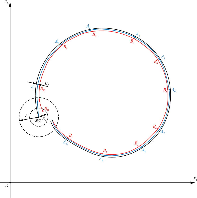
Figure 1: An example of illustration of the FGBFI-method on the plane. The points $A_{1},\ldots,A_{10}$ connect the parts of the approximate solution in forward time where the power series (6) are convergent, the points $B_{1},\ldots,B_{10}$ connect the parts for the backward time. The black line is projection of the trajectory arc of the system (5) (in general case) on the plane $x_{1}Ox_{2}$.

Next, we show the constructing algorithm of approximate solution:

1. Set the quantity $b_{m}$ of bits for the mantissa of a real number and accuracy $\varepsilon_{p}$ for the power series expansion. The number $b_{m}$ determines the machine epsilon $\varepsilon_{m}$. So we need to take with a reserve of this value, i.e. choose the value $b_{m}$, so that

   $$\varepsilon_{m}\ll\varepsilon_{p};$$

2. $t:=0$;

3. Set $X(0)\in B_{a}$ for the system (5), $way$ is direction in time (for going forward $way=1$, going backward $way=-1$), and $T$ (a length of the time segment);

4. $ended:=\mbox{{false}}$;

5. Calculate the integration step $\Delta t$ according to the formula (11) for $X(0)$;

6. If $\Delta t>T-t$ then $\Delta t:=T-t$, $t:=T$

   Else $t:=t+\Delta t$;

7. $\Delta t:=way\cdot\Delta t$;

8. Calculate the point $X(\Delta t)$ with the given accuracy $\varepsilon_{p}$ for the power series expansions;

9. Print$\big{(}way\cdot t,\>X(\Delta t)\big{)}$;

10. If $X(\Delta t)\notin B_{a}$ then Print(”Decrease the value $\varepsilon_{p}$ and/or $\varepsilon_{m}$”),

    $ended:=\mbox{{true}}$;

11. If $t=T$ then $ended:=\mbox{{true}}$;

12. If $ended$ then Finish the algorithm;

13. $X(0):=X(\Delta t)$;

14. Goto Step 5.

This algorithm can be applied to forward in time and backward too, making it a universal.

An example of illustration of the FGBFI-method on the plane is shown in Fig. 1. The points $A_{1},\ldots,A_{10}$ and $B_{1},\ldots,B_{10}$ are the projections on the plane $x_{1}Ox_{2}$ of the points $X(\Delta t)$ when running this algorithm. If a value of the accuracy $\varepsilon_{p}$ is large, then following in the backward time, we will go to infinity, because the solutions are strongly unstable at $t\rightarrow-\infty$. Therefore, the algorithm uses the ball $B_{a}$ for the control of finding approximate solutions within the boundaries of the attractor. For return to the given neighborhood $\varepsilon_{R}$, the value $\varepsilon_{p}$ (and the number $b_{m}$ respectively) selected in the calculating experiment. In fact, the value $\varepsilon_{R}$ determines how many digits of each coordinate of the point $B_{11}$ (see Fig. 1) must coincide with the digits of corresponding coordinates of the initial point $X(0)$ when we construct the approximate solution in the backward time. Also we use the configuration analysis of the approximate chaotic solution to check the accuracy it. In this case, we calculate the maximum degrees of piecewise polynomials which must be the same at the forward and backward time as in the articles [38, 39].

4  Calculating experiments

We made a calculating experiment for $N=5$, $H=3$ and $I=0.7$ [46] by the FGBFI-method. In the calculation, the point

$$x_{1}(0)=0.1450756817,\>\>x_{2}(0)=0.8395885828,\>\>x_{3}(0)=9.954786333$$

is found near the attractor. The calculation parameters are $b_{m}=160$, $\varepsilon_{m}=1.36846\cdot 10^{-48}$ and $\varepsilon_{p}=10^{-40}$. Following by the backward time, it is enough to get the coincidence of all the decimal places ($\varepsilon_{R}=10^{-10}$) of the initial conditions for computing in the time segment $[0,27.327]$. Also, the maximum degrees of piecewise polynomials coincide at the forward and backward time, i.e. the criteria of the article [39] for checking the accuracy of the approximate solution are performed.

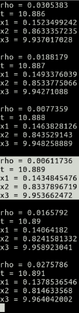
Figure 2: The screenshot of a computer program (for Linux) which outputs the distance $\rho$ and coordinates $x_{1}$, $x_{2}$ and $x_{3}$ of the trajectory point at time $t$ with the time step 0.001.

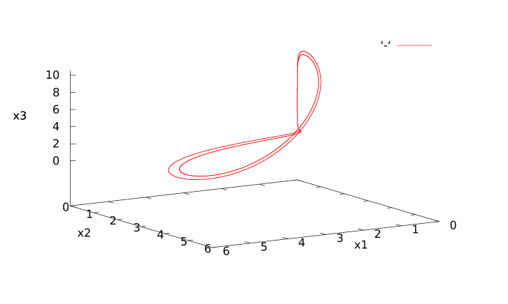
Figure 3: The trajectory arc constructed in the time segment $[0,27.327]$ for $N=5$, $H=3$ and $I=0.7$. $x_{1}(0)=0.1450756817$, $x_{2}(0)=0.8395885828$, $x_{3}(0)=9.954786333$.

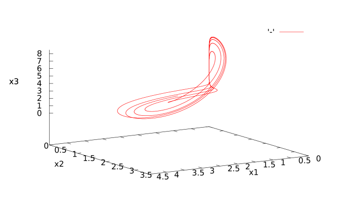
Figure 4: The trajectory arc constructed in the time segment $[0,30]$ for $N=5$, $H=3$ and $I=0.4$. $x_{1}(0)=1.292927957$, $x_{2}(0)=0.5183621413$, $x_{3}(0)=1.168939477$.

Table 1: The results of calculating experiment.

$n$	$t_{n}$	$x_{1}(t_{n})$	$x_{2}(t_{n})$	$x_{3}(t_{n})$	$\rho(t_{n})$
0	0	0.1450756817	0.8395885828	9.954786333	0
1	5.553	0.1201387594	0.7151506515	9.6198216985	0.358201
2	10.889	0.1434845476	0.8337896719	9.953662472	0.006117
3	16.439	0.1207485467	0.7178109534	9.6243463945	0.353004
4	21.778	0.1437352539	0.8342333601	9.9494643143	0.007668
5	27.327	0.118689978	0.7111230373	9.6323947777	0.348049

We recorded the rapprochements of trajectory with the initial point to the Table 1 (with the time step 0.001, see the highlighted strings in Fig. 2), wherein $t_{0}=0$,

$$\rho(t)=\sqrt{(x_{1}(t)-x_{1}(t_{0}))^{2}+(x_{2}(t)-x_{2}(t_{0}))^{2}+(x_{3}(t)-x_{3}(t_{0}))^{2}},$$

since the asymptotic trajectory is Poisson stable. Based on the observed values

$$\begin{array}[]{c}\rho(t_{0})\approx\rho(t_{2})\approx\rho(t_{4}),\>\rho(t_{1})\approx\rho(t_{3})\approx\rho(t_{5}),\\ t_{2}-t_{0}\approx t_{4}-t_{2}\approx t_{3}-t_{1}\approx t_{5}-t_{3}\approx 10.89,\end{array}$$

we have an approximation to the periodic solution with the period 10.89. However, the maximum Lyapunov exponent $\lambda_{\max}$ of this solution is positive and near to zero, and the Kaplan–Yorke dimension is near to integer value (see Table 5). Thus, for large values $t$, we leave the periodic regime (there is a weak chaotic solution). The trajectory arc constructed in the time segment $[0,27.327]$ is presented in Fig. 3.

The chaotic behaviour of the trajectories is observed $N=5$, $H=3$ and $I=0.4$ (see Fig. 4). Here, we also got the numerical solutions of the system (4) by the 4th order Runge–Kutta (RK4) method, researching the error $\varepsilon^{\{\mbox{\scriptsize rk4}\}}$ of this method for different steps $\Delta t^{\{\mbox{\scriptsize rk4}\}}$ (with a constant value) of integration,

$$\varepsilon^{\{\mbox{\scriptsize rk4}\}}=\sqrt{\left(x^{\{\mbox{\scriptsize rk4}\}}_{1}-x_{1}(T)\right)^{2}+\left(x^{\{\mbox{\scriptsize rk4}\}}_{2}-x_{2}(T)\right)^{2}+\left(x^{\{\mbox{\scriptsize rk4}\}}_{3}-x_{3}(T)\right)^{2}},$$

where $T=30$, $x^{\{\mbox{\scriptsize rk4}\}}_{1}$, $x^{\{\mbox{\scriptsize rk4}\}}_{2}$ and $x^{\{\mbox{\scriptsize rk4}\}}_{3}$ are the values of numerical solution by the RK4-method at $t=T$. The results are shown in Table 2. Since we are using the 10th characters after the decimal point as the accurate, then the error $3.68753\cdot 10^{-9}$ is not so great in relation to the length $T$ of the integration interval. Here, the maximum degree of the polynomials is equal to 25, the minimum degree is equal to 15 for the FGBFI-method.

Table 2: The error of the RK4-method compared with the FGBFI-method.

$\Delta t^{\{\mbox{\scriptsize rk4}\}}$	$\varepsilon^{\{\mbox{\scriptsize rk4}\}}$
0.05	0.0387658
0.01	$4.06488\cdot 10^{-5}$
0.005	$2.40695\cdot 10^{-6}$
0.001	$3.68753\cdot 10^{-9}$

Table 3: Comparison of the lengths $T$ of the integration intervals and accuracies $\varepsilon_{p}$ for different dynamic systems.

Dynamical system	$T$	$\varepsilon_{p}$
The Lorenz system [1, 37]	6.827	$10^{-50}$
The Chen system [16, 17, 38]	8.411	$10^{-53}$
The Sprott–Jafari system [39, 58]	34	$10^{-15}$
The system (4) [46]	30	$10^{-40}$

We compared the lengths $T$ of the integration intervals and accuracies $\varepsilon_{p}$ for different dynamic systems in Table 3. As this table shows, the value $\varepsilon_{p}$ is not so small for the Sprott–Jafari system [58]. This can be explained by the fact that the almost periodic solution (that we received in the article [39]) has very near to zero (or even negative) value $\lambda_{\max}$. Also note, $\lambda_{\max}$ for solution in Fig. 4 of the system (4) is positive and near to zero (see Sect. 5). Therefore, we have not such a big errors for the RK4-method.

5  Calculation of Lyapunov exponents

Usually, many researchers construct a linearized system of ODEs for the system (4) to determine the Lyapunov exponents. We propose to expand the system (4) by adding the linearized equations. The resulting system of 6th-order will also have a quadratic right-hand side. Let us show it.

Let $x_{4}(t)$, $x_{5}(t)$ and $x_{6}(t)$ are perturbations. We find (it is assumed that the vector $X$ is made up of three components)

$$\begin{array}[]{c}\dfrac{\partial\big{(}AX+\Phi(X)\big{)}}{\partial X}\left[\begin{array}[]{c}x_{4}\\ x_{5}\\ x_{6}\end{array}\right]=\vskip 6.0pt plus 2.0pt minus 2.0pt\\ =\left[\begin{array}[]{c}2Nx_{4}-2x_{1}x_{4}-Hx_{3}x_{4}-Hx_{1}x_{6}\vskip 6.0pt plus 2.0pt minus 2.0pt\\ x_{1}x_{4}+(4-I)x_{5}-0.28x_{2}x_{5}-0.5Hx_{3}x_{5}-0.5Hx_{2}x_{6}+0.002x_{3}x_{6}\vskip 6.0pt plus 2.0pt minus 2.0pt\\ 0.14x_{2}x_{5}+0.5Hx_{3}x_{5}-Ix_{6}+0.5Hx_{2}x_{6}-0.004x_{3}x_{6}\end{array}\right].\end{array}$$

Now we will work with the extended system (5). Then the matrix $A$ has the form

$$A=\left[\begin{array}[]{cccccc}2N&0&0&0&0&0\\ 0&4-I&0&0&0&0\\ 0&0&-I&0&0&0\\ 0&0&0&2N&0&0\\ 0&0&0&0&4-I&0\\ 0&0&0&0&0&-I\end{array}\right],$$

the matrices $Q_{1}$, $Q_{2}$ and $Q_{3}$ will contain zeros in new places,

$$Q_{4}=\left[\begin{array}[]{cccccc}0&0&0&-2&0&-H\\ 0&0&0&0&0&0\\ 0&0&0&-H&0&0\\ 0&0&0&0&0&0\\ 0&0&0&0&0&0\\ 0&0&0&0&0&0\end{array}\right],$$

$$Q_{5}=\left[\begin{array}[]{cccccc}0&0&0&1&0&0\\ 0&0&0&0&-0.28&-0.5H\\ 0&0&0&0&-0.5H&0.002\\ 0&0&0&0&0&0\\ 0&0&0&0&0&0\\ 0&0&0&0&0&0\end{array}\right],$$

$$Q_{6}=\left[\begin{array}[]{cccccc}0&0&0&0&0&0\\ 0&0&0&0&0.14&0.5H\\ 0&0&0&0&0.5H&-0.004\\ 0&0&0&0&0&0\\ 0&0&0&0&0&0\\ 0&0&0&0&0&0\end{array}\right],$$

$$\begin{array}[]{c}\|Q_{4}\|=\|Q_{4}\|_{1}=H+2,\vskip 6.0pt plus 2.0pt minus 2.0pt\\ \|Q_{5}\|=\|Q_{5}\|_{1}=\max\{0.5H+0.002,\>1\},\vskip 6.0pt plus 2.0pt minus 2.0pt\\ \|Q_{6}\|=\|Q_{6}\|_{1}=0.5H+0.14,\vskip 6.0pt plus 2.0pt minus 2.0pt\\ \displaystyle\mu=6\max_{p=\overline{1,6}}\|Q_{p}\|=6(H+2).\end{array}$$

Let

$$x_{4}(t)=\sum_{i=0}^{\infty}\alpha_{4,i}t^{i},\>\>\>x_{5}(t)=\sum_{i=0}^{\infty}\alpha_{5,i}t^{i},\>\>\>x_{6}(t)=\sum_{i=0}^{\infty}\alpha_{6,i}t^{i},$$

$$\begin{array}[]{c}\displaystyle r_{6,i}=\sum_{j=0}^{i}\alpha_{1,j}\alpha_{4,i-j},\>\>r_{7,i}=\sum_{j=0}^{i}\alpha_{3,j}\alpha_{4,i-j},\vskip 6.0pt plus 2.0pt minus 2.0pt\\ \displaystyle r_{8,i}=\sum_{j=0}^{i}\alpha_{1,j}\alpha_{6,i-j},\>\>r_{9,i}=\sum_{j=0}^{i}\alpha_{2,j}\alpha_{5,i-j},\vskip 6.0pt plus 2.0pt minus 2.0pt\\ \displaystyle r_{10,i}=\sum_{j=0}^{i}\alpha_{3,j}\alpha_{5,i-j},\>\>r_{11,i}=\sum_{j=0}^{i}\alpha_{2,j}\alpha_{6,i-j},\vskip 6.0pt plus 2.0pt minus 2.0pt\\ \displaystyle r_{12,i}=\sum_{j=0}^{i}\alpha_{3,j}\alpha_{6,i-j}.\end{array}$$

Then

$$\left\{\begin{array}[]{l}\alpha_{4,i+1}=\dfrac{2N\alpha_{4,i}-2r_{6,i}-Hr_{7,i}-Hr_{8,i}}{i+1},\vskip 6.0pt plus 2.0pt minus 2.0pt\\ \alpha_{5,i+1}=\dfrac{(4-I)\alpha_{5,i}+r_{6,i}-0.28r_{9,i}-0.5Hr_{10,i}-0.5Hr_{11,i}+0.002r_{12,i}}{i+1},\vskip 6.0pt plus 2.0pt minus 2.0pt\\ \alpha_{6,i+1}=\dfrac{-I\alpha_{6,i}+0.14r_{9,i}+0.5Hr_{10,i}+0.5Hr_{11,i}-0.004r_{12,i}}{i+1}.\end{array}\right.$$

We supplement the recurrence relations (10) by these relations.

We use the following modification of Benettin’s algorithm to determine the Lyapunov exponents:

1. Divide the segment $[0,T]$ by segments with length $\tau=T/M$, $M$ is the quantity that is given;

2. Let $Y^{(k)}=\left[\alpha_{1,0}^{(k)}\>\alpha_{2,0}^{(k)}\>\alpha_{3,0}^{(k)}\right]$, $Z^{(k)}_{(1)}=\left[\alpha_{4,0}^{(k,1)}\>\alpha_{5,0}^{(k,1)}\>\alpha_{6,0}^{(k,1)}\right]$, where $k=\overline{0,M}$. Similarly, Introduce two more vectors $Z^{(k)}_{(2)}$ and $Z^{(k)}_{(3)}$ similarly;

3. Input vector of the initial conditions $Y^{(0)}$ of researched solution for the system (4). Input $Z^{(0)}_{(1)}$, $Z^{(0)}_{(2)}$ and $Z^{(0)}_{(3)}\neq\textbf{0}$.

4. $k:=0$, $\lambda_{1}:=0$, $\lambda_{2}:=0$, $\lambda_{3}:=0$;

5. If $k\neq 0$ then $\lambda_{1}:=\lambda_{1}+\ln\left|Z^{(k)}_{(1)}\right|$, $\lambda_{2}:=\lambda_{2}+\ln\left|Z^{(k)}_{(2)}\right|$, $\lambda_{3}:=\lambda_{3}+\ln\left|Z^{(k)}_{(3)}\right|$;

6. Perform the normalization

   $$Z^{(k)}_{(1)}:=\dfrac{Z^{(k)}_{(1)}}{\left|Z^{(k)}_{(1)}\right|};$$

   Table 4: The groups of initial values $Z^{(0)}_{(m)}$ (before normalization) for the linearized system of ODEs.

   Group number	$Z^{(0)}_{(1)}$	$Z^{(0)}_{(2)}$	$Z^{(0)}_{(3)}$
   I	$\scriptsize\begin{array}[]{l}\alpha_{4,0}^{(0,1)}=5,\\ \alpha_{5,0}^{(0,1)}=7,\\ \alpha_{6,0}^{(0,1)}=13\end{array}$	$\scriptsize\begin{array}[]{l}\alpha_{4,0}^{(0,2)}=10,\\ \alpha_{5,0}^{(0,2)}=-1,\\ \alpha_{6,0}^{(0,2)}=11\end{array}$	$\scriptsize\begin{array}[]{l}\alpha_{4,0}^{(0,3)}=8,\\ \alpha_{5,0}^{(0,3)}=6,\\ \alpha_{6,0}^{(0,3)}=9\end{array}$
   II	$\scriptsize\begin{array}[]{l}\alpha_{4,0}^{(0,1)}=-6,\\ \alpha_{5,0}^{(0,1)}=13,\\ \alpha_{6,0}^{(0,1)}=5\end{array}$	$\scriptsize\begin{array}[]{l}\alpha_{4,0}^{(0,2)}=63,\\ \alpha_{5,0}^{(0,2)}=1,\\ \alpha_{6,0}^{(0,2)}=-17\end{array}$	$\scriptsize\begin{array}[]{l}\alpha_{4,0}^{(0,3)}=31,\\ \alpha_{5,0}^{(0,3)}=-7,\\ \alpha_{6,0}^{(0,3)}=19\end{array}$
   III	$\scriptsize\begin{array}[]{l}\alpha_{4,0}^{(0,1)}=1,\\ \alpha_{5,0}^{(0,1)}=-4,\\ \alpha_{6,0}^{(0,1)}=75\end{array}$	$\scriptsize\begin{array}[]{l}\alpha_{4,0}^{(0,2)}=7,\\ \alpha_{5,0}^{(0,2)}=-13,\\ \alpha_{6,0}^{(0,2)}=11\end{array}$	$\scriptsize\begin{array}[]{l}\alpha_{4,0}^{(0,3)}=-40,\\ \alpha_{5,0}^{(0,3)}=51,\\ \alpha_{6,0}^{(0,3)}=39\end{array}$
   IV	$\scriptsize\begin{array}[]{l}\alpha_{4,0}^{(0,1)}=1,\\ \alpha_{5,0}^{(0,1)}=1,\\ \alpha_{6,0}^{(0,1)}=2\end{array}$	$\scriptsize\begin{array}[]{l}\alpha_{4,0}^{(0,2)}=1,\\ \alpha_{5,0}^{(0,2)}=-37,\\ \alpha_{6,0}^{(0,2)}=11\end{array}$	$\scriptsize\begin{array}[]{l}\alpha_{4,0}^{(0,3)}=29,\\ \alpha_{5,0}^{(0,3)}=-3,\\ \alpha_{6,0}^{(0,3)}=5\end{array}$

   Table 5: The estimates of Lyapunov exponents and Kaplan–Yorke dimension for solution in Fig. 3.

   Group number	$\lambda_{1}$	$\lambda_{2}$	$\lambda_{3}$	$D_{KY}$
   I	0.0233993	0.0172255	$-2.15924$	2.0188
   II	0.0433011	0.00520866	$-2.16712$	2.0224
   III	0.0159841	$-0.0156199$	$-2.11898$	2.0233
   IV	0.018629	$-0.0180543$	$-2.11919$	2.0318

   Table 6: The estimates of Lyapunov exponents and Kaplan–Yorke dimension for solution in Fig. 4.

   Group number	$\lambda_{1}$	$\lambda_{2}$	$\lambda_{3}$	$D_{KY}$
   I	0.113902	$-0.726796$	$-1.82634$	1.1567
   II	0.104372	$-0.444632$	$-2.09897$	1.2347
   III	0.115022	$-0.472064$	$-2.08219$	1.2437
   IV	0.112198	$-0.454614$	$-2.09682$	1.2468

7. Calculate

   $$a^{(k)}:=\left\langle Z^{(k)}_{(2)},Z^{(k)}_{(1)}\right\rangle,\>Z^{(k)}_{(2)}:=Z^{(k)}_{(2)}-a^{(k)}Z^{(k)}_{(1)};$$

8. Perform the normalization

   $$Z^{(k)}_{(2)}:=\dfrac{Z^{(k)}_{(2)}}{\left|Z^{(k)}_{(2)}\right|};$$

9. Calculate

   $$\begin{array}[]{c}b^{(k)}:=\left\langle Z^{(k)}_{(3)},Z^{(k)}_{(1)}\right\rangle,\>c^{(k)}:=\left\langle Z^{(k)}_{(3)},Z^{(k)}_{(2)}\right\rangle,\vskip 6.0pt plus 2.0pt minus 2.0pt\\ Z^{(k)}_{(3)}:=Z^{(k)}_{(3)}-b^{(k)}Z^{(k)}_{(1)}-c^{(k)}Z^{(k)}_{(2)};\end{array}$$

10. Perform the normalization

    $$Z^{(k)}_{(3)}:=\dfrac{Z^{(k)}_{(3)}}{\left|Z^{(k)}_{(3)}\right|};$$

11. If $k\neq M$ then Build the three solutions of the extended system (5) in the time segment $[0,\tau]$ according to the algorithm in Sect. 3 with forward time. In this case, the initial conditions $X^{(k)}_{(1)}(0)$, $X^{(k)}_{(2)}(0)$ and $X^{(k)}_{(3)}(0)$ at $k$-th iteration for (5) formed as

    $$X^{(k)}_{(m)}(0)=\left[Y^{(k)}\>Z^{(k)}_{(m)}\right]^{\scriptsize\mbox{T}},\>m=\overline{1,3}.$$

    The first three components in the each obtained solution at $t=\tau$ $X^{(k)}_{(m)}(\tau)$ are the same. Record them in $Y^{(k+1)}$, the other components are recorded in $Z^{(k+1)}_{(m)}$ respectively;

12. $k:=k+1$;

13. If $k\leq M$ then Goto Step 5;

14. $$\lambda_{1}:=\dfrac{\lambda_{1}}{T},\>\lambda_{2}:=\dfrac{\lambda_{2}}{T},\>\lambda_{3}:=\dfrac{\lambda_{3}}{T};$$

15. Print($\lambda_{1}$, $\lambda_{2}$, $\lambda_{3}$).

We made the computational experiments for the four groups of vectors $Z^{(0)}_{(m)}$ (see Table 4). Their results are shown in Tables 5 and 6 ($D_{KY}$ is the Kaplan–Yorke dimension). The initial values of the vector components $Z^{(0)}_{(1)}$, $Z^{(0)}_{(2)}$ and $Z^{(0)}_{(3)}$ (before normalization) for the linearized system of ODEs are selected randomly. Also note, $M=20000$. Increasing $M$ does not affect the given values in Tables 5 and 6.

A feature of this modification of Benettin’s algorithm is to combine a linearized system of ODEs and the researched system (4) in the general form (5).

6  Acknowledgments

The reported study was funded by RFBR according to the research project 20-01-00347.

References

- [1] Lorenz, E.N. (1963), Deterministic nonperiodic flow, Journal of the Atmospheric Sciences, 20(2), 130-141.
- [2] Nemytskii, V.V. and Stepanov, V.V. (1989), Qualitative Theory of Differential Equations, Dover Publications: New York.
- [3] Guckenheimer, J. (1976), A Strange, Strange attractor, in the Hopf bifurcation and its application, Applied Mathematical Series, 19, 368-381.
- [4] Afraimovich, V.S., Bykov, V.V. and Shilnikov, L.P. (1977), The origin and structure of the Lorenz attractor, Soviet Physics Doklady, 22, 253-255.
- [5] Williams, R.F. (1979), The structure of Lorenz attractors, Publications mathématiques de l’IHÉS, 50, 321-347.
- [6] Kaplan, J.L. and Yorke, J.A. (1979), Preturbulence: a regime observed in a fluid flow model of Lorenz, Communications in Mathematical Physics, 6(2), 93-108.
- [7] Cook, A.E. and Roberts P.H. (1970), The Rikitake two-disc dynamo system, Mathematical Proceedings of the Cambridge Philosophical Society, 68(2), 547-569.
- [8] Tyson, J.J. (1977), On the appearance of chaos in a model of the Belousov reaction, Journal of Mathematical Biology, 5(4), 351-362.
- [9] Vallis, G.K. (1986), El Niño: A chaotic dynamical system? Science, 232(4747), 243-245.
- [10] Vallis, G.K. (1988), Conceptual models of El Niño and the Southern Oscillation, Journal of Geophysical Research, 93(C11), 13979-13991.
- [11] Sprott, J.C. (1994), Some simple chaotic flows, Physical Review E, 50(2), R647.
- [12] Sprott, J.C. (1997), Simplest dissipative chaotic flow, Physics Letters A, 228(4-5), 271-274.
- [13] Wei, Z. (2011), Dynamical behaviors of a chaotic system with no equilibria, Physics Letters A, 376(2), 102-108.
- [14] Wang, X., Chen, G. (2012), A chaotic system with only one stable equilibrium, Communications in Nonlinear Science and Numerical Simulation, 17(3), 1264-1272.
- [15] Stenflo, L. (1996), Generalized Lorenz equations for acoustic-gravity waves in the atmosphere, Physica Scripta, 53(1), 83-84.
- [16] Chen, G. and Ueta, T. (1999), Yet another chaotic attractor, International Journal of Bifurcation and Chaos, 9(7), 1465-1466.
- [17] Ueta, T. and Chen, G. (2000), Bifurcation analysis of Chen’s equation, International Journal of Bifurcation and Chaos, 10(8), 1917-1931.
- [18] Magnitskii, N.A. and Sidorov, S.V. (2006), New Methods for Chaotic Dynamics, World Scientific: Singapore.
- [19] Afraimovich, V., Gong, X. and Rabinovich, M. (2015), Sequential memory: binding dynamics, Chaos, 25, 103118.
- [20] Rabinovich, M.I., Afraimovich, V.S. and Varona, P. (2010), Heteroclinic binding, Dynamical Systems, 25(3), 433-442.
- [21] Dudkowski, D., Jafari, S., Kapitaniak, T., Kuznetsov, N.V., Leonov, G.A. and Prasad, A. (2016), Hidden attractors in dynamical systems, Physics Reports, 637(3), 1-50.
- [22] Yorke, J.A. and Yorke, E.D. (1979), Metastable chaos: the transition to sustained chaotic behavior in the Lorenz model, Journal of Statistical Physics, 21(3), 263-277.
- [23] Yao, L.-S. (2010), Computed chaos or numerical errors, Nonlinear Analysis: Modelling and Control, 15(1), 109-126.
- [24] Sparrow, C. (1982), The Lorenz Equations: Bifurcations, Chaos, and Strange Attractors, Springer: New York.
- [25] Kaloshin, D.A. (2001), Search for and stabilization of unstable saddle cycles in the Lorenz system, Differential Equations, 37(11), 1636-1639.
- [26] Sarra, S.A. and Meador, C. (2011), On the numerical solution of chaotic dynamical systems using extend precision floating point arithmetic and very high order numerical methods, Nonlinear Analysis: Modelling and Control, 16(3), 340-352.
- [27] Lorenz, E.N., Predictability: does the flap of a butterfly’s wings in Brazil set off a tornado in Texas? American Association for the Advancement of Science, 139th Meeting. AAAS Section on Environmental Sciences New Approaches to Global Weather: GARP (The Global Atmospheric Research Program), December 29, 1972.
- [28] Motsa, S.S. (2012), A new piecewise-quasilinearization method for solving chaotic systems of initial value problems, Central European Journal of Physics, 10(4), 936-946.
- [29] Motsa, S.S., Dlamini, P. and Khumalo, M. (2013), A new multistage spectral relaxation method for solving chaotic initial value systems, Nonlinear Dynamics, 72(1), 265-283.
- [30] Eftekhari, S.A. and Jafari, A.A. (2012), Numerical simulation of chaotic dynamical systems by the method of differential quadrature, Scientia Iranica B, 19(5), 1299-1315.
- [31] Chowdhury, M.S.H., Hashim, I. and Momani, S. (2009), The multistage homotopy-perturbation method: a powerful scheme for handling the Lorenz system, Chaos, Solitons and Fractals, 40(4), 1929-1937.
- [32] Gibbons, A. (1960), A program for the automatic integration of differential equations using the method of Taylor series, The Computer Journal, 3(2), 108-111.
- [33] Rall, L.B. (1981), Automatic Differentiation: Techniques and Applications, Springer-Verlag: Berlin – Heidelberg – New York.
- [34] Hashim, I., Noorani, M.S.M., Ahmad, R., Bakar, S.A., Ismail, E.S. and Zakaria, A.M. (2006), Accuracy of the Adomian decomposition method applied to the Lorenz system, Chaos, Solitons and Fractals, 28(5), 1149-1158.
- [35] Abdulaziz, O., Noor, N.F.M., Hashim, I. and Noorani, M.S.M. (2008), Further accuracy tests on Adomian decomposition method for chaotic systems, Chaos, Solitons and Fractals, 36(5), 1405-1411.
- [36] Al-Sawalha, M.M., Noorani, M.S.M. and Hashim, I. (2009), On accuracy of Adomian decomposition method for hyperchaotic Rössler system, Chaos, Solitons and Fractals, 40(4), 1801-1807.
- [37] Pchelintsev, A.N. (2014), Numerical and physical modeling of the dynamics of the Lorenz system, Numerical Analysis and Applications, 7(2), 159-167.
- [38] Lozi, R. and Pchelintsev, A.N. (2015), A new reliable numerical method for computing chaotic solutions of dynamical systems: the Chen attractor case, International Journal of Bifurcation and Chaos, 25(13), 1550187.
- [39] Lozi, R., Pogonin, V.A. and Pchelintsev, A.N. (2016), A new accurate numerical method of approximation of chaotic solutions of dynamical model equations with quadratic nonlinearities, Chaos, Solitons and Fractals, 91, 108-114.
- [40] Liao, S. (2009), On the reliability of computed chaotic solutions of non-linear differential equations, Tellus, 61A, 550-564.
- [41] Liao, S. (2013), On the numerical simulation of propagation of micro-level inherent uncertainty for chaotic dynamic systems, Chaos, Solitons and Fractals, 47, 1-12.
- [42] Liao, S. and Wang, P. (2014), On the mathematically reliable long-term simulation of chaotic solutions of Lorenz equation in the interval [0,10000], Science China – Physics, Mechanics & Astronomy, 57(2), 330-335.
- [43] Liao, S. (2014), Physical limit of prediction for chaotic motion of three-body problem, Communications in Nonlinear Science and Numerical Simulation, 19, 601-616.
- [44] Liao, S. and Li, X. (2015), On the inherent self-excited macroscopic randomness of chaotic three-body systems, International Journal of Bifurcation and Chaos, 29(5), 1530023.
- [45] Liao, S. (2017), On the clean numerical simulation (CNS) of chaotic dynamic systems, Journal of Hydrodynamics, 29(5), 729-747.
- [46] Llanos-Pérez, J.A., Betancourt-Mar, J.A., Cochob, G., Mansilla, R. and Nieto-Villar, J.M. (2016), Phase transitions in tumor growth: III vascular and metastasis behavior, Physica A: Statistical Mechanics and its Applications, 462, 560-568.
- [47] Arroyo, D., Hernandez, F. and Orúe, A.B. (2017), Cryptanalysis of a classical chaos-based cryptosystem with some quantum cryptography features, International Journal of Bifurcation and Chaos, 27(1), 1750004.
- [48] Luo, A.C.J. (2015), Periodic flows to chaos based on discrete implicit mappings of continuous nonlinear systems, International Journal of Bifurcation and Chaos, 25(3), 1550044.
- [49] Luo, A.C.J. (2015), Discretization and Implicit Mapping Dynamics, Springer: Heidelberg – New York – Dordrecht – London.
- [50] Wang, P., Liu, Y. and Li, J. (2014), Clean numerical simulation for some chaotic systems using the parallel multiple-precision Taylor scheme, Chinese Science Bulletin, 59(33), 4465-4472.
- [51] Mezzarobba, M. and Salvy, B. (2010), Effective bounds for P-recursive sequences, Journal of Symbolic Computation, 45(10), 1075-1096.
- [52] Chin, P.S.M. (1986), A general method to derive Lyapunov functions for non-linear systems, International Journal of Control, 44(2), 381-393.
- [53] Leonov, G.A. (2001), Bounds for attractors and the existence of homoclinic orbits in the Lorenz system, Journal of Applied Mathematics and Mechanics, 65(1), 19-32.
- [54] Zhang, F., Shu, Y. and Yang, H. (2011), Bounds for a new chaotic system and its application in chaos synchronization, Communications in Nonlinear Science and Numerical Simulation, 16(3), 1501-1508.
- [55] Li, D., Lu, J., Yu, X. and Chen, G. (2005), Estimating the bounds for the Lorenz family of chaotic systems, Chaos, Solitons and Fractals, 23(2), 529-534.
- [56] Wang, P., Li, D. and Hu, Q. (2010), Bounds of the hyper-chaotic Lorenz-Stenflo system, Communications in Nonlinear Science and Numerical Simulation, 15(9), 2514-2520.
- [57] Wang, P., Li, D., Wu, X., Lü, J. and Yu, X. (2011), Ultimate bound estimation of a class of high dimensional quadratic autonomous dynamical systems, International Journal of Bifurcation and Chaos, 21(9), 2679.
- [58] Jafari, S., Sprott, J.C. and Nazarimehr, F. (2015), Recent new examples of hidden attractors, The European Physical Journal Special Topics, 224(8), 1469-1476.