Efficient stream-based Max-Min diversification with minimal failure rate

Abstract

The stream-based Max-Min diversification problem concerns the task of selecting a limited number of diverse instances from a data stream. The nature of the problem demands immediate and irrevocable decisions. The set-wise diversity to be maximized is the minimum distance among any pair of the selected instances. Standard algorithmic approaches for sequential selection disregard the possibility of selection failures, which is the situation where the last instances of the stream are picked by default to prevent having an incomplete selection. This defect can be catastrophic for the Max-Min diversification objective. In this paper we present the Failure Rate Minimization (FRM) algorithm that allows the selection of a set of disparate instances while reducing significantly the probability of having failures. This is achieved by means of both analytical and empirical techniques. FRM is put in comparison with relevant algorithms from the literature through simulations on real datasets, where we demonstrate its efficiency and low time complexity.

I Introduction

Collecting and analyzing large amounts of data has become increasingly common and helpful for understanding complex systems. In some applications, data are presented to the system as a stream [20, 16] of sequentially arriving instances; for example, observations made by an autonomous robot while exploring an environment. Long or high-frequency data streams are difficult to handle by machines of limited computational and storage capacity. In addition, there is often a need for online processing that would output results as time goes, before the end of the stream. The online nature of the problem brings challenges to the static data preprocessing and mining methods. Most typically, this includes respecting time and memory limitations, the dynamic adaptation of learning algorithms, or dealing with non-stationarity where the properties of the incoming data change over time, e.g. due to phenomena such as concept drifting [17].

In this paper, we are interested in the online selection of a fixed and limited number of $b\in\mathbbm{N}^{*}$, called budget, such instances. Typically, less than 5% of the stream’s instances can be selected due to storage constraints. By definition, a selection from a stream is immediate and irrevocable since rejected instances cannot be called back, and discarding already selected instances might not be an option (e.g. materials or living samples may alter the local environment). Our attention is concentrated around the $b$-diversification problem [8, 1], also known as result diversification or $b$-dispersion problem, where a decision maker (DM) must select, out of a large pool of instances, a typically very small subset of them that are altogether as diverse as possible. Hence, the determined set contains a wide range of options, something particularly useful for instance when returning user query results or recommender systems [19, 23, 18, 21]. The diversity may represent dissimilarity, novelty, or semantic coverage of the instances, and there are several ways to quantify it for a set [9, 10].

Selecting diverse instances is therefore subject to a chosen evaluation criterion, i.e. a function to optimize throughout the process, hoping to be as good as possible at the end of it. In the Max-Sum diversification problem [6], the maximized evaluation criterion is the sum of the utility of the selected instances, while in the Max-Min diversification problem the DM wants to maximize the minimum distance between any two selected instances. Here, we choose to explore the latter as it is stricter and ensures that no two instances would be too ‘close’ if the selection strategy performs well. The notion of distance is inherent to a situation and assumed known in advance by the DM. This batch diversification problem has been proven NP-hard, however a few papers propose efficient approximation algorithms [12].

The stream-based version of the Max-Min diversification problem, formally introduced in [22], suits a wide range of real-life situations as they showed through various simulations on real datasets. More specifically, that work provided data from $d$-dimensional sequentially arriving insects or fishes, while an autonomus robotic device goes through a pre-defined path and decides immediately and irrevocably whether to select or not the current instance (i.e. insect or fish).

Motivation. A side effect of not being able to store the stream is suffering from frequent selection failures. This refers to the event of selecting by default the last incoming instances in order to prevent having an incomplete selection. Combined with the Max-Min objective function, this can significantly dramatically reduce the quality of the final selected set: in fact, it only requires one failure to deteriorate the entire quality of a set.

In this paper we address the stream-based Max-Min diversification problem by presenting the Failure Rate Minimization (FRM) algorithm that improves the quality of the selected set by significantly lowering the failure rate. Our simulations are based on datasets provided in [22]. That work proposed the DYN-SIMPLEK algorithm, which: first, during a mid-term analysis, finds a good approximation of the $b$-best selection set that an offline strategy would have selected, and then uses this knowledge for selecting from the instances that follow. Apparently, their preprocess on half of the data is a computationally heavy offline task that in many real-life situations is impractical. Instead, the proposed FRM algorithm is purely online and hence well-suited to selecting from streams with fast-incoming instances. More specifically, the FRM’s time complexity is $\mathcal{O}(Nd\log(N))$, which is at least $(N+b)/\log(N)$ times lower than that of the DYN-SIMPLEK. The FRM algorithm is put in comparison with relevant online algorithms from the literature through simulations where it shows its superior trade-off between time complexity and performance.

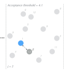
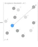
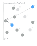
10pt 0pt 0pt 0pt 0pt 0pt 5pt 0pt 9pt 0pt 0pt 0pt 0pt 0pt 0pt 0pt

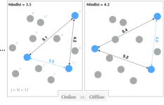
Figure 1: Example scheme of some steps of the irrevocable-choice $b$-diversification problem. Here $b=3$ instances must be selected out of $N=12$. The first instance $x_{1}$ ($j=1$) is accepted by default, then possible selections are decided immediately according to the instance score (inside the grey circle), i.e. their minimum distance w.r.t. to the already accepted instance ​​(s).

II The Max-Min diversification problem

II-A Translation to a score-based problem

Description. The Max-Min diversification problem is formalized as follows: a DM must select, out of a stream $\mathbf{X}\in^{d\times N}$ of $N\in\mathbbm{N}^{*}$ sequentially arriving instances, $b\in\mathbbm{N}^{*}$ of them (typically, $b\ll N$) so that the minimum distance between any two instances of this selected set $\dot{\mathbf{X}}_{b}\subseteq\mathbf{X}$ is maximized. Initially, the DM only knows the budget and the number of instances composing the stream.

We start by defining the minimum distance between every pair of instances that respectively belong to two sets $\mathbf{U}$ and $\mathbf{V}$ with:

$$D(\mathbf{U},\mathbf{V})=\min_{x_{i}\in\mathbf{U},\,x_{j}\in\mathbf{V}}\textup{Dist}(x_{i},x_{j}),$$ (1)

where $\textup{Dist}(x_{i},x_{j})\in_{+}$ is the distance between the instances $x_{i}$ and $x_{j}$. The notion of distance is given according to the nature of the data and the objective function; here this is computed with the Euclidean distance. When $\mathbf{U}=\mathbf{V}$, both instances belong to the same set and the minimum distance between every pair of instances is:

$$D(\mathbf{U})=\min_{x_{i},x_{j}\in\mathbf{U},\,i\neq j}\textup{Dist}(x_{i},x_{j}).$$ (2)

Then, expressing the above for any selection set $D(\dot{\mathbf{X}}_{b})$, allows us to formally define the $b$-size best selection set:

$$\dot{\mathbf{X}}_{b}^{*}=\operatorname*{\arg\!\max}_{\dot{\mathbf{X}}_{b}\subseteq\mathbf{X},|{\dot{\mathbf{X}}_{b}}|=b}\,\,D(\dot{\mathbf{X}}_{b}),$$ (3)

and the maximum distance associated to this set becomes $D^{*}=D(\dot{\mathbf{X}}_{b}^{*})$.

Mapping to a score-based sequential selection problem. To investigate online selection from a stream involves translating this type of process into a more generic problem of sequential selection that is easier to handle, and for which we can apply algorithms that are commonly used in the literature, such as the standard Secretary Problem algorithms [14, 11]. The idea is to associate each instance to a score that represents its worth for the DM, i.e. how valuable the instance is for the selection.

More formally, the scoring function $s:^{d}\rightarrow_{+}$ maps an instance into a real-valued score. By that, the DM is allowed to use any score-based or rank-based sequential selection method. However, in the large majority of cases, the score distribution is unknown a priori and is likely to change depending on the choice of scoring function. In this particular case, there is no ‘correct way’ to compute a score for an instance, since, as stated earlier, the $b$-diversification problem is NP-hard even in the offline case. In other words, there is no unique score that reflects the inherent value of an instance.

The goal here is therefore to propose a step-wise scoring function that is appropriate to every instance, while depending on the process’ step. The score of the instance arriving at step $j$, $S_{j,k}\in_{+}$, should depend on the $k\leq b$ instances selected so far, written as $\dot{\mathbf{X}}_{k}=\{\dot{x}_{1},...,\dot{x}_{k}\}\subseteq\mathbf{X}$, at positions $\{m_{1},...,m_{k}\}$ of the sequence (hence, $\dot{x}_{l}=x_{m_{l}},\,\forall l\leq k$). We propose the following score for the $j$-th arriving instance:

$$S_{j,k}=D\left(\dot{\mathbf{X}}_{k},\,\{x_{j}\}\right)\,\,\in_{+},\,\,\forall j\leq N,\,\,\forall k\leq b,$$ (4)

which merely computes the minimum distance between this instance and every previously selected instances.

Remark 1

When the data distribution is unknown, it is meaningless to assign a score to an instance when none has been selected yet. Therefore we assume that, regardless the strategy used, the first incoming instance is always selected, i.e. $m_{1}=1$. This same assumption was considered in [22] (see Sec. 4.1.1 therein) and their conducted empirical study concludes that, as long as $b$ is reasonably large, the first instance selected has a marginal effect on the overall quality of the selection when using their algorithm, which is also verified with our algorithm proposed in Sec. III.

Then, in order to avoid null scores when $k>1$, we propose the following to define the score of the $l$-th already selected instance at any time:

$$\!\!\!\dot{S}_{m_{l},k}=D\left(\dot{\mathbf{X}}_{k}\backslash x_{m_{l}},\,\{x_{m_{l}}\}\right)\in_{+},\,\,\forall l\leq k,\,\forall k\leq b.\!\!\!\!\!\!\!$$ (5)

This computes the minimum distance between this instance and every other previously selected instances.

The sequence of decisions $\mathbf{A}=(A_{j})_{j\geq 1}$ regarding the instances is such that $A_{j}=1$ if the $j$-th instance is accepted and 0 otherwise, in particular $A_{m_{1}}=...=A_{m_{k}}=1$. An algorithm’s performance is given through the following criterion, called the reward, evaluated at the end of the process and defined as $\mathbbm{E}[\phi(\mathbf{S},\mathbf{A})]$, where:

$$\phi(\mathbf{S},\mathbf{A})=\!\!\!\min_{1\leq j\leq N}(S_{j,b}\,\,A_{j})=\!\!\!\min_{1\leq l\leq b}\dot{S}_{m_{l},b}:=D(\dot{\mathbf{X}}_{b})\,\,\in_{+},$$ (6)

with $\mathbf{S}=(S_{j,b})_{j\leq N}$ the vector of instances scores at the end of the selection. The DM’s goal is therefore to maximize the $\mathbbm{E}[\phi(\mathbf{S},\mathbf{A})]$.

Example. The scheme of an example is shown in Fig. 1, where the DM has to select $b=3$ instances out of $N=12$ sequentially incoming instances. Say that the very first instance is selected, i.e. $m_{1}=1$. The score of the $j$-th arriving instance is the distance between that and the initially selected instance $x_{1}$. The algorithm selects the $j=8$-th instance since its distance to $x_{1}$ is greater than the acceptance threshold, i.e. $\textup{Dist}(x_{1},x_{8})=4.8>4.1$. This selection leads to a relaxation in the acceptance threshold for the next step ($j=9$). The last instance selected is the $j=11$-th one. At the end, the selected instances are $m_{1}=1$, $m_{2}=8$ and $m_{3}=11$, which gives a final reward of $\phi=\min(3.5,3.5,4.2)=3.5$. This can be put in comparison with the reward of an offline strategy (it has access to the batch of all instances from the beginning) that is worth $\phi_{\textup{off}}=4.2$ in this example.

II-B Failures

The irrevocable aspect of every stream-based selection problem implies a possible selection by default near the end of the sequence in order to fill the budget, called failure, see definition below.

Definition 1

Failure and failure rate ($f_{j}$): A failure at step $j$, when $k$ instances have been selected already, is the event of accepting a last incoming instance by default to fill any empty slots:

$$f_{j}=\mathds{1}\{N-j+1=b-k\}.$$ (7)

This measure is computed at every test, such that the failure rate is $\rho_{f}=\frac{1}{T}\sum_{\textup{test}=1}^{T}\mathds{1}\{f_{j}(\textup{test})>0\}$, where $T$ is the total number of tests. Therefore, it defines the frequency at which an algorithm fails at selecting an instance before the end of the stream, and thus should be kept as low as possible.

Selection failures are clearly undesirable, especially in the $b$-diversification problem for which a selection by default is very likely to lower the overall quality of the selection set, since an instance selected by failure might be arbitrary close to a previously selected instance.

III The Failure Rate Minimization

III-A Principle

The central idea of the Failure Rate Minimization (FRM) algorithm is to improve the reward by significantly lower the aforementioned failure rate. Firstly, it splits the stream into $b$ subsequences (or rounds) of size $n=\lfloor N/b\rfloor$, then aiming to select exactly one instance from each of them. In fact, working with one selection per round allows the derivation of a few analytical results, whereas finding closed-form results become necessarily more complex when handling the selection of $b$ instances altogether. For simplicity, we focus on a single round in this section (see Alg. 1 for the deployment of one round), therefore we omit the subscript $k$ that refers to the current round. Recall that the first selected instance has no impact on the quality of the final selection, therefore the selection from the first subsequence is arbitrary, hence we set $m_{1}=1$.

Each subsequence is further divided in two phases: the learning phase of size $c\in\mathbbm{N}^{*}$ (also called cutoff) (see lines 1-3 in Alg. 1) where all instances are systematically rejected, followed by the selection phase (see lines 4-16 in Alg. 1). This is similar to the standard Secretary Problem algorithm [11]. In the former, the DM records the best instance, here the farthest away from the first selected instance, which dictates the acceptance threshold $\tau\in_{+}$ for the next instances in the subsequence (see line 3 in Alg. 1). The process terminates when an instance is selected, i.e. when $S_{j}>\tau,\,\forall j\in\{c+1,...,n\}$, or at the end of the subsequence if none managed to beat the acceptance threshold, i.e. in case of a failure. If the latter occurs, the last instance of the subsequence is selected by default.

The optimal size of the learning phase is subject to a close investigation as it evolves according to the DM’s objective function. In the well-known algorithm proposed in [11], it is set to $c=\lfloor n/e\rfloor$. This is shown to be optimal when the DM’s goal is to maximize the probability of selecting the best instance, and when $n$ goes to infinity while the ratio $c/n$ remains constant. However, when instances have underlying scores and the objective is to maximize the score of the selected instance, then the optimal size becomes $c=\sqrt{n}-1$ [5], provided that the underlying score distribution is uniform on $[0,1]$. Since our objective is closer to the second option, we use $c=\sqrt{n}-1$ in the rest of the paper.

III-B The low-failures adjustment

Our idea to mitigate the effects of failures is to define a switch $j^{*}\in\{1,...,N\}$, i.e. an index into the subsequence at which the acceptance threshold turns from static to dynamic. Two questions naturally arise:

• How to choose an appropriate switch value $j^{*}$?

• How to dynamically adjust the threshold for $j>j^{*}$?

The first interrogation is answered analytically, while the second results from an empirical study.

Definition 2

Switch ($j^{*}$): Index into the instance sequence for which the acceptance threshold $\tau_{j}$ becomes dynamic:

$${\tau}_{j}:=\begin{cases}\tau&j<j^{*},\\ \tau^{\textup{upd}}_{j}&\textup{otherwise},\\ \end{cases}$$ (8)

where $\tau^{\textup{upd}}_{j}$ is the updated acceptance threshold from $j^{*}$ and on, and is the subject of the second point.

(Q1) We start by addressing the first point by computing the expected stopping time assuming that no failure occurred and that the horizon is finite. Since selecting an instance means putting an end to the subsequence, we start by investigating the expectation of the decision variable $\tilde{A}_{j}:=\sum_{i=c+1}^{j}A_{i}\in\{0,1\}$. More specifically, we compute its expectation given that there were no failure; formally it is written: ${\mu}_{j}(c):=\mathbbm{E}[\tilde{A}_{j}\mid\textup{no fail.}],\,\ \forall j$, see Proposition 2.

Proposition 1

Set a pool of $n\in\mathbbm{N}$ totally ordered instances, i.e. each of them having a rank from 1 (the best) to $n$ (the worst). The expectation $\gamma(b,c)\in\{1,...,n\}$ of the absolute rank of the $b$-th best instance out of a subset of $c\in\mathbbm{N}$ of them is given by:

$$\gamma(b,c)=\frac{b(n+b)}{c+b}.$$ (9)

Proof:

The proof uses backward induction, i.e. we first consider the case where $c=n$. Since every instance has been rejected, we have $\gamma(c=n)=b$. Let us go one step ahead and consider the case where $c=n-1$, which implies that $\gamma=b$ if the instance that has not been examined is not among the absolute $b$-best, and $b+1$ if it is. Hence, $\gamma(c=n-1)=b\frac{c}{b+c}+(b+1)\frac{b}{b+c}$. By recursion, we get:

$$\gamma(c) =\sum_{m=0}^{n-c}\binom{n-c}{m}\left(\frac{c}{b+c}\right)^{n-c-m}\left(\frac{b}{b+c}\right)^{m}(b+m),$$

$$\Leftrightarrow\ \ \gamma(c) =\frac{b(n+b)}{b+c}.$$

Setting $b=1$ leads to Proposition 9. ∎

Proposition 2

The expectation $\mu_{j}$ and the standard deviation $\sigma_{j}$ of the number of instances accepted at step $j$ given that there is no failure in the end is given by:

$${\mu}_{j}(c) =\displaystyle\frac{1-(1-\frac{\gamma-1}{n})^{j-c}}{1-(1-\frac{\gamma-1}{n})^{n-c}},$$ (10)

$$\sigma_{j}(c) =\sqrt{{\mu}_{j}(c)-{{\mu}_{j}(c)}^{2}};$$ (11)

where $\gamma=\gamma(1,c)$ is given in Proposition 9.

Proof:

The ‘no failure’ event happens with probability $1-\mathbbm{P}(\tilde{A}_{n}=0)$ and hence, the expected number of selected instances given that there were no failure is given by $\mathbbm{E}[\tilde{A}_{j}|\textup{no fail.}]={\mathbbm{P}(\tilde{A}_{j}=1,\,\tilde{A}_{n}=1)}/{\mathbbm{P}(\text{no fail.})}$. Hence:

$$\mathbbm{E}[\tilde{A}_{j}|\textup{no fail.}]=\frac{\mathbbm{P}(\tilde{A}_{j}=1)}{1-\mathbbm{P}(\tilde{A}_{n}=0)} =\frac{1-\prod_{i=c+1}^{j}\mathbbm{P}(X_{i}\geq\gamma)}{1-\prod_{j=c+1}^{n}\mathbbm{P}(X_{j}\geq\gamma)},$$

$$\Leftrightarrow\,\,\mathbbm{E}[\tilde{A}_{j}|\textup{no fail.}] =\frac{1-\left(1-\frac{\gamma-1}{n}\right)^{j-c}}{1-\left(1-\frac{\gamma-1}{n}\right)^{n-c}}.$$

The formula for the variance is obtained using the fact that $\mathbbm{E}[(\tilde{A}_{j})^{2}|\textup{no fail.}]=\mathbbm{E}[\tilde{A}_{j}|\textup{no fail.}]$. ∎

We use Proposition 2 to compute ${\mu}_{j}:={\mu}_{j}(c=\sqrt{n}-1),\,\ \forall j\in\{1,...,n\}$. To avoid failure from happening, a natural option is to compare the current number of selections with its expected mean, and therefore we set the following rule: if $\tilde{A}_{j}$ is more than $\sigma_{j}$-away from its expected mean, the threshold should be relaxed. Here, $\tilde{A}_{j}$ is always equal to zero (when an instance is selected, the subsequence ends), the previous condition therefore results in switching from a static to a dynamic threshold whenever $0\leq{\mu}_{j}-{\sigma}_{j}$. Consequently, ${\mu}_{j^{*}}=\sigma_{j^{*}}$, and using Eq. 11 we get $j^{*}$ by solving $\mu_{j^{*}}=1/2$.

(Q2) We now address the second point. After the switch, the threshold gets relaxed by tracking the value of $\tau$ in the list of scores seen so far in the subsequence, and from that is lowered by $q_{j}$ positions until the process ends (see lines 7-9 in Alg. 1). Formally, we write $\tau^{\textup{upd}}_{j}=S^{\textup{ord}}_{p+q_{j},j}$ where $(S^{\textup{ord}}_{1,j},...,S^{\textup{ord}}_{j,j})$ is the ordered sequence of scores up to the $j$-th instance, i.e. $S^{\textup{ord}}_{1,j}>...>S^{\textup{ord}}_{j,j}$, and $p$ is the position in the ordered sequence at which $S^{\textup{ord}}_{p,j}=\tau$. The decremental function $q_{j}$ defines how the threshold gets relaxed according to $j$ (for instance lower the score by one position every step, two steps, three steps etc.) and is tuned empirically, as shown in the simulation section.

III-C Time complexity

At every round of the FRM algorithm, the entire learning phase requires $\mathcal{O}(c\log(c)d)$ time, i.e. $\mathcal{O}\left(\sqrt{n}\log({\sqrt{n}})d\right)$ operations, as it only sorts the $c=\lfloor\sqrt{n}\rfloor$ first instances. It takes $\mathcal{O}((n-c)d)$, i.e. $\mathcal{O}((n-\sqrt{n})d)$ time to go through the selection phase, i.e. to compare each $d$-dimensional instance to a fixed scalar score, without any adaptation from the DM. Replacing a fixed acceptance threshold with a dynamic one requires to compare every new instance with the sorted vector of already seen scores, hence it needs $\mathcal{O}((n-c)d\log(n))$, i.e. $\mathcal{O}((n-\sqrt{n})d\log(n))$ operations. The entire time complexity of the FRM algorithm is therefore $\mathcal{O}((N-\sqrt{Nb}/2)d\log(N/b))$, or more simply $\mathcal{O}(Nd\log(N))$. Note that this is significantly lower than the $\mathcal{O}(N^{2}(d+1)+Nd(b+1))$ complexity of the DYN-SIMPLEK algorithm built for the $b$-diversification problem [22] (see Sec. IV-A for details).

Algorithm 1 One round of the FRM algorithm

Input: the scores of the sequentially incoming instances $(S_{1},...,S_{n})$, the cutoff value $c$ and the decremental function $q_{j},\,\,\forall j\leq n$.

Output: the final decision vector $\mathbf{A}$

1:  

2:​​​​​​​​_■ Learning phase

3:  

4:$\mathbf{A}_{1,...,c}\leftarrow 0$/​/ reject by default all $c$ first instances

5:$\mathbf{S}^{\textup{ord}}_{c}\leftarrow\text{sort}(S_{1},...,S_{c})$

6:$\tau\leftarrow S^{\textup{ord}}_{1,c}$

7:  

8:​​​​​​​​_■ Selection phase

9:  

10:for $j=c+1$ to $n$ do

11:    if  $0<{\mu}_{j}-{\sigma}_{j}$ then /​/ set the acceptance threshold

12:        $\tau_{j}=\tau$

13:    else

14:        $p\leftarrow\textup{find\_index}(\mathbf{S}^{\textup{ord}}_{j}=\tau)$

15:        $\tau_{j}=S^{\textup{ord}}_{p+q_{j},j}$

16:    end if

17:    if $S_{j}>\tau_{j}$ or   $j=n$ then /​/ compare to threshold or failure

18:        $A_{j}\leftarrow 1$

19:    else

20:        $A_{j}\leftarrow 0$

21:    end if

22:end for

IV Simulations

IV-A Relevant algorithms from the literature

In an effort to compare our algorithm with those already proposed in the sequential selection literature, we first give brief explanations for each of them. Note that, instances are assumed to arrive uniformly at random.

KLEINBERG (2005) – The algorithm presented in [13], called KLEINBERG here for simplicity, proceeds as follows: the DM draws a random value $m\sim\text{Binom}(N,1/2)$ and recursively apply the standard secretary problem algorithm (see [11]) to select up to $l=\lfloor b/2\rfloor$ instances among the first $m$ instances. After the $m$-th instance, it selects every instance that exceeds the $l$-th best seen during the first phase, (i.e. $\tau_{j}=S^{\textup{ord}}_{l,m}\,\,,\,\,\forall j>m$) until every empty slot is filled.

OPTIMISTIC (2007) – The OPTIMISTIC algorithm [3] separates the entire sequence into a learning phase of size $c=\lfloor N/e\rfloor$, and a selection phase. The acceptance threshold $\tau_{j}$ is dynamic and is equal to the relative rank of the $b$-th best recorded during the learning phase when no instance has been accepted yet, i.e. $\tau_{j}=S^{\textup{ord}}_{b,c}$  for  $\sum_{i=c+1}^{j}A_{i}=0$, the $b-1$-th best when one instance has been accepted, i.e. $\tau_{j}=S^{\textup{ord}}_{b-1,c}$  for  $\sum_{i=c+1}^{j}A_{i}=1$, etc. up to the last instance accepted. Note that when $b=1$ it degenerates to the standard algorithm proposed in [11].

Hiring-above-the-mean (MEAN) (2009) – The MEAN [7] algorithm’s acceptance threshold is the average score of the instances selected so far; it adapts to each new selection.

SUBMODULAR (2013) – The work of [4] studies a general setting where the objective function is submodular, i.e. the benefit of each instance’s selection is non-increasing as the set grows. Similar to the FRM algorithm, the entire stream is divided into $b$ subsequences. In each of them, the standard secretary problem is applied, i.e. $c=\lfloor N/(be)\rfloor$ instances are rejected by default at the beginning of each subsequence, and exactly (respectively at most) one instance is accepted in [15] (respectively [4]) in every of them.

DYN-SIMPLEK (2016) – The so-called SIMPLEK algorithm [22] operates as follows: the DM systematically rejects by default the first $c=\lfloor N/2\rfloor$ instances and from them computes an acceptance threshold for the instances that will follow using binary search. According to the authors, this step takes $\mathcal{O}(cd)$ to store the $c$ instances, then $\mathcal{O}(N^{2}d)$ time to compute the threshold (see Sec. 5.1 therein). Here we denote this threshold by $\gamma_{\textup{off}}\in_{+}$ since it requires a rather costly offline computation to have been made. In the selection phase that follows, the first arriving instance is always selected, i.e. $m_{1}=\lfloor N/2\rfloor+1$. Next, every instance whose distance to the latter is greater or equal to the acceptance threshold $\gamma_{\textup{off}}$ gets selected until $b$ instances are selected.

In order to avoid a high failure rate, which is approximately $\rho_{f}=35\%$ using this static acceptance threshold (see Sec 4.2.1 in the original paper), the authors propose the DYN-SIMPLEK. The dynamic threshold $\gamma_{j}$ at the current step $j$ is set such that the area below the pdf curve between that and to the right is ${(b-k)}/{(N-j)}$, where $k$ is the number of instances selected so far. Finally, the new acceptance threshold is set to the minimum between that and $\gamma_{\textup{off}}$ at each step $j$. This manipulation allows to significantly reduce the failure rate, as shown in the next simulations. In the selection phase, the time complexity is $\mathcal{O}(Nd)$ for every selection, i.e. $\mathcal{O}(Ndb)$ in total, and $\mathcal{O}(N)$ for every other rejected instance, i.e. $\mathcal{O}((N-N/2-b)N)$ overall. Finally, the entire algorithm time complexity is $\mathcal{O}(N^{2}(d+1/2)+(d/2+bd-b)N)$.

SINGLE-REF (2019) – The SINGLE-REF algorithm [2] also separates the entire stream in two phases, and takes as input a cutoff $c$ and a fixed acceptance threshold $\tau_{j}$, both empirically optimized according to the budget $b$. For instance, when $b=5$, $c=0.2525\,N$ and $\tau_{j}=S^{\textup{ord}}_{2,c}$, i.e. each candidate should beat the second best recorded during the learning phase, and when $b=50$, $c=0.1536\,\,N$, $\tau_{j}=S^{\textup{ord}}_{9,c}$. A wide table of these optimized parameters is provided in the paper.

IV-B Set-up

Inspired by the simulations of [22], we start with data from $N=5000$ $z$-normalized synthetic random walks. The walks are reshuffled to produce $100$ streams of $N$ walks of the original dataset ordered randomly.

In Fig. 2 is displayed the minimum distance between the set of $b=10$ selected instances using the different strategies described in the previous subsection, averaged over the $100$ tests. The red line represents the median performance of each strategy, the blue box the quantiles, the whiskers extend to the most extreme data points not considered outliers, and finally the outliers are plotted individually with red dots.

Fig. 3(a) (resp. Fig. 3(b)) displays the minimum distance between the set of $b=8$ (resp. $b=4$) selected instances of dimension $d=256$ (resp. $d=463$) out of a stream of $N=1200$ insects (resp. $N=200$ fishes), using the same strategies as in Fig. 2, averaged over $500$ tests, this time using the real data provided again in [22].

IV-C Empirical tuning of FRM

The parameter of FRM that stipulates how the threshold is relaxed after the switch, we start by using a simple function that decreases the threshold by one position at a time, namely $q_{j}=1,\ \forall j\in\{1,...,n\}$. Having a constant decrement might not be the best option because it does not quantify how many instances are left and might lead to an algorithm that is not competitive enough. Another option is to change for an exponential decrement $q_{j}=\lfloor e^{(j-v_{1})/v_{2}}\rfloor$, with $v_{1}$ and $v_{2}$ empirically computed constants. Simulations on synthetic data show that using $q_{j}=1$ leads to a median of $D=23.62$ and $\rho_{f}=0\%$, whereas setting $q_{j}=\lfloor e^{(j-v_{1})/v_{2}}\rfloor$ with the empirically optimized parameters $v_{1}=412$ and $v_{2}=72$, leads to a median of $D=26.67$ while maintaining a zero failure rate ($\rho_{f}=0.0\%$), hence it is the one used in the following simulations.

0pt 0.45pt 0pt 0pt

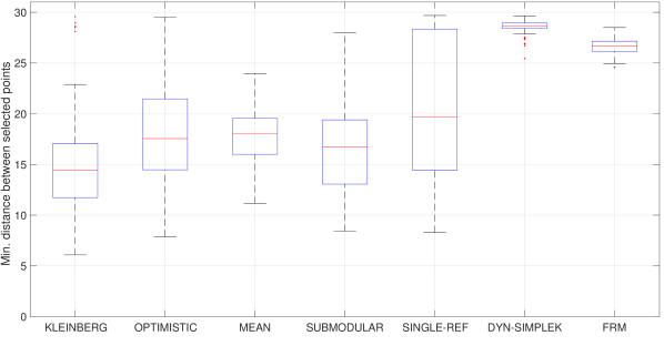
Figure 2: Minimum distance between the $b=10$ selected instances on synthetic random walks producing streams of length $N=5000$.

0pt 0.45pt 0pt 0pt

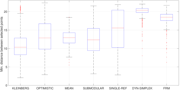
(a) Data from a sequence of $N=1200$ insects with $b=8$ slots.

0pt 0.45pt 0pt 0pt

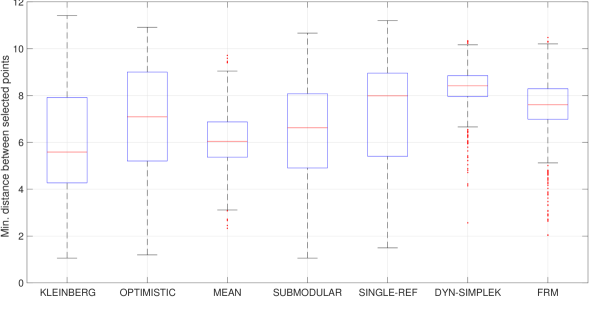
(b) Data from a sequence of $N=200$ fishes with $b=4$ slots.

Figure 3: Minimum distance between the selected instances in two scenarios considered for real data provided in [22], containing samples collected by an autonomous robot that are either insects or fishes.

IV-D Simulations results

IV-D1 Synthetic data

A striking result from the simulations on synthetic random walks concerns their associated failure rates, shown in the RW column of Tab. I. As the ratio between the budget of instances to select and the length of the stream is rather short ($b/N=2.10^{-3})$, the chances that the algorithm will fail to fill all $b=10$ empty slots should be, intuitively, quite low. The failure rates for the KLEINBERG, OPTIMISTIC, and SUBMODULAR strategies are however surprisingly high (all close to 100%), and lead to a poor quality of the resulting selected sets. More specifically, they achieve a median of approximately $D\approx 17$, when the median of a strategy with a slightly better failure rate of $63\%$ (see SINGLE-REF in Tab. I) already climbs to $D\approx 20$ (see SINGLE-REF in Fig. 2).

A second observation concerns the MEAN strategy, which always has the lowest failure rate (see MEAN in Tab. I), yet does not manage to output a high-quality selection set (the median is at $D\approx 17$). This is due to the algorithm procedure: $x_{1}$ is selected, $x_{2}$ is rejected and the score of $x_{1}$ becomes its distance to $x_{2}$. Then, subsequent instances are selected if their score is higher than that of $x_{1}$, hence the acceptance threshold is initially rather low and the algorithm is not competitive.

Finally, observe that the FRM’s performance is very close to that of the DYN-SIMPLEK algorithm, and in addition lowers the upper bound for the time complexity by a factor of at least $(N+b)/\log(N)$. It presents small differences in the quantiles, i.e. a narrow blue box, and by that constitues the most reliable option among the proposed purely online strategies.

IV-D2 Real dataset

Unsurprisingly, the results on real-data portrayed in Fig. 3 comply with those previously seen on synthetic random walks. FRM remains the algorithm with the best trade-off between time complexity and performance by maintaining a low failure rate. Moreover, the difference in achievement gets smaller as the number of instances to select from declines.

	Datasets
Online strategy	RW	Insects	Fishes
	$\rho_{f}$   $D$	$\rho_{f}$   $D$	$\rho_{f}$   $D$
KLEINBERG	94.0  14.4	92.4  10.3	73.8  5.8
OPTIMISTIC	87.0  17.5	83.4  12.7	59.8  7.1
MEAN	0.0  17.9	0.0  12.8	1.0  6.0
SUBMODULAR	100.0  17.3	96.2  12.5	77.8  6.7
SINGLE-REF	63.0  19.8	56.2  15.5	48.4  8.0
FRM (proposed)	0.0  26.7	4.8  18.5	5.7  7.5

TABLE I: Table of the combinations between failure rate $\rho_{f}$ in % and median minimum distance $D$ for different online strategies (rows) and different datasets (columns).

V Conclusion and discussion

This paper investigated the stream-based Max-Min $b$-diversification problem in which the decision maker’s goal is to select the most diverse set possible out of the instances of a data stream. We propose to translate the setting to a score-based sequential selection problem, for which we can apply already existing algorithms from the literature. The FRM algorithm presented in this paper is based on reducing the selection failures that naturally occur in this setting: it is easy-to-implement, efficient and fast in practice. More specifically, the FRM’s time complexity is $\mathcal{O}(Nd\log(N))$, i.e. at least $(N+b)/\log(N)$ times lower than that of the DYN-SIMPLEK algorithm that serves as performance target. Finally, the performance of FRM is compared to relevant existing online algorithms through simulations on real datasets.

References

- [1] T. Akagi, T. Araki, T. Horiyama, S.-i. Nakano, Y. Okamoto, Y. Otachi, T. Saitoh, R. Uehara, T. Uno, and K. Wasa, “Exact algorithms for the Max-Min dispersion problem,” in Frontiers in Algorithmics, J. Chen and P. Lu, Eds., 2018.
- [2] S. Albers and L. Ladewig, “New results for the -secretary problem,” in International Symposium on Algorithms and Computation (ISAAC), ser. Leibniz International Proceedings in Informatics (LIPIcs), vol. 149, 2019, pp. 18:1–18:19.
- [3] M. Babaioff, N. Immorlica, D. Kempe, and R. Kleinberg, “A knapsack secretary problem with applications,” in APPROX-RANDOM, 2007.
- [4] M. Bateni, M. Hajiahghayi, and M. Zadimoghaddam, “Submodular secretary problem and extensions,” in ACM Transactions on Algorithms, vol. 9, 2013, pp. 39–52.
- [5] J. Bearden, “A new secretary problem with rank-based selection and cardinal payoffs,” in Journal of Mathematical Psychology, vol. 50, 2006, pp. 58–59.
- [6] A. Borodin, H. Lee, and Y. Ye, “Max-Sum diversification, monotone submodular functions and dynamic updates,” Proceedings of the ACM SIGACT-SIGMOD-SIGART Symposium on Principles of Database Systems, 2012.
- [7] A. Broder, A. Kirsch, R. Kumar, M. Mitzenmacher, E. Upfal, and S. Vassilvitskii, “The hiring problem and lake wobegon strategies,” in SIAM Journal on Computing, vol. 39, 2009, pp. 1223–1255.
- [8] R. Chandrasekaran and A. Daughety, “Location on tree networks: -centre and -dispersion problems,” Mathematics of Operations Research, vol. 6, no. 1, pp. 50–57, 1981.
- [9] M. Drosou, H. Jagadish, E. Pitoura, and J. Stoyanovich, “Diversity in big data: A review,” Big data, vol. 5, no. 2, pp. 73–84, 2017.
- [10] M. Drosou and E. Pitoura, “Disc diversity: Result diversification based on dissimilarity and coverage,” in Proceedings of the VLDB Endow., vol. 6, no. 1. VLDB Endowment, 2012, pp. 13–24.
- [11] E. Dynkin, “The optimum choice of the instant for stopping a markov process,” in Sov. Math. Dokl, 1963.
- [12] E. Erkut, Y. Ülküsal, and O. Yenicerioğlu, “A comparison of -dispersion heuristics,” Computers & Operations Research, vol. 21, no. 10, pp. 1103–1113, 1994.
- [13] R. Kleinberg, “A multiple-choice secretary algorithm with applications to online auctions,” in Proceedings of the ACM-SIAM Symposium on Discrete Algorithms, 2005, pp. 630–631.
- [14] D. Lindley, “Dynamic programming and decision theory,” in Applied Statistics, vol. 101, 1961, pp. 39–51.
- [15] W. Luo, C. Nam, and K. Sycara, “Online decision making for stream-based robotic sampling via submodular optimization,” in IEEE International Conference on Multisensor Fusion and Integration for Intelligent Systems (MFI), 11 2017, pp. 118–123.
- [16] S. Muthukrishnan, Data streams: Algorithms and applications. Now Publishers Inc, 2005.
- [17] S. Ramírez-Gallego, B. Krawczyk, S. García, M. Woźniak, and F. Herrera, “A survey on data preprocessing for data stream mining: Current status and future directions,” Neurocomputing, vol. 239, pp. 39–57, 2017.
- [18] S. Vargas and P. Castells, “Rank and relevance in novelty and diversity metrics for recommender systems,” in Proceedings of the ACM conference on Recommender systems, 2011, pp. 109–116.
- [19] E. Vee, U. Srivastava, J. Shanmugasundaram, P. Bhat, and S. A. Yahia, “Efficient computation of diverse query results,” in Proceedings of the IEEE International Conference on Data Engineering, 2008, pp. 228–236.
- [20] J. S. Vitter, “Random sampling with a reservoir,” ACM Transactions on Mathematical Software (TOMS), vol. 11, no. 1, pp. 37–57, 1985.
- [21] C. Yu, L. Lakshmanan, and S. Amer-Yahia, “It takes variety to make a world: diversification in recommender systems,” in Proceedings of the 12th international conference on extending database technology: Advances in database technology, 2009, pp. 368–378.
- [22] Y. Zhu and E. J. Keogh, “Irrevocable-choice algorithms for sampling from a stream,” Data Mining and Knowledge Discovery, vol. 30, pp. 998–1023, 2016.
- [23] C.-N. Ziegler, S. M. McNee, J. A. Konstan, and G. Lausen, “Improving recommendation lists through topic diversification,” in Proceedings of the International Conference on World Wide Web, 2005, pp. 22–32.