Efficient space–time reduced order model for linear dynamical systems in Python using less than 120 lines of code

Abstract

A classical reduced order model (ROM) for dynamical problems typically involves only the spatial reduction of a given problem. Recently, a novel space–time ROM for linear dynamical problems has been developed [1], which further reduces the problem size by introducing a temporal reduction in addition to a spatial reduction without much loss in accuracy. The authors show an order of a thousand speed-up with a relative error of less than $10^{-5}$ for a large-scale Boltzmann transport problem. In this work, we present for the first time the derivation of the space–time Petrov–Galerkin projection for linear dynamical systems and its corresponding block structures. Utilizing these block structures, we demonstrate the ease of construction of the space–time ROM method with two model problems: 2D diffusion and 2D convection diffusion, with and without a linear source term. For each problem, we demonstrate the entire process of generating the full order model (FOM) data, constructing the space–time ROM, and predicting the reduced-order solutions, all in less than 120 lines of Python code. We compare our Petrov–Galerkin method with the traditional Galerkin method and show that the space–time ROMs can achieve $\mathcal{O}(10^{2})$ speed-ups with $\mathcal{O}(10^{-3})$ to $\mathcal{O}(10^{-4})$ relative errors for these problems. Finally, we present an error analysis for the space–time Petrov–Galerkin projection and derive an error bound, which shows an improvement compared to traditional spatial Galerkin ROM methods.

Keywords— space–time reduced order model, Python codes, proper orthogonal decomposition, linear dynamical systems, least-squares Petrov–Galerkin projection, error bound

1 Introduction

Many computational models for physical simulations are formulated as linear dynamical systems. Examples of linear dynamical systems include, but are not limited to, the Schrödinger equation that arises in quantum mechanics, the computational model for the signal propagation and interference in electric circuits, storm surge prediction models before an advancing hurricane, vibration analysis in large structures, thermal analysis in various media, neuro-transmission models in the nervous system, various computational models for micro-electro-mechanical systems, and various particle transport simulations. These linear dynamical systems can quickly become large scale and computationally expensive, which prevents fast generation of solutions. Thus, areas in design optimization, uncertainty quantification, and controls where large parameter sweeps need to be done can become intractable, and this motivates the need for developing a Reduced Order Model (ROM) that can accelerate the solution process without loss in accuracy.

Many ROM approaches for linear dynamical systems have been developed, and they can be broadly categorized as data-driven or non data-driven approaches. We give a brief background of some of the methods here. For the non data-driven approaches, there are several methods, including: balanced truncation methods [2, 3, 4, 5, 6, 7, 8, 9, 10], moment-matching methods [11, 12, 13, 14, 15], and Proper Generalized Decomposition (PGD) [16] and its extensions [17, 18, 19, 20, 21, 22, 23, 24, 25, 26]. The balanced truncation method is by far the most popular method, but it requires the solution of two Lyapunov equations to construct bases, which is a formidable task in large-scale problems. Moment matching methods were originally developed as non data-driven, although later papers extended the method to include it. They provide a computationally efficient framework using Krylov subspace techniques in an iterative fashion where only matrix-vector multiplications are required. The optimal $H_{2}$ tangential interpolation for nonparametric systems [12] is also available. Proper Generalized Decomposition was first developed as a numerical method for solving boundary value problems. It utilizes techniques to separate space and time for an efficient solution procedure and is considered a model reduction technique. For the detailed description of PGD, we refer to a short review paper [27]. Many data driven ROM approaches have been developed as well. When datasets are available either from experiments or high-fidelity simulations, these datasets can contain rich information about the system of interest and utilizing this in the construction of a ROM can produce an optimal basis. Although there are some data-driven moment matching works available [28, 29], two popular methods are Dynamic Mode Decomposition (DMD) and Proper Orthogonal decomposition (POD). DMD generates reduced modes that embed an intrinsic temporal behavior and was first developed by Peter Schmid [30]. The method has been actively developed and extended to many applications [31, 32, 33, 34, 35, 36, 37, 38]. For a more detailed description about DMD, we refer to this preprint [39] and book [40]. POD utilizes the method of snapshots to obtain an optimal basis of a system and typically applies only to spatial projections, although temporal projection techniques have been developed as well [41, 42, 43, 44, 45, 46, 47, 48, 49, 50, 51, 52, 53].

In our paper, we focus on building a space–time ROM where both spatial and temporal projections are applied to achieve an optimal reduction. This method has been developed by previous authors [54, 55, 56, 57], and a space–time ROM for large-scale linear dynamical systems has been recently introduced [1]. The authors show a speed-up of $>8,000$ with good accuracy for a large-scale transport problem. In our work, we present several new contributions on the space–time ROM development:

• We derive the block structures of least–squares Petrov–Galerkin space–time ROM operators and compare them with the Galerkin space–time ROM operators and show that the computational cost saving due to the block structure is a factor of the FOM spatial degrees of freedom.

• We present an error analysis of both Galerkin and least–squares Petrov–Galerkin space–time ROMs and demonstrate the growth rate of the stability constant with the actual space–time operators used in our numerical results.

• Utilizing the block structures derived, we demonstrate the ease of implementing both Galerkin and least–squares Petrov–Galerkin space–time ROM implementations and provide the source code for three canonical problems. For each problem, we cover the entire space–time ROM process in less than 120 lines of Python code, which includes sweeping a wide parameter space and generating data from the full order model, constructing the space–time ROM, and generating the ROM prediction in the online phase.

• Finally, we present our results for the two model problems and compare the speed up and relative error between the Galerkin and Petrov–Galerkin methods and show that they give similar results.

We hope that by providing full access to the Python source codes, researchers can easily apply space–time ROMs to their linear dynamical problem of interest. Furthermore, we have curated the source codes to be simple and short so that it may be easily extended in various multi-query problem settings, such as design optimization [58, 59, 60, 61, 62, 63, 64], uncertainty quantification [65, 66, 67], and optimal control problems [68, 69, 70].

1.1 Organization of the paper

The paper is organized in the following way: Section 2 describes a parametric linear dynamical systems and space–time formulation. Section 3 introduces linear subspace solution representation in Section 3.1 and space–time ROM formulation using Galerkin projection in Section 3.2 and least–squares Petrov–Galerkin projection in Section 3.3. Then, both space–time ROMs are compared in Section 3.4. Section 4 describes how to generate space–time basis. We investigate block structures of space–time ROM basis in Section 5.1. We introduce the block structures of Galerkin space–time ROM operators derived in [1] in Section 5.2. In Section 5.3, we derive least-squares Petrov–Galerkin space–time ROM operators in terms of the blocks. Then, we compared Galerkin and least–squares Petrov–Galerkin block structures in Section 5.4. We compute computational complexity of forming the space–time ROM operators in Section 5.5. The error analysis is presented in Section 6. We demonstrate the performance of both Galerkin and least-squares Petrov–Galerkin space–time ROMs in two numerical experiments in Section 7. Finally, the paper is concluded with summary and future works in Section 8. Note that we use “least–squares Petrov–Galerkin” and “Petrov–Galerkin” interchangeably throughout the paper. Appendix A presents six Python codes with less than 120 lines that are used to generate our numerical results.

2 Linear dynamical systems

We consider the parameterized linear dynamical system shown in Equation (2.1).

$$\frac{\partial{\boldsymbol{u}}(t;\boldsymbol{\mu})}{\partial t} =\boldsymbol{A}(\boldsymbol{\mu})\boldsymbol{u}(t;\boldsymbol{\mu})+\boldsymbol{B}(\boldsymbol{\mu})\boldsymbol{f}(t;\boldsymbol{\mu}),\quad\boldsymbol{u}(0;\boldsymbol{\mu})=\boldsymbol{u}^{0}(\boldsymbol{\mu}),$$ (2.1)

where $\boldsymbol{\mu}\in\Omega_{\mu}\subset\mathbb{R}^{n_{\mu}}$ denotes a parameter vector, $\boldsymbol{u}:[0,T]\times\mathbb{R}^{n_{\mu}}\rightarrow\mathbb{R}^{N_{s}}$ denotes a time dependent state variable function, $\boldsymbol{u}^{0}:\mathbb{R}^{n_{\mu}}\rightarrow\mathbb{R}^{N_{s}}$ denotes an initial state, and $\boldsymbol{f}:[0,T]\times\mathbb{R}^{n_{\mu}}\rightarrow\mathbb{R}^{N_{i}}$ denotes a time dependent input variable function. The operators $\boldsymbol{A}:\mathbb{R}^{n_{\mu}}\rightarrow\mathbb{R}^{N_{s}\times N_{s}}$, $\boldsymbol{B}:\mathbb{R}^{n_{\mu}}\rightarrow\mathbb{R}^{N_{s}\times N_{i}}$, and are real valued matrices that are independent of state variables.

Although any time integrator can be used, for the demonstration purpose, we choose to apply a backward Euler time integration scheme shown in Equation (2.2):

$$\left({\boldsymbol{I}}_{N_{s}}-\Delta t^{(k)}\boldsymbol{A}(\boldsymbol{\mu})\right)\boldsymbol{u}^{(k)}=\boldsymbol{u}^{(k-1)}+\Delta t^{(k)}\boldsymbol{B}(\boldsymbol{\mu})\boldsymbol{f}^{(k)}(\boldsymbol{\mu}),$$ (2.2)

where ${\boldsymbol{I}}_{N_{s}}\in\mathbb{R}^{N_{s}\times N_{s}}$ is the identity matrix, $\Delta t^{(k)}$ is the $k$th time step size with $T=\sum_{k=1}^{N_{t}}\Delta t^{(k)}$ and $t_{(k)}=\sum_{j=1}^{k}\Delta t^{(j)}$, and $\boldsymbol{u}^{(k)}(\boldsymbol{\mu}):=\boldsymbol{u}(t_{(k)};\boldsymbol{\mu})$ and $\boldsymbol{f}^{(k)}(\boldsymbol{\mu}):=\boldsymbol{f}(t_{(k)};\boldsymbol{\mu})$ are the state and input vectors at $k$th time step where $k\in\mathbb{N}(N_{t})$. The Full Order Model (FOM) solves Equation (2.2) for every time step, where its spatial dimension is $N_{s}$ and the temporal dimension is $N_{t}$. Each time step of the FOM can be written out and put in another matrix system shown in Equation (2.3). This is known as the space–time formulation.

$$\boldsymbol{A}^{\text{st}}(\boldsymbol{\mu})\boldsymbol{u}^{\text{st}}(\boldsymbol{\mu})=\boldsymbol{f}^{\text{st}}(\boldsymbol{\mu})+\boldsymbol{u}_{0}^{\text{st}}(\boldsymbol{\mu}),$$ (2.3)

where

$$\boldsymbol{A}^{\text{st}}(\boldsymbol{\mu})=\begin{bmatrix}{\boldsymbol{I}}_{N_{s}}-\Delta t^{(1)}\boldsymbol{A}(\boldsymbol{\mu})&&&\\ -{\boldsymbol{I}}_{N_{s}}&{\boldsymbol{I}}_{N_{s}}-\Delta t^{(2)}\boldsymbol{A}(\boldsymbol{\mu})&&\\ &\ddots&\ddots&\\ &&-{\boldsymbol{I}}_{N_{s}}&{\boldsymbol{I}}_{N_{s}}-\Delta t^{(N_{t})}\boldsymbol{A}(\boldsymbol{\mu})\end{bmatrix},$$ (2.4)

$$\boldsymbol{u}^{\text{st}}(\boldsymbol{\mu})=\begin{bmatrix}\boldsymbol{u}^{(1)}(\boldsymbol{\mu})\\ \boldsymbol{u}^{(2)}(\boldsymbol{\mu})\\ \vdots\\ \boldsymbol{u}^{(N_{t})}(\boldsymbol{\mu})\end{bmatrix},$$ (2.5)

$$\boldsymbol{f}^{\text{st}}(\boldsymbol{\mu})=\begin{bmatrix}\Delta t^{(1)}\boldsymbol{B}(\boldsymbol{\mu})\boldsymbol{f}^{(1)}(\boldsymbol{\mu})\\ \Delta t^{(2)}\boldsymbol{B}(\boldsymbol{\mu})\boldsymbol{f}^{(2)}(\boldsymbol{\mu})\\ \vdots\\ \Delta t^{(N_{t})}\boldsymbol{B}(\boldsymbol{\mu})\boldsymbol{f}^{(N_{t})}(\boldsymbol{\mu})\end{bmatrix},$$ (2.6)

$$\boldsymbol{u}_{0}^{\text{st}}(\boldsymbol{\mu})=\begin{bmatrix}\boldsymbol{u}^{0}(\boldsymbol{\mu})\\ \boldsymbol{0}\\ \vdots\\ \boldsymbol{0}\end{bmatrix}.$$ (2.7)

The space–time system matrix $\boldsymbol{A}^{\text{st}}$ has dimensions $\mathbb{R}^{n_{\mu}}\rightarrow\mathbb{R}^{N_{s}N_{t}\times N_{s}N_{t}}$, the space–time state vector $\boldsymbol{u}^{\text{st}}$ has dimensions $\mathbb{R}^{n_{\mu}}\rightarrow\mathbb{R}^{N_{s}N_{t}}$, the space–time input vector $\boldsymbol{f}^{\text{st}}$ has dimensions $\mathbb{R}^{n_{\mu}}\rightarrow\mathbb{R}^{N_{s}N_{t}}$, and the space–time initial vector $\boldsymbol{u}_{0}^{\text{st}}$ has dimensions $\mathbb{R}^{n_{\mu}}\rightarrow\mathbb{R}^{N_{s}N_{t}}$. Although it seems that the solution can be found in a single solve, in practice there is no computational saving gained from doing so since the block structure of the space–time system will solve the system in a time-marching fashion anyways. However, we formulate the problem in this way since our reduced order model (ROM) formulation can reduce and solve the space–time system efficiently. In the following sections, we describe the parametric Galerkin and least–squares Petrov–Galerkin ROM formulations.

3 Space–time reduced order models

We investigate two projection-based space–time ROM formulations: the Galerkin and least–squares Petrov–Galerkin formulations. Here, we use “least-squares Petrov–Galerkin” and “Petrov–Galerkin” interchangeably throughout the paper.

3.1 Linear subspace solution representation

Both the Galerkin and Petrov–Galerkin methods reduce the number of space–time degrees of freedom by approximating the space–time state variables as a smaller linear combination of space–time basis vectors:

$$\boldsymbol{u}^{\text{st}}(\boldsymbol{\mu})\approx\tilde{\boldsymbol{u}}^{\text{st}}(\boldsymbol{\mu})\equiv\boldsymbol{\Phi}_{\text{st}}\hat{\boldsymbol{u}}^{\text{st}}(\boldsymbol{\mu}),$$ (3.1)

where $\hat{\boldsymbol{u}}^{\text{st}}(\boldsymbol{\mu}):\mathbb{R}^{n_{\mu}}\rightarrow\mathbb{R}^{n_{s}n_{t}}$ with $n_{s}\ll N_{s}$ and $n_{t}\ll N_{t}$. The space–time basis, $\boldsymbol{\Phi}_{\text{st}}\in\mathbb{R}^{N_{s}N_{t}\times n_{s}n_{t}}$ is defined as

$$\boldsymbol{\Phi}_{\text{st}}\equiv\begin{bmatrix}\boldsymbol{\phi}^{\text{st}}_{1}&\cdots&\boldsymbol{\phi}^{\text{st}}_{i+n_{s}(j-1)}&\cdots\boldsymbol{\phi}^{\text{st}}_{n_{s}n_{t}}\end{bmatrix},$$ (3.2)

where $i\in\mathbb{N}(n_{s})$, $j\in\mathbb{N}(n_{t})$. Substituting Equation (3.1) into the space–time formulation in Equation (2.3) gives an over-determined system of equations:

$$\boldsymbol{A}^{\text{st}}(\boldsymbol{\mu})\boldsymbol{\Phi}_{\text{st}}\hat{\boldsymbol{u}}^{\text{st}}(\boldsymbol{\mu})=\boldsymbol{f}^{\text{st}}(\boldsymbol{\mu})+\boldsymbol{u}_{0}^{\text{st}}(\boldsymbol{\mu})$$ (3.3)

This over-determined system of equations can be closed by either the Galerkin or Petrov–Galerkin projections.

3.2 Galerkin projection

In the Galerkin formulation, Equation 3.3 is closed by the Galerkin projection, where both sides of the equation is multiplied by $\boldsymbol{\Phi}_{\text{st}}^{T}$. Thus, we solve following reduced system for the unknown generalized coordinates, $\boldsymbol{u}^{\text{st}}$:

$$\boldsymbol{\Phi}_{\text{st}}^{T}{\boldsymbol{A}}^{st}(\boldsymbol{\mu})\boldsymbol{\Phi}_{\text{st}}\hat{\boldsymbol{u}}^{\text{st}}(\boldsymbol{\mu})=\boldsymbol{\Phi}_{\text{st}}^{T}\boldsymbol{f}^{\text{st}}(\boldsymbol{\mu})+\boldsymbol{\Phi}_{\text{st}}^{T}\boldsymbol{u}_{0}^{\text{st}}(\boldsymbol{\mu}).$$ (3.4)

For notational simplicity, let us define the reduced space–time system matrix as $\hat{{\boldsymbol{A}}}^{st,g}(\boldsymbol{\mu}):=\boldsymbol{\Phi}_{\text{st}}^{T}{\boldsymbol{A}}^{st}(\boldsymbol{\mu})\boldsymbol{\Phi}_{\text{st}}$, reduced space–time input vector as $\hat{{\boldsymbol{f}}}^{st,g}(\boldsymbol{\mu}):=\boldsymbol{\Phi}_{\text{st}}^{T}\boldsymbol{f}^{\text{st}}(\boldsymbol{\mu})$, and reduced space–time initial state vector as $\hat{{\boldsymbol{u}}_{0}}^{st,g}(\boldsymbol{\mu}):=\boldsymbol{\Phi}_{\text{st}}^{T}\boldsymbol{u}_{0}^{\text{st}}(\boldsymbol{\mu})$.

3.3 Least-squares Petrov–Galerkin projection

In the least-squares Petrov–Galerkin formulation, we first define the space–time residual as

$$\tilde{\boldsymbol{r}}^{\text{st}}(\hat{\boldsymbol{u}}^{\text{st}};\boldsymbol{\mu}):=\boldsymbol{f}^{\text{st}}(\boldsymbol{\mu})+\boldsymbol{u}_{0}^{\text{st}}(\boldsymbol{\mu})-\boldsymbol{A}^{\text{st}}(\boldsymbol{\mu})\boldsymbol{\Phi}_{\text{st}}\hat{\boldsymbol{u}}^{\text{st}}$$ (3.5)

where $\tilde{\boldsymbol{r}}^{\text{st}}:\mathbb{R}^{n_{s}n_{t}}\times\mathbb{R}^{n_{\mu}}\rightarrow\mathbb{R}^{N_{s}N_{t}}$. Note Equation (3.5) is an over-determined system. To close the system and solve for the unknown generalized coordinates, $\hat{\boldsymbol{u}}^{\text{st}}$, the least-squares Petrov–Galerkin method takes the squared norm of the residual vector function and minimize it:

$$\hat{\boldsymbol{u}}^{\text{st}}=\underset{\hat{\boldsymbol{v}}\in\mathbb{R}^{n_{s}n_{t}}}{\text{argmin}}\quad\frac{1}{2}\left\|\tilde{\boldsymbol{r}}^{\text{st}}(\hat{\boldsymbol{v}};\boldsymbol{\mu})\right\|_{2}^{2}.$$ (3.6)

The solution to Equation (3.6) satisfies

$$({\boldsymbol{A}}^{st}(\boldsymbol{\mu})\boldsymbol{\Phi}_{\text{st}})^{T}\tilde{\boldsymbol{r}}^{\text{st}}(\hat{\boldsymbol{u}}^{\text{st}};\boldsymbol{\mu})=\boldsymbol{0}$$ (3.7)

leading to

$$\boldsymbol{\Phi}_{\text{st}}^{T}{\boldsymbol{A}}^{st}(\boldsymbol{\mu})^{T}{\boldsymbol{A}}^{st}(\boldsymbol{\mu})\boldsymbol{\Phi}_{\text{st}}\hat{\boldsymbol{u}}^{\text{st}}(\boldsymbol{\mu})=\boldsymbol{\Phi}_{\text{st}}^{T}{\boldsymbol{A}}^{st}(\boldsymbol{\mu})^{T}\boldsymbol{f}^{\text{st}}(\boldsymbol{\mu})+\boldsymbol{\Phi}_{\text{st}}^{T}{\boldsymbol{A}}^{st}(\boldsymbol{\mu})^{T}\boldsymbol{u}_{0}^{\text{st}}(\boldsymbol{\mu}).$$ (3.8)

For notational simplicity, let us define the reduced space–time system matrix as

$$\hat{{\boldsymbol{A}}}^{st,pg}(\boldsymbol{\mu}):=\boldsymbol{\Phi}_{\text{st}}^{T}{\boldsymbol{A}}^{st}(\boldsymbol{\mu})^{T}{\boldsymbol{A}}^{st}(\boldsymbol{\mu})\boldsymbol{\Phi}_{\text{st}},$$

reduced space–time input vector as $\hat{{\boldsymbol{f}}}^{st,pg}(\boldsymbol{\mu}):=\boldsymbol{\Phi}_{\text{st}}^{T}{\boldsymbol{A}}^{st}(\boldsymbol{\mu})^{T}\boldsymbol{f}^{\text{st}}(\boldsymbol{\mu})$, and reduced space–time initial state vector as $\hat{{\boldsymbol{u}}_{0}}^{st,pg}(\boldsymbol{\mu}):=\boldsymbol{\Phi}_{\text{st}}^{T}{\boldsymbol{A}}^{st}(\boldsymbol{\mu})^{T}\boldsymbol{u}_{0}^{\text{st}}(\boldsymbol{\mu})$.

3.4 Comparison of Galerkin and Petrov–Galerkin projections

The reduced space–time system matrices, reduced space–time input vectors, and reduced space–time initial state vectors for Galerkin and Petrov–Galerkin projections are presented in Table 1.

Table 1: Comparison of Galerkin and Petrov–Galerkin projections

Galerkin	Petrov–Galerkin
$\hat{{\boldsymbol{A}}}^{st,g}(\boldsymbol{\mu})=\boldsymbol{\Phi}_{\text{st}}^{T}{\boldsymbol{A}}^{st}(\boldsymbol{\mu})\boldsymbol{\Phi}_{\text{st}}$	$\hat{{\boldsymbol{A}}}^{st,pg}(\boldsymbol{\mu})=\boldsymbol{\Phi}_{\text{st}}^{T}{\boldsymbol{A}}^{st}(\boldsymbol{\mu})^{T}{\boldsymbol{A}}^{st}(\boldsymbol{\mu})\boldsymbol{\Phi}_{\text{st}}$
$\hat{{\boldsymbol{f}}}^{st,g}(\boldsymbol{\mu})=\boldsymbol{\Phi}_{\text{st}}^{T}\boldsymbol{f}^{\text{st}}(\boldsymbol{\mu})$	$\hat{{\boldsymbol{f}}}^{st,pg}(\boldsymbol{\mu})=\boldsymbol{\Phi}_{\text{st}}^{T}{\boldsymbol{A}}^{st}(\boldsymbol{\mu})^{T}\boldsymbol{f}^{\text{st}}(\boldsymbol{\mu})$
$\hat{{\boldsymbol{u}}_{0}}^{st,g}(\boldsymbol{\mu})=\boldsymbol{\Phi}_{\text{st}}^{T}\boldsymbol{u}_{0}^{\text{st}}(\boldsymbol{\mu})$	$\hat{{\boldsymbol{u}}_{0}}^{st,pg}(\boldsymbol{\mu})=\boldsymbol{\Phi}_{\text{st}}^{T}{\boldsymbol{A}}^{st}(\boldsymbol{\mu})^{T}\boldsymbol{u}_{0}^{\text{st}}(\boldsymbol{\mu})$

4 Space-time Basis Generation

In this section, we repeat Section 4.1 in [1] to be self-contained.

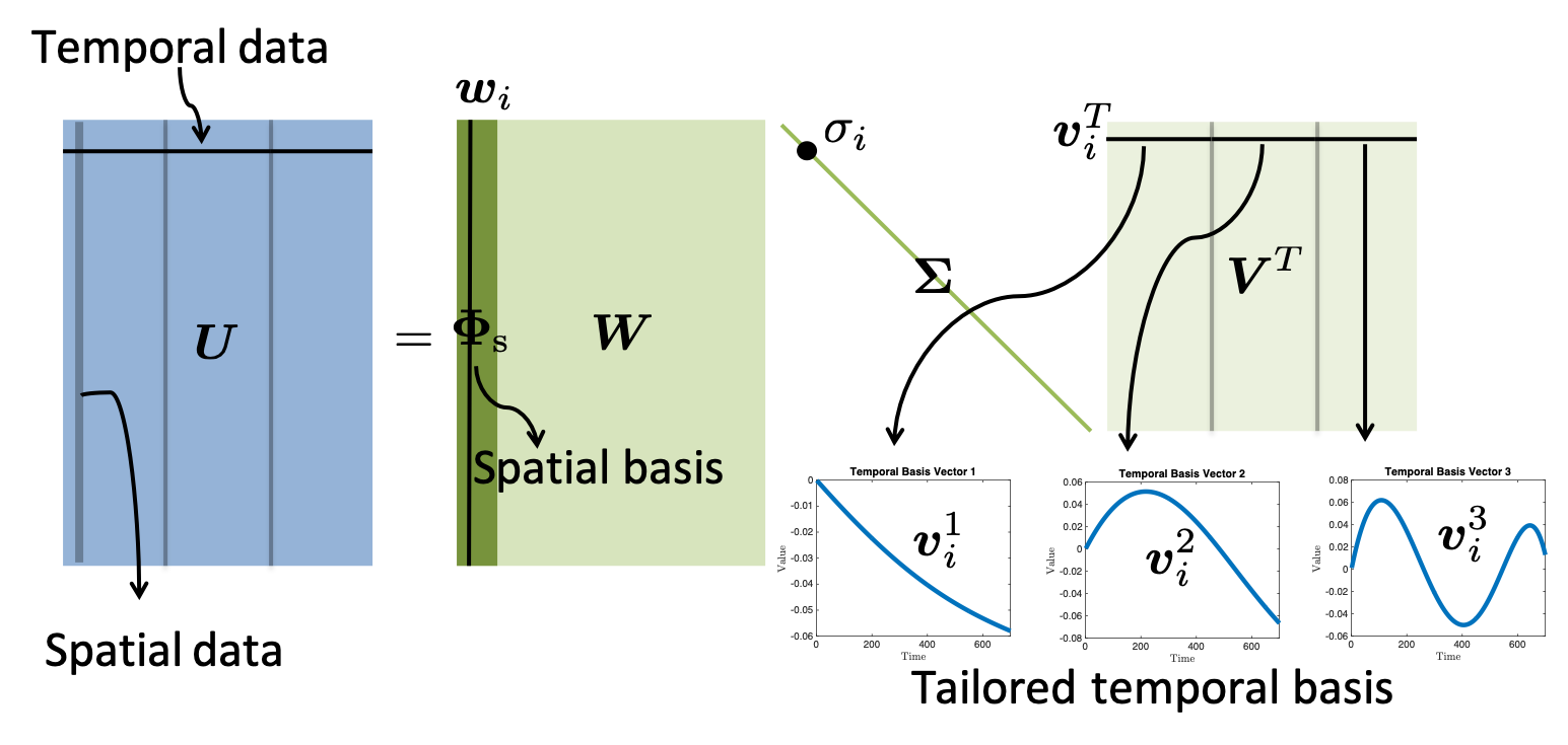
Figure 1: Illustration of spatial and temporal bases construction, using SVD with $n_{\mu}=3$. The right singular vector, $\boldsymbol{v}_{i}$, describes three different temporal behaviors of a left singular basis vector $\boldsymbol{w}_{i}$, i.e., three different temporal behaviors of a spatial mode. Each temporal behavior is denoted as $\boldsymbol{v}_{i}^{1}$, $\boldsymbol{v}_{i}^{2}$, and $\boldsymbol{v}_{i}^{3}$.

We follow the method of snapshots described by Sirovich [71]. First, let $\{\boldsymbol{\mu}_{1},\ldots,\boldsymbol{\mu}_{n_{\mu}}\}$ be a set of parameter samples, where we run full order model simulations. Let $\boldsymbol{U}_{p}\equiv\begin{bmatrix}\boldsymbol{u}^{(1)}(\boldsymbol{\mu}_{p})&\cdots&\boldsymbol{u}^{(N_{t})}(\boldsymbol{\mu}_{p})\end{bmatrix}\in\mathbb{R}^{N_{s}\times N_{t}}$, $p\in\mathbb{N}(n_{\mu})$, be a full order model solution matrix for a sample parameter, $\boldsymbol{\mu}_{p}\in\Omega_{\mu}$. Then concatenating all the solution matrix defines a snapshot matrix, $\boldsymbol{U}\in\mathbb{R}^{N_{s}\times n_{\mu}N_{t}}$, i.e.,

$$\boldsymbol{U}\equiv\begin{bmatrix}\boldsymbol{U}_{1}&\cdots&\boldsymbol{U}_{n_{\mu}}\end{bmatrix}.$$ (4.1)

We use Proper Orthogonal Decomposition (POD) to construct the spatial basis, $\boldsymbol{\Phi}_{\text{s}}$. POD [41] obtains $\boldsymbol{\Phi}_{\text{s}}$ by choosing the leading $n_{s}$ columns of the left singular matrix, $\boldsymbol{W}$, of the following Singular Value Decomposition (SVD) with $\ell\equiv\min(N_{s},n_{\mu}N_{t})$ and $n_{s}<n_{\mu}N_{t}$:

$$\boldsymbol{U} =\boldsymbol{W}\boldsymbol{\Sigma}\boldsymbol{V}^{T}$$ (4.2)

$$=\sum_{i=1}^{\ell}\sigma_{i}\boldsymbol{w}_{i}\boldsymbol{v}_{i}^{T},$$ (4.3)

where $\boldsymbol{W}\in\mathbb{R}^{N_{s}\times\ell}$ and $\boldsymbol{V}\in\mathbb{R}^{n_{\mu}N_{t}\times\ell}$ are orthogonal matrices and $\boldsymbol{\Sigma}\in\mathbb{R}^{\ell\times\ell}$ is a diagonal matrix with singular values on its diagonal. The spatial POD basis, $\boldsymbol{\Phi}_{\text{s}}$ minimizes

$$\left\|\boldsymbol{U}-\boldsymbol{\Phi}_{\text{s}}\boldsymbol{\Phi}_{\text{s}}^{T}{\boldsymbol{U}}\right\|_{F}^{2}$$ (4.4)

over all $\boldsymbol{\Phi}_{\text{s}}\in\mathbb{R}^{N_{s}\times n_{s}}$ with orthonormal columns, where $\|\cdot\|_{F}$ denotes the Frobenius norm. The POD procedure seeks the $n_{s}$-dimensional subspace that optimally represents the solution snapshot, $\boldsymbol{U}$. The equivalent summation form is written in (4.3), where $\sigma_{i}\in\mathbb{R}$ is $i$th singular value, $\boldsymbol{w}_{i}$ and $\boldsymbol{v}_{i}$ are $i$th left and right singular vectors, respectively. Note that $\boldsymbol{v}_{i}$ describes $n_{\mu}$ different temporal behavior of $\boldsymbol{w}_{i}$. For example, Figure 1 illustrates the case of $n_{\mu}=3$, where $\boldsymbol{v}_{i}^{1}$, $\boldsymbol{v}_{i}^{2}$, and $\boldsymbol{v}_{i}^{3}$ describe three different temporal behavior of a specific spatial basis vector, i.e., $\boldsymbol{w}_{i}$. For general $n_{\mu}$, we note that $\boldsymbol{v}_{i}$ describes $n_{\mu}$ different temporal behavior of $i$th spatial basis vector, i.e., $\boldsymbol{\phi}^{\text{s}}_{i}=\boldsymbol{w}_{i}$. We set $\boldsymbol{\Upsilon}_{i}=\begin{bmatrix}\boldsymbol{v}_{i}^{1}&\cdots&\boldsymbol{v}_{i}^{n_{\mu}}\end{bmatrix}$ to be $i$th temporal snapshot matrix, where $\boldsymbol{v}_{i}^{k}\equiv[\boldsymbol{v}_{i}(1+(k-1)N_{t}),\boldsymbol{v}_{i}(2+(k-1)N_{t}),\cdots,\boldsymbol{v}_{i}(kN_{t})]^{T}\in\mathbb{R}^{N_{t}}$ for $k\in\mathbb{N}(n_{\mu})$, where $\boldsymbol{v}_{i}(j),j\in\mathbb{N}(n_{\mu}N_{t})$ is the $j$th component of the vector. The SVD of $\boldsymbol{\Upsilon}_{i}$ is

$$\boldsymbol{\Upsilon}_{i}=\boldsymbol{\Lambda}_{i}\boldsymbol{\Sigma}_{i}\boldsymbol{\Psi}_{i}^{T}.$$ (4.5)

Then, choosing the leading $n_{t}$ vectors of $\boldsymbol{\Lambda}_{i}$ yields the temporal basis, $\boldsymbol{\Phi}_{\text{t}}^{i}$ for $i$th spatial basis vector. Finally, we can construct a space–time basis vector, $\boldsymbol{\phi}^{\text{st}}_{i+n_{s}(j-1)}\in\mathbb{R}^{N_{s}N_{t}}$, in Equation (3.2) as

$$\boldsymbol{\phi}^{\text{st}}_{i+n_{s}(j-1)}=\boldsymbol{\phi}^{\text{t}}_{ij}\otimes\boldsymbol{\phi}^{\text{s}}_{i},$$ (4.6)

where $\otimes$ denotes Kronecker product, $\boldsymbol{\phi}^{\text{s}}_{i}\in\mathbb{R}^{N_{s}}$ is $i$th vector of the spatial basis, $\boldsymbol{\Phi}_{\text{s}}$, and $\boldsymbol{\phi}^{\text{t}}_{ij}\in\mathbb{R}^{N_{t}}$ is $j$th vector of the temporal basis, $\boldsymbol{\Phi}_{\text{t}}^{i}$ that describes a temporal behavior of $\boldsymbol{\phi}^{\text{s}}_{i}$.

5 Space-time reduced order models in block structure

We avoid building the space–time basis vector defined in Equation (4.6) because it requires much memory for storage. Thus, we can exploit the block structure of the matrices to save computational cost and storage of the matrices in memory. Section 5.2 introduces such block structures for the space–time Galerkin projection, while Section 5.3 shows block structures for the space–time Petrov–Galerkin projection. First, we introduce common block structures that appear both the Galerkin and Petrov–Galerkin projections in Section 5.1.

5.1 Block structures of space–time basis

Following [1]’s notation, we define the block structure of the space–time basis to be:

$$\boldsymbol{\Phi}_{st}=\begin{pmatrix}\boldsymbol{\Phi}_{s}{\boldsymbol{D}}_{1}^{1}&\cdots&\cdots&\cdots&\boldsymbol{\Phi}_{s}{\boldsymbol{D}}_{1}^{n_{t}}\\ \vdots&\ddots&\vdots&\iddots&\vdots\\ \vdots&\cdots&\boldsymbol{\Phi}_{s}{\boldsymbol{D}}_{k}^{j}&\cdots&\vdots\\ \vdots&\iddots&\vdots&\ddots&\vdots\\ \boldsymbol{\Phi}_{s}{\boldsymbol{D}}_{N_{t}}^{1}&\cdots&\cdots&\cdots&\boldsymbol{\Phi}_{s}{\boldsymbol{D}}_{N_{t}}^{n_{t}}\end{pmatrix}\in\mathbb{R}^{N_{s}N_{t}\times n_{s}n_{t}}$$ (5.1)

where the $k$th time step of the temporal basis matrix is a diagonal matrix defined as

$${\boldsymbol{D}}_{k}^{j}=\begin{pmatrix}\phi_{1j,k}^{t}&0&\cdots&\cdots&0\\ 0&\ddots&0&\cdots&\vdots\\ \vdots&0&\phi_{ij,k}^{t}&\cdots&\vdots\\ \vdots&\vdots&\ddots&\ddots&0\\ 0&0&\cdots&0&\phi_{n_{s}j,k}^{t}\end{pmatrix}\in\mathbb{R}^{n_{s}\times n_{s}}$$ (5.2)

where $\phi_{ij,k}^{t}\in\mathbb{R}$ is the $k$th element of $\boldsymbol{\phi}_{ij}^{t}\in\mathbb{R}^{N_{t}}$.

5.2 Block structures of Galerkin projection

As shown in Table 1, the reduced space–time Galerkin system matrix, $\hat{{\boldsymbol{A}}}^{st,g}(\boldsymbol{\mu})$ is:

$$\hat{{\boldsymbol{A}}}^{st,g}(\boldsymbol{\mu})= \boldsymbol{\Phi}_{\text{st}}^{T}{\boldsymbol{A}}^{st}(\boldsymbol{\mu})\boldsymbol{\Phi}_{\text{st}}$$ (5.3)

Now, We define the block structure of this matrix as:

$$\hat{{\boldsymbol{A}}}^{st,g}(\boldsymbol{\mu})=\begin{pmatrix}\hat{{\boldsymbol{A}}}_{(1,1)}^{st,g}(\boldsymbol{\mu})&\cdots&\cdots&\cdots&\hat{{\boldsymbol{A}}}_{(1,n_{t})}^{st,g}(\boldsymbol{\mu})\\ \vdots&\ddots&\vdots&\iddots&\vdots\\ \vdots&\cdots&\hat{{\boldsymbol{A}}}^{st,pg}_{(j^{\prime},j)}(\boldsymbol{\mu})&\cdots&\vdots\\ \vdots&\iddots&\vdots&\ddots&\vdots\\ \hat{{\boldsymbol{A}}}_{(n_{t},1)}^{st,g}(\boldsymbol{\mu})&\cdots&\cdots&\cdots&\hat{{\boldsymbol{A}}}_{(n_{t},n_{t})}^{st,g}(\boldsymbol{\mu})\end{pmatrix}$$ (5.4)

so that we can exploit the block structure of these matrices such that we do not need to form the entire matrix. We derive that $\hat{{\boldsymbol{A}}}^{st,g}_{(j^{\prime},j)}(\boldsymbol{\mu})\in\mathbb{R}^{n_{s}\times n_{s}}$ where the $(j^{\prime},j)$th block matrix is:

$$\hat{{\boldsymbol{A}}}^{st,g}_{(j^{\prime},j)}(\boldsymbol{\mu})=\sum\limits_{k=1}^{N_{t}}\Big{(}{\boldsymbol{D}}_{k}^{j^{\prime}}{\boldsymbol{D}}_{k}^{j}-\Delta t^{(k)}{\boldsymbol{D}}_{k}^{j^{\prime}}\boldsymbol{\Phi}_{s}^{T}{\boldsymbol{A}}(\boldsymbol{\mu})\boldsymbol{\Phi}_{s}{\boldsymbol{D}}_{k}^{j}\Big{)}-\sum\limits_{k=1}^{N_{t}-1}{\boldsymbol{D}}_{k+1}^{j^{\prime}}{\boldsymbol{D}}_{k}^{j}$$ (5.5)

The reduced space–time Galerkin input vector $\hat{{\boldsymbol{f}}}^{st,g}(\boldsymbol{\mu})\in\mathbb{R}^{n_{s}n_{t}}$ is

$$\hat{{\boldsymbol{f}}}^{st,g}(\boldsymbol{\mu})=\boldsymbol{\Phi}_{\text{st}}^{T}\boldsymbol{f}^{\text{st}}(\boldsymbol{\mu}).$$ (5.6)

Again, utilizing the block structure of matrices, we compute $j$th block vector $\hat{{\boldsymbol{f}}}^{st,g}(\boldsymbol{\mu})_{(j)}\in\mathbb{R}^{n_{t}}$ to be:

$$\hat{{\boldsymbol{f}}}^{st,g}(\boldsymbol{\mu})_{(j)}=\sum\limits_{k=1}^{N_{t}}\Delta t^{(k)}{\boldsymbol{D}}_{k}^{j}\boldsymbol{\Phi}_{s}^{T}{\boldsymbol{B}}(\boldsymbol{\mu})\boldsymbol{f}^{(k)}(\boldsymbol{\mu}).$$ (5.7)

Finally, the space–time Galerkin initial vector, $\hat{{\boldsymbol{u}}_{0}}^{st,g}(\boldsymbol{\mu})\in\mathbb{R}^{n_{s}n_{t}}$, can be computed as:

$$\hat{{\boldsymbol{u}}_{0}}^{st,g}(\boldsymbol{\mu})=\boldsymbol{\Phi}_{\text{st}}^{T}\boldsymbol{u}_{0}^{\text{st}}(\boldsymbol{\mu})$$ (5.8)

where the $j$th block vector, $\hat{{\boldsymbol{u}}_{0}}^{st,g}(\boldsymbol{\mu})_{(j)}\in\mathbb{R}^{n_{s}}$, is:

$$\hat{{\boldsymbol{u}}_{0}}^{st,g}(\boldsymbol{\mu})_{(j)}={\boldsymbol{D}}_{1}^{j}\boldsymbol{\Phi}_{s}^{T}{\boldsymbol{u}}_{0}(\boldsymbol{\mu}).$$ (5.9)

5.3 Block structures of least-squares Petrov–Galerkin projection

As shown in Table 1, the reduced space–time Petrov–Galerkin system matrix, $\hat{{\boldsymbol{A}}}^{st,pg}(\boldsymbol{\mu})$ is:

$$\hat{{\boldsymbol{A}}}^{st,pg}(\boldsymbol{\mu})= \boldsymbol{\Phi}_{st}^{T}{\boldsymbol{A}}^{st}(\boldsymbol{\mu})^{T}{\boldsymbol{A}}^{st}(\boldsymbol{\mu})\boldsymbol{\Phi}_{st}$$ (5.10)

Now, We define the block structure of this matrix as:

$$\hat{{\boldsymbol{A}}}^{st,pg}(\boldsymbol{\mu})=\begin{pmatrix}\hat{{\boldsymbol{A}}}_{(1,1)}^{st,pg}(\boldsymbol{\mu})&\cdots&\cdots&\cdots&\hat{{\boldsymbol{A}}}_{(1,n_{t})}^{st,pg}(\boldsymbol{\mu})\\ \vdots&\ddots&\vdots&\iddots&\vdots\\ \vdots&\cdots&\hat{{\boldsymbol{A}}}^{st,pg}_{(j^{\prime},j)}(\boldsymbol{\mu})&\cdots&\vdots\\ \vdots&\iddots&\vdots&\ddots&\vdots\\ \hat{{\boldsymbol{A}}}_{(n_{t},1)}^{st,pg}(\boldsymbol{\mu})&\cdots&\cdots&\cdots&\hat{{\boldsymbol{A}}}_{(n_{t},n_{t})}^{st,pg}(\boldsymbol{\mu})\end{pmatrix}$$ (5.11)

so that we can exploit the block structure of these matrices such that we do not need to form the entire matrix. We derive that $\hat{{\boldsymbol{A}}}^{st,pg}_{(j^{\prime},j)}(\boldsymbol{\mu})\in\mathbb{R}^{n_{s}\times n_{s}}$ where the $(j^{\prime},j)$th block matrix is:

$$\hat{{\boldsymbol{A}}}^{st,pg}_{(j^{\prime},j)}(\boldsymbol{\mu})= \sum\limits_{k=1}^{N_{t}}\Big{[}{\boldsymbol{D}}_{k}^{j^{\prime}}\boldsymbol{\Phi}_{s}^{T}\Big{(}{\boldsymbol{I}}_{N_{s}}-\Delta t^{(k)}{\boldsymbol{A}}(\boldsymbol{\mu})^{T}\Big{)}\Big{(}{\boldsymbol{I}}_{N_{s}}-\Delta t^{(k)}{\boldsymbol{A}}(\boldsymbol{\mu})\Big{)}\boldsymbol{\Phi}_{s}{\boldsymbol{D}}_{k}^{j}\Big{]}$$ (5.12)

$$+\sum\limits_{k=1}^{N_{t}-1}\Big{[}{\boldsymbol{D}}_{k}^{j^{\prime}}{\boldsymbol{D}}_{k}^{j}-{\boldsymbol{D}}_{k}^{j^{\prime}}\boldsymbol{\Phi}_{s}^{T}\Big{(}{\boldsymbol{I}}_{N_{s}}-\Delta t^{(k+1)}{\boldsymbol{A}}(\boldsymbol{\mu})\Big{)}\boldsymbol{\Phi}_{s}{\boldsymbol{D}}_{k+1}^{j}$$

$$-{\boldsymbol{D}}_{k+1}^{j^{\prime}}\boldsymbol{\Phi}_{s}^{T}\Big{(}{\boldsymbol{I}}_{N_{s}}-\Delta t^{(k+1)}{\boldsymbol{A}}(\boldsymbol{\mu})^{T}\Big{)}\boldsymbol{\Phi}_{s}{\boldsymbol{D}}_{k}^{j}\Big{]}$$

The reduced space–time Petrov–Galerkin input vector $\hat{{\boldsymbol{f}}}^{st,pg}(\boldsymbol{\mu})\in\mathbb{R}^{n_{s}n_{t}}$ is

$$\hat{{\boldsymbol{f}}}^{st,pg}(\boldsymbol{\mu})=\boldsymbol{\Phi}_{st}^{T}{\boldsymbol{A}}^{st}(\boldsymbol{\mu})^{T}\boldsymbol{f}^{\text{st}}(\boldsymbol{\mu}).$$ (5.13)

Again, utilizing the block structure of matrices, we compute $j$th block vector $\hat{{\boldsymbol{f}}}^{st,pg}(\boldsymbol{\mu})_{(j)}\in\mathbb{R}^{n_{t}}$ to be:

$$\hat{{\boldsymbol{f}}}^{st,pg}(\boldsymbol{\mu})_{(j)}= \sum\limits_{k=1}^{N_{t}}\Big{[}{\boldsymbol{D}}_{k}^{j}\boldsymbol{\Phi}_{s}^{T}\Big{(}{\boldsymbol{I}}_{N_{s}}-\Delta t^{(k)}{\boldsymbol{A}}(\boldsymbol{\mu})^{T}\Big{)}\Delta t^{(k)}{\boldsymbol{B}}(\boldsymbol{\mu})\boldsymbol{f}^{(k)}(\boldsymbol{\mu})\Big{]}$$ (5.14)

$$-\sum\limits_{k=1}^{N_{t}-1}\Big{[}{\boldsymbol{D}}_{k}^{j}\boldsymbol{\Phi}_{s}^{T}\Delta t^{(k+1)}{\boldsymbol{B}}(\boldsymbol{\mu})\boldsymbol{f}^{(k+1)}(\boldsymbol{\mu})\Big{]}.$$

Finally, the space–time Petrov–Galerkin initial vector, $\hat{{\boldsymbol{u}}_{0}}^{st,pg}(\boldsymbol{\mu})\in\mathbb{R}^{n_{s}n_{t}}$, can be computed as:

$$\hat{{\boldsymbol{u}}_{0}}^{st,pg}(\boldsymbol{\mu})=\boldsymbol{\Phi}_{st}^{T}{\boldsymbol{A}}^{st}(\boldsymbol{\mu})^{T}\boldsymbol{u}_{0}^{\text{st}}(\boldsymbol{\mu})$$ (5.15)

where the $j$th block vector, $\hat{{\boldsymbol{u}}_{0}}^{st,pg}(\boldsymbol{\mu})_{(j)}\in\mathbb{R}^{n_{s}}$, is:

$$\hat{{\boldsymbol{u}}_{0}}^{st,pg}(\boldsymbol{\mu})_{(j)}={\boldsymbol{D}}_{1}^{j}\boldsymbol{\Phi}_{s}^{T}\Big{(}{\boldsymbol{I}}_{N_{s}}-\Delta t^{(1)}{\boldsymbol{A}}(\boldsymbol{\mu})^{T}\Big{)}{\boldsymbol{u}}_{0}(\boldsymbol{\mu}).$$ (5.16)

5.4 Comparison of Galerkin and Petrov–Galerkin block structures

The block structures of space–time reduced order model operators are summarized in Table 2.

Table 2: Comparison of Galerkin and Petrov–Galerkin block structures

Galerkin	Petrov–Galerkin
$\hat{{\boldsymbol{A}}}^{st,g}(\boldsymbol{\mu})_{(j^{\prime},j)}=$	$\hat{{\boldsymbol{A}}}^{st,pg}(\boldsymbol{\mu})_{(j^{\prime},j)}=$
$\sum\limits_{k=1}^{N_{t}}\Big{(}{\boldsymbol{D}}_{k}^{j^{\prime}}{\boldsymbol{D}}_{k}^{j}-\Delta t^{(k)}{\boldsymbol{D}}_{k}^{j^{\prime}}\boldsymbol{\Phi}_{s}^{T}{\boldsymbol{A}}(\boldsymbol{\mu})\boldsymbol{\Phi}_{s}{\boldsymbol{D}}_{k}^{j}\Big{)}$	$\sum\limits_{k=1}^{N_{t}}\Big{[}{\boldsymbol{D}}_{k}^{j^{\prime}}\boldsymbol{\Phi}_{s}^{T}\Big{(}{\boldsymbol{I}}_{N_{s}}-\Delta t^{(k)}{\boldsymbol{A}}(\boldsymbol{\mu})^{T}\Big{)}\Big{(}{\boldsymbol{I}}_{N_{s}}-\Delta t^{(k)}{\boldsymbol{A}}(\boldsymbol{\mu})\Big{)}\boldsymbol{\Phi}_{s}{\boldsymbol{D}}_{k}^{j}\Big{]}$
$-\sum\limits_{k=1}^{N_{t}-1}{\boldsymbol{D}}_{k+1}^{j^{\prime}}{\boldsymbol{D}}_{k}^{j}$	$+\sum\limits_{k=1}^{N_{t}-1}\Big{[}{\boldsymbol{D}}_{k}^{j^{\prime}}{\boldsymbol{D}}_{k}^{j}-{\boldsymbol{D}}_{k}^{j^{\prime}}\boldsymbol{\Phi}_{s}^{T}\Big{(}{\boldsymbol{I}}_{N_{s}}-\Delta t^{(k+1)}{\boldsymbol{A}}(\boldsymbol{\mu})\Big{)}\boldsymbol{\Phi}_{s}{\boldsymbol{D}}_{k+1}^{j}$
	$-{\boldsymbol{D}}_{k+1}^{j^{\prime}}\boldsymbol{\Phi}_{s}^{T}\Big{(}{\boldsymbol{I}}_{N_{s}}-\Delta t^{(k+1)}{\boldsymbol{A}}(\boldsymbol{\mu})^{T}\Big{)}\boldsymbol{\Phi}_{s}{\boldsymbol{D}}_{k}^{j}\Big{]}$
$\hat{{\boldsymbol{f}}}^{st,g}(\boldsymbol{\mu})_{(j)}=$	$\hat{{\boldsymbol{f}}}^{st,pg}(\boldsymbol{\mu})_{(j)}=\sum\limits_{k=1}^{N_{t}}\Big{[}{\boldsymbol{D}}_{k}^{j}\boldsymbol{\Phi}_{s}^{T}\Big{(}{\boldsymbol{I}}_{N_{s}}-\Delta t^{(k)}{\boldsymbol{A}}(\boldsymbol{\mu})^{T}\Big{)}\Delta t^{(k)}{\boldsymbol{B}}(\boldsymbol{\mu})\boldsymbol{f}^{(k)}(\boldsymbol{\mu})\Big{]}$
$\sum\limits_{k=1}^{N_{t}}{\boldsymbol{D}}_{k}^{j}\Delta t^{(k)}\boldsymbol{\Phi}_{s}^{T}{\boldsymbol{B}}(\boldsymbol{\mu})\boldsymbol{f}^{(k)}(\boldsymbol{\mu})$	$-\sum\limits_{k=1}^{N_{t}-1}\Big{[}{\boldsymbol{D}}_{k}^{j}\boldsymbol{\Phi}_{s}^{T}\Delta t^{(k+1)}{\boldsymbol{B}}(\boldsymbol{\mu})\boldsymbol{f}^{(k+1)}(\boldsymbol{\mu})\Big{]}$
$\hat{{\boldsymbol{u}}_{0}}^{st,g}(\boldsymbol{\mu})_{(j)}={\boldsymbol{D}}_{1}^{j}\boldsymbol{\Phi}_{s}^{T}{\boldsymbol{u}}_{0}(\boldsymbol{\mu})$	$\hat{{\boldsymbol{u}}_{0}}^{st,pg}(\boldsymbol{\mu})_{(j)}={\boldsymbol{D}}_{1}^{j}\boldsymbol{\Phi}_{s}^{T}\Big{(}{\boldsymbol{I}}_{N_{s}}-\Delta t^{(1)}{\boldsymbol{A}}(\boldsymbol{\mu})^{T}\Big{)}{\boldsymbol{u}}_{0}(\boldsymbol{\mu})$

5.5 Computational complexity of forming space–time ROM operators

To compute computational complexity of forming the reduced space–time system matrices, input vectors, and initial state vectors for Galerkin and Petrov–Galerkin projections, we assume that ${\boldsymbol{A}}(\boldsymbol{\mu})\in\mathbb{R}^{N_{s}\times N_{s}}$ is a band matrix with the bandwidth, $b$ and ${\boldsymbol{B}}(\boldsymbol{\mu})$ is a identity matrix, ${\boldsymbol{I}}_{N_{s}}$. The band structure of ${\boldsymbol{A}}(\boldsymbol{\mu})$ is often seen in mathematical models because of local approximations to derivative terms. Then, the bandwidth of ${\boldsymbol{A}}^{st}(\boldsymbol{\mu})\in\mathbb{R}^{N_{s}N_{t}\times N_{s}N_{t}}$ formed with backward Euler scheme is $N_{s}$. We also assume that the spatial basis vectors $\boldsymbol{\phi}^{\text{s}}_{i}\in\mathbb{R}^{N_{s}},i\in\mathbb{N}(n_{s})$ and temporal basis vectors $\boldsymbol{\phi}^{\text{t}}_{ij}\in\mathbb{R}^{N_{t}},i\in\mathbb{N}(n_{s})\text{ and }j\in\mathbb{N}(n_{t})$ are given.

Let us start to compute the computational cost without use of block structures. Constructing space–time basis costs $\mathcal{O}(N_{s}N_{t}n_{s}n_{t})$. For Galerkin projections, computing the reduced space–time system matrix, input vectors, and initial state vector costs $\mathcal{O}(2N_{s}^{2}N_{t}n_{s}n_{t})+\mathcal{O}(N_{s}N_{t}(n_{s}n_{t})^{2})$, $\mathcal{O}(N_{s}N_{t}n_{s}n_{t})$, and $\mathcal{O}(N_{s}n_{s}n_{t})$, respectively. Thus, keeping the dominant terms and taking off coefficient $2$ lead to $\mathcal{O}(N_{s}^{2}N_{t}n_{s}n_{t})+\mathcal{O}(N_{s}N_{t}(n_{s}n_{t})^{2})$. With the assumption of $n_{s}n_{t}\ll N_{s}$, we have $\mathcal{O}(N_{s}^{2}N_{t}n_{s}n_{t})$. For Petrov–Galerkin projections, we first compute $\boldsymbol{\Phi}_{\text{st}}^{T}{\boldsymbol{A}}^{st}(\boldsymbol{\mu})$, resulting in $\mathcal{O}(2N_{s}^{2}N_{t}n_{s}n_{t})$. Then, computing the reduced space–time system matrix, input vectors, and initial state vector costs $\mathcal{O}(N_{s}N_{t}(n_{s}n_{t})^{2})$, $\mathcal{O}(N_{s}N_{t}n_{s}n_{t})$, and $\mathcal{O}(N_{s}n_{s}n_{t})$, respectively. Thus, keeping the dominant terms and taking off coefficient $2$ lead to $\mathcal{O}(N_{s}^{2}N_{t}n_{s}n_{t})+\mathcal{O}(N_{s}N_{t}(n_{s}n_{t})^{2})$. With the assumption of $n_{s}n_{t}\ll N_{s}$, we have $\mathcal{O}(N_{s}^{2}N_{t}n_{s}n_{t})$.

Now, let us compute the computational complexity with use of block structures. For Galerkin projection, we first compute $\boldsymbol{\Phi}_{s}^{T}{\boldsymbol{A}}(\boldsymbol{\mu})\boldsymbol{\Phi}_{s}$ which will be reused, resulting in $\mathcal{O}(2bN_{s}n_{s})+\mathcal{O}(N_{s}n_{s}^{2})$. Then, we compute $n_{t}^{2}$ blocks for the reduced space–time system matrix. It takes $\mathcal{O}(N_{t}(2n_{s}^{2}+2n_{s}))$ to compute each block. Thus, it costs $\mathcal{O}(N_{t}n_{t}^{2}(2n_{s}^{2}+2n_{s}))$ to compute the reduced space–time system matrix. For the reduced space–time input vector, $n_{t}$ blocks are needed and each block costs $\mathcal{O}(N_{t}(N_{s}n_{s}+n_{s}))$, resulting in $\mathcal{O}(N_{t}n_{t}(N_{s}n_{s}+n_{s}))$. The computing the reduced space–time initial vector costs $\mathcal{O}(N_{s}n_{s}+n_{s})$. Thus, keeping the dominant terms and taking off coefficient $2$ lead to $\mathcal{O}(bN_{s}n_{s})+\mathcal{O}(N_{s}n_{s}^{2})+\mathcal{O}(N_{t}(n_{s}n_{t})^{2})+\mathcal{O}(N_{s}N_{t}n_{s}n_{t})$. With the assumptions of $b\ll N_{t}n_{t}$, $n_{s}\ll N_{t}n_{t}$, and $n_{s}n_{t}\ll N_{s}$, we have $\mathcal{O}(N_{s}N_{t}n_{s}n_{t})$. For Petrov–Galerkin projection, we compute $({\boldsymbol{I}}_{N_{s}}-\Delta t{\boldsymbol{A}}(\boldsymbol{\mu}))\boldsymbol{\Phi}_{s}$, resulting in $\mathcal{O}(2bN_{s}n_{s})$. Then, we compute $\boldsymbol{\Phi}_{s}^{T}({\boldsymbol{I}}_{N_{s}}-\Delta t{\boldsymbol{A}}(\boldsymbol{\mu})^{T})({\boldsymbol{I}}_{N_{s}}-\Delta t{\boldsymbol{A}}(\boldsymbol{\mu}))\boldsymbol{\Phi}_{s}$ and $\boldsymbol{\Phi}_{s}^{T}({\boldsymbol{I}}_{N_{s}}-\Delta t{\boldsymbol{A}}(\boldsymbol{\mu}))\boldsymbol{\Phi}_{s}$ for re-use. Each of them costs $\mathcal{O}(N_{s}n_{s}^{2})$. Now, we compute $n_{t}^{2}$ blocks for the reduced space–time system matrix. It takes $\mathcal{O}(N_{t}(6n_{s}^{2}+n_{s}))$ to compute each block. Thus, it costs $\mathcal{O}(N_{t}n_{t}^{2}(6n_{s}^{2}+n_{s}))$ to compute the reduced space–time system matrix. For the reduced space–time input vector, $n_{t}$ blocks are needed and each block costs $\mathcal{O}(N_{t}(N_{s}n_{s}+n_{s}))$, resulting in $\mathcal{O}(N_{t}n_{t}(N_{s}n_{s}+n_{s}))$. The computing the reduced space–time initial vector costs $\mathcal{O}(N_{s}n_{s}+n_{s})$. Thus, keeping the dominant terms and taking off coefficients $2$ and $6$ lead to $\mathcal{O}(bN_{s}n_{s})+\mathcal{O}(N_{s}n_{s}^{2})+\mathcal{O}(N_{t}(n_{s}n_{t})^{2})+\mathcal{O}(N_{s}N_{t}n_{s}n_{t})$. With the assumptions of $b\ll N_{t}n_{t}$, $n_{s}\ll N_{t}n_{t}$, and $n_{s}n_{t}\ll N_{s}$, we have $\mathcal{O}(N_{s}N_{t}n_{s}n_{t})$.

In summary, the computational complexities of forming space–time ROM operators in training phase for Galerkin and Petrov–Galerkin projections are presented in Table 3. We observe that a lot of computational costs are reduced by making use of block structures for forming space–time reduced order models.

Table 3: Comparison of Galerkin and Petrov–Galerkin computational complexities

	Galerkin	Petrov–Galerkin
Not using block structures	$\mathcal{O}(N_{s}^{2}N_{t}n_{s}n_{t})$	$\mathcal{O}(N_{s}^{2}N_{t}n_{s}n_{t})$
Using block structures	$\mathcal{O}(N_{s}N_{t}n_{s}n_{t})$	$\mathcal{O}(N_{s}N_{t}n_{s}n_{t})$

6 Error analysis

We present error analysis of the space–time ROM method. The error analysis is based on [1]. A posteriori error bound is derived in this section. Here, we drop the parameter dependence for notational simplicity.

Theorem 6.1.

We define the error at $k$th time step as $\boldsymbol{e}^{(k)}\equiv\boldsymbol{u}^{(k)}-\tilde{\boldsymbol{u}}^{(k)}\in\mathbb{R}^{N_{s}}$ where $\boldsymbol{u}^{(k)}\in\mathbb{R}^{N_{s}}$ denotes FOM solution, $\tilde{\boldsymbol{u}}^{(k)}\in\mathbb{R}^{N_{s}}$ denotes approximate solution, and $k\in\mathbb{N}(N_{t})$. Let $\boldsymbol{A}^{\text{st}}\in\mathbb{R}^{N_{s}N_{t}\times N_{s}N_{t}}$ be the space–time system matrix, $\boldsymbol{r}^{(k)}\in\mathbb{R}^{N_{s}}$ be the residual computed using FOM solution at $k$th time step, and $\tilde{\boldsymbol{r}}^{(k)}\in\mathbb{R}^{N_{s}}$ be the residual computed using approximate solution at $k$th time step. For example, $\boldsymbol{r}^{(k)}$ and $\tilde{\boldsymbol{r}}^{(k)}$ after applying the backward Euler scheme with the uniform time step become

$$\boldsymbol{r}^{(k)}(\boldsymbol{u}^{(k)},\boldsymbol{u}^{(k-1)}) =\Delta t\boldsymbol{f}^{(k)}+\boldsymbol{u}^{(k-1)}-(\boldsymbol{I}-\Delta t\boldsymbol{A})\boldsymbol{u}^{(k)}=\boldsymbol{0}$$ (6.1)

$$\tilde{\boldsymbol{r}}^{(k)}(\tilde{\boldsymbol{u}}^{(k)},\tilde{\boldsymbol{u}}^{(k-1)}) =\Delta t\boldsymbol{f}^{(k)}+\tilde{\boldsymbol{u}}^{(k-1)}-(\boldsymbol{I}-\Delta t\boldsymbol{A})\tilde{\boldsymbol{u}}^{(k)}$$ (6.2)

with $\tilde{\boldsymbol{u}}^{(0)}=\boldsymbol{u}^{0}$. Then, the error bound is given by

$$\max_{k\in\mathbb{N}(N_{t})}\|\boldsymbol{e}^{(k)}\|_{2}\leq\eta\max_{k\in\mathbb{N}(N_{t})}\|\tilde{\boldsymbol{r}}^{(k)}\|_{2}$$ (6.3)

where $\eta\equiv\sqrt{N_{t}}\|(\boldsymbol{A}^{\text{st}})^{-1}\|_{2}$ denotes the stability constant.

Proof.

Let us define the space–time residual as

$$\boldsymbol{r}^{\text{st}}:\boldsymbol{v}\mapsto\boldsymbol{f}^{\text{st}}+\boldsymbol{u}_{0}^{\text{st}}-\boldsymbol{A}^{\text{st}}\boldsymbol{v}$$ (6.4)

with $\boldsymbol{r}^{\text{st}}:\mathbb{R}^{N_{s}N_{t}}\rightarrow\mathbb{R}^{N_{s}N_{t}}$. Then, we have

$$\boldsymbol{r}^{\text{st}}(\boldsymbol{u}^{\text{st}}) =\boldsymbol{f}^{\text{st}}+\boldsymbol{u}_{0}^{\text{st}}-\boldsymbol{A}^{\text{st}}\boldsymbol{u}^{\text{st}}=\boldsymbol{0}$$ (6.5)

$$\boldsymbol{r}^{\text{st}}(\tilde{\boldsymbol{u}}^{\text{st}}) =\boldsymbol{f}^{\text{st}}+\boldsymbol{u}_{0}^{\text{st}}-\boldsymbol{A}^{\text{st}}\tilde{\boldsymbol{u}}^{\text{st}}$$ (6.6)

where $\boldsymbol{u}^{\text{st}}\in\mathbb{R}^{N_{s}N_{t}}$ is the space–time FOM solution and $\tilde{\boldsymbol{u}}^{\text{st}}\in\mathbb{R}^{N_{s}N_{t}}$ is the approximate space–time solution. Subtracting Equation (6.6) from Equation (6.5) gives

$$\boldsymbol{r}^{\text{st}}(\tilde{\boldsymbol{u}}^{\text{st}})=\boldsymbol{A}^{\text{st}}\boldsymbol{e}^{st}$$ (6.7)

where $\boldsymbol{e}^{st}\equiv\boldsymbol{u}^{\text{st}}-\tilde{\boldsymbol{u}}^{\text{st}}\in\mathbb{R}^{N_{s}N_{t}}$. Inverting $\boldsymbol{A}^{\text{st}}$ yields

$$\boldsymbol{e}^{st}=(\boldsymbol{A}^{\text{st}})^{-1}\boldsymbol{r}^{\text{st}}(\tilde{\boldsymbol{u}}^{\text{st}}).$$ (6.8)

Taking $\ell_{2}$ norm and Hölders’ inequality gives

$$\|\boldsymbol{e}^{st}\|_{2}\leq\|(\boldsymbol{A}^{\text{st}})^{-1}\|_{2}\|\boldsymbol{r}^{\text{st}}(\tilde{\boldsymbol{u}}^{\text{st}})\|_{2}.$$ (6.9)

We can re-write this in the following form

$$\sqrt{\sum_{k=1}^{N_{t}}\|\boldsymbol{e}^{(k)}\|_{2}^{2}}\leq\|(\boldsymbol{A}^{\text{st}})^{-1}\|_{2}\sqrt{\sum_{k=1}^{N_{t}}\|\tilde{\boldsymbol{r}}^{(k)}\|_{2}^{2}}.$$ (6.10)

Using the relations

$$\max_{k\in\mathbb{N}(N_{t})}\|\boldsymbol{e}^{(k)}\|_{2}^{2}\leq\sum_{k=1}^{N_{t}}\|\boldsymbol{e}^{(k)}\|_{2}^{2}$$ (6.11)

and

$$\sum_{k=1}^{N_{t}}\|\tilde{\boldsymbol{r}}^{(k)}\|_{2}^{2}\leq N_{t}\max_{k\in\mathbb{N}(N_{t})}\|\tilde{\boldsymbol{r}}^{(k)}\|_{2}^{2},$$ (6.12)

we have

$$\max_{k\in\mathbb{N}(N_{t})}\|\boldsymbol{e}^{(k)}\|_{2}\leq\sqrt{N_{t}}\|(\boldsymbol{A}^{\text{st}})^{-1}\|_{2}\max_{k\in\mathbb{N}(N_{t})}\|\tilde{\boldsymbol{r}}^{(k)}\|_{2},$$ (6.13)

which is equivalent to the error bound in (6.3). ∎

A numerical demonstration with space–time system matrices, $\boldsymbol{A}^{\text{st}}$ that have the same structure as the ones used in Section 7.1 and Section 7.2.1 shows the magnitude of $\|(\boldsymbol{A}^{\text{st}})^{-1}\|_{2}$ increases linearly for small $N_{t}$, while it becomes eventually flattened for large $N_{t}$ as shown in Fig. 2(a) for the backward Euler time integrator with uniform time step size. Combined with $\sqrt{N_{t}}$, the stability constant $\eta$ growth rate is shown in Fig. 2(b). These error bound shows much improvement against the ones for the spatial Galerkin and Petrov–Galerkin ROMs, which grows exponentially in time [1].

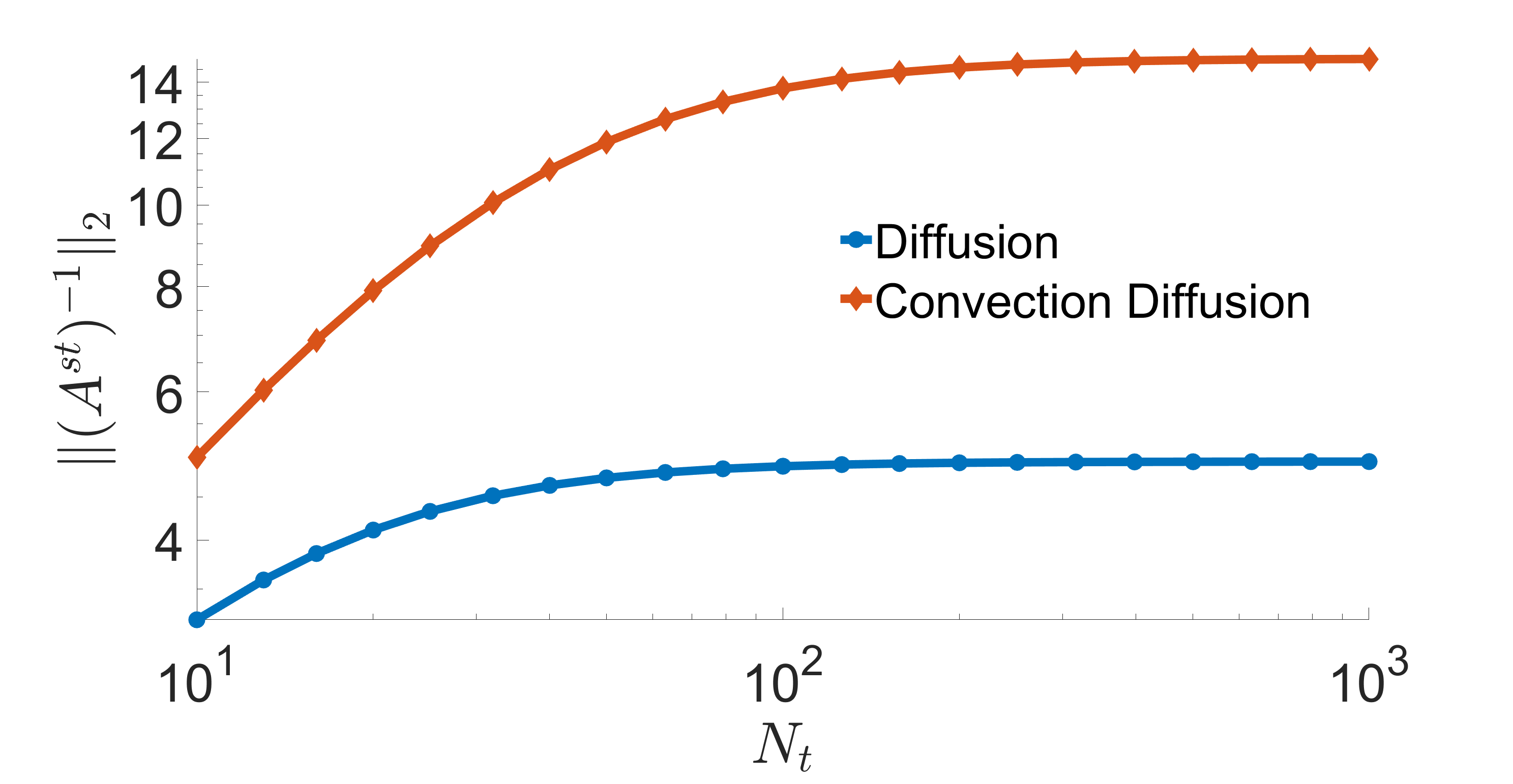
(a) $\|(\boldsymbol{A}^{\text{st}})^{-1}\|_{2}$ in inequality (6.3)

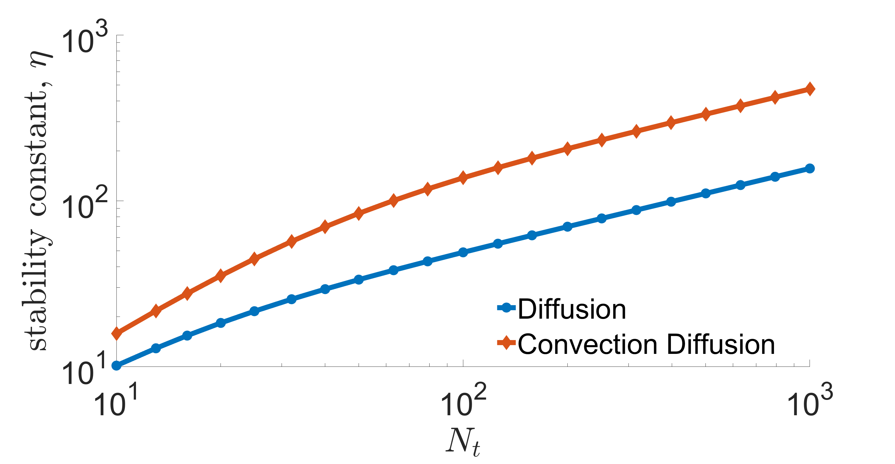
(b) Stability constant, $\eta$ in inequality (6.3)

Figure 2: Growth rate of stability constant in Theorem 6.1. Backward Euler time stepping scheme with uniform time step size, $\Delta t=10^{-2}$ is used.

7 Numerical results

In this section, we apply both the space–time Galerkin and Petrov–Galerkin ROMs to two model problems: (i) a 2D linear diffusion equation in Section 7.1 and (ii) a 2D linear convection-diffusion equation in Section 7.2. We demonstrate their accuracy and speed-up. The space–time ROMs are trained with solution snapshots associated with parameters in a chosen domain and used to predict the solution of a parameter that is not included in the trained parameter domain. We refer to this as the predictive case. The accuracy of space–time ROM solution $\tilde{\boldsymbol{u}}^{\text{st}}(\boldsymbol{\mu})$ is assessed from its relative error by:

$$\text{relative error}=\frac{\left\|\tilde{\boldsymbol{u}}^{\text{st}}(\boldsymbol{\mu})-\boldsymbol{u}^{\text{st}}(\boldsymbol{\mu})\right\|_{2}}{\left\|\boldsymbol{u}^{\text{st}}(\boldsymbol{\mu})\right\|_{2}}$$ (7.1)

and the $\ell_{2}$ norm of space–time residual:

$$\left\|\boldsymbol{r}^{\text{st}}(\tilde{\boldsymbol{u}}^{\text{st}}(\boldsymbol{\mu}))\right\|_{2}.$$ (7.2)

The computational cost is measured in terms of CPU wall-clock time. The online speed-up is evaluated by dividing the wall-clock time of the FOM by the online phase of the ROM. For the multi-query problems, total speed-up is evaluated by dividing the time of all FOMs by the time of all ROMs including training time. All calculations are performed on an Intel(R) Core(TM) i9-10900T CPU @ 1.90GHz and DDR4 Memory @ 2933MHz.

7.1 2D linear diffusion equation

We consider a parameterized 2D linear diffusion equation with a source term

$$\begin{split}\frac{\partial u}{\partial t}=\left[\frac{\partial^{2}u}{\partial x^{2}}+\frac{\partial^{2}u}{\partial y^{2}}\right]&-\left[\frac{1}{\sqrt{(x-\mu_{1})^{2}+(y-\mu_{2})^{2}}}\right]u\\ &+\frac{\sin{2\pi t}}{\sqrt{(x-\mu_{1})^{2}+(y-\mu_{2})^{2}}}\end{split}$$ (7.3)

where $(x,y)\in[0,1]\times[0,1]$, $t\in[0,2]$ and $(\mu_{1},\mu_{2})\in[-1.7,-0.2]\times[-1.7,-0.2]$. The boundary condition is

$$u(x=0,y,t) =0$$ (7.4)

$$u(x=1,y,t) =0$$

$$u(x,y=0,t) =0$$

$$u(x,y=1,t) =0$$

and the initial condition is

$$u(x,y,t=0)=0.$$ (7.5)

The backward Euler with uniform time step size $\frac{2}{N_{t}}$ is employed, where we set $N_{t}=50$. For spatial differentiation, the second order central difference scheme is implemented for the diffusion terms. Discretizing the space domain into $N_{x}=70$ and $N_{y}=70$ uniform meshes in $x$ and $y$ directions, respectively, gives $N_{s}=(N_{x}-1)\times(N_{y}-1)=4,761$ grid points, excluding boundary grid points. As a result, there are $238,050$ free degrees of freedom in space–time.

For training phase, we collect solution snapshots associated with the following parameters:

$$(\mu_{1},\mu_{2})\in\{(-0.9,-0.9),(-0.9,-0.5),(-0.5,-0.9),(-0.5,-0.5)\}$$

at which the FOM is solved.

The Galerkin and Petrov–Galerkin space–time ROMs solve the Equation (7.3) with the target parameter $(\mu_{1},\mu_{2})=(-0.7,-0.7))$. Fig. 3,  4, and 5 show the relative errors, the space–time residuals, and the online speed-ups as a function of the reduced dimension $n_{s}$ and $n_{t}$. We observe that both Galerkin and Petrov–Galerkin ROMs with $n_{s}=5$ and $n_{t}=3$ achieve a good accuracy (i.e., relative errors of 0.012% and 0.026%, respectively) and speed-up (i.e., 350.31 and 376.04, respectively). We also observe that the relative errors of Galerkin projection is smaller but the space–time residual is larger than Petrov–Galerkin projection. This is because Petrov–Galerkin space–time ROM solution minimizes the space–time residual.

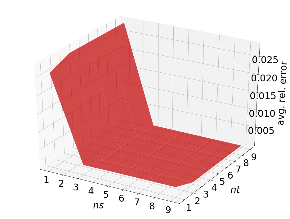
(a) Relative errors vs reduced dimensions for Galerkin projection

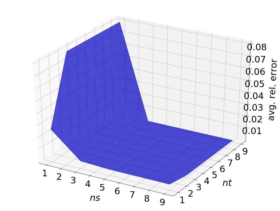
(b) Relative errors vs reduced dimensions for Petrov–Galerkin projection

Figure 3: 2D linear diffusion equation. Relative errors vs reduced dimensions.

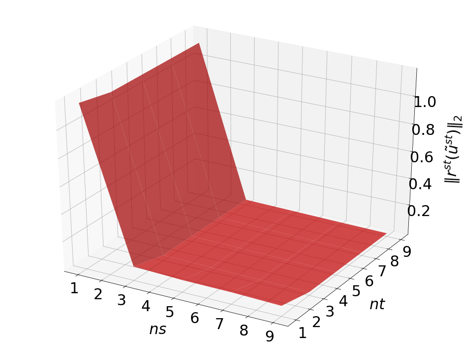
(a) Space-time residuals vs reduced dimensions for Galerkin projection

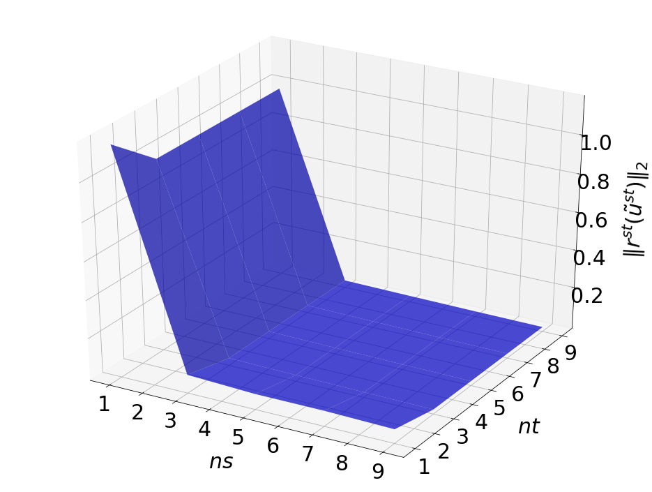
(b) Space-time residuals vs reduced dimensions for Petrov–Galerkin projection

Figure 4: 2D linear diffusion equation. Space-time residuals vs reduced dimensions.

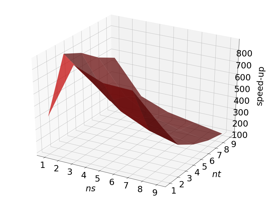
(a) Speedups vs reduced dimensions for Galerkin projection

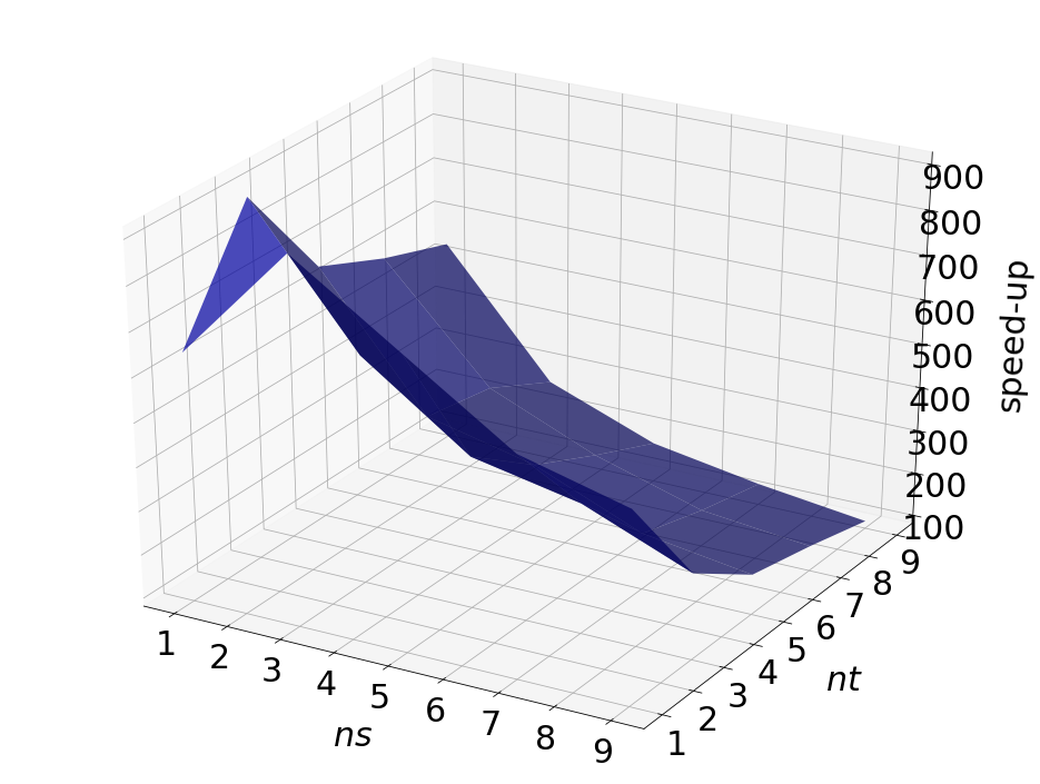
(b) Speedups vs reduced dimensions for Petrov–Galerkin projection

Figure 5: 2D linear diffusion equation. Speedups vs reduced dimensions.

The final time snapshots of FOM, Galerkin space–time ROM, and Petrov–Galerkin space–time ROM are seen in Fig. 6. Both ROMs have a basis size of $n_{s}=5$ and $n_{t}=3$, resulting in a reduction factor of $(N_{s}N_{t})\small/(n_{s}n_{t})=15,870$. For the Galerkin method, the FOM and space–time ROM simulation with $n_{s}=5$ and $n_{t}=3$ takes an average time of $6.1816\times 10^{-1}$ and $1.7646\times 10^{-3}$ seconds, respectively, resulting in speed-up of $350.31$. For the Petrov–Galerkin method, the FOM and space–time ROM simulation with $n_{s}=5$ and $n_{t}=3$ takes an average time of $6.0809\times 10^{-1}$ and $1.6171\times 10^{-3}$ seconds, respectively, resulting in speed-up of $376.04$. For accuracy, the Galerkin method results in $1.210\times 10^{-2}$ % relative error and $1.249\times 10^{-2}$ space–time residual norm while the Petrov–Galerkin results in $2.626\times 10^{-2}$ % relative error and $1.029\times 10^{-2}$ space–time residual norm.

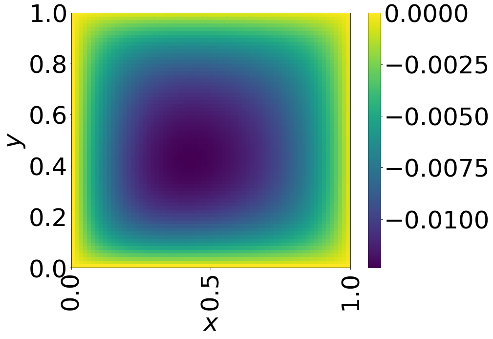
(a) FOM

(b) Galerkin ROM

(c) Petrov–Galerkin ROM

Figure 6: Solution snapshots of FOM, Galerkin ROM, and Petrov–Galerkin ROM at $t=2$.

We investigate the numerical tests to see the generalization capability of both Galerkin and Petrov–Galerkin ROMs. The train parameter set, $(\mu_{1},\mu_{2})\in\{(-0.9,-0.9),(-0.9,-0.5),(-0.5,-0.9),(-0.5,-0.5)\}$ is used to train a space–time ROMs with a basis of $n_{s}=5$ and $n_{t}=3$. Then trained ROMs solve predictive cases with the test parameter set, $(\mu_{1},\mu_{2})\in\{\mu_{1}|\mu_{1}=-1.7+1.5\small/14i,i=0,1,\cdots,14\}\times\{\mu_{2}|\mu_{2}=-1.7+1.5\small/14j,j=0,1,\cdots,14\}$. Fig. 7 shows the relative errors over the test parameter set. The Galerkin and Petrov–Galerkin ROMs are the most accurate within the range of the train parameter points, i.e., $[-0.9,-0.5]\times[-0.9,-0.5]$. As the parameter points go beyond the train parameter domain, the accuracy of the Galerkin and Petrov–Galerkin ROMs start to deteriorate gradually. This implies that the Galerkin and Petrov–Galerkin ROMs have a trust region. Its trust region should be determined by the application space. For Galerkin ROM, online speed-up is about $389$ in average and total time for ROM and FOM are $107.14$ and $132.66$ seconds, respectively, resulting in total speed-up of $1.24$. For Petrov–Galerkin ROM, online speed-up is about $386$ in average and total time for ROM and FOM are $117.96$ and $132.42$ seconds, respectively, resulting in total speed-up of $1.12$. Since the training time doesn’t depend on the number of test cases, we expect more speed-up for a larger number of test cases.

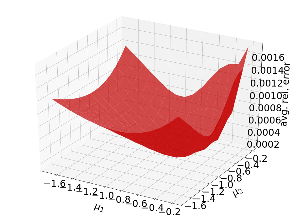
(a) Glaerkin

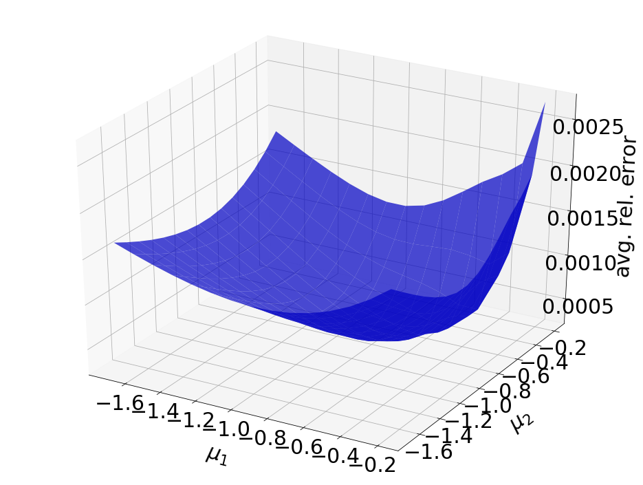
(b) Petrov–Galerkin

Figure 7: The comparison of the Galerkin and Petrov–Galerkin ROMs for predictive cases

7.2 2D linear convection diffusion equation

7.2.1 Without source term

We consider a parameterized 2D linear convection diffusion equation

$$\frac{\partial u}{\partial t}=-\mu_{1}\left[\frac{\partial u}{\partial x}+\frac{\partial u}{\partial y}\right]+\mu_{2}\left[\frac{\partial^{2}u}{\partial x^{2}}+\frac{\partial^{2}u}{\partial y^{2}}\right]$$ (7.6)

where $(x,y)\in[0,1]\times[0,1]$, $t\in[0,1]$ and $(\mu_{1},\mu_{2})\in[0.01,0.07]\times[0.31,0.37]$. The boundary condition is given by

$$u(x=0,y,t) =0$$ (7.7)

$$u(x=1,y,t) =0$$

$$u(x,y=0,t) =0$$

$$u(x,y=1,t) =0.$$

The initial condition is given by

$$u(x,y,t=0)=\left\{\begin{array}[]{ll}100\sin{(2\pi x)}^{3}\cdot\sin{(2\pi y)}^{3}&\text{if }(x,y)\in[0,0.5]\times[0,0.5]\\ 0&\text{otherwise}\end{array}\right.$$ (7.10)

and shown in Fig. 8.

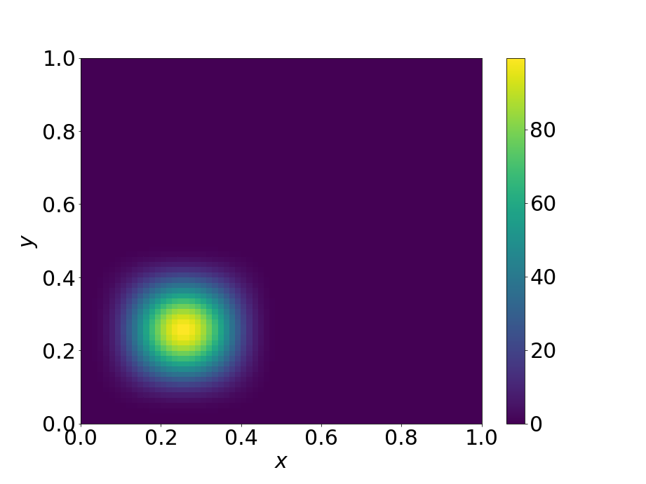
Figure 8: Plot of Equation (7.10)

The backward Euler with uniform time step size $\frac{1}{N_{t}}$ is employed where we set $N_{t}=50$. For spatial differentiation, a second order central difference scheme for the diffusion terms and a first order backward difference scheme for the convection terms are implemented. Discretizing the space domain into $N_{x}=70$ and $N_{y}=70$ uniform meshes in $x$ and $y$ directions, respectively, gives $N_{s}=(N_{x}-1)\times(N_{y}-1)=4,761$ grid points, excluding boundary grid points. As a result, there are $238,050$ free degrees of freedom in space–time.

For training phase, we collect solution snapshots associated with the following parameters:

$$(\mu_{1},\mu_{2})\in\{(0.03,0.33),(0.03,0.35),(0.05,0.33),(0.05,0.35)\},$$

at which the FOM is solved.

The Galerkin and Petrov–Galerkin space–time ROMs solve the Equation (7.6) with the target parameter $(\mu_{1},\mu_{2})=(0.04,0.34)$. Fig. 9,  10, and 11 show the relative errors, the space–time residuals, and the online speed-ups as a function of the reduced dimension $n_{s}$ and $n_{t}$. We observe that both Galerkin and Petrov–Galerkin ROMs with $n_{s}=5$ and $n_{t}=3$ achieve a good accuracy (i.e., relative errors of 0.049% and 0.059%, respectively) and speed-up (i.e., 451.17 and 370.74, respectively). We also observe that the relative errors of Galerkin projection is smaller but the space–time residual is larger than Petrov–Galerkin projection. This is because Petrov–Galerkin space–time ROM solution minimizes the space–time residual.

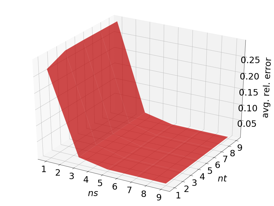
(a) Relative errors vs reduced dimensions for Galerkin projection

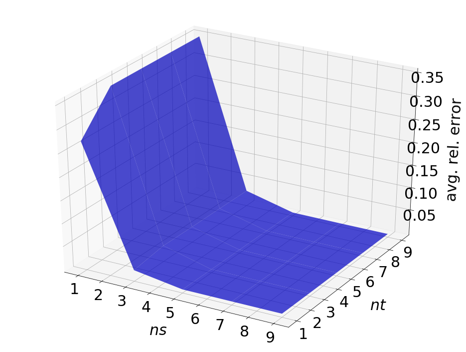
(b) Relative errors vs reduced dimensions for Petrov–Galerkin projection

Figure 9: 2D linear convection diffusion equation. Relative errors vs reduced dimensions.

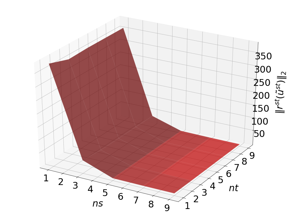
(a) Space-time residuals vs reduced dimensions for Galerkin projection

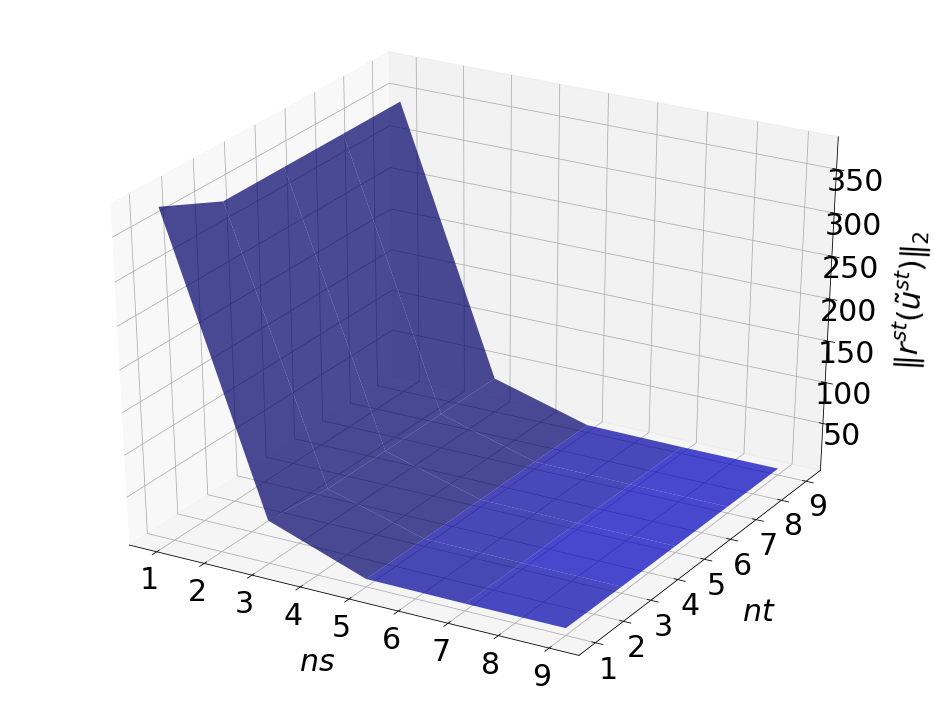
(b) Space-time residuals vs reduced dimensions for Petrov–Galerkin projection

Figure 10: 2D linear convection diffusion equation. Space-time residuals vs reduced dimensions.

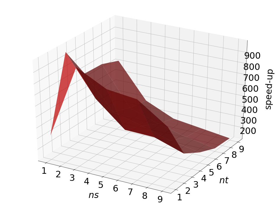
(a) Speedups vs reduced dimensions for Galerkin projection

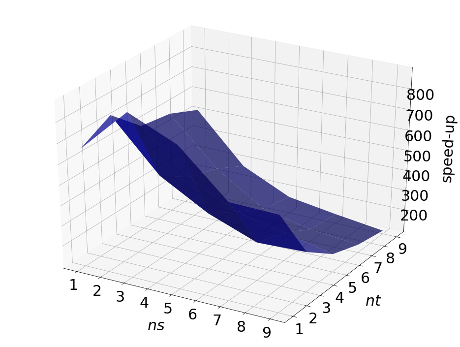
(b) Speedups vs reduced dimensions for Petrov–Galerkin projection

Figure 11: 2D linear convection diffusion equation. Speedups vs reduced dimensions.

The final time snapshots of FOM, Galerkin space–time ROM, and Petrov–Galerkin space–time ROM are seen in Fig. 12. Both ROMs have a basis size of $n_{s}=5$ and $n_{t}=3$, resulting in a reduction factor of $(N_{s}N_{t})\small/(n_{s}n_{t})=15,870$. For the Galerkin method, the FOM and space–time ROM simulation with $n_{s}=5$ and $n_{t}=3$ takes an average time of $6.1562\times 10^{-1}$ and $1.3645\times 10^{-3}$ seconds, respectively, resulting in speed-up of $451.17$. For the Petrov–Galerkin method, the FOM and space–time ROM simulation with $n_{s}=5$ and $n_{t}=3$ takes an average time of $5.7617\times 10^{-1}$ and $1.5541\times 10^{-3}$ seconds, respectively, resulting in speed-up of $370.74$. For accuracy, the Galerkin method results in $4.898\times 10^{-2}$ % relative error and $1.503$ space–time residual norm while the Petrov–Galerkin results in $5.878\times 10^{-2}$ % relative error and $1.459$ space–time residual norm.

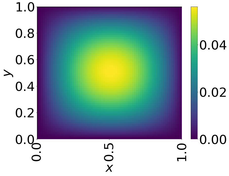
(a) FOM

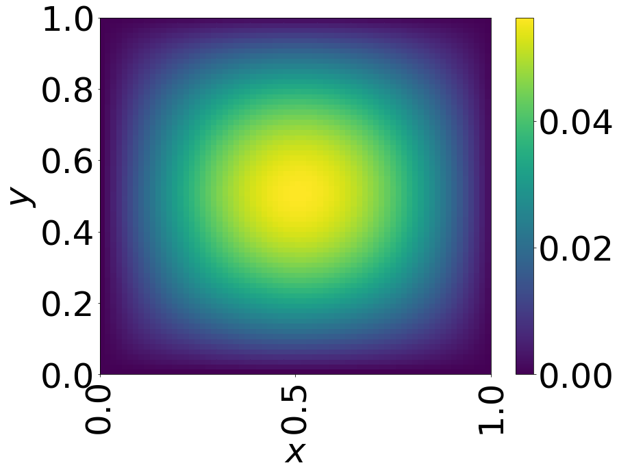
(b) Galerkin ROM

(c) Petrov–Galerkin ROM

Figure 12: Solution snapshots of FOM, Galerkin ROM, and Petrov–Galerkin ROM at $t=1$.

We investigate the numerical tests to see the generalization capability of both Galerkin and Petrov–Galerkin ROMs. The train parameter set, $(\mu_{1},\mu_{2})\in\{(0.03,0.33),(0.03,0.35),(0.05,0.33),(0.05,0.35)\}$ is used to train a space–time ROMs with a basis of $n_{s}=5$ and $n_{t}=3$. Then trained ROMs solve predictive cases with the test parameter set, $(\mu_{1},\mu_{2})\in\{\mu_{1}|\mu_{1}=0.01+0.06\small/11i,i=0,1,\cdots,11\}\times\{\mu_{2}|\mu_{2}=0.31+0.06\small/11j,j=0,1,\cdots,11\}$. Fig. 13 shows the relative errors over the test parameter set. The Galerkin and Petrov–Galerkin ROMs are the most accurate within the range of the train parameter points, i.e., $[0.03,0.33]\times[0.05,0.35]$. As the parameter points go beyond the train parameter domain, the accuracy of the Galerkin and Petrov–Galerkin ROMs start to deteriorate gradually. This implies that the Galerkin and Petrov–Galerkin ROMs have a trust region. Its trust region should be determined by an application. For Galerkin ROM, online speed-up is about $387$ in average and total time for ROM and FOM are $65.03$ and $83.89$ seconds, respectively, resulting in total speed-up of $1.29$. For Petrov–Galerkin ROM, online speed-up is about $385$ in average and total time for ROM and FOM are $70.55$ and $83.34$ seconds, respectively, resulting in total speed-up of $1.18$. Since the training time doesn’t depend on the number of test cases, we expect more speed-up for the larger number of test cases.

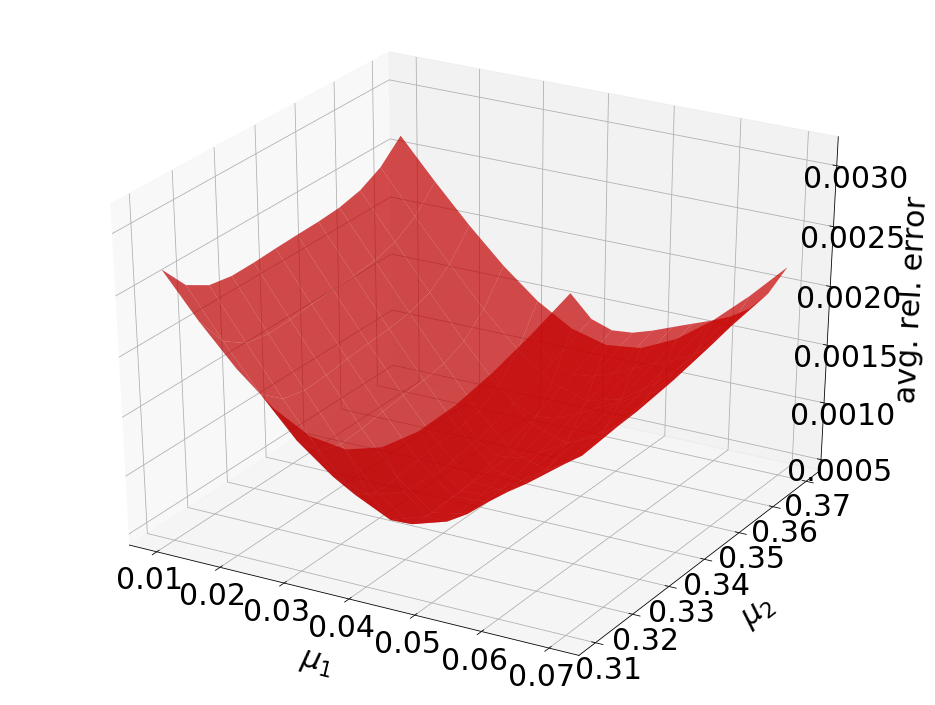
(a) Glaerkin

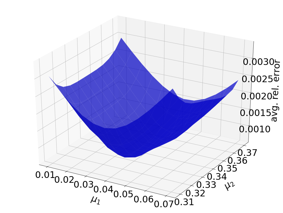
(b) Petrov–Galerkin

Figure 13: The comparison of the Galerkin and Petrov–Galerkin ROMs for predictive cases

7.2.2 With source term

We consider a parameterized 2D linear convection diffusion equation

$$\frac{\partial u}{\partial t}=-\mu_{1}\left[0.1\frac{\partial u}{\partial x}+\frac{\partial u}{\partial y}\right]+\mu_{2}\left[\frac{\partial^{2}u}{\partial x^{2}}+\frac{\partial^{2}u}{\partial y^{2}}\right]+f(x,y,t)$$ (7.11)

with the source term $f(x,y,t)$ which is given by

$$f(x,y,t)=10^{5}\exp(-((\frac{x-0.5+0.2\sin{(2\pi t})}{0.1})^{2}+(\frac{y}{0.05})^{2}))$$ (7.12)

where $(x,y)\in[0,1]\times[0,1]$, $t\in[0,2]$ and $(\mu_{1},\mu_{2})\in[0.195,0.205]\times[0.018,0.022]$. The boundary condition is given by

$$u(x=0,y,t) =0$$ (7.13)

$$u(x=1,y,t) =0$$

$$u(x,y=0,t) =0$$

$$u(x,y=1,t) =0$$

and the initial condition is given by

$$u(x,y,t=0)=0.$$ (7.14)

The backward Euler with uniform time step size $\frac{2}{N_{t}}$ is employed where we set $N_{t}=50$. For spatial differentiation, a second order central difference scheme for the diffusion terms and a first order backward difference scheme for the convection terms are implemented. Discretizing the space domain into $N_{x}=70$ and $N_{y}=70$ uniform meshes in $x$ and $y$ directions, respectively, gives $N_{s}=(N_{x}-1)\times(N_{y}-1)=4,761$ grid points, excluding boundary grid points. As a result, there are $238,050$ free degrees of freedom in space–time.

For training phase, we collect solution snapshots associated with the following parameters:

$$(\mu_{1},\mu_{2})\in\{(0.195,0.018),(0.195,0.022),(0.205,0.018),(0.205,0.022)\},$$

at which the FOM is solved.

The Galerkin and Petrov–Galerkin space–time ROMs solve the Equation (7.11) with the target parameter $(\mu_{1},\mu_{2})=(0.2,0.02))$. Fig. 14,  15, and 16 show the relative errors, the space–time residuals, and the online speed-ups as a function of the reduced dimension $n_{s}$ and $n_{t}$. We observe that both Galerkin and Petrov–Galerkin ROMs with $n_{s}=19$ and $n_{t}=3$ achieve a good accuracy (i.e., relative errors of 0.217% and 0.265%, respectively) and speed-up (i.e., 153.87 and 139.88, respectively). We also observe that the relative errors of Galerkin projection is smaller but the space–time residual is larger than Petrov–Galerkin projection. This is because Petrov–Galerkin space–time ROM solution minimizes the space–time residual.

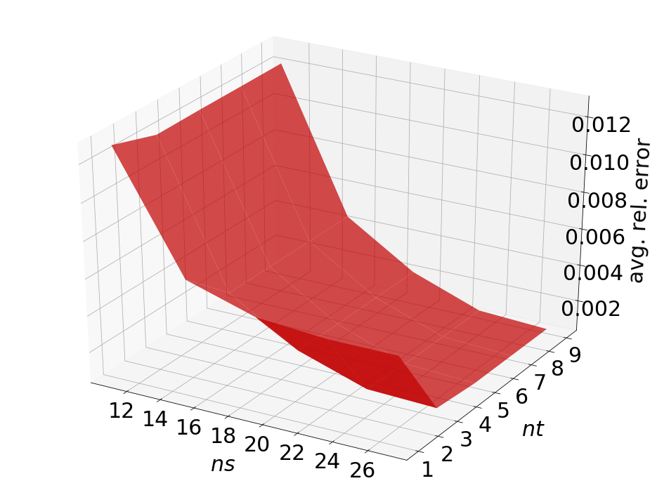
(a) Relative errors vs reduced dimensions for Galerkin projection

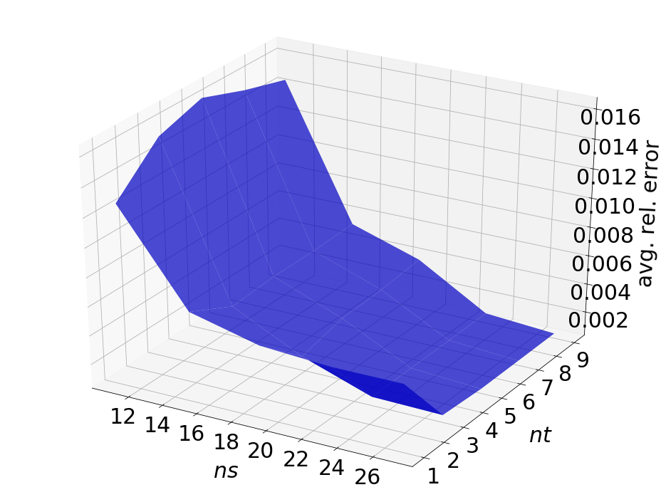
(b) Relative errors vs reduced dimensions for Petrov–Galerkin projection

Figure 14: 2D linear convection diffusion equation with source term. Relative errors vs reduced dimensions.

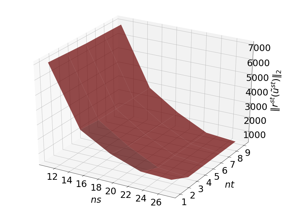
(a) Space-time residuals vs reduced dimensions for Galerkin projection

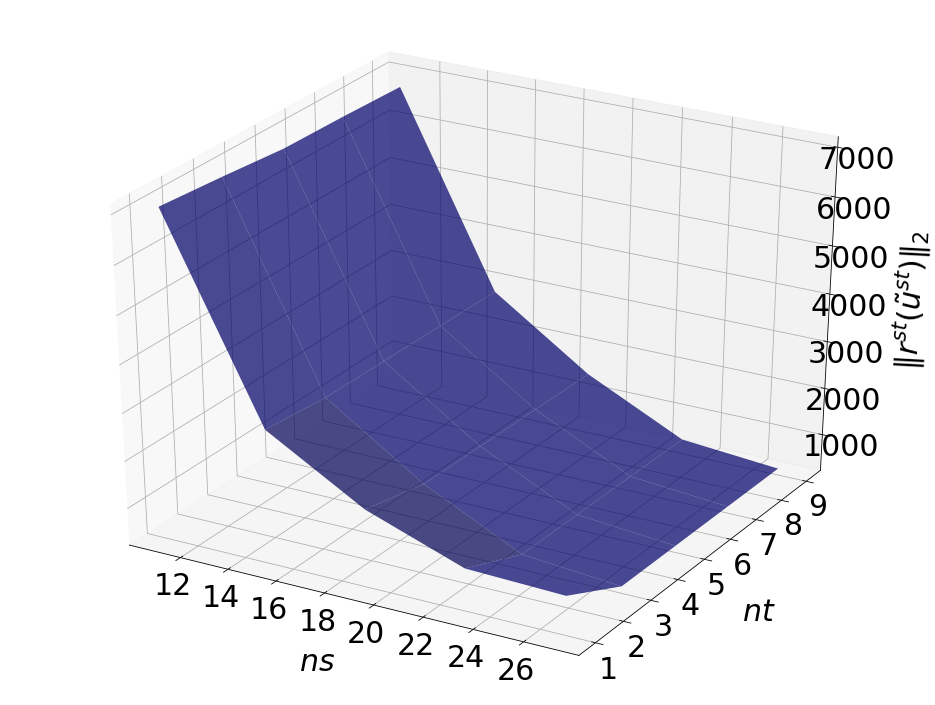
(b) Space-time residuals vs reduced dimensions for Petrov–Galerkin projection

Figure 15: 2D linear convection diffusion equation with source term. Space-time residuals vs reduced dimensions.

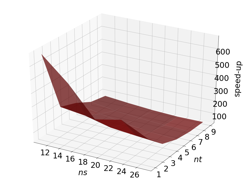
(a) Speedups vs reduced dimensions for Galerkin projection

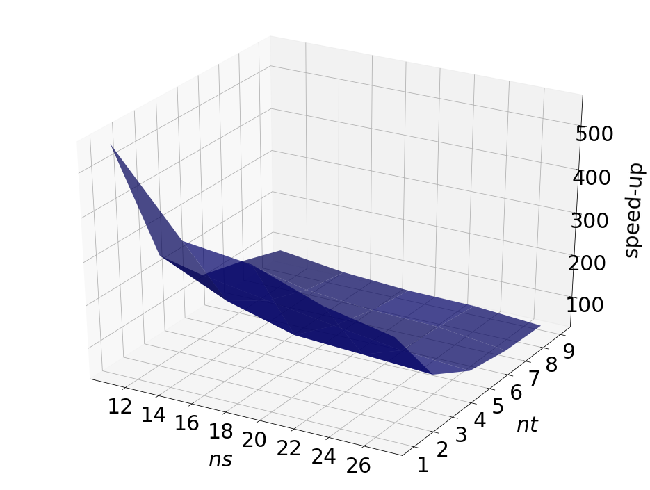
(b) Speedups vs reduced dimensions for Petrov–Galerkin projection

Figure 16: 2D linear convection diffusion equation with source term. Speedups vs reduced dimensions.

The final time snapshots of FOM, Galerkin space–time ROM, and Petrov–Galerkin space–time ROM are seen in Fig. 17. Both ROMs have a basis size of $n_{s}=19$ and $n_{t}=3$, resulting in a reduction factor of $(N_{s}N_{t})\small/(n_{s}n_{t})=4,176$. For the Galerkin method, the FOM and space–time ROM simulation with $n_{s}=19$ and $n_{t}=3$ takes an average time of $6.1209\times 10^{-1}$ and $3.9780\times 10^{-3}$ seconds, respectively, resulting in speed-up of $153.87$. For the Petrov–Galerkin method, the FOM and space–time ROM simulation with $n_{s}=19$ and $n_{t}=3$ takes an average time of $5.8780\times 10^{-1}$ and $4.2020\times 10^{-3}$ seconds, respectively, resulting in speed-up of $139.89$. For accuracy, the Galerkin method results in $2.174\times 10^{-1}$ % relative error and $1.564\times 10^{3}$ space–time residual norm while the Petrov–Galerkin results in $2.652\times 10^{-1}$ % relative error and $1.550\times 10^{3}$ space–time residual norm.

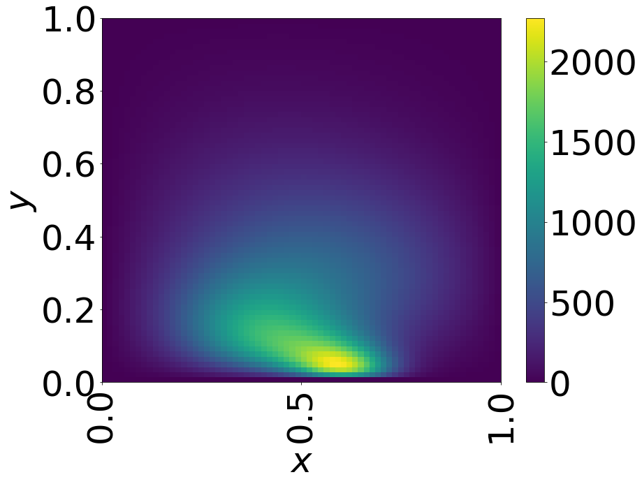
(a) FOM

(b) Galerkin ROM

(c) Petrov–Galerkin ROM

Figure 17: Solution snapshots of FOM, Galerkin ROM, and Petrov–Galerkin ROM at $t=2$.

We investigate the numerical tests to see the generalization capability of both Galerkin and Petrov–Galerkin ROMs. The train parameter set, $(\mu_{1},\mu_{2})\in\{(0.195,0.018),(0.195,0.022),(0.205,0.018),(0.205,0.022)\}$ is used to train a space–time ROMs with a basis of $n_{s}=19$ and $n_{t}=3$. Then trained ROMs solve predictive cases with the test parameter set, $(\mu_{1},\mu_{2})\in\{\mu_{1}|\mu_{1}=0.160+0.08\small/11i,i=0,1,\cdots,11\}\times\{\mu_{2}|\mu_{2}=0.016+0.008\small/11j,j=0,1,\cdots,11\}$. Fig. 18 shows the relative errors over the test parameter set. The Galerkin and Petrov–Galerkin ROMs are the most accurate within the range of the train parameter points, i.e., $[0.195,0.205]\times[0.018,0.022]$. As the parameter points go beyond the train parameter domain, the accuracy of the Galerkin and Petrov–Galerkin ROMs start to deteriorate gradually. This implies that the Galerkin and Petrov–Galerkin ROMs have a trust region. Its trust region should be determined by an application. For Galerkin ROM, online speed-up is about $133$ in average and total time for ROM and FOM are $68.49$ and $82.35$ seconds, respectively, resulting in total speed-up of $1.20$. For Petrov–Galerkin ROM, online speed-up is about $138$ in average and total time for ROM and FOM are $75.75$ and $86.04$ seconds, respectively, resulting in total speed-up of $1.14$. Since the training time doesn’t depend on the number of test cases, we expect more speed-up for the larger number of test cases.

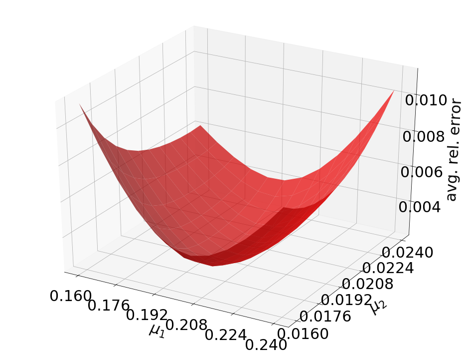
(a) Glaerkin

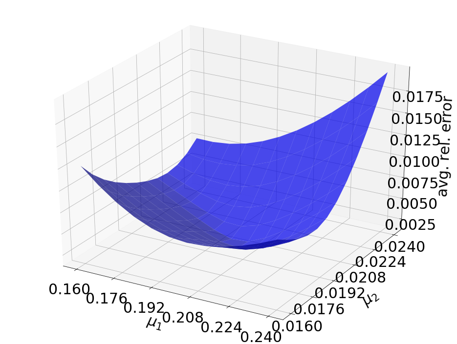
(b) Petrov–Galerkin

Figure 18: The comparison of the Galerkin and Petrov–Galerkin ROMs for predictive cases

8 Conclusion

In this work, we have formulated Galerkin and Petrov–Galerkin space–time ROMs using block structures which enable us to implement the space–time ROM operators efficiently. We also presented an a posteriori error bound for both Galerkin and Petrov–Galerkin space–time ROMs. We demonstrated that both Galerkin and Petrov–Galerkin space–time ROMs solves 2D linear diffusion problems and 2D linear convection diffusion problems accurately and efficiently. Both space–time reduced order models were able to achieve $\mathcal{O}(10^{-3})$ to $\mathcal{O}(10^{-4})$ relative errors with $\mathcal{O}(10^{2})$ speed-ups. We also presented our Python codes used for the numerical examples in Appendix A so that readers can easily reproduce our numerical results. Furthermore, each Python code is less than 120 lines, demonstrating the ease of implementing our space–time ROMs.

We used a linear subspace based ROM which is suitable for accelerating physical simulations whose solution space has a small Kolmogorov $n$-width. However, the linear subspace based ROM is not able to represent advection-dominated or sharp gradient solutions with a small number of bases. To address this challenge, a nonlinear manifold based ROM can be used, and recently, a nonlinear manifold based ROM has been developed for spatial ROMs [72, 73]. In future work, we aim to develop a nonlinear manifold based space–time ROM.

Appendix A Python codes in less than 120 lines of code for all numerical models described in Section 7

The Python code used for the numerical examples described in this paper are included in the following pages of the appendix are listed below. The total number of lines in each of the files are denoted in the parentheses. Note that we removed print statements of the results.

1. All input code for the Galerkin Reduced Order Model for 2D Implicit Linear Diffusion Equation with Source Term (111 lines)

2. All input code for the Petrov–Galerkin Reduced Order Model for 2D Implicit Linear Diffusion Equation with Source Term (117 lines)

3. All input code for the Galerkin Reduced Order Model for 2D Implicit Linear Convection Diffusion Equation (114 lines)

4. All input code for the Petrov–Galerkin Reduced Order Model for 2D Implicit Linear Convection Diffusion Equation (116 lines)

5. All input code for the Galerkin Reduced Order Model for 2D Implicit Linear Convection Diffusion Equation with Source Term (115 lines)

6. All input code for the Petrov–Galerkin Reduced Order Model for 2D Implicit Linear Convection Diffusion Equation with Source Term (119 lines)

A.1 Galerkin Reduced Order Model for 2D Implicit Linear Diffusion Equation with Source Term

    

1 import numpy as np; import scipy as sp 

2 from scipy.sparse.linalg import spsolve 

3  

4 # train parameter space 

5 mu1,mu2=np.meshgrid(np.linspace(-0.9,-0.5,2),np.linspace(-0.9,-0.5,2),indexing=’ij’) 

6 mu1=mu1.flatten(); mu2=mu2.flatten(); no_para=np.size(mu1,axis=0) 

7  

8 # space and time domain 

9 N=70; Ns=(N-1)**2; Nt=50; h=1/N; k=2/Nt 

10 x1,x2=np.meshgrid(np.linspace(0,1,N+1)[1:-1],np.linspace(0,1,N+1)[1:-1],indexing=’ij’) 

11 x1=x1.flatten(); x2=x2.flatten(); t=np.linspace(0,2,Nt+1) 

12  

13 # basic operators 

14 e=np.ones(N-1); I=sp.sparse.eye(Ns,format=’csc’) 

15 A1D=1/h**2*sp.sparse.spdiags(np.vstack((e,-2*e,e)),[-1,0,1],N-1,N-1,format=’csc’) 

16 A2D=sp.sparse.kron(A1D,sp.sparse.eye(N-1,format=’csc’),format=’csc’)\ 

17     +sp.sparse.kron(sp.sparse.eye(N-1,format=’csc’),A1D,format=’csc’) 

18  

19 # snapshot, free DoFs, No IC included 

20 U=np.zeros((Ns,no_para*Nt)) 

21 for p in range(no_para): 

22     A=A2D-sp.sparse.diags(1/np.sqrt((x1-mu1[p])**2+(x2-mu2[p])**2),format=’csc’) 

23     f=(1/np.sqrt((x1-mu1[p])**2+(x2-mu2[p])**2).reshape(-1,1))@(np.sin(2*np.pi*t).reshape(1,-1)) 

24     u=np.zeros((Ns,Nt+1)) # IC is zero 

25     for n in range(Nt): 

26         u[:,n+1]=spsolve(I-k*A,u[:,n]+k*f[:,n+1]) 

27     U[:,np.arange(p*Nt,(p+1)*Nt)]=u[:,1:] 

28  

29 W,S,VT=np.linalg.svd(U) # POD of solution snapshot 

30  

31 # test parameter space 

32 nparam1=15; nparam2=15; ParamD1,ParamD2=np.meshgrid(np.linspace(-1.7,-0.2,nparam1),np.linspace(-1.7,-0.2,nparam2)) 

33 ParamD1=ParamD1.flatten(); ParamD2=ParamD2.flatten(); num_test=np.prod(ParamD1.shape) 

34  

35 # variables to store (also store ParamD1 and ParamD2) 

36 UROM_g2=np.zeros((num_test,Nt+1,N+1,N+1)); UFOM_2=np.zeros((num_test,Nt+1,N+1,N+1)) 

37 AvgRelErr_g2=np.zeros((num_test)); STResROM_g2=np.zeros((num_test)) 

38  

39 # Construct Phi_s 

40 ns=5; PHIs=W[:,:ns]; PHIsT=PHIs.T 

41  

42 # construct Djk 

43 nt=3; D=np.zeros((ns,nt*Nt)) 

44 for i in range(ns): 

45     Ri=VT[i,:]; Ri=Ri.reshape(-1,no_para,order=’F’) 

46     Wi,Si,ViT=np.linalg.svd(Ri); PHIti=Wi[:,:nt] 

47     for j in range(nt): 

48         D[i,Nt*j:Nt*(j+1)]=PHIti[:,j] 

49  

50 # construct PHIst for post processing, i.e., reconstruction 

51 PHIst=np.zeros((Ns*Nt,ns*nt)) 

52 for i in range(Nt): 

53     for j in range(nt): 

54         PHIstij=np.zeros((Ns,ns)) 

55         Dij=sp.sparse.diags(D[:,j*Nt+i],format=’csc’) 

56         PHIst[Ns*i:Ns*(i+1),ns*j:ns*(j+1)]=PHIs@Dij 

57 PHIstT=PHIst.T 

58  

59 for test_count in range(num_test): # predictive cases 

60     param1,param2=ParamD1[test_count],ParamD2[test_count] # set parameter 

61  

62     # set model 

63     A=A2D-sp.sparse.diags(1/np.sqrt((x1-param1)**2+(x2-param2)**2),format=’csc’) 

64     f=(1/np.sqrt((x1-param1)**2+(x2-param2)**2).reshape(-1,1))@(np.sin(2*np.pi*t).reshape(1,-1)) 

65  

66     # construct Ast and fst using block structure (ust0 is zero) 

67     As=PHIsT@A@PHIs; fs=PHIsT@f 

68     Ast=np.zeros((ns*nt,ns*nt)) 

69     for i in range(nt): 

70         for j in range(nt): 

71             Astij=np.zeros((ns,ns)) 

72             for kk in range(Nt): 

73                 Dik=sp.sparse.diags(D[:,i*Nt+kk],format=’csc’) 

74                 Djk=sp.sparse.diags(D[:,j*Nt+kk],format=’csc’) 

75                 Astij+=Dik@Djk-k*Dik@As@Djk 

76                 if kk != Nt-1: 

77                     Dik_next=sp.sparse.diags(D[:,i*Nt+kk+1],format=’csc’) 

78                     Astij-=Dik_next@Djk 

79             Ast[ns*i:ns*(i+1),ns*j:ns*(j+1)]=Astij 

80     fst=np.zeros(ns*nt) 

81     for j in range(nt): 

82         for kk in range(Nt): 

83             Djk=sp.sparse.diags(D[:,j*Nt+kk],format=’csc’) 

84             fst[ns*j:ns*(j+1)]+=k*Djk@fs[:,kk+1] 

85  

86     # Space-Time ROM (online phase) 

87     UstROM=PHIst@np.linalg.solve(Ast,fst) 

88  

89     # FOM 

90     u=np.zeros((Ns,Nt+1)) 

91     for n in range(Nt): 

92         u[:,n+1]=spsolve(I-k*A,u[:,n]+k*f[:,n+1]) 

93     UstFOM=u[:,1:].flatten(order=’F’) 

94  

95     AvgRelErr_g2[test_count]=np.linalg.norm(UstROM-UstFOM)/np.linalg.norm(UstFOM) # Avg. rel. error 

96  

97     rstROM=np.zeros(Ns*Nt) # ST residual 

98     for n in range(1,Nt+1): 

99         if n==1: 

100             rstROM[(n-1)*Ns:n*Ns]=k*f[:,n]-(I-k*A).dot(UstROM[(n-1)*Ns:n*Ns]) 

101         else: 

102             rstROM[(n-1)*Ns:n*Ns]=k*f[:,n]+UstROM[(n-2)*Ns:(n-1)*Ns]-(I-k*A).dot(UstROM[(n-1)*Ns:n*Ns]) 

103     STResROM_g2[test_count]=np.linalg.norm(rstROM) 

104  

105     # store solutions for each param 

106     urom=np.zeros((Nt+1,N+1,N+1)); ufom=np.zeros((Nt+1,N+1,N+1)) 

107     urom[0]=np.zeros((N+1,N+1)); ufom[0]=np.zeros((N+1,N+1)) 

108     for n in range(1,Nt+1): 

109         urom[n,1:-1,1:-1]=UstROM[(n-1)*Ns:n*Ns].reshape((N-1,N-1)) 

110         ufom[n,1:-1,1:-1]=UstFOM[(n-1)*Ns:n*Ns].reshape((N-1,N-1)) 

111     UROM_g2[test_count]=urom; UFOM_2[test_count]=ufom     

A.2 Petrov–Galerkin Reduced Order Model for 2D Implicit Linear Diffusion Equation with Source Term

    

1 import numpy as np; import scipy as sp 

2 from scipy.sparse.linalg import spsolve 

3  

4 # train parameter space 

5 mu1,mu2=np.meshgrid(np.linspace(-0.9,-0.5,2),np.linspace(-0.9,-0.5,2),indexing=’ij’) 

6 mu1=mu1.flatten(); mu2=mu2.flatten(); no_para=np.size(mu1,axis=0) 

7  

8 # space and time domain 

9 N=70; Ns=(N-1)**2; Nt=50; h=1/N; k=2/Nt 

10 x1,x2=np.meshgrid(np.linspace(0,1,N+1)[1:-1],np.linspace(0,1,N+1)[1:-1],indexing=’ij’) 

11 x1=x1.flatten(); x2=x2.flatten(); t=np.linspace(0,2,Nt+1) 

12  

13 # basic operators 

14 e=np.ones(N-1); I=sp.sparse.eye(Ns,format=’csc’) 

15 A1D=1/h**2*sp.sparse.spdiags(np.vstack((e,-2*e,e)),[-1,0,1],N-1,N-1,format=’csc’) 

16 A2D=sp.sparse.kron(A1D,sp.sparse.eye(N-1,format=’csc’),format=’csc’)\ 

17     +sp.sparse.kron(sp.sparse.eye(N-1,format=’csc’),A1D,format=’csc’) 

18  

19 # snapshot, free DoFs, No IC included 

20 U=np.zeros((Ns,no_para*Nt)) 

21 for p in range(no_para): 

22     A=A2D-sp.sparse.diags(1/np.sqrt((x1-mu1[p])**2+(x2-mu2[p])**2),format=’csc’) 

23     f=(1/np.sqrt((x1-mu1[p])**2+(x2-mu2[p])**2).reshape(-1,1))@(np.sin(2*np.pi*t).reshape(1,-1)) 

24     u=np.zeros((Ns,Nt+1)) # IC is zero 

25     for n in range(Nt): 

26         u[:,n+1]=spsolve(I-k*A,u[:,n]+k*f[:,n+1]) 

27     U[:,np.arange(p*Nt,(p+1)*Nt)]=u[:,1:] 

28  

29 W,S,VT=np.linalg.svd(U) # POD of solution snapshot 

30  

31 # test parameter space 

32 nparam1=15; nparam2=15; ParamD1,ParamD2=np.meshgrid(np.linspace(-1.7,-0.2,nparam1),np.linspace(-1.7,-0.2,nparam2)) 

33 ParamD1=ParamD1.flatten(); ParamD2=ParamD2.flatten(); num_test=np.prod(ParamD1.shape) 

34  

35 # variables to store (also store ParamD1 and ParamD2) 

36 UROM_pg2=np.zeros((num_test,Nt+1,N+1,N+1)); UFOM_2=np.zeros((num_test,Nt+1,N+1,N+1)) 

37 AvgRelErr_pg2=np.zeros((num_test)); STResROM_pg2=np.zeros((num_test)) 

38  

39 # Construct Phi_s 

40 ns=5; PHIs=W[:,:ns]; PHIsT=PHIs.T 

41  

42 # construct Djk 

43 nt=3;  D=np.zeros((ns,nt*Nt)) 

44 for i in range(ns): 

45     Ri=VT[i,:]; Ri=Ri.reshape(-1,no_para,order=’F’) 

46     Wi,Si,ViT=np.linalg.svd(Ri); PHIti=Wi[:,:nt] 

47     for j in range(nt): 

48         D[i,Nt*j:Nt*(j+1)]=PHIti[:,j] 

49  

50 # construct PHIst for post processing, i.e., reconstruction 

51 PHIst=np.zeros((Ns*Nt,ns*nt)) 

52 for i in range(Nt): 

53     for j in range(nt): 

54         PHIstij=np.zeros((Ns,ns)) 

55         Dij=sp.sparse.diags(D[:,j*Nt+i],format=’csc’) 

56         PHIst[Ns*i:Ns*(i+1),ns*j:ns*(j+1)]=PHIs@Dij 

57 PHIstT=PHIst.T 

58  

59 # predictive cases 

60 for test_count in range(num_test): 

61     param1,param2=ParamD1[test_count],ParamD2[test_count] # set parameter 

62  

63     # set model 

64     A=A2D-sp.sparse.diags(1/np.sqrt((x1-param1)**2+(x2-param2)**2),format=’csc’) 

65     f=(1/np.sqrt((x1-param1)**2+(x2-param2)**2).reshape(-1,1))@(np.sin(2*np.pi*t).reshape(1,-1)) 

66  

67     # construct Ast and fst using block structure (ust0 is zero) 

68     As=PHIsT@A@PHIs; fs=PHIsT@f 

69     ATAs=PHIsT@(I-k*A.T)@(I-k*A)@PHIs; AIs=PHIsT@(I-k*A)@PHIs; ATIs=PHIsT@(I-k*A.T)@PHIs; ATIfs=PHIsT@(I-k*A.T)@f 

70     Ast=np.zeros((ns*nt,ns*nt)) 

71     for i in range(nt): 

72         for j in range(nt): 

73             Astij=np.zeros((ns,ns)) 

74             for kk in range(Nt): 

75                 Dik=sp.sparse.diags(D[:,i*Nt+kk],format=’csc’) 

76                 Djk=sp.sparse.diags(D[:,j*Nt+kk],format=’csc’) 

77                 Astij += Dik@ATAs@Djk 

78                 if kk != Nt-1: 

79                     Dik_next=sp.sparse.diags(D[:,i*Nt+kk+1],format=’csc’) 

80                     Djk_next=sp.sparse.diags(D[:,j*Nt+kk+1],format=’csc’) 

81                     Astij += Dik@Djk - Dik@AIs@Djk_next - Dik_next@ATIs@Djk 

82             Ast[ns*i:ns*(i+1),ns*j:ns*(j+1)]=Astij 

83     fst=np.zeros(ns*nt) 

84     for j in range(nt): 

85         for kk in range(Nt): 

86             Djk=sp.sparse.diags(D[:,j*Nt+kk],format=’csc’) 

87             fst[ns*j:ns*(j+1)]+= k*Djk@ATIfs[:,kk+1] 

88             if kk != Nt-1: 

89                 fs_next = fs[:,kk+1+1] 

90                 fst[ns*j:ns*(j+1)]-=k*Djk@fs_next 

91  

92     # Space-Time ROM (online phase) 

93     UstROM=PHIst@np.linalg.solve(Ast,fst) 

94  

95     # FOM 

96     u=np.zeros((Ns,Nt+1)) 

97     for n in range(Nt): 

98         u[:,n+1]=spsolve(I-k*A,u[:,n]+k*f[:,n+1]) 

99     UstFOM=u[:,1:].flatten(order=’F’) 

100  

101     AvgRelErr_pg2[test_count]=np.linalg.norm(UstROM-UstFOM)/np.linalg.norm(UstFOM) # Avg. rel. error 

102  

103     rstROM=np.zeros(Ns*Nt) # ST residual 

104     for n in range(1,Nt+1): 

105         if n==1: 

106             rstROM[(n-1)*Ns:n*Ns]=k*f[:,n]-(I-k*A).dot(UstROM[(n-1)*Ns:n*Ns]) 

107         else: 

108             rstROM[(n-1)*Ns:n*Ns]=k*f[:,n]+UstROM[(n-2)*Ns:(n-1)*Ns]-(I-k*A).dot(UstROM[(n-1)*Ns:n*Ns]) 

109     STResROM_pg2[test_count]=np.linalg.norm(rstROM) 

110  

111     # store solutions for each param 

112     urom=np.zeros((Nt+1,N+1,N+1)); ufom=np.zeros((Nt+1,N+1,N+1)) 

113     urom[0]=np.zeros((N+1,N+1)); ufom[0]=np.zeros((N+1,N+1)) 

114     for n in range(1,Nt+1): 

115         urom[n,1:-1,1:-1]=UstROM[(n-1)*Ns:n*Ns].reshape((N-1,N-1)) 

116         ufom[n,1:-1,1:-1]=UstFOM[(n-1)*Ns:n*Ns].reshape((N-1,N-1)) 

117     UROM_pg2[test_count]=urom; UFOM_2[test_count]=ufom     

A.3 Galerkin Reduced Order Model for 2D Implicit Linear Convection Diffusion Equation

    

1 import numpy as np; import scipy as sp 

2 from scipy.sparse.linalg import spsolve 

3  

4 # train parameter space 

5 mu1,mu2=np.meshgrid(np.linspace(0.03,0.05,2),np.linspace(0.33,0.35,2),indexing=’ij’) 

6 mu1=mu1.flatten(); mu2=mu2.flatten(); no_para=np.size(mu1,axis=0) 

7  

8 # space and time domain 

9 N=70; Ns=(N-1)**2; Nt=50; h=1./N; Tfinal = 1.; k=Tfinal/Nt 

10 x1,x2=np.meshgrid(np.linspace(0,1,N+1)[1:-1],np.linspace(0,1,N+1)[1:-1],indexing=’ij’) 

11  

12 # IC 

13 u0=100*np.sin(2*np.pi*x1)**3*np.sin(2*np.pi*x2)**3; u0[np.nonzero(x1>0.5)]=0.0; u0[np.nonzero(x2>0.5)]=0.0; u0=u0.flatten() 

14  

15 # basic operators 

16 e=np.ones(N-1); I=sp.sparse.eye(Ns,format=’csc’) 

17 A1D_diff=1/h**2*sp.sparse.spdiags(np.vstack((e,-2*e,e)),[-1,0,1],N-1,N-1,format=’csc’) 

18 A2D_diff=sp.sparse.kron(A1D_diff,sp.sparse.eye(N-1,format=’csc’),format=’csc’)\ 

19     +sp.sparse.kron(sp.sparse.eye(N-1,format=’csc’),A1D_diff,format=’csc’) 

20 A1D_conv=1/(h)*sp.sparse.spdiags(np.vstack((-1*e,1*e,0*e)),[-1,0,1],N-1,N-1,format=’csc’) 

21 A2D_conv=sp.sparse.kron(A1D_conv,sp.sparse.eye(N-1,format=’csc’),format=’csc’)\ 

22     +sp.sparse.kron(sp.sparse.eye(N-1,format=’csc’),A1D_conv,format=’csc’) 

23  

24 # snapshot, free DoFs, No IC included 

25 U=np.zeros((Ns,no_para*Nt)) 

26 for p in range(no_para): 

27     A=-mu1[p]*A2D_conv + mu2[p]*A2D_diff 

28     u=np.zeros((Ns,Nt+1)); u[:,0]=u0 

29     for n in range(Nt): 

30         u[:,n+1]=spsolve(I-k*A,u[:,n]) 

31     U[:,np.arange(p*Nt,(p+1)*Nt)]=u[:,1:] 

32  

33 # POD of solution snapshot 

34 W,S,VT=np.linalg.svd(U) 

35  

36 # test parameter space 

37 nparam1=12; nparam2=12; ParamD1,ParamD2=np.meshgrid(np.linspace(0.01,0.07,nparam1),np.linspace(0.31,0.37,nparam2)) 

38 ParamD1=ParamD1.flatten(); ParamD2=ParamD2.flatten(); num_test=np.prod(ParamD1.shape) 

39  

40 # variables to store (also store ParamD1 and ParamD2) 

41 UROM_g2=np.zeros((num_test,Nt+1,N+1,N+1)); UFOM_2=np.zeros((num_test,Nt+1,N+1,N+1)) 

42 AvgRelErr_g2=np.zeros((num_test)); STResROM_g2=np.zeros((num_test)) 

43  

44 # Construct Phi_s 

45 ns=5; PHIs=W[:,:ns]; PHIsT=PHIs.T 

46  

47 # construct Djk 

48 nt=3; D=np.zeros((ns,nt*Nt)) 

49 for i in range(ns): 

50     Ri=VT[i,:]; Ri=Ri.reshape(-1,no_para,order=’F’) 

51     Wi,Si,ViT=np.linalg.svd(Ri); PHIti=Wi[:,:nt] 

52     for j in range(nt): 

53         D[i,Nt*j:Nt*(j+1)]=PHIti[:,j] 

54  

55 # construct PHIst for post processing, i.e., reconstruction 

56 PHIst=np.zeros((Ns*Nt,ns*nt)) 

57 for i in range(Nt): 

58     for j in range(nt): 

59         PHIstij=np.zeros((Ns,ns)) 

60         Dij=sp.sparse.diags(D[:,j*Nt+i],format=’csc’) 

61         PHIst[Ns*i:Ns*(i+1),ns*j:ns*(j+1)]=PHIs@Dij 

62 PHIstT=PHIst.T 

63  

64 # predictive cases 

65 for test_count in range(num_test): 

66     param1,param2=ParamD1[test_count],ParamD2[test_count] # set parameter mu 

67  

68     A = -param1*A2D_conv + param2*A2D_diff # set model 

69  

70     # construct Ast, ust (fst is zero) 

71     As=PHIsT@A@PHIs; us0=PHIsT@u0 

72     Ast=np.zeros((ns*nt,ns*nt)) 

73     for i in range(nt): 

74         for j in range(nt): 

75             Astij=np.zeros((ns,ns)) 

76             for kk in range(Nt): 

77                 Dik=sp.sparse.diags(D[:,i*Nt+kk],format=’csc’) 

78                 Djk=sp.sparse.diags(D[:,j*Nt+kk],format=’csc’) 

79                 Astij+=Dik@Djk-k*Dik@As@Djk 

80                 if kk != Nt-1: 

81                     Dik_next=sp.sparse.diags(D[:,i*Nt+kk+1],format=’csc’) 

82                     Astij-=Dik_next@Djk 

83             Ast[ns*i:ns*(i+1),ns*j:ns*(j+1)]=Astij 

84     ust=np.zeros(ns*nt) 

85     for j in range(nt): 

86         Djk=sp.sparse.diags(D[:,j*Nt],format=’csc’) 

87         ust[ns*j:ns*(j+1)] += Djk@us0 

88  

89     # Space-Time ROM (online phase) 

90     UstROM=PHIst@np.linalg.solve(Ast,ust) 

91  

92     # FOM 

93     u=np.zeros((Ns,Nt+1)); u[:,0] = u0 

94     for n in range(Nt): 

95         u[:,n+1]=spsolve(I-k*A,u[:,n]) 

96     UstFOM=u[:,1:].flatten(order=’F’) 

97  

98     AvgRelErr_g2[test_count]=np.linalg.norm(UstROM-UstFOM)/np.linalg.norm(UstFOM) # Avg. rel. error 

99  

100     rstROM=np.zeros(Ns*Nt) # ST residual 

101     for n in range(1,Nt+1): 

102         if n==1: 

103             rstROM[(n-1)*Ns:n*Ns]=u0-(I-k*A).dot(UstROM[(n-1)*Ns:n*Ns]) 

104         else: 

105             rstROM[(n-1)*Ns:n*Ns]=UstROM[(n-2)*Ns:(n-1)*Ns]-(I-k*A).dot(UstROM[(n-1)*Ns:n*Ns]) 

106     STResROM_g2[test_count]=np.linalg.norm(rstROM) 

107  

108     # store solutions for each param 

109     urom=np.zeros((Nt+1,N+1,N+1)); ufom=np.zeros((Nt+1,N+1,N+1)) 

110     urom[0,1:-1,1:-1]=u0.reshape((N-1,N-1)); ufom[0,1:-1,1:-1]=u0.reshape((N-1,N-1)) 

111     for n in range(1,Nt+1): 

112         urom[n,1:-1,1:-1]=UstROM[(n-1)*Ns:n*Ns].reshape((N-1,N-1)) 

113         ufom[n,1:-1,1:-1]=UstFOM[(n-1)*Ns:n*Ns].reshape((N-1,N-1)) 

114     UROM_g2[test_count]=urom; UFOM_2[test_count]=ufom     

A.4 Petrov–Galerkin Reduced Order Model for 2D Implicit Linear Convection Diffusion Equation

    

1 import numpy as np; import scipy as sp 

2 from scipy.sparse.linalg import spsolve 

3  

4 # train parameter space 

5 mu1,mu2=np.meshgrid(np.linspace(0.03,0.05,2),np.linspace(0.33,0.35,2),indexing=’ij’) 

6 mu1=mu1.flatten(); mu2=mu2.flatten(); no_para=np.size(mu1,axis=0) 

7  

8 # space and time domain 

9 N=70; Ns=(N-1)**2; Nt=50; h=1./N; Tfinal = 1.; k=Tfinal/Nt 

10 x1,x2=np.meshgrid(np.linspace(0,1,N+1)[1:-1],np.linspace(0,1,N+1)[1:-1],indexing=’ij’) 

11  

12 # IC 

13 u0=100*np.sin(2*np.pi*x1)**3*np.sin(2*np.pi*x2)**3; u0[np.nonzero(x1>0.5)]=0.0; u0[np.nonzero(x2>0.5)]=0.0; u0=u0.flatten() 

14  

15 # basic operators 

16 e=np.ones(N-1); I=sp.sparse.eye(Ns,format=’csc’) 

17 A1D_diff=1/h**2*sp.sparse.spdiags(np.vstack((e,-2*e,e)),[-1,0,1],N-1,N-1,format=’csc’) 

18 A2D_diff=sp.sparse.kron(A1D_diff,sp.sparse.eye(N-1,format=’csc’),format=’csc’)\ 

19     +sp.sparse.kron(sp.sparse.eye(N-1,format=’csc’),A1D_diff,format=’csc’) 

20 A1D_conv=1/(h)*sp.sparse.spdiags(np.vstack((-1*e,1*e,0*e)),[-1,0,1],N-1,N-1,format=’csc’) 

21 A2D_conv=sp.sparse.kron(A1D_conv,sp.sparse.eye(N-1,format=’csc’),format=’csc’)\ 

22     +sp.sparse.kron(sp.sparse.eye(N-1,format=’csc’),A1D_conv,format=’csc’) 

23  

24 # snapshot, free DoFs, No IC included 

25 U=np.zeros((Ns,no_para*Nt)) 

26 for p in range(no_para): 

27     A=-mu1[p]*A2D_conv + mu2[p]*A2D_diff 

28     u=np.zeros((Ns,Nt+1)); u[:,0]=u0 

29     for n in range(Nt): 

30         u[:,n+1]=spsolve(I-k*A,u[:,n]) 

31     U[:,np.arange(p*Nt,(p+1)*Nt)]=u[:,1:] 

32  

33 # POD of solution snapshot 

34 W,S,VT=np.linalg.svd(U) 

35  

36 # test parameter space 

37 nparam1=12; nparam2=12; ParamD1,ParamD2=np.meshgrid(np.linspace(0.01,0.07,nparam1),np.linspace(0.31,0.37,nparam2)) 

38 ParamD1=ParamD1.flatten(); ParamD2=ParamD2.flatten(); num_test=np.prod(ParamD1.shape) 

39  

40 # variables to store (also store ParamD1 and ParamD2) 

41 UROM_pg2=np.zeros((num_test,Nt+1,N+1,N+1)); UFOM_2=np.zeros((num_test,Nt+1,N+1,N+1)) 

42 AvgRelErr_pg2=np.zeros((num_test)); STResROM_pg2=np.zeros((num_test)) 

43  

44 # Construct Phi_s 

45 ns=5; PHIs=W[:,:ns]; PHIsT=PHIs.T 

46  

47 # construct Djk 

48 nt=3; D=np.zeros((ns,nt*Nt)) 

49 for i in range(ns): 

50     Ri=VT[i,:]; Ri=Ri.reshape(-1,no_para,order=’F’) 

51     Wi,Si,ViT=np.linalg.svd(Ri); PHIti=Wi[:,:nt] 

52     for j in range(nt): 

53         D[i,Nt*j:Nt*(j+1)]=PHIti[:,j] 

54  

55 # construct PHIst for post processing, i.e., reconstruction 

56 PHIst=np.zeros((Ns*Nt,ns*nt)) 

57 for i in range(Nt): 

58     for j in range(nt): 

59         PHIstij=np.zeros((Ns,ns)) 

60         Dij=sp.sparse.diags(D[:,j*Nt+i],format=’csc’) 

61         PHIst[Ns*i:Ns*(i+1),ns*j:ns*(j+1)]=PHIs@Dij 

62 PHIstT=PHIst.T 

63  

64 # predictive cases 

65 for test_count in range(num_test): 

66     param1,param2=ParamD1[test_count],ParamD2[test_count] # set parameter mu 

67  

68     A= -param1*A2D_conv + param2*A2D_diff # set model 

69  

70     # construct Ast, ust (fst is zero) 

71     As=PHIsT@A@PHIs; us0=PHIsT@u0 

72     ATAs=PHIsT@(I-k*A.T)@(I-k*A)@PHIs; AIs=PHIsT@(I-k*A)@PHIs; ATIs=PHIsT@(I-k*A.T)@PHIs; ATIu0=PHIsT@(I-k*A.T)@u0 

73     Ast=np.zeros((ns*nt,ns*nt)) 

74     for i in range(nt): 

75         for j in range(nt): 

76             Astij=np.zeros((ns,ns)) 

77             for kk in range(Nt): 

78                 Dik=sp.sparse.diags(D[:,i*Nt+kk],format=’csc’) 

79                 Djk=sp.sparse.diags(D[:,j*Nt+kk],format=’csc’) 

80                 Astij += Dik@ATAs@Djk 

81                 if kk != Nt-1: 

82                     Dik_next=sp.sparse.diags(D[:,i*Nt+kk+1],format=’csc’) 

83                     Djk_next=sp.sparse.diags(D[:,j*Nt+kk+1],format=’csc’) 

84                     Astij += Dik@Djk - Dik@AIs@Djk_next - Dik_next@ATIs@Djk 

85             Ast[ns*i:ns*(i+1),ns*j:ns*(j+1)]=Astij 

86     ust=np.zeros(ns*nt) 

87     for j in range(nt): 

88         Djk=sp.sparse.diags(D[:,j*Nt],format=’csc’) 

89         ust[ns*j:ns*(j+1)] += Djk@ATIu0 

90  

91     # Space-Time ROM (online phase) 

92     UstROM=PHIst@np.linalg.solve(Ast,ust) 

93  

94     # FOM 

95     u=np.zeros((Ns,Nt+1)); u[:,0] = u0 

96     for n in range(Nt): 

97         u[:,n+1]=spsolve(I-k*A,u[:,n]) 

98     UstFOM=u[:,1:].flatten(order=’F’) 

99  

100     AvgRelErr_pg2[test_count]=np.linalg.norm(UstROM-UstFOM)/np.linalg.norm(UstFOM)  # Avg. rel. error 

101  

102     rstROM=np.zeros(Ns*Nt) # ST residual 

103     for n in range(1,Nt+1): 

104         if n==1: 

105             rstROM[(n-1)*Ns:n*Ns]=u0-(I-k*A).dot(UstROM[(n-1)*Ns:n*Ns]) 

106         else: 

107             rstROM[(n-1)*Ns:n*Ns]=UstROM[(n-2)*Ns:(n-1)*Ns]-(I-k*A).dot(UstROM[(n-1)*Ns:n*Ns]) 

108     STResROM_pg2[test_count]=np.linalg.norm(rstROM) 

109  

110     # store solutions for each param 

111     urom=np.zeros((Nt+1,N+1,N+1)); ufom=np.zeros((Nt+1,N+1,N+1)) 

112     urom[0,1:-1,1:-1]=u0.reshape((N-1,N-1)); ufom[0,1:-1,1:-1]=u0.reshape((N-1,N-1)) 

113     for n in range(1,Nt+1): 

114         urom[n,1:-1,1:-1]=UstROM[(n-1)*Ns:n*Ns].reshape((N-1,N-1)) 

115         ufom[n,1:-1,1:-1]=UstFOM[(n-1)*Ns:n*Ns].reshape((N-1,N-1)) 

116     UROM_pg2[test_count]=urom; UFOM_2[test_count]=ufom     

A.5 Galerkin Reduced Order Model for 2D Implicit Linear Convection Diffusion Equation with Source Term

    

1 import numpy as np; import scipy as sp 

2 from scipy.sparse.linalg import spsolve 

3  

4 # train parameter space 

5 mu1,mu2=np.meshgrid(np.linspace(0.195,0.205,2),np.linspace(0.018,0.022,2),indexing=’xy’) 

6 mu1=mu1.flatten(); mu2=mu2.flatten(); no_para=np.size(mu1,axis=0) 

7  

8 # space and time domain 

9 N=70; Ns=(N-1)**2; Nt=50; h=1./N; Tfinal = 2.; k=Tfinal/Nt; t=np.linspace(0,Tfinal,Nt+1) 

10 x1,x2=np.meshgrid(np.linspace(0,1,N+1)[1:-1],np.linspace(0,1,N+1)[1:-1],indexing=’xy’) 

11 x1=x1.flatten(); x2=x2.flatten() 

12  

13 # basic operators 

14 e=np.ones(N-1); I=sp.sparse.eye(Ns,format=’csc’) 

15 A1D_diff=1/h**2*sp.sparse.spdiags(np.vstack((e,-2*e,e)),[-1,0,1],N-1,N-1,format=’csc’) 

16 A2D_diff=sp.sparse.kron(A1D_diff,sp.sparse.eye(N-1,format=’csc’),format=’csc’)+\ 

17     sp.sparse.kron(sp.sparse.eye(N-1,format=’csc’),A1D_diff,format=’csc’) 

18 A1D_conv=1/(h)*sp.sparse.spdiags(np.vstack((-1*e,1*e,0*e)),[-1,0,1],N-1,N-1,format=’csc’) 

19 A2D_conv=sp.sparse.kron(A1D_conv,sp.sparse.eye(N-1,format=’csc’),format=’csc’) + \ 

20          0.1*sp.sparse.kron(sp.sparse.eye(N-1,format=’csc’),A1D_conv,format=’csc’) 

21  

22 # snapshot, free DoFs, No IC included 

23 f=np.zeros((Ns,Nt+1)) 

24 for i in range(Nt+1): 

25     f[:,i] = 1e5*np.exp(-(((x1-0.5+(0.2*np.sin(2*np.pi*t[i])))/0.1)**2 + ((x2-0)/0.05)**2)) 

26 U=np.zeros((Ns,no_para*Nt)) 

27 for p in range(no_para): 

28     A=-mu1[p]*A2D_conv + mu2[p]*A2D_diff 

29     u=np.zeros((Ns,Nt+1)) 

30     for n in range(Nt): 

31         u[:,n+1]=spsolve(I-k*A,u[:,n]+k*f[:,n+1]) 

32     U[:,np.arange(p*Nt,(p+1)*Nt)]=u[:,1:] 

33  

34 # POD of solution snapshot 

35 W,S,VT=np.linalg.svd(U) 

36  

37 # test parameter space 

38 nparam1=12; nparam2=12; ParamD1,ParamD2=np.meshgrid(np.linspace(0.160,0.240,nparam1),np.linspace(0.016,0.024,nparam2)) 

39 ParamD1=ParamD1.flatten(); ParamD2=ParamD2.flatten(); num_test=np.prod(ParamD1.shape) 

40  

41 # variables to store (also store ParamD1 and ParamD2) 

42 UROM_g2=np.zeros((num_test,Nt+1,N+1,N+1)); UFOM_2=np.zeros((num_test,Nt+1,N+1,N+1)) 

43 AvgRelErr_g2=np.zeros((num_test)); STResROM_g2=np.zeros((num_test)) 

44  

45 # Construct Phi_s 

46 ns=19; PHIs=W[:,:ns]; PHIsT=PHIs.T 

47  

48 # construct Djk 

49 nt=3; D=np.zeros((ns,nt*Nt)) 

50 for i in range(ns): 

51     Ri=VT[i,:]; Ri=Ri.reshape(-1,no_para,order=’F’) 

52     Wi,Si,ViT=np.linalg.svd(Ri); PHIti=Wi[:,:nt] 

53     for j in range(nt): 

54         D[i,Nt*j:Nt*(j+1)]=PHIti[:,j] 

55  

56 # construct PHIst for post processing, i.e., reconstruction 

57 PHIst=np.zeros((Ns*Nt,ns*nt)) 

58 for i in range(Nt): 

59     for j in range(nt): 

60         PHIstij=np.zeros((Ns,ns)) 

61         Dij=sp.sparse.diags(D[:,j*Nt+i],format=’csc’) 

62         PHIst[Ns*i:Ns*(i+1),ns*j:ns*(j+1)]=PHIs@Dij 

63 PHIstT=PHIst.T 

64  

65 # predictive cases 

66 for test_count in range(num_test): 

67     param1,param2=ParamD1[test_count],ParamD2[test_count] # set parameter mu 

68  

69     A= -param1*A2D_conv + param2*A2D_diff # set model 

70  

71     # construct Ast, fst (ust is zero) 

72     As=PHIsT@A@PHIs; fs=PHIsT@f 

73     Ast=np.zeros((ns*nt,ns*nt)) 

74     for i in range(nt): 

75         for j in range(nt): 

76             Astij=np.zeros((ns,ns)) 

77             for kk in range(Nt): 

78                 Dik=sp.sparse.diags(D[:,i*Nt+kk],format=’csc’) 

79                 Djk=sp.sparse.diags(D[:,j*Nt+kk],format=’csc’) 

80                 Astij+=Dik@Djk-k*Dik@As@Djk 

81                 if kk != Nt-1: 

82                     Dik_next=sp.sparse.diags(D[:,i*Nt+kk+1],format=’csc’) 

83                     Astij-=Dik_next@Djk 

84             Ast[ns*i:ns*(i+1),ns*j:ns*(j+1)]=Astij 

85     fst=np.zeros(ns*nt) 

86     for j in range(nt): 

87         for kk in range(Nt): 

88             Djk=sp.sparse.diags(D[:,j*Nt+kk],format=’csc’) 

89             fst[ns*j:ns*(j+1)]+=k*Djk@fs[:,kk+1] 

90  

91     # Space-Time ROM (online phase) 

92     UstROM=PHIst@np.linalg.solve(Ast,fst) 

93  

94     # FOM 

95     u=np.zeros((Ns,Nt+1)) 

96     for n in range(Nt): 

97         u[:,n+1]=spsolve(I-k*A,u[:,n]+k*f[:,n+1]) 

98     UstFOM=u[:,1:].flatten(order=’F’) 

99  

100     AvgRelErr_g2[test_count]=np.linalg.norm(UstROM-UstFOM)/np.linalg.norm(UstFOM) # Avg. rel. error 

101  

102     rstROM=np.zeros(Ns*Nt) # ST residual 

103     for n in range(1,Nt+1): 

104         if n==1: 

105             rstROM[(n-1)*Ns:n*Ns]=k*f[:,n]-(I-k*A).dot(UstROM[(n-1)*Ns:n*Ns]) 

106         else: 

107             rstROM[(n-1)*Ns:n*Ns]=UstROM[(n-2)*Ns:(n-1)*Ns]+k*f[:,n]-(I-k*A).dot(UstROM[(n-1)*Ns:n*Ns]) 

108     STResROM_g2[test_count]=np.linalg.norm(rstROM) 

109  

110     # store solutions for each param 

111     urom=np.zeros((Nt+1,N+1,N+1)); ufom=np.zeros((Nt+1,N+1,N+1)) 

112     for n in range(1,Nt+1): 

113         urom[n,1:-1,1:-1]=UstROM[(n-1)*Ns:n*Ns].reshape((N-1,N-1)) 

114         ufom[n,1:-1,1:-1]=UstFOM[(n-1)*Ns:n*Ns].reshape((N-1,N-1)) 

115     UROM_g2[test_count]=urom; UFOM_2[test_count]=ufom     

A.6 Petrov–Galerkin Reduced Order Model for 2D Implicit Linear Convection Diffusion Equation with Source Term

    

1 import numpy as np; import scipy as sp 

2 from scipy.sparse.linalg import spsolve 

3  

4 # train parameter space 

5 mu1,mu2=np.meshgrid(np.linspace(0.195,0.205,2),np.linspace(0.018,0.022,2),indexing=’xy’) 

6 mu1=mu1.flatten(); mu2=mu2.flatten(); no_para=np.size(mu1,axis=0) 

7  

8 # space and time domain 

9 N=70; Ns=(N-1)**2; Nt=50; h=1./N; Tfinal = 1.; k=Tfinal/Nt; t=np.linspace(0,Tfinal,Nt+1) 

10 x1,x2=np.meshgrid(np.linspace(0,1,N+1)[1:-1],np.linspace(0,1,N+1)[1:-1],indexing=’xy’) 

11 x1=x1.flatten(); x2=x2.flatten() 

12  

13 # basic operators 

14 e=np.ones(N-1); I=sp.sparse.eye(Ns,format=’csc’) 

15 A1D_diff=1/h**2*sp.sparse.spdiags(np.vstack((e,-2*e,e)),[-1,0,1],N-1,N-1,format=’csc’) 

16 A2D_diff=sp.sparse.kron(A1D_diff,sp.sparse.eye(N-1,format=’csc’),format=’csc’)+\ 

17     sp.sparse.kron(sp.sparse.eye(N-1,format=’csc’),A1D_diff,format=’csc’) 

18 A1D_conv=1/(h)*sp.sparse.spdiags(np.vstack((-1*e,1*e,0*e)),[-1,0,1],N-1,N-1,format=’csc’) 

19 A2D_conv=sp.sparse.kron(A1D_conv,sp.sparse.eye(N-1,format=’csc’),format=’csc’) + \ 

20          0.1*sp.sparse.kron(sp.sparse.eye(N-1,format=’csc’),A1D_conv,format=’csc’) 

21  

22 # snapshot, free DoFs, No IC included 

23 f=np.zeros((Ns,Nt+1)) 

24 for i in range(Nt+1): 

25     f[:,i] = 1e5*np.exp(-(((x1-0.5+(0.2*np.sin(2*np.pi*t[i])))/0.1)**2 + ((x2-0)/0.05)**2)) 

26 U=np.zeros((Ns,no_para*Nt)) 

27 for p in range(no_para): 

28     A=-mu1[p]*A2D_conv + mu2[p]*A2D_diff 

29     u=np.zeros((Ns,Nt+1)) 

30     for n in range(Nt): 

31         u[:,n+1]=spsolve(I-k*A,u[:,n]+k*f[:,n+1]) 

32     U[:,np.arange(p*Nt,(p+1)*Nt)]=u[:,1:] 

33  

34 # POD of solution snapshot 

35 W,S,VT=np.linalg.svd(U) 

36  

37 # test parameter space 

38 nparam1=12; nparam2=12; ParamD1,ParamD2=np.meshgrid(np.linspace(0.160,0.240,nparam1),np.linspace(0.016,0.024,nparam2)) 

39 ParamD1=ParamD1.flatten(); ParamD2=ParamD2.flatten(); num_test=np.prod(ParamD1.shape) 

40  

41 # variables to store (also store ParamD1 and ParamD2) 

42 UROM_pg2=np.zeros((num_test,Nt+1,N+1,N+1)); UFOM_pg2=np.zeros((num_test,Nt+1,N+1,N+1)) 

43 AvgRelErr_pg2=np.zeros((num_test)); STResROM_pg2=np.zeros((num_test)) 

44  

45 # Construct Phi_s 

46 ns=19; PHIs=W[:,:ns]; PHIsT=PHIs.T 

47  

48 # construct Djk 

49 nt=3; D=np.zeros((ns,nt*Nt)) 

50 for i in range(ns): 

51     Ri=VT[i,:]; Ri=Ri.reshape(-1,no_para,order=’F’) 

52     Wi,Si,ViT=np.linalg.svd(Ri); PHIti=Wi[:,:nt] 

53     for j in range(nt): 

54         D[i,Nt*j:Nt*(j+1)]=PHIti[:,j] 

55  

56 # construct PHIst for post processing, i.e., reconstruction 

57 PHIst=np.zeros((Ns*Nt,ns*nt)) 

58 for i in range(Nt): 

59     for j in range(nt): 

60         PHIstij=np.zeros((Ns,ns)) 

61         Dij=sp.sparse.diags(D[:,j*Nt+i],format=’csc’) 

62         PHIst[Ns*i:Ns*(i+1),ns*j:ns*(j+1)]=PHIs@Dij 

63 PHIstT=PHIst.T 

64  

65 # predictive cases 

66 for test_count in range(num_test): 

67     param1,param2=ParamD1[test_count],ParamD2[test_count] # set parameter mu 

68  

69     A= -param1*A2D_conv + param2*A2D_diff # set model 

70  

71     # construct Ast, ust (fst is zero) 

72     As=PHIsT@A@PHIs; fs=PHIsT@f 

73     ATAs=PHIsT@(I-k*A.T)@(I-k*A)@PHIs; AIs=PHIsT@(I-k*A)@PHIs; ATIs=PHIsT@(I-k*A.T)@PHIs; ATIfs = PHIsT@(I-k*A.T)@f 

74     Ast=np.zeros((ns*nt,ns*nt)) 

75     for i in range(nt): 

76         for j in range(nt): 

77             Astij=np.zeros((ns,ns)) 

78             for kk in range(Nt): 

79                 Dik=sp.sparse.diags(D[:,i*Nt+kk],format=’csc’) 

80                 Djk=sp.sparse.diags(D[:,j*Nt+kk],format=’csc’) 

81                 Astij += Dik@ATAs@Djk 

82                 if kk != Nt-1: 

83                     Dik_next=sp.sparse.diags(D[:,i*Nt+kk+1],format=’csc’) 

84                     Djk_next=sp.sparse.diags(D[:,j*Nt+kk+1],format=’csc’) 

85                     Astij += Dik@Djk - Dik@AIs@Djk_next - Dik_next@ATIs@Djk 

86             Ast[ns*i:ns*(i+1),ns*j:ns*(j+1)]=Astij 

87     fst=np.zeros(ns*nt) 

88     for j in range(nt): 

89         for kk in range(Nt): 

90             Djk=sp.sparse.diags(D[:,j*Nt+kk],format=’csc’) 

91             fst[ns*j:ns*(j+1)]+= k*Djk@ATIfs[:,kk+1] 

92             if kk != Nt-1: 

93                 fs_next = fs[:,kk+1+1] 

94                 fst[ns*j:ns*(j+1)]-=k*Djk@fs_next 

95     # Space-Time ROM (online phase) 

96     UstROM=PHIst@np.linalg.solve(Ast,fst) 

97  

98     # FOM 

99     u=np.zeros((Ns,Nt+1)) 

100     for n in range(Nt): 

101         u[:,n+1]=spsolve(I-k*A,u[:,n]+k*f[:,n+1]) 

102     UstFOM=u[:,1:].flatten(order=’F’) 

103  

104     AvgRelErr_pg2[test_count]=np.linalg.norm(UstROM-UstFOM)/np.linalg.norm(UstFOM) # Avg. rel. error 

105  

106     rstROM=np.zeros(Ns*Nt) # ST residual 

107     for n in range(1,Nt+1): 

108         if n==1: 

109             rstROM[(n-1)*Ns:n*Ns]=k*f[:,n]-(I-k*A).dot(UstROM[(n-1)*Ns:n*Ns]) 

110         else: 

111             rstROM[(n-1)*Ns:n*Ns]=UstROM[(n-2)*Ns:(n-1)*Ns]+k*f[:,n]-(I-k*A).dot(UstROM[(n-1)*Ns:n*Ns]) 

112     STResROM_pg2[test_count]=np.linalg.norm(rstROM) 

113  

114     # store solutions for each param 

115     urom=np.zeros((Nt+1,N+1,N+1)); ufom=np.zeros((Nt+1,N+1,N+1)) 

116     for n in range(1,Nt+1): 

117         urom[n,1:-1,1:-1]=UstROM[(n-1)*Ns:n*Ns].reshape((N-1,N-1)) 

118         ufom[n,1:-1,1:-1]=UstFOM[(n-1)*Ns:n*Ns].reshape((N-1,N-1)) 

119     UROM_pg2[test_count]=urom; UFOM_pg2[test_count]=ufom

References

- [1] Youngsoo Choi, Peter Brown, William Arrighi, Robert Anderson, and Kevin Huynh. Space–time reduced order model for large-scale linear dynamical systems with application to boltzmann transport problems. Journal of Computational Physics, page 109845, 2020.
- [2] C Mullis and RA Roberts. Synthesis of minimum roundoff noise fixed point digital filters. IEEE Transactions on Circuits and Systems, 23(9):551–562, 1976.
- [3] Bruce Moore. Principal component analysis in linear systems: Controllability, observability, and model reduction. IEEE transactions on automatic control, 26(1):17–32, 1981.
- [4] Karen Willcox and Jaime Peraire. Balanced model reduction via the proper orthogonal decomposition. AIAA journal, 40(11):2323–2330, 2002.
- [5] Karen Willcox and Alexandre Megretski. Fourier series for accurate, stable, reduced-order models in large-scale linear applications. SIAM Journal on Scientific Computing, 26(3):944–962, 2005.
- [6] Matthias Heinkenschloss, Danny C Sorensen, and Kai Sun. Balanced truncation model reduction for a class of descriptor systems with application to the oseen equations. SIAM Journal on Scientific Computing, 30(2):1038–1063, 2008.
- [7] Henrik Sandberg and Anders Rantzer. Balanced truncation of linear time-varying systems. IEEE Transactions on automatic control, 49(2):217–229, 2004.
- [8] Carsten Hartmann, Valentina-Mira Vulcanov, and Christof Schütte. Balanced truncation of linear second-order systems: a hamiltonian approach. Multiscale Modeling & Simulation, 8(4):1348–1367, 2010.
- [9] Mihály Petreczky, Rafael Wisniewski, and John Leth. Balanced truncation for linear switched systems. Nonlinear Analysis: Hybrid Systems, 10:4–20, 2013.
- [10] Zhanhua Ma, Clarence W Rowley, and Gilead Tadmor. Snapshot-based balanced truncation for linear time-periodic systems. IEEE Transactions on Automatic Control, 55(2):469–473, 2010.
- [11] Zhaojun Bai. Krylov subspace techniques for reduced-order modeling of large-scale dynamical systems. Applied numerical mathematics, 43(1-2):9–44, 2002.
- [12] Serkan Gugercin, Athanasios C Antoulas, and Christopher Beattie. H_2 model reduction for large-scale linear dynamical systems. SIAM journal on matrix analysis and applications, 30(2):609–638, 2008.
- [13] Alessandro Astolfi. Model reduction by moment matching for linear and nonlinear systems. IEEE Transactions on Automatic Control, 55(10):2321–2336, 2010.
- [14] Eli Chiprout and Michael Nakhla. Generalized moment-matching methods for transient analysis of interconnect networks. In [1992] Proceedings 29th ACM/IEEE Design Automation Conference, pages 201–206. IEEE, 1992.
- [15] Marco Pratesi, Fortunato Santucci, and Fabio Graziosi. Generalized moment matching for the linear combination of lognormal rvs: application to outage analysis in wireless systems. IEEE Transactions on Wireless Communications, 5(5):1122–1132, 2006.
- [16] Amine Ammar, Béchir Mokdad, Francisco Chinesta, and Roland Keunings. A new family of solvers for some classes of multidimensional partial differential equations encountered in kinetic theory modeling of complex fluids. Journal of Non-Newtonian Fluid Mechanics, 139(3):153–176, 2006.
- [17] Amine Ammar, Béchir Mokdad, Francisco Chinesta, and Roland Keunings. A new family of solvers for some classes of multidimensional partial differential equations encountered in kinetic theory modelling of complex fluids: Part ii: Transient simulation using space-time separated representations. Journal of Non-Newtonian Fluid Mechanics, 144(2-3):98–121, 2007.
- [18] Francisco Chinesta, Amine Ammar, and Elías Cueto. Proper generalized decomposition of multiscale models. International Journal for Numerical Methods in Engineering, 83(8-9):1114–1132, 2010.
- [19] Etienne Pruliere, Francisco Chinesta, and Amine Ammar. On the deterministic solution of multidimensional parametric models using the proper generalized decomposition. Mathematics and Computers in Simulation, 81(4):791–810, 2010.
- [20] Francisco Chinesta, Amine Ammar, Adrien Leygue, and Roland Keunings. An overview of the proper generalized decomposition with applications in computational rheology. Journal of Non-Newtonian Fluid Mechanics, 166(11):578–592, 2011.
- [21] Eugenio Giner, Brice Bognet, Juan J Ródenas, Adrien Leygue, F Javier Fuenmayor, and Francisco Chinesta. The proper generalized decomposition (pgd) as a numerical procedure to solve 3d cracked plates in linear elastic fracture mechanics. International Journal of Solids and Structures, 50(10):1710–1720, 2013.
- [22] Andrea Barbarulo, Pierre Ladevèze, Hervé Riou, and Louis Kovalevsky. Proper generalized decomposition applied to linear acoustic: a new tool for broad band calculation. Journal of Sound and Vibration, 333(11):2422–2431, 2014.
- [23] David Amsallem and Charbel Farhat. Stabilization of projection-based reduced-order models. International Journal for Numerical Methods in Engineering, 91(4):358–377, 2012.
- [24] David Amsallem and Charbel Farhat. Interpolation method for adapting reduced-order models and application to aeroelasticity. AIAA journal, 46(7):1803–1813, 2008.
- [25] Jeffrey P Thomas, Earl H Dowell, and Kenneth C Hall. Three-dimensional transonic aeroelasticity using proper orthogonal decomposition-based reduced-order models. Journal of Aircraft, 40(3):544–551, 2003.
- [26] Kenneth C Hall, Jeffrey P Thomas, and Earl H Dowell. Proper orthogonal decomposition technique for transonic unsteady aerodynamic flows. AIAA journal, 38(10):1853–1862, 2000.
- [27] Francisco Chinesta, Pierre Ladeveze, and Elias Cueto. A short review on model order reduction based on proper generalized decomposition. Archives of Computational Methods in Engineering, 18(4):395, 2011.
- [28] AJ Mayo and AC Antoulas. A framework for the solution of the generalized realization problem. Linear algebra and its applications, 425(2-3):634–662, 2007.
- [29] Giordano Scarciotti and Alessandro Astolfi. Data-driven model reduction by moment matching for linear and nonlinear systems. Automatica, 79:340–351, 2017.
- [30] Peter J Schmid. Dynamic mode decomposition of numerical and experimental data. Journal of fluid mechanics, 656:5–28, 2010.
- [31] Kevin K Chen, Jonathan H Tu, and Clarence W Rowley. Variants of dynamic mode decomposition: boundary condition, koopman, and fourier analyses. Journal of nonlinear science, 22(6):887–915, 2012.
- [32] Matthew O Williams, Ioannis G Kevrekidis, and Clarence W Rowley. A data–driven approximation of the koopman operator: Extending dynamic mode decomposition. Journal of Nonlinear Science, 25(6):1307–1346, 2015.
- [33] Naoya Takeishi, Yoshinobu Kawahara, and Takehisa Yairi. Learning koopman invariant subspaces for dynamic mode decomposition. In Advances in Neural Information Processing Systems, pages 1130–1140, 2017.
- [34] Travis Askham and J Nathan Kutz. Variable projection methods for an optimized dynamic mode decomposition. SIAM Journal on Applied Dynamical Systems, 17(1):380–416, 2018.
- [35] Peter J Schmid, Larry Li, Matthew P Juniper, and O Pust. Applications of the dynamic mode decomposition. Theoretical and Computational Fluid Dynamics, 25(1-4):249–259, 2011.
- [36] J Nathan Kutz, Xing Fu, and Steven L Brunton. Multiresolution dynamic mode decomposition. SIAM Journal on Applied Dynamical Systems, 15(2):713–735, 2016.
- [37] Qianxiao Li, Felix Dietrich, Erik M Bollt, and Ioannis G Kevrekidis. Extended dynamic mode decomposition with dictionary learning: A data-driven adaptive spectral decomposition of the koopman operator. Chaos: An Interdisciplinary Journal of Nonlinear Science, 27(10):103111, 2017.
- [38] Joshua L Proctor, Steven L Brunton, and J Nathan Kutz. Dynamic mode decomposition with control. SIAM Journal on Applied Dynamical Systems, 15(1):142–161, 2016.
- [39] Jonathan H Tu, Clarence W Rowley, Dirk M Luchtenburg, Steven L Brunton, and J Nathan Kutz. On dynamic mode decomposition: theory and applications. arXiv preprint arXiv:1312.0041, 2013.
- [40] J Nathan Kutz, Steven L Brunton, Bingni W Brunton, and Joshua L Proctor. Dynamic mode decomposition: data-driven modeling of complex systems. SIAM, 2016.
- [41] Gal Berkooz, Philip Holmes, and John L Lumley. The proper orthogonal decomposition in the analysis of turbulent flows. Annual review of fluid mechanics, 25(1):539–575, 1993.
- [42] Martin Gubisch and Stefan Volkwein. Proper orthogonal decomposition for linear-quadratic optimal control. Model reduction and approximation: theory and algorithms, 5:66, 2017.
- [43] Karl Kunisch and Stefan Volkwein. Galerkin proper orthogonal decomposition methods for parabolic problems. Numerische mathematik, 90(1):117–148, 2001.
- [44] Michael Hinze and Stefan Volkwein. Error estimates for abstract linear–quadratic optimal control problems using proper orthogonal decomposition. Computational Optimization and Applications, 39(3):319–345, 2008.
- [45] Gaetan Kerschen, Jean-claude Golinval, Alexander F Vakakis, and Lawrence A Bergman. The method of proper orthogonal decomposition for dynamical characterization and order reduction of mechanical systems: an overview. Nonlinear dynamics, 41(1-3):147–169, 2005.
- [46] Franz Bamer and Christian Bucher. Application of the proper orthogonal decomposition for linear and nonlinear structures under transient excitations. Acta Mechanica, 223(12):2549–2563, 2012.
- [47] Jeanne A Atwell and Belinda B King. Proper orthogonal decomposition for reduced basis feedback controllers for parabolic equations. Mathematical and computer modelling, 33(1-3):1–19, 2001.
- [48] Muruhan Rathinam and Linda R Petzold. A new look at proper orthogonal decomposition. SIAM Journal on Numerical Analysis, 41(5):1893–1925, 2003.
- [49] Martin Kahlbacher and Stefan Volkwein. Galerkin proper orthogonal decomposition methods for parameter dependent elliptic systems. Discussiones Mathematicae, Differential Inclusions, Control and Optimization, 27(1):95–117, 2007.
- [50] Jean P Bonnet, Daniel R Cole, Joël Delville, Mark N Glauser, and Lawrence S Ukeiley. Stochastic estimation and proper orthogonal decomposition: complementary techniques for identifying structure. Experiments in fluids, 17(5):307–314, 1994.
- [51] Antoine Placzek, D-M Tran, and Roger Ohayon. Hybrid proper orthogonal decomposition formulation for linear structural dynamics. Journal of Sound and Vibration, 318(4-5):943–964, 2008.
- [52] Patrick LeGresley and Juan Alonso. Airfoil design optimization using reduced order models based on proper orthogonal decomposition. In Fluids 2000 conference and exhibit, page 2545, 2000.
- [53] Mehmet Onder Efe and Hitay Ozbay. Proper orthogonal decomposition for reduced order modeling: 2d heat flow. In Proceedings of 2003 IEEE Conference on Control Applications, 2003. CCA 2003., volume 2, pages 1273–1277. IEEE, 2003.
- [54] Youngsoo Choi and Kevin Carlberg. Space–time least-squares petrov–galerkin projection for nonlinear model reduction. SIAM Journal on Scientific Computing, 41(1):A26–A58, 2019.
- [55] Karsten Urban and Anthony Patera. An improved error bound for reduced basis approximation of linear parabolic problems. Mathematics of Computation, 83(288):1599–1615, 2014.
- [56] Masayuki Yano, Anthony T Patera, and Karsten Urban. A space-time hp-interpolation-based certified reduced basis method for burgers’ equation. Mathematical Models and Methods in Applied Sciences, 24(09):1903–1935, 2014.
- [57] Masayuki Yano. A space-time petrov–galerkin certified reduced basis method: Application to the boussinesq equations. SIAM Journal on Scientific Computing, 36(1):A232–A266, 2014.
- [58] Gil Ho Yoon. Structural topology optimization for frequency response problem using model reduction schemes. Computer Methods in Applied Mechanics and Engineering, 199(25-28):1744–1763, 2010.
- [59] Oded Amir, Mathias Stolpe, and Ole Sigmund. Efficient use of iterative solvers in nested topology optimization. Structural and Multidisciplinary Optimization, 42(1):55–72, 2010.
- [60] David Amsallem, Matthew Zahr, Youngsoo Choi, and Charbel Farhat. Design optimization using hyper-reduced-order modelsvd. Structural and Multidisciplinary Optimization, 51(4):919–940, 2015.
- [61] Christian Gogu. Improving the efficiency of large scale topology optimization through on-the-fly reduced order model construction. International Journal for Numerical Methods in Engineering, 101(4):281–304, 2015.
- [62] Youngsoo Choi, Gabriele Boncoraglio, Spenser Anderson, David Amsallem, and Charbel Farhat. Gradient-based constrained optimization using a database of linear reduced-order models. Journal of Computational Physics, page 109787, 2020.
- [63] Youngsoo Choi, Geoffrey Oxberry, Daniel White, and Trenton Kirchdoerfer. Accelerating design optimization using reduced order models. arXiv preprint arXiv:1909.11320, 2019.
- [64] Daniel A White, Youngsoo Choi, and Jun Kudo. A dual mesh method with adaptivity for stress-constrained topology optimization. Structural and Multidisciplinary Optimization, 61(2):749–762, 2020.
- [65] Habib N Najm. Uncertainty quantification and polynomial chaos techniques in computational fluid dynamics. Annual review of fluid mechanics, 41:35–52, 2009.
- [66] Robert W Walters and Luc Huyse. Uncertainty analysis for fluid mechanics with applications. Technical report, NATIONAL AERONAUTICS AND SPACE ADMINISTRATION HAMPTON VA LANGLEY RESEARCH CENTER, 2002.
- [67] Thomas A Zang. Needs and opportunities for uncertainty-based multidisciplinary design methods for aerospace vehicles. National Aeronautics and Space Administration, Langley Research Center, 2002.
- [68] N Anders Petersson, Fortino M Garcia, Austin E Copeland, Ylva L Rydin, and Jonathan L DuBois. Discrete adjoints for accurate numerical optimization with application to quantum control. arXiv preprint arXiv:2001.01013, 2020.
- [69] Youngsoo Choi, Charbel Farhat, Walter Murray, and Michael Saunders. A practical factorization of a schur complement for pde-constrained distributed optimal control. Journal of Scientific Computing, 65(2):576–597, 2015.
- [70] Youngsoo Choi. Simultaneous analysis and design in PDE-constrained optimization. PhD thesis, Stanford University, 2012.
- [71] Lawrence Sirovich. Turbulence and the dynamics of coherent structures. i. coherent structures. Quarterly of applied mathematics, 45(3):561–571, 1987.
- [72] Kookjin Lee and Kevin T Carlberg. Model reduction of dynamical systems on nonlinear manifolds using deep convolutional autoencoders. Journal of Computational Physics, 404:108973, 2020.
- [73] Youngkyu Kim, Youngsoo Choi, David Widemann, and Tarek Zohdi. A fast and accurate physics-informed neural network reduced order model with shallow masked autoencoder, 2020.