Linearization for High-Speed Current-Steering DACs Using Neural Networks

Abstract

This paper proposes a novel foreground linearization scheme for a high-speed CS DAC. The technique leverages NN to derive a LUT that maps the inverse of the DAC transfer characteristic onto the input codes. The algorithm is shown to improve conventional methods by at least 6dB in terms of IM performance for frequencies up to 9GHz on a state-of-the-art 10-bit CS-DAC operating at 40.96GS/s (gigasamples-per-second) in 14nm CMOS.

I Introduction

Data converters are now operating at several GS/s with high resolution in compact deep-submicron processes. This is paving the way for commercial applications such as 5G cellular communication and automotive radar [1], [2]. However, it is well known that data converter performance degrades due to nonlinear distortion [3], [4], which makes modeling and linearization critical. In this paper, we focus on linearization for a high-speed CS-DAC.

Although there are several DAC architectures available, the CS-DAC is regarded as the “de-facto solution” at gigahertz frequencies [4]. A block diagram for the $M$-bit CS-DAC is shown in Figure 1. It is modeled as an array of binary-weighted current drivers with complementary switching. In reality, the current sources shown in Figure 1 differ from their ideal binary weights, and mismatch between them causes large discontinuities in the transfer characteristic thus degrading linearity [4].

In general, the CS-DAC has both static and dynamic errors. However, in this paper, we consider modern time-interleaved architectures that suppress dynamic errors by hiding code transitions from the output [5]. The work in [6] provides a machine learning-based procedure to calibrate interleaving effects for such architectures.

The focus of this paper is on static nonlinearity, which is mainly attributable to current source mismatch and nonlinear behavior associated with the current drivers. A common remedy is DEM which involves randomization over the current drivers to average out mismatch, but this also raises the noise floor. An alternative that does not raise the noise floor is DPD. This technique cancels out the nonlinearity by mapping the inverse of the transfer characteristic onto the input codes.

In this paper, we propose a novel DPD scheme that is tailored to the discontinuities of the CS-DAC transfer characteristic. We begin by exciting the DAC with an input waveform, and then capturing its output with an ADC. Since our scheme is not intended to update in the background, the DAC input signal can be designed. We use the term background to refer to a scheme that runs during normal operation using DAC input data driven by the application. This is in contrast to a foreground scheme which runs offline calibration and allows one to select the DAC input data to be used for system identification. In our approach, we design the DAC input signal so that it does not stimulate the dynamic effects in the DAC output driver and measurement path from the DAC output to the ADC input. Thus, only the static transfer characteristic will be identified using the resulting captured input-output pairs. Specifically, we excite the DAC with a low-frequency sine wave so that the static nonlinearity is extracted directly. The static transfer characteristic is then learned by training a NN using a dataset of input-output pairs from this DAC-to-ADC system. Lastly, the inverse of this transfer characteristic is then mapped onto the input codes using a LUT, thus linearizing the DAC.

Figure 1: Circuit diagram of the $M$-bit CS DAC with output current $I_{\text{out}}:=I_{p}-I_{n}$.

The technique is described in Section II and then simulated in Section III. In Section IV, it is experimentally verified using a state-of-the-art, commercially developed DAC operating at 40.96GS/s in 14nm CMOS, to be deployed in end markets such as 5G wireless and advanced radar. Our technique shows an improvement of at least 6dB in terms of IM performance compared to conventional DEM and polynomial-based DPD for frequencies up to 9GHz. We conclude the paper in Section V by summarizing the results.

II System Identification

Mapping the DAC input codes using DPD in order to remedy static nonlinearity has been investigated in [7], [8]. The main idea is illustrated in Figure 2, where a LUT maps input codes $x_{n}$ to $\tilde{x}_{n}=F^{-1}(x_{n})$, which linearizes the DAC by inverting its static transfer characteristic $F(\cdot)$. The static nonlinearity is modeled as a time-invariant, memoryless system. We use the term transfer characteristic to describe the input-output relationship for this memoryless nonlinearity.

Figure 2: Block diagram illustrating the DPD concept, where the inverse of the DAC static transfer characteristic is stored in a LUT.

Data from the DAC output is required in order to estimate $F(\cdot)$, and this is typically provided by an ADC. A block diagram of a representative DAC-to-ADC system is shown in Figure 3(a), where the measurement path from the DAC output to the ADC input is modeled as a lowpass filter. Our approach is to obtain an estimate $\hat{F}(\cdot\,;\theta)$, where $\theta$ are the model parameters. We refer to this as system identification, and this is depicted in Figure 3(b) where model parameters $\theta$ are found using a dataset of input-output pairs from the DAC-to-ADC system: $\mathcal{D}_{\text{TRAIN}}:=\left\{(x_{n},y_{n}),\ n=1,\dots,N\right\}$.

Figure 3: (a) Block diagram of the DAC-to-ADC system, (b) System identification using a dataset to determine model parameters $\theta$, (c) DAC-to-ADC system model with input $x_{n}$ and output $\hat{y}_{n}$.

The DAC stimulus used for system identification in [7], [8] is uniformly distributed random codes. This is done because the proposed algorithms in this case are intended to run in the background, and random codes share spectral properties with the signals encountered during normal operation. In contrast, we consider a foreground linearization scheme and, consequently, we leverage our choice of input stimulus in order to isolate the static nonlinearity. Specifically, we excite the DAC using a sine wave with frequency $f_{\text{sig}}\ll f_{s}$, where $f_{s}$ is the DAC sample rate. This avoids stimulating the dynamic effects inherent in the DAC output driver and measurement path. Therefore, we seek a memoryless model $\hat{y}_{n}=\hat{F}(x_{n};\theta)$ as depicted in Figure 3(c). Furthermore, we assume the ADC in Figure 3(a) is sufficiently linear so that the DAC-to-ADC system accurately captures the nonlinearity of the standalone DAC.

The choice of the regression model $\hat{F}$ is critical, and depends on the problem at hand. In [7] and [8] this model is a polynomial, which is a suitable choice since the proposed DAC architecture exhibits only weakly nonlinear behavior. For CS architectures, which are the focus of this paper, this model should be selected carefully. This is because the CS-DAC transfer characteristic is prone to large discontinuities [4]. For example, referring to Figure 1, if all current sources are ideal, incrementing the binary input code by 1 produces an output current increase of $I_{u}$ in all cases. However, if, for example, the current source corresponding to the most significant bit is $2^{M-2}I_{u}\,(1+\epsilon)$, the transition from input code $011\cdots 1$ to $100\cdots 0$ will produce a change in output current of $I_{u}\,(1+\epsilon 2^{M-1})$ instead of the ideal value of $I_{u}$. This is the source of jump discontinuities in the transfer characteristic for CS-DACs.

Although polynomials are a popular choice for a regression model, they are ineffective at fitting discontinuities – i.e., they fit the abrupt transition poorly and exhibit oscillatory behavior [9]. In contrast, NN regression models are powerful, universal approximators and are a good choice for fitting a transfer characteristic with jump discontinuities as well as other, smooth, nonlinear effects. This is illustrated in the example shown in Figure 4 where we have focused on a region of the CS-DAC transfer characteristic containing a jump discontinuity.

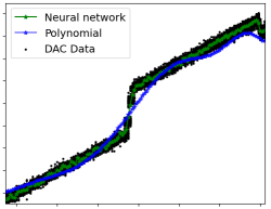
Figure 4: Polynomial vs. NN regression in the vicinity of a discontinuity for a CS-DAC behavioral model.

Note how the NN fits this region well while the polynomial exhibits both poor fitting near the discontinuity and oscillatory behavior. For this reason, we approach system identification using NN. The NN considered in this paper are feedforward MLP. An example of an MLP with a single hidden layer is shown in Figure 5, and the output $\hat{y}_{n}$ for this architecture with nonlinear activation $\underline{$h$}:\mathbb{R}^{H}\rightarrow\mathbb{R}^{H}$ is given by

$$\hat{y}_{n}={\bm{w}^{(1)}}^{\top}\,\underline{$h$}\left(\bm{w}^{(0)}\,x_{n}+\bm{b}^{(0)}\right)+b^{(1)}$$ (1)

where the set of trainable parameters $\theta$ is defined as

$$\theta:=\left\{\bm{w}^{(0)},\bm{w}^{(1)},\bm{b}^{(0)},b^{(1)}\right\}$$ (2)

with dimensions $\bm{w}^{(0)}\in\mathbb{R}^{H}$, $\bm{w}^{(1)}\in\mathbb{R}^{H}$, $\bm{b}^{(0)}\in\mathbb{R}^{H}$, $b^{(1)}\in\mathbb{R}$.

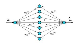
Figure 5: Single layer MLP with 1 input node, $H$ hidden nodes, and 1 output node.

III Simulation Results

In this section, dataset $\mathcal{D}_{\text{TRAIN}}$ is obtained using 10-bit DAC and ADC behavioral models operating at $f_{s}=40.96\text{GS/s}$. These MATLAB-based models accurately reflect the behavior of the DAC and ADC used in Section IV. We model the measurement path in Figure 3(a) as a $2^{\text{nd}}$ order Butterworth lowpass filter with 20GHz cutoff. The FFT of a two-tone waveform without any linearization is illustrated by the blue spectrum in Figure 6. Note that current source errors result in IM products, and the linearization objective is to suppress these as much as possible.

We approach system identification in a NN framework by minimizing the following MSE cost function

$$C_{\text{model}}=\frac{1}{N}\sum_{n=1}^{N}\left(\hat{y}_{n}-y_{n}\right)^{2}$$ (3)

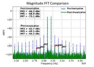
Figure 6: Two-tone FFT comparison before and after NN-based DPD. The signal frequencies are $f_{1}=3.1$GHz, $f_{2}=3.2$GHz with amplitudes -12dBFS/tone and the DAC is sampling at $f_{s}=40.96$GS/s.

by an appropriate selection of $\theta$, $H$, and $\underline{$h$}(\cdot)$. Conventionally, hyperparameters $H$, $\underline{$h$}(\cdot)$, and the number of hidden layers are chosen heuristically. However, in this paper, we leverage DnC, an automated framework for low complexity deep learning applications [10]. This results in single layer NN with ReLu activation [11] and $H=271$ hidden nodes. Model parameters $\theta$ are then obtained using an extended version of SGD [12], which completes system identification for the static transfer characteristic. The inverse of this transfer characteristic is then quantized to the 10-bit level and then stored in a LUT as shown in Figure 2.

The performance of NN-based DPD on the behavioral model is illustrated by the green spectrum in Figure 6, which shows a reduction of 23.6dB, 19.8dB, and 17.9dB for IM3, IM5, and IM7 respectively.

IV Measurement Results

In this section, we present results for NN-based DPD on a twofold time-interleaved 10-bit CS-DAC operating at $f_{s}=40.96$GS/s in 14nm CMOS. Our motivation is to demonstrate the ability to capture real-world nonlinearities and also avoid capturing dynamic properties of the system. We do not intend to compare the specific DAC used to state-of-the-art circuit research.

Dataset $\mathcal{D}_{\text{TRAIN}}$ is obtained by capturing the DAC output using an on-chip 10-bit ADC synchronized to the same sample rate as the DAC. The DAC is externally connected to the ADC to avoid undesired signal attenuation and filtering effects. The test setup is shown in Figure 7. Linearization was performed in the same NN framework described in Section III using a sine wave with frequency $f_{\text{sig}}$ = 100 MHz for system identification.

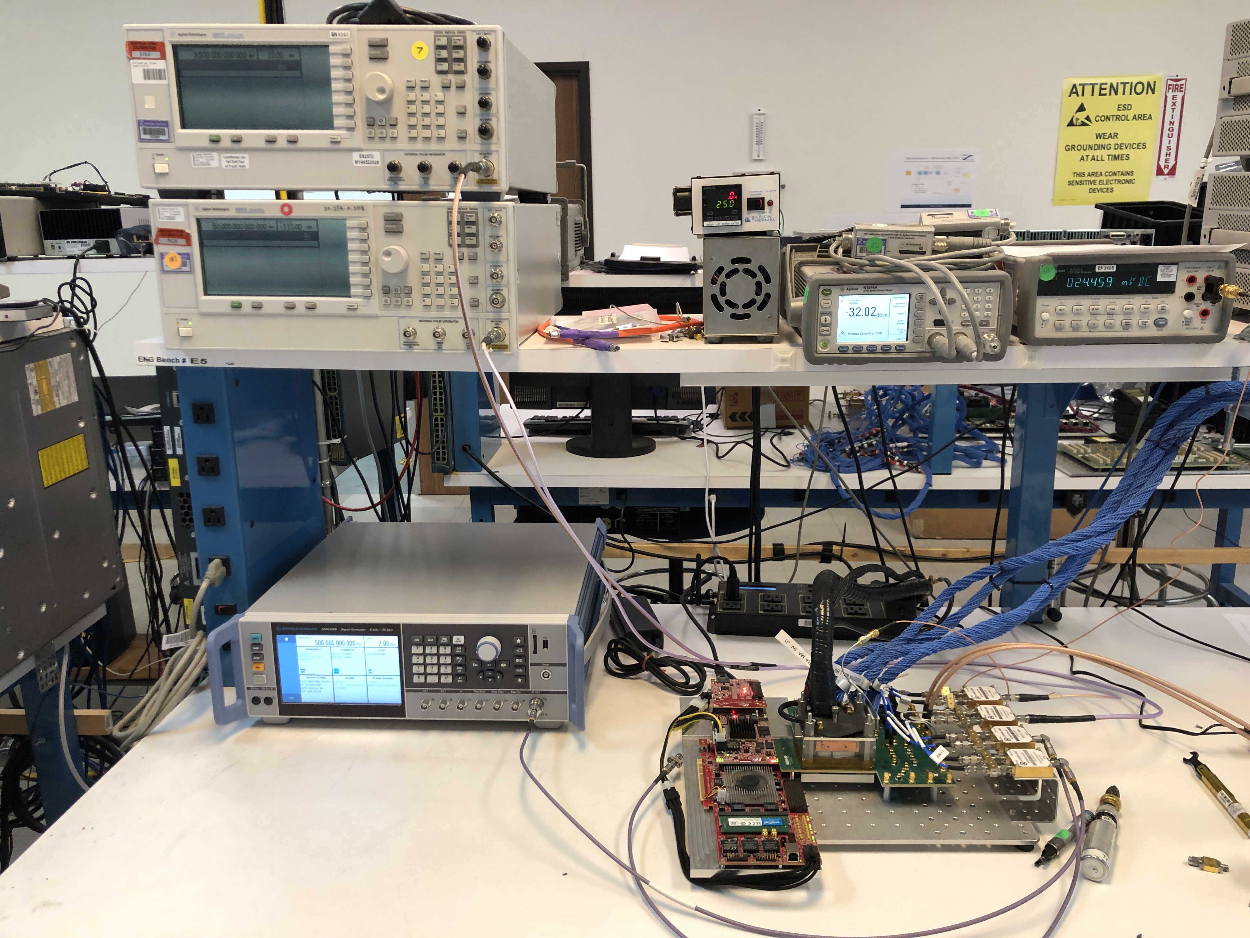
Figure 7: Test bench with the high-speed DAC and ADC test board.

The results are illustrated in Figure 8 and Figure 9, where we compare IM3/IM5/IM7 levels using two-tone signals centered at various frequencies across the first Nyquist zone. System identification is performed with amplitude -6dBFS, and performance is evaluated for both -6dBFS and -12dBFS. We compare the proposed NN technique with DEM and $15^{\text{th}}$ order polynomial-based DPD. An on-chip randomizer is used for the former, and coefficients for the latter are found by applying linear regression with a Vandermonde matrix.

Based on Figure 9, it is evident that NN-based DPD shows an improvement of at least 6dB for frequencies up to 9GHz for -12dBFS inputs. This is significant for sub-6GHz applications such as 5G. We suspect that pulse shape and timing errors begin to dominate linearity performance above 9GHz. Evidence for this is based on the efficacy of DEM above 9GHz, as it is proven to suppress such errors [13].

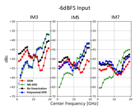
Figure 8: IM3/IM5/IM7 performance across Nyquist for two-tone signals, -12dBFS/tone (-6dBFS total amplitude), 100 MHz spacing.

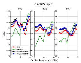
Figure 9: IM3/IM5/IM7 performance across Nyquist for two-tone signals, -18dBFS/tone (-12dBFS total amplitude), 100 MHz spacing.

V Conclusion

In this paper, we explored a novel linearization scheme for high-speed current steering DAC using NN. We showed that simple MLP are sufficient for system identification if low-frequency sine waves are used for training. The NN architecture is selected using DnC and parameters are found using SGD. The inverse of the transfer characteristic is then mapped onto the input codes using a LUT. The final implementation is a simple pre-distortion LUT with no NN required.

A useful extension would be to make this scheme adaptive with respect to temperature and supply voltage variation. This may be accomplished by using sensors coupled with multiple LUT. Lastly, our approach demonstrates an improvement of at least 6dB over conventional DEM and polynomial-based DPD methods for frequencies up to 9GHz.

References

- [1] W. Hong, Z. H. Jiang, C. Yu, J. Zhou, P. Chen, Z. Yu, H. Zhang, B. Yang, X. Pang, M. Jiang, Y. Cheng, M. K. T. Al-Nuaimi, Y. Zhang, J. Chen, and S. He, “Multibeam antenna technologies for 5G wireless communications,” IEEE Transactions on Antennas and Propagation, vol. 65, no. 12, pp. 6231–6249, 2017.
- [2] B. Ku, P. Schmalenberg, O. Inac, O. D. Gurbuz, J. S. Lee, K. Shiozaki, and G. M. Rebeiz, “A 77–81-GHz 16-element phased-array receiver with beam scanning for advanced automotive radars,” IEEE Transactions on Microwave Theory and Techniques, vol. 62, no. 11, pp. 2823–2832, 2014.
- [3] M. El-Chammas and B. Murmann, Time-Interleaved ADCs. New York, NY: Springer New York, 2012.
- [4] B. Razavi, “The current-steering DAC [a circuit for all seasons],” IEEE Solid-State Circuits Magazine, vol. 10, no. 1, pp. 11–15, 2018.
- [5] E. Olieman, Time-interleaved high-speed D/A converters, 2016.
- [6] D. Beauchamp and K. M. Chugg, “Machine learning based image calibration for a twofold time-interleaved high speed DAC,” in 2019 IEEE 62nd International Midwest Symposium on Circuits and Systems (MWSCAS), 2019, pp. 908–912.
- [7] C. Daigle, A. Dastgheib, and B. Murmann, “A 12-bit 800-MS/s switched-capacitor DAC with open-loop output driver and digital predistortion,” in 2010 IEEE Asian Solid-State Circuits Conference, 2010, pp. 1–4.
- [8] A. Dastgheib, “Calibration ADC and algorithm for adaptive predistortion of high-speed DACs,” Ph.D. dissertation, Stanford University, 2013.
- [9] A. Janczak, Identification of Nonlinear Systems Using Neural Networks and Polynomial Models: A Block-Oriented Approach (Lecture Notes in Control and Information Sciences). Berlin, Heidelberg: Springer-Verlag, 2004.
- [10] S. Dey, S. C. Kanala, K. M. Chugg, and P. A. Beerel, “Deep-n-Cheap: An automated search framework for low complexity deep learning,” arXiv e-print arXiv:2004.00974, 2020.
- [11] A. F. Agarap, “Deep learning using rectified linear units (relu),” arXiv preprint arXiv:1803.08375, 2018.
- [12] D. Kingma and J. Ba, “Adam: A method for stochastic optimization,” International Conference on Learning Representations, 12 2014.
- [13] K. L. Chan, J. Zhu, and I. Galton, “Dynamic element matching to prevent nonlinear distortion from pulse-shape mismatches in high-resolution DACs,” IEEE Journal of Solid-State Circuits, vol. 43, no. 9, pp. 2067–2078, 2008.