Landmark and IMU Data Fusion: Systematic Convergence Geometric Nonlinear Observer for SLAM and Velocity Bias

Abstract

Navigation solutions suitable for cases when both autonomous robot’s pose (i.e., attitude and position) and its environment are unknown are in great demand. Simultaneous Localization and Mapping (SLAM) fulfills this need by concurrently mapping the environment and observing robot’s pose with respect to the map. This work proposes a nonlinear observer for SLAM posed on the manifold of the Lie group of $\mathbb{SLAM}_{n}\left(3\right)$, characterized by systematic convergence, and designed to mimic the nonlinear motion dynamics of the true SLAM problem. The system error is constrained to start within a known large set and decay systematically to settle within a known small set. The proposed estimator is guaranteed to achieve predefined transient and steady-state performance and eliminate the unknown bias inevitably present in velocity measurements by directly using measurements of angular and translational velocity, landmarks, and information collected by an inertial measurement unit (IMU). Experimental results obtained by testing the proposed solution on a real-world dataset collected by a quadrotor demonstrate the observer’s ability to estimate the six-degrees-of-freedom (6 DoF) robot pose and to position unknown landmarks in three-dimensional (3D) space.

I Introduction

Robotic mapping and localization are fundamental navigation tasks. The nature of the problem is conditioned by the unknown component: robot’s pose, environment map or both. Simultaneous Localization and Mapping (SLAM) consists in concurrent mapping of the environment and identification of the robot’s pose (i.e, attitude and position). SLAM solutions are indispensable in absence of absolute positioning systems, such as global positioning systems (GPS), which are unsuitable for occluded environments. SLAM problem is generally tackled using a set of sensor measurements acquired at the body-fixed frame of the robot in motion. Owing to the presence of uncertain elements in the measurements, robust observers are an absolute necessity.

SLAM has been an active area of research over the past thirty years [1, 2, 3, 4, 5, 6, 7, 8, 9, 10]. Two traditional approaches to SLAM estimation are Gaussian filters and nonlinear observers. Variations of Gaussian filters for SLAM designed over the past decade include FastSLAM algorithm based on scalable approach [1], MonoSLAM algorithm on single camera [9], iSAM that considers fast incremental matrix factorization [11], extended Kalman filter (EKF) with consistency analysis [8, 12], invariant EKF [13], monocular visual-inertial state estimator [14], particle filter [15], and linear time-variant Kalman filter for visual SLAM [16]. The feature that unites all of the above-mentioned algorithms is the probabilistic framework. The three main challenges that characterize the SLAM estimation problem are: 1) the added complexity of robot motion in 3D space, 2) the duality of robot’s pose and map estimation, and above all 3) high nonlinearity of the problem. The true motion dynamics of SLAM consist of robot’s pose and landmark dynamics. Pose dynamics of a robot are framed on the Lie group of the special Euclidean group $\mathbb{SE}\left(3\right)$. Robot’s orientation, also referred to as attitude, is a fundamental part of landmark dynamics that belongs to the Special Orthogonal Group $\mathbb{SO}\left(3\right)$. Due to the fact that Gaussian filters fail to fully capture the true nonlinearity of the SLAM estimation problem, nonlinear observers are deemed more suitable.

Owing to the nonlinearity of the attitude and pose dynamics modeled on $\mathbb{SO}\left(3\right)$ and $\mathbb{SE}\left(3\right)$, respectively, over the past ten years several nonlinear observers have been developed on $\mathbb{SO}\left(3\right)$ [17, 18, 19] and $\mathbb{SE}\left(3\right)$ [20, 21, 22]. Consequently, nonlinear observers developed on $\mathbb{SE}\left(3\right)$ have been found suitable in application to the SLAM problem [23]. The duality and nonlinearity aspects of the SLAM problem have been tackled using a nonlinear observer for pose estimation and a Kalman filter for feature estimation [24]. However, the work in [24] did not fully capture the true nonlinearity of the SLAM problem. To address this shortcoming, a nonlinear observer for SLAM able to handle unknown bias attached to velocity measurements has been proposed in [5, 6]. Despite significant progress, none of the above-mentioned observers incorporated a measure that would guarantee error convergence for the transient and steady-state performance. Systematic convergence can be achieved and controlled by means of a prescribed performance function (PPF) [25]. PPF entails trapping the error to start within a predefined large set and reduce systematically and smoothly to stay among predefined small set [25, 26, 19, 27]. The error is constrained by dynamically reducing boundaries which is achieved by employing its unconstrained form termed transformed error.

It must be emphasized that the SLAM problem is nonlinear and is posed on the Lie group of $\mathbb{SLAM}_{n}\left(3\right)$. Taking into consideration the shortcomings of the previously proposed observers for SLAM, this work proposes a nonlinear observer that directly incorporates measurements of angular and translational velocities as well as landmark and IMU measurements distinguished by the following characteristics:

1. The nonlinear observer for SLAM is developed directly on the Lie group of $\mathbb{SLAM}_{n}\left(3\right)$ mimicking the true SLAM dynamics with guaranteed measures of transient and steady-state performance.

2. The error components of the Lyapunov function candidate have been proven to be asymptotically stable including the attitude error.

3. The proposed observer successfully compensates for the unknown bias in group velocity measurements.

Effectiveness and robustness of the proposed observer for six-degrees-of-freedom (6 DoF) robot pose estimation and mapping of the unknown landmarks in three-dimensional (3D) space have been confirmed experimentally using a real-world dataset collected by an unmanned aerial vehicle.

This paper consists of six sections: Section II provides a brief overview of mathematical notation and preliminaries, and defines the Lie group of $\mathbb{SO}\left(3\right)$, $\mathbb{SE}\left(3\right)$, and $\mathbb{SLAM}_{n}\left(3\right)$. Section III presents the true SLAM problem, the set of available measurements, and error criteria. Section IV presents the concept of PPF, mapping of the error to transformed error, and proposes the nonlinear observer for SLAM on $\mathbb{SLAM}_{n}\left(3\right)$. Section V presents the obtained results. Section VI summarizes the work.

II Preliminaries of $\mathbb{SLAM}_{n}\left(3\right)$

The sets of real numbers, nonnegative real numbers, $n$-dimensional Euclidean space, and $n$-by-$m$ dimensional space are denoted by $\mathbb{R}$, $\mathbb{R}_{+}$, $\mathbb{R}^{n}$, and $\mathbb{R}^{n\times m}$, respectively. $\left\|x\right\|=\sqrt{x^{\top}x}$ is an Euclidean norm for $x\in\mathbb{R}^{n}$. $\mathbf{I}_{n}$ and $\underline{\mathbf{0}}_{n}$ represent an $n$-dimensional identity matrix and a zero column vector, respectively. $\left\{\mathcal{I}\right\}$ represents an inertial-fixed-frame of reference, while $\left\{\mathcal{B}\right\}$ represents a body-fixed-frame. The Special Orthogonal Group $\mathbb{SO}\left(3\right)$ is defined by

$$\mathbb{SO}\left(3\right)=\left\{\left.R\in\mathbb{R}^{3\times 3}\right|RR^{\top}=R^{\top}R=\mathbf{I}_{3}\text{, }{\rm det}\left(R\right)=+1\right\}$$

where ${\rm det\left(\cdot\right)}$ refers to a determinant. Special Euclidean Group $\mathbb{SE}\left(3\right)$ is described by

$$\mathbb{SE}\left(3\right)=\left\{\left.\boldsymbol{T}=\left[\begin{array}[]{cc}R&P\\ \underline{\mathbf{0}}_{3}^{\top}&1\end{array}\right]\in\mathbb{R}^{4\times 4}\right|R\in\mathbb{SO}\left(3\right),P\in\mathbb{R}^{3}\right\}$$

where $P\in\mathbb{R}^{3}$ refers to position and $R\in\mathbb{SO}\left(3\right)$ refers to orientation, commonly termed attitude, which together constitute a homogeneous transformation matrix [20, 22]

$$\boldsymbol{T}=\mathcal{Z}(R,P)=\left[\begin{array}[]{cc}R&P\\ \underline{\mathbf{0}}_{3}^{\top}&1\end{array}\right]\in\mathbb{SE}\left(3\right)$$ (1)

that comprehensively describes the pose of a rigid-body in 3D space, with $\underline{\mathbf{0}}_{3}$ referring to a zero column vector. The Lie-algebra of $\mathbb{SO}\left(3\right)$ is

$$\mathfrak{so}\left(3\right)=\left\{\left.\left[\Omega\right]_{\times}\in\mathbb{R}^{3\times 3}\right|\left[\Omega\right]_{\times}^{\top}=-\left[\Omega\right]_{\times},\Omega\in\mathbb{R}^{3}\right\}$$

where $\left[\Omega\right]_{\times}$ is a skew symmetric matrix and the relevant map $\left[\cdot\right]_{\times}:\mathbb{R}^{3}\rightarrow\mathfrak{so}\left(3\right)$ is described by

$$\left[\Omega\right]_{\times}=\left[\begin{array}[]{ccc}0&-\Omega_{3}&\Omega_{2}\\ \Omega_{3}&0&-\Omega_{1}\\ -\Omega_{2}&\Omega_{1}&0\end{array}\right]\in\mathfrak{so}\left(3\right),\hskip 10.00002pt\Omega=\left[\begin{array}[]{c}\Omega_{1}\\ \Omega_{2}\\ \Omega_{3}\end{array}\right]$$

For $\Omega,V\in\mathbb{R}^{3}$ one has $\left[\Omega\right]_{\times}V=\Omega\times V$ where $\times$ signifies a cross product. $\mathfrak{se}\left(3\right)$ is the Lie-algebra of $\mathbb{SE}\left(3\right)$ described by

$$\mathfrak{se}\left(3\right)=\left\{\left[U\right]_{\wedge}\in\mathbb{R}^{4\times 4}\left|\exists\Omega,V\in\mathbb{R}^{3}:\left[U\right]_{\wedge}=\left[\begin{array}[]{cc}\left[\Omega\right]_{\times}&V\\ \underline{\mathbf{0}}_{3}^{\top}&0\end{array}\right]\right.\right\}$$

where $\left[\cdot\right]_{\wedge}$ refers to a wedge operator and the map $\left[\cdot\right]_{\wedge}:\mathbb{R}^{6}\rightarrow\mathfrak{se}\left(3\right)$ is described by

$$\left[U\right]_{\wedge}=\left[\begin{array}[]{cc}\left[\Omega\right]_{\times}&V\\ \underline{\mathbf{0}}_{3}^{\top}&0\end{array}\right]\in\mathfrak{se}\left(3\right),\hskip 10.00002ptU=\left[\begin{array}[]{c}\Omega\\ V\end{array}\right]\in\mathbb{R}^{6}$$

$\mathbf{vex}:\mathfrak{so}\left(3\right)\rightarrow\mathbb{R}^{3}$ describes the inverse mapping of $\left[\cdot\right]_{\times}$ such that

$$\begin{cases}\mathbf{vex}\left(\left[\Omega\right]_{\times}\right)&=\Omega,\hskip 10.00002pt\forall\Omega\in\mathbb{R}^{3}\\ \left[\mathbf{vex}(\left[\Omega\right]_{\times})\right]_{\times}&=\left[\Omega\right]_{\times}\in\mathfrak{so}\left(3\right)\end{cases}$$ (2)

$\boldsymbol{\mathcal{P}}_{a}$ denotes the anti-symmetric projection $\boldsymbol{\mathcal{P}}_{a}:\mathbb{R}^{3\times 3}\rightarrow\mathfrak{so}\left(3\right)$ where

$$\boldsymbol{\mathcal{P}}_{a}\left(X\right)=\frac{1}{2}(X-X^{\top})\in\mathfrak{so}\left(3\right),\hskip 10.00002pt\forall X\in\mathbb{R}^{3\times 3}$$ (3)

$\boldsymbol{\Upsilon}\left(\cdot\right)$ describes the composition mapping $\boldsymbol{\Upsilon}=\mathbf{vex}\circ\boldsymbol{\mathcal{P}}_{a}$ as

$$\boldsymbol{\Upsilon}\left(X\right)=\mathbf{vex}\left(\boldsymbol{\mathcal{P}}_{a}\left(X\right)\right)\in\mathbb{R}^{3},\hskip 10.00002pt\forall X\in\mathbb{R}^{3\times 3}$$ (4)

For $R\in\mathbb{SO}\left(3\right)$, $\left\|R\right\|_{{\rm I}}$ describes the Euclidean distance as

$$\left\|R\right\|_{{\rm I}}=\frac{1}{4}{\rm Tr}\{\mathbf{I}_{3}-R\}\in\left[0,1\right]$$ (5)

$\overset{\circ}{\mathcal{M}}$ and $\overline{\mathcal{M}}$ refer to submanifolds of $\mathbb{R}^{4}$ described by

$$\overset{\circ}{\mathcal{M}} =\left\{\left.\overset{\circ}{x}=\left[\begin{array}[]{cc}x^{\top}&0\end{array}\right]^{\top}\in\mathbb{R}^{4}\right|x\in\mathbb{R}^{3}\right\}$$

$$\overline{\mathcal{M}} =\left\{\left.\overline{x}=\left[\begin{array}[]{cc}x^{\top}&1\end{array}\right]^{\top}\in\mathbb{R}^{4}\right|x\in\mathbb{R}^{3}\right\}$$

Let $\mathbb{SLAM}_{n}\left(3\right)=\mathbb{SE}\left(3\right)\times\overline{\mathcal{M}}^{n}$ be a Lie group described by

$$\mathbb{SLAM}_{n}\left(3\right) =\left\{X=(\boldsymbol{T},\overline{{\rm p}})\left|\boldsymbol{T}\in\mathbb{SE}\left(3\right),\overline{{\rm p}}\in\overline{\mathcal{M}}^{n}\right.\right\}$$

$$\overline{{\rm p}} =[\overline{{\rm p}}_{1},\overline{{\rm p}}_{2},\ldots,\overline{{\rm p}}_{n}]\in\overline{\mathcal{M}}^{n}$$

$$\overline{\mathcal{M}}^{n} =\overline{\mathcal{M}}\times\overline{\mathcal{M}}\times\cdots\times\overline{\mathcal{M}}$$

where $\overline{{\rm p}}_{i}=\left[\begin{array}[]{cc}{\rm p}_{i}^{\top}&1\end{array}\right]^{\top}\in\overline{\mathcal{M}}$, for $i=1,2,\ldots,n$. $\mathfrak{slam}_{n}\left(3\right)=\mathfrak{se}\left(3\right)\times\overset{\circ}{\mathcal{M}}^{n}$ is the Lie algebra of $\mathbb{SLAM}_{n}\left(3\right)$, and the tangent space of the identity element is described by

$$\mathfrak{slam}_{n}\left(3\right) =\left\{\mathcal{Y}=(\left[U\right]_{\wedge},\overset{\circ}{{\rm v}})\left|\left[U\right]_{\wedge}\in\mathfrak{se}\left(3\right),\overset{\circ}{{\rm v}}\in\overset{\circ}{\mathcal{M}}^{n}\right.\right\}$$

$$\overset{\circ}{{\rm v}} =[\overset{\circ}{{\rm v}}_{1},\overset{\circ}{{\rm v}}_{2},\ldots,\overset{\circ}{{\rm v}}_{n}]\in\overset{\circ}{\mathcal{M}}^{n}$$

$$\overset{\circ}{\mathcal{M}}^{n} =\overset{\circ}{\mathcal{M}}\times\overset{\circ}{\mathcal{M}}\times\cdots\times\overset{\circ}{\mathcal{M}}$$

where $\overset{\circ}{{\rm v}}_{i}=\left[\begin{array}[]{cc}{\rm v}_{i}^{\top}&0\end{array}\right]^{\top}\in\overset{\circ}{\mathcal{M}}$, for $i=1,2,\ldots,n$. The identities below will be used in the forthcoming derivations

$$\left[a\times b\right]_{\times}= ba^{\top}-ab^{\top},\hskip 10.00002ptb,a\in{\rm\mathbb{R}}^{3}$$ (6)

$$\left[Ra\right]_{\times}= R\left[b\right]_{\times}R^{\top},\hskip 10.00002pta\in{\rm\mathbb{R}}^{3},R\in\mathbb{SO}\left(3\right)$$ (7)

$${\rm Tr}\left\{M\left[a\right]_{\times}\right\}= {\rm Tr}\left\{\boldsymbol{\mathcal{P}}_{a}\left(M\right)\left[a\right]_{\times}\right\},\hskip 10.00002pta\in{\rm\mathbb{R}}^{3},M\in\mathbb{R}^{3\times 3}$$

$$= -2\mathbf{vex}\left(\boldsymbol{\mathcal{P}}_{a}\left(M\right)\right)^{\top}a$$ (8)

III SLAM Problem

III-A Available Measurements

Suppose that the map contains $n$ landmarks as illustrated in Fig. 1. Let $R\in\mathbb{SO}\left(3\right)$, $P\in\mathbb{R}^{3}$, and ${\rm p}_{i}\in\mathbb{R}^{3}$ be rigid-body’s orientation, rigid-body’s translation, and the $i$th landmark location in 3D space, respectively, where $R\in\left\{\mathcal{B}\right\}$, $P\in\left\{\mathcal{I}\right\}$, and ${\rm p}_{i}\in\left\{\mathcal{I}\right\}$ for all $i=1,2,\ldots,n$. SLAM problem considers a completely unknown environment, and therefore, involves simultaneous estimation of 1) robot’s pose $\boldsymbol{T}\in\mathbb{SE}\left(3\right)$ (position and orientation), and 2) landmark positions $\overline{{\rm p}}=[\overline{{\rm p}}_{1},\overline{{\rm p}}_{2},\ldots,\overline{{\rm p}}_{n}]\in\overline{\mathcal{M}}^{n}$ with the aid of a set of measurements. Fig. 1 presents a schematic depiction of the SLAM estimation problem.

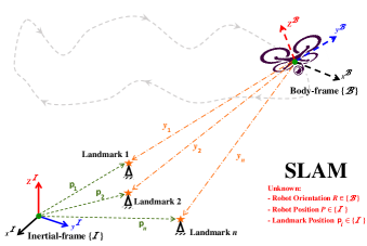
Figure 1: Graphical illustration of SLAM estimation problem.

From (1), define $X=(\boldsymbol{T},\overline{{\rm p}})\in\mathbb{SLAM}_{n}\left(3\right)$ as an unknown combination of the true rigid-body’s pose and the true landmark positions. Define $\mathcal{Y}=[\left[U\right]_{\wedge},\overset{\circ}{{\rm v}}]\in\mathfrak{slam}_{n}\left(3\right)$ as the true group velocity where $\overset{\circ}{{\rm v}}=[\overset{\circ}{{\rm v}}_{1},\overset{\circ}{{\rm v}}_{2},\ldots,\overset{\circ}{{\rm v}}_{n}]\in\overset{\circ}{\mathcal{M}}^{n}$ and $U,\overset{\circ}{{\rm v}}\in\left\{\mathcal{B}\right\}$. Note that the available measurement $\mathcal{Y}$ is assumed to be both continuous and bounded. Define $U=\left[\Omega^{\top},V^{\top}\right]^{\top}\in\mathbb{R}^{6}$ as a group velocity vector expressed relative to the body-frame, with $\Omega\in\mathbb{R}^{3}$ and $V\in\mathbb{R}^{3}$ describing the true angular and translational velocity, respectively, and ${\rm v}_{i}\in\mathbb{R}^{3}$ describing the $i$th linear velocity of the $i$th landmark with respect to the body-frame for all $\Omega,V,{\rm v}_{i}\in\left\{\mathcal{B}\right\}$. This paper concerns fixed landmarks, signifying that $\dot{{\rm p}}_{i}=\underline{\mathbf{0}}_{3}$, and therefore, linear velocity of a landmark expressed in the body-frame as ${\rm v}_{i}=\underline{\mathbf{0}}_{3}$ $\forall i=1,2,\ldots,n$. The measurements of angular and translational velocities $U_{m}=\left[\Omega_{m}^{\top},V_{m}^{\top}\right]^{\top}\in\mathbb{R}^{6}$ are defined by

$$\begin{cases}\Omega_{m}&=\Omega+b_{\Omega}\in\mathbb{R}^{3}\\ V_{m}&=V+b_{V}\in\mathbb{R}^{3}\end{cases}$$ (9)

with $b_{\Omega}$ and $b_{V}$ being unknown constant bias attached to the measurements of $\Omega$ and $V$, respectively. Let us define $b_{U}=\left[b_{\Omega}^{\top},b_{V}^{\top}\right]^{\top}\in\mathbb{R}^{6}$ for all $U_{m},b_{U}\in\left\{\mathcal{B}\right\}$. The body-frame vectors relevant to the orientation determination $\overset{\circ}{a}_{j}=[a_{j}^{\top},0]^{\top}$ are described by [18, 19]

$$\overset{\circ}{a}_{j}=\boldsymbol{T}^{-1}\overset{\circ}{r}_{j}+\overset{\circ}{b}_{j}^{a}+\overset{\circ}{n}_{j}^{a}\in\overset{\circ}{\mathcal{M}},\hskip 10.00002ptj=1,2,\ldots,n_{R}$$ (10)

where $\overset{\circ}{r}_{j}=[r_{j}^{\top},0]^{\top}\in\left\{\mathcal{I}\right\}$, $\overset{\circ}{b}_{j}^{a}=[b_{j}^{a^{\top}},0]^{\top}\in\left\{\mathcal{B}\right\}$, and $\overset{\circ}{n}_{j}^{a}=[n_{j}^{a^{\top}},0]^{\top}\in\left\{\mathcal{B}\right\}$ describe the $j$th known inertial-frame observation, unknown constant bias, and unknown random noise, respectively. Also, $\boldsymbol{T}^{-1}=\mathcal{Z}(R^{\top},-R^{\top}P)$ and let $b_{j}^{a}=n_{j}^{a}=0$. Note that (10) exemplifies measurements obtained from a low cost IMU. Both $r_{j}$ and $a_{j}$ in (10) can be normalized as shown in (11) and employed to establish the orientation

$$\upsilon_{j}^{r}=\frac{r_{j}}{\left\|r_{j}\right\|},\hskip 10.00002pt\upsilon_{j}^{a}=\frac{a_{j}}{\left\|a_{j}\right\|}$$ (11)

Remark 1.

[18, 19] The rigid-body’s orientation can be established given the availability of three non-collinear vectors for both $\upsilon_{j}^{r}$ and $\upsilon_{j}^{a}$. If $n_{R}=2$, the third vector can be defined through $\upsilon_{3}^{a}=\upsilon_{1}^{a}\times\upsilon_{2}^{a}$ and $\upsilon_{3}^{r}=\upsilon_{1}^{r}\times\upsilon_{2}^{r}$, respectively.

Given an environment with $n$ landmarks, the $i$th landmark measurement in the body-frame $\overline{y}_{i}=[y_{i}^{\top},1]^{\top}$can be described by

$$\overline{y}_{i}=\boldsymbol{T}^{-1}\overline{{\rm p}}_{i}+\overset{\circ}{b}_{i}^{y}+\overset{\circ}{n}_{i}^{y}\in\overline{\mathcal{M}},\hskip 10.00002pt\forall i=1,2,\ldots,n$$ (12)

with $\overset{\circ}{b}_{i}^{y}\in\overset{\circ}{\mathcal{M}}$ and $\overset{\circ}{n}_{i}^{y}\in\overset{\circ}{\mathcal{M}}$ describing unknown constant bias and random noise, respectively.

Assumption 1.

[20, 22] It is assumed that the total number of landmarks available for measurement is three or more.

III-B True SLAM Kinematics and Error Criteria

The true SLAM dynamics in (13) are $X=(\boldsymbol{T},\overline{{\rm p}})\in\mathbb{SLAM}_{n}\left(3\right)$, and the tangent space of $X$ is $\mathcal{Y}=(\left[U\right]_{\wedge},\overset{\circ}{{\rm v}})\in\mathfrak{slam}_{n}\left(3\right)$ defined by

$$\begin{cases}\dot{\boldsymbol{T}}&=\boldsymbol{T}\left[U\right]_{\wedge}\\ \dot{{\rm p}}_{i}&=R{\rm v}_{i},\hskip 10.00002pt\forall i=1,2,\ldots,n\end{cases}$$ (13)

which can be represented in a simplified form as

$$\begin{cases}\dot{R}&=R\left[\Omega\right]_{\times}\\ \dot{P}&=RV\\ \dot{{\rm p}}_{i}&=R{\rm v}_{i},\hskip 10.00002pt\forall i=1,2,\ldots,n\end{cases}$$

where $U=\left[\Omega^{\top},V^{\top}\right]^{\top}$ describes the true group velocity vector and ${\rm v}_{i}\in\mathbb{R}^{3}$ describes the $i$th linear velocity of ${\rm p}_{i}$ with respect to the body-frame. Define the estimate of pose as

$$\hat{\boldsymbol{T}}=\mathcal{Z}(\hat{R},\hat{P})=\left[\begin{array}[]{cc}\hat{R}&\hat{P}\\ \underline{\mathbf{0}}_{3}^{\top}&1\end{array}\right]\in\mathbb{SE}\left(3\right)$$

where $\hat{R}$ represents the estimate of true orientation and $\hat{P}$ stands for the estimate of the true position. Let $\hat{{\rm p}}_{i}$ be the estimate of the true $i$th landmark ${\rm p}_{i}$. Define error between $\boldsymbol{T}$ and $\hat{\boldsymbol{T}}$ by

$$\tilde{\boldsymbol{T}}=\hat{\boldsymbol{T}}\boldsymbol{T}^{-1} =\left[\begin{array}[]{cc}\hat{R}&\hat{P}\\ \underline{\mathbf{0}}_{3}^{\top}&1\end{array}\right]\left[\begin{array}[]{cc}R^{\top}&-R^{\top}P\\ \underline{\mathbf{0}}_{3}^{\top}&1\end{array}\right]$$ (18)

$$=\left[\begin{array}[]{cc}\tilde{R}&\tilde{P}\\ \underline{\mathbf{0}}_{3}^{\top}&1\end{array}\right]=\mathcal{Z}(\tilde{R},\tilde{P})$$ (21)

where $\tilde{R}=\hat{R}R^{\top}$ denotes the orientation error and $\tilde{P}=\hat{P}-\tilde{R}P$ describes the position error. The ultimate goal of pose estimation is to asymptotically drive $\tilde{\boldsymbol{T}}\rightarrow\mathbf{I}_{4}$ and, consequently, drive $\tilde{R}\rightarrow\mathbf{I}_{3}$ and $\tilde{P}\rightarrow\underline{\mathbf{0}}_{3}$. As such, let the error between $\hat{{\rm p}}_{i}$ and ${\rm p}_{i}$ be defined as

$$\overset{\circ}{e}_{i}=\overline{\hat{{\rm p}}}_{i}-\tilde{\boldsymbol{T}}\,\overline{{\rm p}}_{i}$$ (22)

such that $\overline{\hat{{\rm p}}}_{i}=\left[\hat{{\rm p}}_{i}^{\top},1\right]^{\top}\in\overline{\mathcal{M}}$ and $\overset{\circ}{e}_{i}=\left[e_{i}^{\top},0\right]^{\top}\in\overset{\circ}{\mathcal{M}}$. Based on the definition of $\tilde{\boldsymbol{T}}$ in (21), $\overset{\circ}{e}_{i}=\overline{\hat{{\rm p}}}_{i}-\hat{\boldsymbol{T}}\boldsymbol{T}^{-1}\,\overline{{\rm p}}_{i}$ and, in view of (12), one has

$$\overset{\circ}{e}_{i}=\overline{\hat{{\rm p}}}_{i}-\hat{\boldsymbol{T}}\,\overline{y}_{i}$$ (23)

The error in (12) is represented with respect to the estimates and vector measurements. Hence, it can be found that $\overset{\circ}{e}_{i}=\left[\tilde{{\rm p}}_{i}^{\top}-\tilde{P}^{\top},0\right]^{\top}$where $\tilde{{\rm p}}_{i}=\hat{{\rm p}}_{i}-\tilde{R}{\rm p}_{i}$ describes the error of the $i$th landmark estimate and $\tilde{P}=\hat{P}-\tilde{R}P$ as defined in (21).

III-C IMU Setup

This work proposes an observer design directly dependent on a group of measurements. As a result, it is essential to formulate a group of variables in terms of vector measurements. According to the vectorial body-frame measurements in (10) and the related normalization in (11), define

$$M=M^{\top}=\sum_{j=1}^{n_{{\rm R}}}s_{j}\upsilon_{j}^{r}\left(\upsilon_{j}^{r}\right)^{\top},\hskip 10.00002pt\forall j=1,2,\ldots n_{{\rm R}}$$ (24)

with $s_{j}\geq 0$ being a constant gain describes the confidence level of the $j$th sensor measurement. It is evident that $M$ is symmetric. According to Remark 1, it is assumed that $n_{{\rm R}}\geq 2$ such that no less than two non-collinear body-frame measurements and inertial-frame observations are available. Consequently, ${\rm rank}(M)=3$. Describe the eigenvalues of $M$ as $\lambda_{1}$, $\lambda_{2}$, and $\lambda_{3}$. Thus, all of $\lambda_{1}$, $\lambda_{2}$, and $\lambda_{3}$ are positive. Define a new variable $\breve{\mathbf{M}}={\rm Tr}\left\{M\right\}\mathbf{I}_{3}-M$ provided that ${\rm rank}(M)=3$. As a result, ${\rm rank}(\breve{\mathbf{M}})=3$ and [28]:

1. $\breve{\mathbf{M}}$ is positive-definite.

2. The three eigenvalues of $\breve{\mathbf{M}}$ are $\lambda_{2}+\lambda_{3}$, $\lambda_{3}+\lambda_{1}$, and $\lambda_{2}+\lambda_{1}$, and $\underline{\lambda}(\breve{\mathbf{M}})>0$.

where $\underline{\lambda}(\cdot)$ denotes the minimum eigenvalue of a matrix. In the remainder of the paper it is considered that ${\rm rank}\left(M\right)=3$ and $s_{j}$ is selected such that $\sum_{j=1}^{n_{{\rm R}}}s_{j}=3$ for $j=1,2,\ldots n_{{\rm R}}$. This in turn implies that ${\rm Tr}\left\{M\right\}=3$.

Lemma 1.

Let $\tilde{R}\in\mathbb{SO}\left(3\right)$, $M=M^{\top}\in\mathbb{R}^{3\times 3}$ as in (24) with ${\rm Tr}\{M\}=3$ and ${\rm rank}\{M\}=3$. Define $\breve{\mathbf{M}}={\rm Tr}\{M\}\mathbf{I}_{3}-M$ with $\underline{\lambda}=\underline{\lambda}(\breve{\mathbf{M}})$ being its minimum singular value. Then, the following holds

$$||\tilde{R}M||_{{\rm I}} \leq\frac{2}{\underline{\lambda}}\frac{||\mathbf{vex}(\boldsymbol{\mathcal{P}}_{a}(\tilde{R}M))||^{2}}{1+{\rm Tr}\{\tilde{R}MM^{-1}\}}$$ (25)

Proof. See the Appendix in [19].

Definition 1.

Define a non-attractive and forward invariant unstable set $\mathcal{U}_{s}\subseteq\mathbb{SO}\left(3\right)$ as

$$\mathcal{U}_{s}=\left\{\left.\tilde{R}\left(0\right)\in\mathbb{SO}\left(3\right)\right|{\rm Tr}\{\tilde{R}\left(0\right)\}=-1\right\}$$ (26)

$\tilde{R}\left(0\right)\in\mathcal{U}_{s}$ is possible given one of the following three scenarios: $\tilde{R}\left(0\right)={\rm diag}(1,-1,-1)$, $\tilde{R}\left(0\right)={\rm diag}(-1,1,-1)$, and $\tilde{R}\left(0\right)={\rm diag}(-1,-1,1)$.

The expressions in (10) and (11) entail that the true normalized value of the $j$th body-frame vector is defined by $\upsilon_{j}^{a}=R^{\top}\upsilon_{j}^{r}$. Hence, define the estimate of the body-frame vector as

$$\hat{\upsilon}_{j}^{a}=\hat{R}^{\top}\upsilon_{j}^{r},\hskip 10.00002pt\forall j=1,2,\ldots n_{{\rm R}}$$ (27)

Define the error in pose as in (21) where $\tilde{R}=\hat{R}R^{\top}$. By the virtue of the identities in (7) and (6), one has

$$\left[\hat{R}\sum_{j=1}^{n_{{\rm R}}}\frac{s_{j}}{2}\hat{\upsilon}_{j}^{a}\times\upsilon_{j}^{a}\right]_{\times} =\hat{R}\sum_{j=1}^{n_{{\rm R}}}\frac{s_{j}}{2}\left(\upsilon_{j}^{a}\left(\hat{\upsilon}_{j}^{a}\right)^{\top}-\hat{\upsilon}_{j}^{a}\left(\upsilon_{j}^{a}\right)^{\top}\right)\hat{R}^{\top}$$

$$=\frac{1}{2}\hat{R}R^{\top}M-\frac{1}{2}MR\hat{R}^{\top}$$

$$=\boldsymbol{\mathcal{P}}_{a}(\tilde{R}M)$$

If follows that $\mathbf{vex}(\boldsymbol{\mathcal{P}}_{a}(\tilde{R}M))$ with respect to vector measurements is as below

$$\boldsymbol{\Upsilon}(\tilde{R}M)=\mathbf{vex}(\boldsymbol{\mathcal{P}}_{a}(\tilde{R}M))=\hat{R}\sum_{j=1}^{n_{{\rm R}}}(\frac{s_{j}}{2}\hat{\upsilon}_{j}^{a}\times\upsilon_{j}^{a})$$ (28)

Moreover, $\tilde{R}M$ can be specified in terms of vector measurements as

$$\tilde{R}M=\hat{R}\sum_{j=1}^{n_{{\rm R}}}\left(s_{j}\upsilon_{j}^{a}\left(\upsilon_{j}^{r}\right)^{\top}\right)$$ (29)

Note that ${\rm Tr}\left\{M\right\}=3$, and, according to the definition in (5), the normalized Euclidean distance of $\tilde{R}M$ in terms of vector measurements is

$$e_{\tilde{R}}=||\tilde{R}M||_{{\rm I}} =\frac{1}{4}{\rm Tr}\{(\mathbf{I}_{3}-\tilde{R})M\}$$

$$=\frac{1}{4}{\rm Tr}\left\{\mathbf{I}_{3}-\hat{R}\sum_{j=1}^{n_{{\rm R}}}\left(s_{j}\upsilon_{j}^{a}\left(\upsilon_{j}^{r}\right)^{\top}\right)\right\}$$

$$=\frac{1}{4}\sum_{j=1}^{n_{{\rm R}}}\left(1-s_{j}\left(\hat{\upsilon}_{j}^{a}\right)^{\top}\upsilon_{j}^{a}\right)$$ (30)

Also, from (5), one has

$$1-||\tilde{R}||_{{\rm I}} =1-\frac{1}{4}{\rm Tr}\{\mathbf{I}_{3}-\tilde{R}\}=\frac{1}{4}(1+{\rm Tr}\{\tilde{R}\})$$ (31)

Accordingly, from (31), one obtains

$$1-||\tilde{R}||_{{\rm I}} =\frac{1}{4}(1+{\rm Tr}\{\tilde{R}MM^{-1}\})$$ (32)

From (32) and (29), one finds

$$\pi(\tilde{R},M)={\rm Tr}\{\tilde{R}MM^{-1}\}$$

$$\hskip 3.00003pt={\rm Tr}\left\{\left(\sum_{j=1}^{n_{{\rm R}}}s_{j}\upsilon_{j}^{a}\left(\upsilon_{j}^{r}\right)^{\top}\right)\left(\sum_{j=1}^{n_{{\rm R}}}s_{j}\hat{\upsilon}_{j}^{a}\left(\upsilon_{j}^{r}\right)^{\top}\right)^{-1}\right\}$$ (33)

With the aim of making the observer design adaptive, consider the estimate of the unknown bias $b_{U}$ to be $\hat{b}_{U}=\left[\hat{b}_{\Omega}^{\top},\hat{b}_{V}^{\top}\right]^{\top}$. Define the error between $b_{U}$ and $\hat{b}_{U}$ as

$$\begin{cases}\tilde{b}_{\Omega}&=b_{\Omega}-\hat{b}_{\Omega}\\ \tilde{b}_{V}&=b_{V}-\hat{b}_{V}\end{cases}$$ (34)

where $\tilde{b}_{U}=\left[b_{\Omega}^{\top},\tilde{b}_{V}^{\top}\right]^{\top}\in\mathbb{R}^{6}$. Prior to proceeding, it is crucial to incorporate the nonlinearity of the true SLAM problem into the proposed observer design. Thus, the proposed observer follows $\hat{X}=(\hat{\boldsymbol{T}},\overline{\hat{{\rm p}}})\in\mathbb{SLAM}_{n}\left(3\right)$ and its tangent space is $\hat{\mathcal{Y}}=([\hat{U}]_{\wedge},\overset{\circ}{\hat{{\rm v}}})\in\mathfrak{slam}_{n}\left(3\right)$ where $\hat{\boldsymbol{T}}\in\mathbb{SE}\left(3\right)$, $\overline{\hat{{\rm p}}}=[\overline{\hat{{\rm p}}}_{1},\ldots,\overline{\hat{{\rm p}}}_{n}]\in\overline{\mathcal{M}}^{n}$, $\hat{U}\in\mathfrak{se}\left(3\right)$, and $\overset{\circ}{\hat{{\rm v}}}=[\overset{\circ}{\hat{{\rm v}}}_{1},\ldots,\overset{\circ}{\hat{{\rm v}}}_{n}]\in\overset{\circ}{\mathcal{M}}^{n}$ are the estimates of pose, landmark positions, group velocity, and linear landmark velocity, respectively.

IV Nonlinear Observer Design with Systematic Convergence

This section presents the nonlinear observer design for SLAM with guaranteed transient and steady-state performance. The nonlinear observer design is based on the measurements obtained from an IMU and the landmarks within the environment.

IV-A Systematic Convergence

Recall the error in the normalized Euclidean distance $e_{\tilde{R}}$ defined in (30) and the landmark estimation $e_{i}=[e_{i,1},e_{i,2},e_{i,3}]^{\top}$ defined in (23). This subsection aims to reformulate the SLAM estimation problem such that $e_{\tilde{R}}$ and $e_{i}$ follow the predefined transient and steady-state properties adjusted by the user. The key objective of the reformulation consists in using predefined reducing boundaries to fully control the process of error initiation within a given large set and its continuous decay towards a given small set. This can be achieved via prescribed performance functions (PPF) [25] defined as positive, time-decreasing, and smooth functions $\xi_{i,k}:\mathbb{R}_{+}\to\mathbb{R}_{+}$ and $\xi_{\tilde{R}}:\mathbb{R}_{+}\to\mathbb{R}_{+}$ such that

$$\begin{cases}\xi_{i,k}\left(t\right)&=(\xi_{i,k}^{0}-\xi_{i,k}^{\infty})\exp(-\ell_{i,k}t)+\xi_{i,k}^{\infty}\\ \xi_{\tilde{R}}\left(t\right)&=(\xi_{\tilde{R}}^{0}-\xi_{\tilde{R}}^{\infty})\exp(-\ell_{\tilde{R}}t)+\xi_{\tilde{R}}^{\infty}\end{cases}$$ (35)

where $\xi_{i}=[\xi_{i,1},\xi_{i,2},\xi_{i,3}]^{\top}\in\mathbb{R}^{3}$, $\xi_{\tilde{R}}\left(0\right)=\xi_{\tilde{R}}^{0}$ and $\xi_{i}\left(0\right)=\xi_{i}^{0}=[\xi_{i,1}^{0},\xi_{i,2}^{0},\xi_{i,3}^{0}]^{\top}\in\mathbb{R}^{3}$ represent the initial value and the upper bound of $\xi_{\tilde{R}}$ and $\xi_{i}$, respectively. $\xi_{\tilde{R}}^{\infty}$ and $\xi_{i}^{\infty}=[\xi_{i,1}^{\infty},\xi_{i,2}^{\infty},\xi_{i,3}^{\infty}]^{\top}\in\mathbb{R}^{3}$ correspond to the upper bound of the small sets, $\ell_{\tilde{R}}$ and $\ell_{i}=[\ell_{i,1},\ell_{i,2},\ell_{i,3}]^{\top}\in\mathbb{R}^{3}$ signify positive constants that control the rate of convergence of $\xi_{\tilde{R}}\left(t\right)$ and $\xi\left(t\right)$, respectively, for all $i=1,2,\ldots,n$, and $k=1,2,3$. For simplicity, let the subscript $\star$ denote the appropriate component $\tilde{R}$ or $i,k$. This way, $e_{\star}\left(t\right)$ is guaranteed to obey the predefined dynamically reducing boundaries, if one of the following conditions is fulfilled:

$$-\delta_{\star}\xi_{\star}\left(t\right)<e_{\star}\left(t\right)<\xi_{\star}\left(t\right), \text{ if }e_{\star}\left(0\right)\geq 0$$ (36)

$$-\xi_{\star}\left(t\right)<e_{\star}\left(t\right)<\delta_{\star}\xi_{\star}\left(t\right), \text{ if }e_{\star}\left(0\right)<0$$ (37)

with $\delta_{\star}\in\left[0,1\right]$. Define $e_{\star}:=e_{\star}\left(t\right)$ and $\xi_{\star}:=\xi_{\star}\left(t\right)$. The systematic convergence of $e_{\star}$ from a known large set to a known narrow set defined in (36) and (37) is presented in Fig. 2.

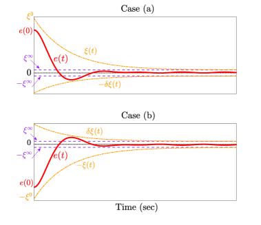
Figure 2: Systematic convergence of $e_{\star}$ with respect to (a) Equation (36); (b) Equation (37).

Remark 2.

[25, 19, 20, 29, 30] Note that specifying the upper bound as well as the sign of $e_{\star}\left(0\right)$ is sufficient to compel the error to adhere to the performance constraints and obey the predefined dynamically reducing boundaries $\forall t>0$. Given that one of the conditions in (36) and (37) is met, the maximum undershoot/overshoot will be bounded by $\pm\delta\xi_{\star}$ and the steady-state error will be limited by $\pm\xi_{\star}^{\infty}$as detailed in Fig. 2.

Let the error $e_{\star}$ be given as

$$e_{\star}=\xi_{\star}\mathcal{F}(E_{\star})$$ (38)

where $\xi_{\star}\in\mathbb{R}$ is as expressed in (35), $E_{\star}\in\mathbb{R}$ represents the unconstrained error known as transformed error, and $\mathcal{F}(E_{\star})$ represents a smooth function and follows Assumption 2:

Assumption 2.

The smooth function $\mathcal{F}(E_{\star})$ has the following characteristics [25, 19, 20]:

1. $\mathcal{F}(E_{\star})$ strictly increasing.

2. $\mathcal{F}(E_{\star})$ is constrained by
   $-\underline{\delta}_{\star}<\mathcal{F}(E_{\star})<\bar{\delta}_{\star},{\rm\text{ if }}e_{\star}\left(0\right)\geq 0$
   $-\bar{\delta}_{\star}<\mathcal{F}(E_{\star})<\underline{\delta}_{\star},{\rm\text{ if }}e_{\star}\left(0\right)<0$
   where $\bar{\delta}_{\star}$ and $\underline{\delta}_{\star}$ are positive constants with $\underline{\delta}_{\star}\leq\bar{\delta}_{\star}$.

4. $\left.\begin{array}[]{c}\underset{E_{\star}\rightarrow-\infty}{\lim}\mathcal{F}(E_{\star})=-\underline{\delta}_{\star}\\ \underset{E_{\star}\rightarrow+\infty}{\lim}\mathcal{F}(E_{\star})=\bar{\delta}_{\star}\end{array}\right\}{\rm\text{ if }}e_{\star}\left(0\right)\geq 0$
   $\left.\begin{array}[]{c}\underset{E_{\star}\rightarrow-\infty}{\lim}\mathcal{F}(E_{\star})=-\bar{\delta}_{\star}\\ \underset{E_{\star}\rightarrow+\infty}{\lim}\mathcal{F}(E_{\star})=\underline{\delta}_{\star}\end{array}\right\}{\rm\text{ if }}e_{\star}\left(0\right)<0$
   such that

$$\mathcal{F}\left(E_{\star}\right)=\begin{cases}\frac{\bar{\delta}_{\star}\exp(E_{\star})-\underline{\delta}_{\star}\exp(-E_{\star})}{\exp(E_{\star})+\exp(-E_{\star})},&\bar{\delta}_{\star}\geq\underline{\delta}_{\star}\text{ if }e_{\star}\left(0\right)\geq 0\\ \frac{\bar{\delta}_{\star}\exp(E_{\star})-\underline{\delta}_{\star}\exp(-E_{\star})}{\exp(E_{\star})+\exp(-E_{\star})},&\underline{\delta}_{\star}\geq\bar{\delta}_{\star}\text{ if }e_{\star}\left(0\right)<0\end{cases}$$ (39)

$E_{\star}$ can be expressed via inverse transformation of (39)

$$E_{\star}(e_{\star},\xi_{\star})=\mathcal{F}^{-1}(e_{\star}/\xi_{\star})$$ (40)

In view of (39), the inverse transformation of $\mathcal{F}\left(E_{\star}\right)$ is given by

$$E_{\star}= \frac{1}{2}\begin{cases}\text{ln}\frac{\underline{\delta}_{\star}+e_{\star}/\xi_{\star}}{\bar{\delta}_{\star}-e_{\star}/\xi_{\star}},&\bar{\delta}_{\star}\geq\underline{\delta}_{\star}\text{ if }e_{\star}\left(0\right)\geq 0\\ \text{ln}\frac{\underline{\delta}_{\star}+e_{\star}/\xi_{\star}}{\bar{\delta}_{\star}-e_{\star}/\xi_{\star}},&\underline{\delta}_{\star}\geq\bar{\delta}_{\star}\text{ if }e_{\star}\left(0\right)<0\end{cases}$$ (41)

Proposition 1.

Consider $e_{\tilde{R}}$ in (30) and $e_{i,k}$ in (23). Recall (38), (39), and (40), and let the transformed error of $E_{\tilde{R}}$ and $E_{i,k}$ be described as in (41) given that $\underline{\delta}_{\tilde{R}}=\bar{\delta}_{\tilde{R}}$ and $\underline{\delta}_{i,k}=\bar{\delta}_{i,k}$. Then, the following holds:

1. The only possible representation of $E_{\tilde{R}}$ is

   $$E_{\tilde{R}}=\frac{1}{2}\text{ln}\frac{\bar{\delta}_{\tilde{R}}+e_{\tilde{R}}/\xi_{\tilde{R}}}{\underline{\delta}_{\tilde{R}}-e_{\tilde{R}}/\xi_{\tilde{R}}}$$ (42)

2. The transformed error $E_{\tilde{R}}>0\forall e_{\tilde{R}}\neq 0$ and $E_{i,k}\neq 0\forall e_{i,k}\neq 0$.

3. $E_{\star}=0$ only at $e_{\star}=0$.

Proof.

Due to the fact that $e_{\tilde{R}}=||\tilde{R}M||_{{\rm I}}=\frac{1}{4}{\rm Tr}\{(\mathbf{I}_{3}-\tilde{R})M\}$ and $M$ is positive definite, $e_{\tilde{R}}>0\forall\tilde{R}\neq\mathbf{I}_{3}$ and $e_{\tilde{R}}=0$ only at $\tilde{R}=\mathbf{I}_{3}$. As such, the upper portion of (41) holds $\forall t\geq 0$ which proves (i). Since Proposition 1 states that $\underline{\delta}_{\tilde{R}}=\bar{\delta}_{\tilde{R}}$ and $\underline{\delta}_{i,k}=\bar{\delta}_{i,k}$ with the constraint of $e_{\tilde{R}}\leq\xi_{\tilde{R}}$ and $e_{i,k}\leq\xi_{i,k}$, the expression in (42) is $(\bar{\delta}_{\tilde{R}}+e_{\tilde{R}}/\xi_{\tilde{R}})/(\underline{\delta}_{\tilde{R}}-e_{\tilde{R}}/\xi_{\tilde{R}})\geq 1\forall e_{\tilde{R}}\neq 0$ and $(\bar{\delta}_{i,k}+e_{i,k}/\xi_{i,k})/(\underline{\delta}_{i,k}-e_{i,k}/\xi_{i,k})\neq 1\forall e_{i,k}\neq 0$. Moreover, it logically follows that at $e_{\star}=0$, $E_{\star}=\frac{1}{2}\text{ln}(\bar{\delta}_{\star}/\underline{\delta}_{\star})=0$. This proves (ii) and (iii).∎

Consider

$$\Lambda_{\star} =\frac{1}{2\xi_{\star}}\frac{\partial\mathcal{F}^{-1}(e_{\star}/\xi_{\star})}{\partial(e_{\star}/\xi_{\star})}$$

$$=\frac{1}{2\xi_{\star}}(\frac{1}{\underline{\delta}_{\star}+e_{\star}/\xi_{\star}}+\frac{1}{\bar{\delta}_{\star}-e_{\star}/\xi_{\star}})$$

Define the following variables

$$\begin{cases}\mu_{\tilde{R}}&=\dot{\xi}_{\tilde{R}}/\xi_{\tilde{R}}\\ \mu_{i}&={\rm diag}\left(\dot{\xi}_{i,1}/\xi_{i,1},\dot{\xi}_{i,2}/\xi_{i,2},\dot{\xi}_{i,3}/\xi_{i,3}\right)\\ \Lambda_{i}&={\rm diag}(\Lambda_{i,1},\Lambda_{i,2},\Lambda_{i,3})\end{cases}$$ (43)

for $i=1,2,\ldots,n$. Thus, one finds that the transformed error dynamics of $E_{\tilde{R}}$ and $E_{i}=\left[E_{i,1},E_{i,2},E_{i,3}\right]^{\top}$ are as follows:

$$\begin{cases}\dot{E}_{\tilde{R}}&=\Lambda_{\tilde{R}}(\dot{e}_{\tilde{R}}-\mu_{\tilde{R}}e_{\tilde{R}})\\ \dot{E}_{i}&=\Lambda_{i}(\dot{e}_{i}-\mu_{i}e_{i})\end{cases}$$ (44)

IV-B Nonlinear Observer Design

Consider the following nonlinear observer

$$\begin{cases}\dot{\hat{\boldsymbol{T}}}&=\hat{\boldsymbol{T}}\left[U_{m}-\hat{b}_{U}-W_{U}\right]_{\wedge}\\ \dot{{\rm\hat{p}}}_{i}&=-k_{1}\Lambda_{i}E_{i}+\hat{R}\left[y_{i}\right]_{\times}W_{\Omega},\hskip 10.00002pti=1,2,\ldots,n\\ \dot{\hat{b}}_{\Omega}&=\frac{\Lambda_{\tilde{R}}}{2}\Gamma_{1}\hat{R}^{\top}\boldsymbol{\Upsilon}(\tilde{R}M)-\sum_{i=1}^{n}\frac{\Gamma_{2}}{\alpha_{i}}\left[y_{i}\right]_{\times}\hat{R}^{\top}\Lambda_{i}E_{i}\\ \dot{\hat{b}}_{V}&=-\sum_{i=1}^{n}\frac{\Gamma_{2}}{\alpha_{i}}\hat{R}^{\top}\Lambda_{i}E_{i}\\ \tau_{R}&=\underline{\lambda}(\breve{\mathbf{M}})\times\left(1+\pi(\tilde{R},M)\right)\\ W_{\Omega}&=\frac{k_{w}\Lambda_{\tilde{R}}-4\mu_{\tilde{R}}}{\tau_{R}}\hat{R}^{\top}\boldsymbol{\Upsilon}(\tilde{R}M)\\ W_{V}&=-\sum_{i=1}^{n}\frac{1}{\alpha_{i}}k_{2}\hat{R}^{\top}\Lambda_{i}E_{i}\end{cases}$$ (45)

where $W_{U}=\left[W_{\Omega}^{\top},W_{V}^{\top}\right]^{\top}\in\mathbb{R}^{6}$ is a correction factor and $\hat{b}_{U}$ is an estimate of $b_{U}$. $k_{1}$, $k_{2}$, $k_{w}$, $\Gamma=\left[\begin{array}[]{cc}\Gamma_{1}&0_{3\times 3}\\ 0_{3\times 3}&\Gamma_{2}\end{array}\right]$, and $\alpha_{i}$ denote positive constants. Note that $M$, $\pi(\tilde{R},M)$, $\boldsymbol{\Upsilon}(\tilde{R}M)$, and $e_{i}$ are defined with respect to the available measurements in (24), (33), (28), and (23), respectively, for all $i=1,2,\ldots,n$.

Theorem 1.

Consider the SLAM kinematics $\dot{X}=(\dot{\boldsymbol{T}},\dot{\overline{{\rm p}}})$ in (13) in combination with the measurements extracted from landmarks ($\overline{y}_{i}=\boldsymbol{T}^{-1}\overline{{\rm p}}_{i}$), inertial measurement units $\upsilon_{j}^{a}=R^{\top}\upsilon_{j}^{r}$, and velocity measurements ($U_{m}=U+b_{U}$) for all $i=1,2,\ldots,n$ and $j=1,2,\ldots n_{{\rm R}}$. Let Assumption 1 hold and the observer design be as in (45), supplied with the measurements $U_{m}$, $\upsilon_{j}^{a}$ and $\overline{y}_{i}$. Let the design parameters $\xi_{\star}^{0}\geq e_{\star}\left(0\right)$, $\underline{\delta}_{\star}=\bar{\delta}_{\star}$, $k_{1}$, $k_{2}$, $k_{w}$, $\Gamma$, and $\alpha_{i}$ be selected as positive constants. Define the following set:

$$\mathcal{S}= \left\{\left(E_{\tilde{R}},E_{1},E_{2},\ldots,E_{n}\right)\in\mathbb{R}\times\mathbb{R}^{3}\times\mathbb{R}^{3}\times\cdots\times\mathbb{R}^{3}\right|$$

$$\hskip 50.00008pt\left.E_{\tilde{R}}=0,E_{i}=\underline{\mathbf{0}}_{3}\forall i=1,2,\ldots n\right\}$$ (46)

with $E_{\tilde{R}}\left(0\right)\in\mathcal{L}_{\infty}$, $E_{i}\left(0\right)\in\mathcal{L}_{\infty}$ and $\tilde{R}\left(0\right)\notin\mathcal{U}_{s}$. Then, 1) all signals in the closed loop are bounded, 2) the error $(E_{\tilde{R}},E_{1},E_{2},\ldots,E_{n})$ asymptotically approaches $\mathcal{S}$, 3) the error $(e_{\tilde{R}},e_{1},e_{2},\ldots,e_{n})$ asymptotically approaches the origin, 4) $\tilde{R}$ asymptotically approaches the attractive equilibrium point $\mathbf{I}_{3}$, and 5) $\tilde{b}_{U}$ asymptotically approaches the origin.

Proof.

In order to prove Theorem 1, it is necessary to derive transformed error dynamics $\dot{E}_{\star}=\dot{E}_{\star}(e_{\star},\dot{e}_{\star})$ in (44). It becomes evident that $\dot{E}_{\star}$ is a function of the pose and the landmark error as well as the error dynamics. As such, the first step is to find the pose and landmark error dynamics. Recall the pose error $\tilde{\boldsymbol{T}}$ defined in (21). Thus, the pose error dynamics are

$$\dot{\tilde{\boldsymbol{T}}} =\dot{\hat{\boldsymbol{T}}}\boldsymbol{T}^{-1}+\hat{\boldsymbol{T}}\dot{\boldsymbol{T}}^{-1}$$

$$=\hat{\boldsymbol{T}}\left[U+\tilde{b}_{U}-W_{U}\right]_{\wedge}\boldsymbol{T}^{-1}-\hat{\boldsymbol{T}}\left[U\right]_{\wedge}\boldsymbol{T}^{-1}$$

$$=\hat{\boldsymbol{T}}\left[\tilde{b}_{U}-W_{U}\right]_{\wedge}\hat{\boldsymbol{T}}^{-1}\tilde{\boldsymbol{T}}$$ (47)

where $\boldsymbol{\dot{T}}^{-1}=-\boldsymbol{T}^{-1}\boldsymbol{\dot{T}}\boldsymbol{T}^{-1}$. Thereby, the error dynamics of $\overset{\circ}{e}_{i}$ in (22) become

$$\overset{\circ}{\dot{e}}_{i} =\overset{\circ}{\dot{\hat{{\rm p}}}}_{i}-\dot{\tilde{\boldsymbol{T}}}\,\overline{{\rm p}}_{i}-\tilde{\boldsymbol{T}}\,\dot{\overline{{\rm p}}}_{i}$$

$$=\overset{\circ}{\dot{\hat{{\rm p}}}}_{i}-\hat{\boldsymbol{T}}\left[\tilde{b}_{U}-W_{U}\right]_{\wedge}\hat{\boldsymbol{T}}^{-1}\tilde{\boldsymbol{T}}\,\overline{{\rm p}}_{i}$$ (48)

The expression $\hat{\boldsymbol{T}}\left[\tilde{b}_{U}\right]_{\wedge}\hat{\boldsymbol{T}}^{-1}$ in (47) can be reformulated as

$$\hat{\boldsymbol{T}}\left[\tilde{b}_{U}\right]_{\wedge}\hat{\boldsymbol{T}}^{-1} =\left[\begin{array}[]{cc}\hat{R}[\tilde{b}_{\Omega}]_{\times}\hat{R}^{\top}&\hat{R}\tilde{b}_{V}-\hat{R}[\tilde{b}_{\Omega}]_{\times}\hat{R}^{\top}\hat{P}\\ \underline{\mathbf{0}}_{3}^{\top}&0\end{array}\right]$$ (51)

$$=\left[\begin{array}[]{c}\hat{R}\tilde{b}_{\Omega}\\ \hat{R}\tilde{b}_{V}+[\hat{P}]_{\times}\hat{R}\tilde{b}_{\Omega}\end{array}\right]_{\wedge}\in\mathfrak{se}\left(3\right)$$ (54)

with $[\hat{R}\tilde{b}_{\Omega}]_{\times}=\hat{R}[\tilde{b}_{\Omega}]_{\times}\hat{R}^{\top}$ as defined in (7), which shows that the expression in (54) is equivalent to

$$\hat{\boldsymbol{T}}\left[\tilde{b}_{U}\right]_{\wedge}\hat{\boldsymbol{T}}^{-1}=\left[\left[\begin{array}[]{cc}\hat{R}&0_{3\times 3}\\ \left[\hat{P}\right]_{\times}\hat{R}&\hat{R}\end{array}\right]\tilde{b}_{U}\right]_{\wedge}$$ (55)

Hence, in view of (55) and (48), one obtains

$$\hat{\boldsymbol{T}}\left[\tilde{b}_{U}\right]_{\wedge}\hat{\boldsymbol{T}}^{-1}\tilde{\boldsymbol{T}}\,\overline{{\rm p}}_{i} =\left[\left[\begin{array}[]{cc}\hat{R}&0_{3\times 3}\\ \left[\hat{P}\right]_{\times}\hat{R}&\hat{R}\end{array}\right]\tilde{b}_{U}\right]_{\wedge}\left[\begin{array}[]{c}\hat{R}y_{i}+\hat{P}\\ 1\end{array}\right]$$ (60)

$$=\left[\begin{array}[]{c}-\left[\hat{R}y_{i}\right]_{\times}\hat{R}\tilde{b}_{\Omega}+\hat{R}\tilde{b}_{V}\\ 0\end{array}\right]$$ (63)

$$=\left[\begin{array}[]{cc}-\hat{R}\left[y_{i}\right]_{\times}&\hat{R}\\ \underline{\mathbf{0}}_{3}^{\top}&\underline{\mathbf{0}}_{3}^{\top}\end{array}\right]\tilde{b}_{U}$$ (66)

From (48) and (66), the error dynamics in (48) become

$$\overset{\circ}{\dot{e}}_{i} =\overset{\circ}{\dot{\hat{{\rm p}}}}_{i}-\left[\begin{array}[]{cc}-\hat{R}\left[y_{i}\right]_{\times}&\hat{R}\\ \underline{\mathbf{0}}_{3}^{\top}&\underline{\mathbf{0}}_{3}^{\top}\end{array}\right]\left(\tilde{b}_{U}-W_{U}\right)$$ (69)

Note that the last row of (69) is comprised of zeros which means that

$$\dot{e}_{i} =\dot{\hat{{\rm p}}}_{i}-[\begin{array}[]{cc}-\hat{R}\left[y_{i}\right]_{\times}&\hat{R}\end{array}](\tilde{b}_{U}-W_{U})$$ (71)

From (47), the attitude error dynamics are

$$\dot{\tilde{R}} =\dot{\hat{R}}R^{\top}+\hat{R}\dot{R}^{\top}=\hat{R}\left[\tilde{b}_{\Omega}-W_{\Omega}\right]_{\times}R^{\top}$$

$$=\left[\hat{R}(\tilde{b}_{\Omega}-W_{\Omega})\right]_{\times}\tilde{R}$$ (72)

where the identity in (7) was utilized. In view of (5), $e_{\tilde{R}}=\frac{1}{4}{\rm Tr}\left\{(\mathbf{I}_{3}-\tilde{R})M\right\}$. As such, with the aid of (8) one has

$$\dot{e}_{\tilde{R}}= -\frac{1}{4}{\rm Tr}\left\{\left[\hat{R}(\tilde{b}_{\Omega}-W_{\Omega})\right]_{\times}\tilde{R}M\right\}$$

$$= -\frac{1}{4}{\rm Tr}\left\{\tilde{R}M\boldsymbol{\mathcal{P}}_{a}\left(\left[\hat{R}(\tilde{b}_{\Omega}-W_{\Omega})\right]_{\times}\right)\right\}$$

$$= \frac{1}{2}\mathbf{vex}\left(\boldsymbol{\mathcal{P}}_{a}(\tilde{R}M)\right)^{\top}\hat{R}(\tilde{b}_{\Omega}-W_{\Omega})$$ (73)

To this end, from (71) and (73), the transformed error dynamics can be represented as

$$\begin{cases}\dot{E}_{\tilde{R}}&=\Lambda_{\tilde{R}}\left(\frac{1}{2}\boldsymbol{\Upsilon}(\tilde{R}M)^{\top}\hat{R}(\tilde{b}_{\Omega}-W_{\Omega})-\mu_{\tilde{R}}e_{\tilde{R}}\right)\\ \dot{E}_{i}&=\Lambda_{i}\left(\dot{\hat{{\rm p}}}_{i}-[\begin{array}[]{cc}-\hat{R}\left[y_{i}\right]_{\times}&\hat{R}\end{array}](\tilde{b}_{U}-W_{U})-\mu_{i}e_{i}\right)\end{cases}$$ (74)

Note that $\mu_{\tilde{R}}$ and $\mu_{i}$ are vanishing components, and therefore, $\mu_{\tilde{R}},\mu_{i}\rightarrow 0$ as $t\rightarrow\infty$. Define the following candidate Lyapunov function $V=V(E_{\tilde{R}},E_{1},E_{2},\ldots,E_{n},\tilde{b}_{U})$

$$V=E_{\tilde{R}}+\sum_{i=1}^{n}\frac{1}{4\alpha_{i}}\left\|E_{i}\right\|^{2}+\frac{1}{2}\tilde{b}_{U}^{\top}\Gamma^{-1}\tilde{b}_{U}$$ (75)

From (74) and (75), the time derivative of $V$ is

$$\dot{V}=\dot{E}_{\tilde{R}}+\sum_{i=1}^{n}\frac{1}{\alpha_{i}}E_{i}^{\top}\dot{E}_{i}-\tilde{b}_{U}^{\top}\Gamma^{-1}\dot{\hat{b}}_{U}$$

$$=\sum_{i=1}^{n}\frac{1}{\alpha_{i}}\left[\begin{array}[]{c}\Lambda_{\tilde{R}}\boldsymbol{\Upsilon}(\tilde{R}M)\\ \Lambda_{i}E_{i}\end{array}\right]^{\top}\left[\begin{array}[]{cc}\frac{\alpha_{i}}{2}\hat{R}&0_{3\times 3}\\ \hat{R}[y_{i}]_{\times}&-\hat{R}\end{array}\right](\tilde{b}_{U}-W_{U})$$ (80)

$$\hskip 5.0pt+\sum_{i=1}^{n}\frac{1}{\alpha_{i}}E_{i}^{\top}\Lambda_{i}\left(\dot{\hat{{\rm p}}}_{i}-\mu_{i}e_{i}\right)-\Lambda_{\tilde{R}}\mu_{\tilde{R}}e_{\tilde{R}}-\tilde{b}_{U}^{\top}\Gamma^{-1}\dot{\hat{b}}_{U}$$ (81)

By (38) and (41) $|e_{i,k}|\leq\mu_{i,k}\bar{\delta}_{i,k}\xi_{i,k}|E_{i,k}|$, and moreover, $\mu_{i,k}$ is a vanishing component. Replacing $W_{U}$, $\dot{\hat{b}}_{U}$, and $\dot{\hat{{\rm p}}}_{i}$ with their definition in (45), one has

$$\dot{V}= -\sum_{i=1}^{n}\frac{k_{1}}{\alpha_{i}}\left\|\Lambda_{i}E_{i}\right\|^{2}-\frac{k_{w}\Lambda_{\tilde{R}}^{2}}{2\tau_{R}}\left\|\boldsymbol{\Upsilon}(\tilde{R}M)\right\|^{2}$$

$$-k_{2}\left\|\sum_{i=1}^{n}\frac{1}{\alpha_{i}}\Lambda_{i}E_{i}\right\|^{2}$$ (82)

In view of the result of Lemma 1, $2||\boldsymbol{\Upsilon}(\tilde{R}M)||^{2}/\tau_{R}\geq e_{\tilde{R}}$. Also, from (39), $e_{\tilde{R}}=\xi_{\tilde{R}}\frac{\bar{\delta}_{\tilde{R}}\exp(E_{\tilde{R}})-\underline{\delta}_{\tilde{R}}\exp(-E_{\tilde{R}})}{\exp(E_{\tilde{R}})+\exp(-E_{\tilde{R}})}$. Hence, the expression in (82) becomes

$$\dot{V}\leq -\frac{k_{w}}{8}\Lambda_{\tilde{R}}^{2}\xi_{\tilde{R}}\frac{\bar{\delta}_{\tilde{R}}\exp(E_{\tilde{R}})-\underline{\delta}_{\tilde{R}}\exp(-E_{\tilde{R}})}{\exp(E_{\tilde{R}})+\exp(-E_{\tilde{R}})}$$

$$-\sum_{i=1}^{n}\frac{k_{1}}{\alpha_{i}}\left\|\Lambda_{i}E_{i}\right\|^{2}-k_{2}\left\|\sum_{i=1}^{n}\frac{1}{\alpha_{i}}\Lambda_{i}E_{i}\right\|^{2}$$ (83)

From (83), given that $E_{\tilde{R}}\left(0\right)\in\mathcal{L}_{\infty}$, $E_{i}\left(0\right)\in\mathcal{L}_{\infty}$, and $\tilde{R}\left(0\right)\notin\mathcal{U}_{s}$, $\dot{V}<0$ for all $E_{i}\neq\underline{\mathbf{0}}_{3}$ or $E_{\tilde{R}}\neq 0$, and $\dot{V}=0$ only at $E_{i}=\underline{\mathbf{0}}_{3}$ and $E_{\tilde{R}}=0$ for all $i=1,2,\ldots,n$. Accordingly, the inequality in (83) ensures that $E_{i}$ and $E_{\tilde{R}}$ asymptotically converge to the set $\mathcal{S}$ in (46). Also, $\dot{V}$ is negative, continuous, and $\dot{V}\rightarrow 0$ such that $V\in\mathcal{L}_{\infty}$ and a finite $\lim_{t\rightarrow\infty}V$ exists. According to (iii) in Proposition 1, $E_{i}\neq\underline{\mathbf{0}}_{3}$ for $e_{i}\neq 0$, $E_{\tilde{R}}\neq 0$ for $e_{\tilde{R}}\neq 0$, $E_{i}=\underline{\mathbf{0}}_{3}$ only at $e_{i}=0$, while $E_{\tilde{R}}=0$ only at $e_{\tilde{R}}=0$, respectively. Thus, $e_{i}\rightarrow 0$ and $e_{\tilde{R}}=||\tilde{R}M||_{{\rm I}}\rightarrow 0$ as $t\rightarrow\infty$. Note that $e_{\tilde{R}}\rightarrow 0$ implies that $\tilde{R}\rightarrow\mathbf{I}_{3}$. By (25) in Lemma 1, $e_{\tilde{R}}\rightarrow 0$ strictly indicates that $\boldsymbol{\Upsilon}(\tilde{R}M)\rightarrow\underline{\mathbf{0}}_{3}$. Thus, from (45), $W_{U}\rightarrow 0$ as $E_{i}\rightarrow\underline{\mathbf{0}}_{3}$ and $\boldsymbol{\Upsilon}(\tilde{R}M)\rightarrow\underline{\mathbf{0}}_{3}$. Recall $\tilde{b}_{U}$ and $\dot{\hat{b}}_{U}$ in (34) and (45). $\dot{\tilde{b}}_{U}=-\dot{\hat{b}}_{U}$ implies that $\dot{\tilde{b}}_{U}\rightarrow 0$ as $E_{i}\rightarrow\underline{\mathbf{0}}_{3}$ and $\boldsymbol{\Upsilon}(\tilde{R}M)\rightarrow\underline{\mathbf{0}}_{3}$. As such, $\tilde{b}_{U}$ is bounded for all $t\geq 0$. In addition, from (45), $\dot{{\rm\hat{p}}}_{i}\rightarrow 0$ as $E_{i}\rightarrow 0$ and $W_{U}\rightarrow 0$. In accordance with the aforementioned discussion and based on the fact that $\lim_{t\rightarrow\infty}\dot{e}_{i}=0$, one obtains

$$\lim_{t\rightarrow\infty}\dot{e}_{i}=\lim_{t\rightarrow\infty}-[\begin{array}[]{cc}-\hat{R}\left[y_{i}\right]_{\times}&\hat{R}\end{array}]\tilde{b}_{U}=0$$

Algorithm 1 Systematic convergence nonlinear observer for SLAM

Initialization:

1. Set $\hat{R}\left(0\right)\in\mathbb{SO}\left(3\right)$ and $\hat{P}\left(0\right)\in\mathbb{R}^{3}$. As an alternative, construct $\hat{R}\left(0\right)\in\mathbb{SO}\left(3\right)$ using one of the attitude determination methods in [31]

2. Set ${\rm\hat{p}}_{i}\left(0\right)\in\mathbb{R}^{3}$ for all $i=1,2,\ldots,n$

3. Set $\hat{b}_{\Omega}\left(0\right)=\hat{b}_{V}\left(0\right)=0_{3\times 1}$

4. Select $\xi_{\star}^{0}$, $\xi_{\star}^{\infty}$, $\ell_{\star}$, $\bar{\delta}_{\star}=\underline{\delta}_{\star}$, $k_{w}$, $k_{1}$, $k_{2}$, $\Gamma$, and $\alpha_{i}$ as positive constants

while                  $\forall i=1,2,\ldots,n,\text{ and }j=1,2,\ldots n_{{\rm R}}$

1. Recall measurements and observations in (10) and their normalization $\upsilon_{j}^{r}=\frac{r_{j}}{\left\|r_{j}\right\|},\upsilon_{j}^{a}=\frac{a_{j}}{\left\|a_{j}\right\|}$ in (11)

2. $\hat{\upsilon}_{j}^{a}=\hat{R}^{\top}\upsilon_{j}^{r}$ as in (27)

3. $M=\sum_{j=1}^{n_{{\rm R}}}s_{j}\upsilon_{j}^{r}\left(\upsilon_{j}^{r}\right)^{\top}$ as in (24) with $\breve{\mathbf{M}}={\rm Tr}\left\{M\right\}\mathbf{I}_{3}-M$

4. $\boldsymbol{\Upsilon}=\hat{R}\sum_{j=1}^{n_{{\rm R}}}\left(\frac{s_{j}}{2}\hat{\upsilon}_{j}^{a}\times\upsilon_{j}^{a}\right)$ as in (28)

5. $\pi={\rm Tr}\left\{\left(\sum_{j=1}^{n_{{\rm R}}}s_{j}\upsilon_{j}^{a}\left(\upsilon_{j}^{r}\right)^{\top}\right)\left(\sum_{j=1}^{n_{{\rm R}}}s_{j}\hat{\upsilon}_{j}^{a}\left(\upsilon_{j}^{r}\right)^{\top}\right)^{-1}\right\}$ as in (33)

6. $e_{i}=\hat{{\rm p}}_{i}-\hat{R}y_{i}-\hat{P}$ as in (23)

7. $\xi_{\star}=\left(\xi_{\star}^{0}-\xi_{\star}^{\infty}\right)\exp(-\ell_{\star}t)+\xi_{\star}^{\infty}$ as in (35) and $\Lambda_{\star}$ as in (43)

8. $E_{\star}=\frac{1}{2}\text{ln}\frac{\bar{\delta}_{\star}+e_{\star}/\xi_{\star}}{\underline{\delta}_{\star}-e_{\star}/\xi_{\star}}$ as in (41)

9. $W_{\Omega}=\frac{k_{w}\Lambda_{\tilde{R}}-4\mu_{\tilde{R}}}{\tau_{R}}\hat{R}^{\top}\boldsymbol{\Upsilon}$, with $\tau_{R}=\underline{\lambda}(\breve{\mathbf{M}})\times(1+\pi[k])$

10. $W_{V}=-\sum_{i=1}^{n}\frac{k_{2}}{\alpha_{i}}\hat{R}^{\top}\Lambda_{i}E_{i}$

11. $\dot{\hat{R}}=\hat{R}\left[\Omega_{m}-\hat{b}_{\Omega}-W_{\Omega}\right]_{\times}$

12. $\dot{\hat{P}}=\hat{R}(V_{m}-\hat{b}_{V}-W_{V})$

13. $\dot{\hat{b}}_{\Omega}=\frac{\Gamma_{1}}{2}\hat{R}^{\top}\Lambda_{\tilde{R}}\boldsymbol{\Upsilon}-\sum_{i=1}^{n}\frac{\Gamma_{2}}{\alpha_{i}}\left[y_{i}\right]_{\times}\hat{R}^{\top}\Lambda_{i}E_{i}$

14. $\dot{\hat{b}}_{V}=-\sum_{i=1}^{n}\frac{\Gamma_{2}}{\alpha_{i}}\hat{R}^{\top}\Lambda_{i}E_{i}$

15. $\dot{{\rm\hat{p}}}_{i}=-k_{1}\Lambda_{i}E_{i}+\hat{R}\left[y_{i}\right]_{\times}W_{\Omega}$

end while

Consistently with Assumption 1, define

$$Q=-\left[\begin{array}[]{cc}-\hat{R}[y_{1}]_{\times}&\hat{R}\\ \vdots&\vdots\\ -\hat{R}[y_{n}]_{\times}&\hat{R}\end{array}\right]\in\mathbb{R}^{3n\times 6},\hskip 10.00002ptn\geq 3$$

Hence, $Q$ is full column rank such that $\lim_{t\rightarrow\infty}Q\tilde{b}_{U}=0$ results in $\lim_{t\rightarrow\infty}\tilde{b}_{U}=0$. Therefore, $\ddot{V}$ is bounded. On the grounds of Barbalat Lemma, $\dot{V}$ is uniformly continuous. According to the fact that $\tilde{b}_{U}\rightarrow 0$ and $W_{U}\rightarrow 0$ as $t\rightarrow\infty$, $\dot{\tilde{\boldsymbol{T}}}\rightarrow 0$, and in turn, $\tilde{\boldsymbol{T}}\rightarrow\boldsymbol{T}_{c}(\mathbf{I}_{3},P_{c})$, where $\boldsymbol{T}_{c}(\mathbf{I}_{3},P_{c})\in\mathbb{SE}\left(3\right)$ is a constant matrix with $P_{c}\in\mathbb{R}^{3}$ describing a constant vector. Consequently, $\lim_{t\rightarrow\infty}\tilde{P}=P_{c}$ completing the proof.∎

The complete implementation steps are described in Algorithm 1.

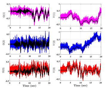
Figure 3: Angular and translational velocities: True vs measurements with extra additive noise.

V Experimental Results

In this section, the performance of the proposed nonlinear SLAM observer developed on the Lie group $\mathbb{SLAM}_{n}\left(3\right)$ and characterized by systematic convergence is tested and evaluated. The observing capabilities and robustness of the proposed approach against noise are demonstrated using a real-world EuRoc dataset [32]. The dataset includes 1) ground truth data that consists of the unmanned aerial vehicle true flight trajectory, 2) IMU measurements, and 3) stereo images. Due to the lack of real-world landmarks in the dataset, a set of virtual landmarks defined in the previous section is utilized. According to the dataset, the true attitude and position of the robot in 3D space are initialized at

$$P\left(0\right) =[-1.0761,0.4925,1.3299]^{\top},$$

$$R\left(0\right) =\left[\begin{array}[]{ccc}-0.2645&-0.0014&-0.9644\\ 0.0198&0.9998&-0.0069\\ 0.9642&-0.0210&-0.2645\end{array}\right]\in\mathbb{SO}\left(3\right)$$

Consider four inertial-frame-fixed landmarks placed at ${\rm p}_{1}=[2,0,0]^{\top}$, ${\rm p}_{2}=[-2,0,0]^{\top}$, ${\rm p}_{3}=[0,2,0]^{\top}$, and ${\rm p}_{4}=[0,-2,0]^{\top}$. The initial estimates of the robot attitude and position in 3D are as follows:

$$\hat{P}\left(0\right) =[0,0,0]^{\top},$$

$$\hat{R}\left(0\right) =\left[\begin{array}[]{ccc}-0.2653&-0.0642&-0.9620\\ 0.0032&0.9977&-0.0675\\ 0.9642&-0.0210&-0.2645\end{array}\right]\in\mathbb{SO}\left(3\right)$$

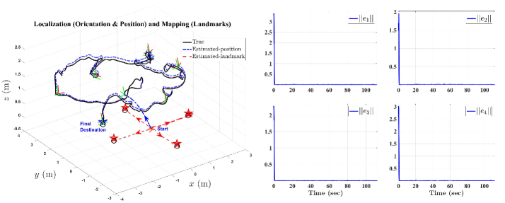
Figure 4: Experimental validation using dataset Vicon Room 2 01. Output performance of the proposed nonlinear observer for SLAM vs the true trajectory (on the left), and error trajectories (on the right).

Also, suppose that the initial estimates of the four landmark positions are $\hat{{\rm p}}_{1}\left(0\right)=\hat{{\rm p}}_{2}\left(0\right)=\hat{{\rm p}}_{3}\left(0\right)=\hat{{\rm p}}_{4}\left(0\right)=[0,0,0]^{\top}$. Let us supplement the dataset measurement noise with additional uncertainties. Thus, assume the group velocity vector $U_{m}$ to be corrupted with constant bias $b_{U}=\left[b_{\Omega}^{\top},b_{V}^{\top}\right]^{\top}$ such that $b_{\Omega}=[-0.0023,0.0249,0.0816]^{\top}({\rm rad/sec})$ and $b_{V}=[-0.0209,0.1216,0.0788]^{\top}({\rm m/sec})$. Moreover, let $U_{m}$ be contaminated with noise $n_{U}=\left[n_{\Omega}^{\top},n_{V}^{\top}\right]^{\top}$ such that $n_{\Omega}=\mathcal{N}\left(0,0.1\right)({\rm rad/sec})$ and $n_{V}=\mathcal{N}\left(0,0.1\right)({\rm m/sec})$ where $n_{\Omega}=\mathcal{N}\left(0,0.1\right)$ abbreviates randomly distributed noise with a zero mean and a standard deviation of $0.1$. The design parameters are selected as $\xi_{\star}^{\infty}=0.03$, $\ell_{\star}=1$, $\xi_{\star}^{0}=\bar{\delta}_{\star}=\underline{\delta}_{\star}=e_{\star}\left(0\right)+4$, $\alpha_{i}=0.05$, $\Gamma_{1}=3\mathbf{I}_{3}$, $\Gamma_{2}=10\mathbf{I}_{3}$, $k_{w}=5$, $k_{1}=10$, and $k_{2}=10$ for all $i=1,2,3,4$. Additionally, set the initial bias estimate to $\hat{b}_{U}\left(0\right)=\underline{\mathbf{0}}_{6}$.

Fig. 3 depicts the true angular and translational velocities plotted against their measured values heavily contaminated with noise and bias. Black center-line represents the true values, while magenta, blue, and red stand for the measured values. The output trajectories estimated by the proposed nonlinear observer for SLAM are presented in Fig. 4 where they are compared to the true trajectories of travel. In the left portion of Fig. 4, the robot trajectory of travel is indicated using a black center-line, while the final destinations of both the robot and the fixed landmarks are marked with black circles. The true vehicle orientation is shown with a green solid-line. The estimated trajectory of the robot’s motion is depicted as a blue center-line that starts at the origin and arrives to the final destination marked with a blue star ${\color[rgb]{0,0,1}\star}$. The estimated landmark trajectories are depicted as red dash-lines and the final landmark positions estimated by the observer appear as red stars ${\color[rgb]{1,0,0}\star}$. The vehicle orientation estimation is presented as a red solid-line. In the right portion of Fig. 4, the error convergence of $||e_{1}||$, $||e_{2}||$, $||e_{3}||$, and $||e_{4}||$ is plotted as a blue solid-line.

It becomes evident that, as illustrated by the left portion of Fig. 4, both robot’s and landmark position estimates, initiated at the origin, successfully arrive to their true final destinations. The right portion of Fig. 4 illustrates asymptotic convergence of the error trajectories of $e_{i}$ for the nonlinear observer for SLAM. As attested by Fig. 4, the proposed observer is able to successfully localize the unknown robot’s position while simultaneously mapping the unknown environment.

VI Conclusion

In this paper, a nonlinear observer on the Lie group of $\mathbb{SLAM}_{n}\left(3\right)$ for Simultaneous Localization and Mapping (SLAM) has been proposed. The observer is able to efficiently control the error by implementing predefined measures of transient and steady-state performance. For successful operation the observer requires measurements of angular and translational velocity, landmark measurements, and an inertial measurement unit (IMU). Systematic convergence is enabled by the transformation of the constrained error to its unconstrained form. The proposed observer design successfully handles unknown bias inevitably present in the velocity measurements. Experimental results reveal the robustness and effectiveness of the proposed nonlinear observer for concurrent estimation of the unknown pose and mapping of the unknown landmarks.

AUTHOR INFORMATION

Hashim A. Hashim (Member, IEEE) is an Assistant Professor with the Department of Engineering and Applied Science, Thompson Rivers University, Kamloops, British Columbia, Canada. He received the B.Sc. degree in Mechatronics, Department of Mechanical Engineering from Helwan University, Cairo, Egypt, the M.Sc. in Systems and Control Engineering, Department of Systems Engineering from King Fahd University of Petroleum & Minerals, Dhahran, Saudi Arabia, and the Ph.D. in Robotics and Control, Department of Electrical and Computer Engineering at Western University, Ontario, Canada.
His current research interests include stochastic and deterministic attitude and pose filters, Guidance, navigation and control, simultaneous localization and mapping, control of multi-agent systems, and optimization techniques.

Contact Information: hhashim@tru.ca.

Abdelrahman E.E. Eltoukhy received his BSc Degree in Production Engineering from Helwan University, Egypt, and obtained his MSc in Engineering and Management from the Politecnico Di Torino, Italy. He obtained his PhD degree from The Hong Kong Polytechnic University, Hong Kong. He is currently a Research Assistant Professor in Industrial and Systems Engineering department, The Hong Kong Polytechnic University, Hong Kong.
His current research interests include airline schedule planning, logistics and supply chain management, operations research, and simulation.

References

• [1] M. Montemerlo, S. Thrun, D. Koller, B. Wegbreit et al., “Fastslam: A factored solution to the simultaneous localization and mapping problem,” Aaai/iaai, vol. 593598, 2002.
• [2] J. Mullane, B.-N. Vo, M. D. Adams, and B.-T. Vo, “A random-finite-set approach to bayesian slam,” IEEE transactions on robotics, vol. 27, no. 2, pp. 268–282, 2011.
• [3] H. Durrant-Whyte and T. Bailey, “Simultaneous localization and mapping: part i,” IEEE robotics & automation magazine, vol. 13, no. 2, pp. 99–110, 2006.
• [4] Z. Gong, J. Li, Z. Luo, C. Wen, C. Wang, and J. Zelek, “Mapping and semantic modeling of underground parking lots using a backpack lidar system,” IEEE Transactions on Intelligent Transportation Systems, 2019.
• [5] D. E. Zlotnik and J. R. Forbes, “Gradient-based observer for simultaneous localization and mapping,” IEEE Transactions on Automatic Control, vol. 63, no. 12, pp. 4338–4344, 2018.
• [6] H. A. Hashim, “Guaranteed performance nonlinear observer for simultaneous localization and mapping,” IEEE Control Systems Letters, vol. 5, no. 1, pp. 91–96, 2021.
• [7] K.-H. Lee, J.-N. Hwang, G. Okopal, and J. Pitton, “Ground-moving-platform-based human tracking using visual slam and constrained multiple kernels,” IEEE transactions on intelligent transportation systems, vol. 17, no. 12, pp. 3602–3612, 2016.
• [8] L. M. Paz, J. D. Tardós, and J. Neira, “Divide and conquer: Ekf slam in $o(n)$,” IEEE Transactions on Robotics, vol. 24, no. 5, pp. 1107–1120, 2008.
• [9] S. Holmes, G. Klein, and D. W. Murray, “A square root unscented kalman filter for visual monoslam,” in 2008 IEEE International Conference on Robotics and Automation.   IEEE, 2008, pp. 3710–3716.
• [10] Y. Dong, S. Wang, J. Yue, C. Chen, S. He, H. Wang, and B. He, “A novel texture-less object oriented visual slam system,” IEEE Transactions on Intelligent Transportation Systems, 2019.
• [11] M. Kaess, A. Ranganathan, and F. Dellaert, “isam: Incremental smoothing and mapping,” IEEE Transactions on Robotics, vol. 24, no. 6, pp. 1365–1378, 2008.
• [12] G. Bresson, T. Feraud, R. Aufrere, P. Checchin, and R. Chapuis, “Real-time monocular slam with low memory requirements,” IEEE Transactions on Intelligent Transportation Systems, vol. 16, no. 4, pp. 1827–1839, 2015.
• [13] T. Zhang, K. Wu, J. Song, S. Huang, and G. Dissanayake, “Convergence and consistency analysis for a 3-d invariant-ekf slam,” IEEE Robotics and Automation Letters, vol. 2, no. 2, pp. 733–740, 2017.
• [14] T. Qin, P. Li, and S. Shen, “Vins-mono: A robust and versatile monocular visual-inertial state estimator,” IEEE Transactions on Robotics, vol. 34, no. 4, pp. 1004–1020, 2018.
• [15] R. Sim, P. Elinas, M. Griffin, J. J. Little et al., “Vision-based slam using the rao-blackwellised particle filter,” in IJCAI Workshop on Reasoning with Uncertainty in Robotics, vol. 14, no. 1, 2005, pp. 9–16.
• [16] P. Lourenço, B. J. Guerreiro, P. Batista, P. Oliveira, and C. Silvestre, “Simultaneous localization and mapping for aerial vehicles: a 3-d sensor-based gas filter,” Autonomous Robots, vol. 40, no. 5, pp. 881–902, 2016.
• [17] H. F. Grip, T. I. Fossen, T. A. Johansen, and A. Saberi, “Attitude estimation using biased gyro and vector measurements with time-varying reference vectors,” IEEE Transactions on Automatic Control, vol. 57, no. 5, pp. 1332–1338, 2012.
• [18] H. A. Hashim, L. J. Brown, and K. McIsaac, “Nonlinear stochastic attitude filters on the special orthogonal group 3: Ito and stratonovich,” IEEE Transactions on Systems, Man, and Cybernetics: Systems, vol. 49, no. 9, pp. 1853–1865, 2019.
• [19] H. A. Hashim, “Systematic convergence of nonlinear stochastic estimators on the special orthogonal group SO(3),” International Journal of Robust and Nonlinear Control, vol. 30, no. 10, pp. 3848–3870, 2020.
• [20] H. A. Hashim, L. J. Brown, and K. McIsaac, “Nonlinear pose filters on the special euclidean group SE(3) with guaranteed transient and steady-state performance,” IEEE Transactions on Systems, Man, and Cybernetics: Systems, pp. 1–14, 2019.
• [21] D. E. Zlotnik and J. R. Forbes, “Higher order nonlinear complementary filtering on lie groups,” IEEE Transactions on Automatic Control, vol. 64, no. 5, pp. 1772–1783, 2018.
• [22] H. A. Hashim and F. L. Lewis, “Nonlinear stochastic estimators on the special euclidean group SE(3) using uncertain IMU and vision measurements,” IEEE Transactions on Systems, Man, and Cybernetics: Systems, vol. PP, no. PP, pp. PP–PP, 2020.
• [23] H. Strasdat, “Local accuracy and global consistency for efficient visual slam,” Ph.D. dissertation, Department of Computing, Imperial College London, 2012.
• [24] T. A. Johansen and E. Brekke, “Globally exponentially stable kalman filtering for slam with ahrs,” in 2016 19th International Conference on Information Fusion (FUSION).   IEEE, 2016, pp. 909–916.
• [25] C. P. Bechlioulis and G. A. Rovithakis, “Robust adaptive control of feedback linearizable mimo nonlinear systems with prescribed performance,” IEEE Transactions on Automatic Control, vol. 53, no. 9, pp. 2090–2099, 2008.
• [26] H. A. Hashim, S. El-Ferik, and F. L. Lewis, “Neuro-adaptive cooperative tracking control with prescribed performance of unknown higher-order nonlinear multi-agent systems,” International Journal of Control, vol. 92, no. 2, pp. 445–460, 2019.
• [27] C. Hu, Z. Wang, Y. Qin, Y. Huang, J. Wang, and R. Wang, “Lane keeping control of autonomous vehicles with prescribed performance considering the rollover prevention and input saturation,” IEEE Transactions on Intelligent Transportation Systems, 2019.
• [28] F. Bullo and A. D. Lewis, Geometric control of mechanical systems: modeling, analysis, and design for simple mechanical control systems.   Springer Science & Business Media, 2004, vol. 49.
• [29] C. Wei, J. Luo, H. Dai, and G. Duan, “Learning-based adaptive attitude control of spacecraft formation with guaranteed prescribed performance,” IEEE transactions on cybernetics, vol. 49, no. 11, pp. 4004–4016, 2018.
• [30] C. Wei, J. Luo, B. Gong, M. Wang, and J. Yuan, “On novel adaptive saturated deployment control of tethered satellite system with guaranteed output tracking prescribed performance,” Aerospace Science and Technology, vol. 75, pp. 58–73, 2018.
• [31] H. A. Hashim, “Attitude determination and estimation using vector observations: Review, challenges and comparative results,” arXiv preprint arXiv:2001.03787, 2020.
• [32] M. Burri, J. Nikolic, P. Gohl, T. Schneider, J. Rehder, S. Omari, M. W. Achtelik, and R. Siegwart, “The EuRoC micro aerial vehicle datasets,” The International Journal of Robotics Research, vol. 35, no. 10, pp. 1157–1163, 2016.