Finite Horizon Discrete Models for Multi-Agent Control Systems with Coupled Dynamics

Abstract

The goal of this paper is to obtain online abstractions for coupled multi-agent systems in a decentralized manner. A discrete model which captures the motion capabilities of each agent is derived over a bounded time-horizon, by discretizing a corresponding overapproximation of the agent’s reachable states. The individual abstractions’ composition provides a correct representation of the coupled continuous system over the horizon and renders the approach appropriate for control synthesis under high-level specifications which are assigned to the agents over this time window. Sufficient conditions are also provided for the space and time discretization to guarantee the derivation of deterministic abstractions with tunable transition capabilities.

,

1 Introduction

During the last decades there has been an emerging focus on the problem of high-level planning for multi-agent systems by leveraging methods from formal verification, with applications in several domains such as robotics [1] and air traffic management [2]. In order to exploit these tools for dynamic agents, it is required to build a discretized model of the continuous system, which allows for the algorithmic synthesis of high-level plans. Specifically, the use of an appropriate abstract representation enables the conversion of discrete paths into sequences of feedback controllers which enable the continuous-time model to implement the high-level specifications. The aforementioned control synthesis problem has led to a significant research effort for the derivation of discrete state analogues of continuous control systems, also called abstractions, which can capture reachability properties of the original model. Abstractions for piecewise affine systems on simplices and rectangles were introduced in [3] and have been further studied in [4]. Closer related to the control framework that we adopt here for the derivation of the discrete models is the paper [5], which builds on the notion of In-Block Controllability [6]. According to this property, all pairs of states inside a block should be mutually reachable in finite time through a bounded control. Abstractions for nonlinear systems are derived in [7] based on convex overapproximations of reachable sets, and in [8] for polynomial and other classes of systems. Other approaches build on approximate system relations [9], and have been exploited to derive abstractions for nonlinear stabilizable [10], incrementally forward complete [11], and networked control systems [12].

Reducing the complexity of the derived abstractions constitutes a significant research challenge. Towards this end, on the fly algorithms integrating the abstraction and control synthesis were considered in [13]. In [14], multi-scale discrete models are introduced, whereas in [15], local Lipschitz properties of probability densities are considered to efficiently abstract stochastic systems into finite Markov Chains. Given the exponential complexity of the symbolic models with respect to the system’s state dimension, recent attention has been drawn on the consideration of abstractions for interconnected systems, based on discrete models for their building components. Towards this goal, compositional abstractions for stabilizable interconnected linear systems were provided in [16]. The work [17] establishes approximate bisimulations for discrete time interconnected systems under small-gain assumptions. An algorithm suitable for system components with sparse interconnections is proposed in [18]. Small-gain type assumptions are also leveraged in [19], whereas in [20], compositional abstractions for safety specifications are obtained for systems with monotone dynamics. In [21], sufficient conditions are given to obtain bisimilar compositional abstractions for networks of incrementally input-to-state stable stochastic systems. Abstractions of feedback linearizable systems in cascade form were given in [22], and continuous abstractions in the form of lower dimensional control system models are derived in [23]. Recent results focused more on verification consider also nonlinear coordinate transformations to provide decoupling abstractions for polynomial ODE’s [24].

Motivated by applications such as the coordination of robotic networks, we consider multi-agent systems evolving according to continuous-time dynamics. Assigning coupling feedback laws among appropriately nearby agents can provide an autonomous and scalable way to achieve collective objectives, including rendezvous to a common location and geometric formations while keeping the network connected and avoiding collisions [25]. Additionally, it may be required to combine such objectives with high-level tasks, including safety, sequential reachability, and timed specifications [26]. Such tasks can be assigned to the team or specific agents during runtime, and may need to be fulfilled within specific time bounds. Therefore, we consider agent dynamics that apart from typical interconnection terms encountered in their popular coordination schemes include also bounded additive inputs, which provide some control capabilities to each agent. We exploit this control freedom to construct an individual transition system for each agent over a bounded time horizon that is used for correct-by-design control synthesis. Despite of the available controllability, we only assume forward completeness for the dynamics and make no hypotheses about the network interconnection structure. This makes the compositional abstraction approaches discussed above in general not applicable to the systems we consider. Specifically, in [16], [20], and [21], the dynamics need to be linear, monotone, and incrementally input-to-state stable, respectively, which is not required here, whereas in [17], the system components satisfy a small-gain condition that we do not impose. The works [19] and [23] consider abstractions from discrete-state to discrete-state systems, and continuous-state to continuous-state systems, respectively, while in this paper, we focus on the continuous-state to discrete-state problem. Further, in [22], the systems need to have a cascade interconnection, whereas here, the results are applicable for any interconnection structure.

The agents’ abstractions are built over a fixed time horizon by discretizing an overapproximation of their corresponding reachable sets into cells and selecting a common time duration for their transitions. For appropriate space and time discretizations each agent can perform transitions from an initial cell to other “nearby” ones by the selection of a feedback controller for each such transition. Selecting a common time step for the agents’ abstractions enables the synchronization of their transitions and renders their product a correct representation of the coupled system. Thus, it is possible to synthesize correct-by-design control strategies for specifications that can be satisfied over the horizon by working exclusively at the discrete level. In addition, based on the agents’ dynamics over the horizon, we specify acceptable discretizations which provide abstractions with quantifiable transition possibilities for each agent. The approach builds in part on our recent works [27] and [28], where the whole workspace is discretized, using global bounds for the agents’ dynamics. The main contributions of the paper are summarized as follows. 1) We derive deterministic agent models, which facilitates their algorithmic exploitation. This is accomplished by assigning decentralized feedback laws to the agents for the execution of their transitions, that attenuate an appropriate part of the coupling with their neighbors. Compared to our previous results [27], [28], which provide deterministic abstractions for analogous agent dynamics, we now only require that the system is forward complete. 2) We derive heterogeneous discretizations for the agents by using local bounds for their dynamics. This results in discretizations that are coarser, and hence, of reduced complexity for agents with higher actuation and weaker couplings over the horizon. The abstractions are decentralized, in the sense that correctness of the individual discrete models’ composition is not based on any global information on the interconnection structure. This further enables the identification of interconnection structures and specifications where control synthesis can be performed by avoiding the composition of all subsystems. Preliminary results from this paper appear in [29]. However, we include here all proofs which were omitted in [29], an updated analysis, and a worked out example with simulations.

2 Preliminaries and Notation

We use the notation $|x|$ for the Euclidean norm of a vector $x\in\mathbb{R}^{n}$. Given $R>0$ and $x\in\mathbb{R}^{n}$, we define by $B(x;R):=\{y\in\mathbb{R}^{n}:|x-y|\leq R\}$ the closed ball with center $x\in\mathbb{R}^{n}$ and radius $R$, and $B(R):=B(0;R)$. Given two sets $A,B\subset\mathbb{R}^{n}$, their Minkowski sum is defined as $A+B:=\{x+y:x\in A,y\in B\}$. We say that $\beta:\mathbb{R}_{\geq 0}\times\mathbb{R}_{\geq 0}\to\mathbb{R}_{\geq 0}$ is of class $\mathcal{K}_{+}\mathcal{K}_{+}$, if $\beta(t,\cdot)$ and $\beta(\cdot,s)$ are continuous and strictly increasing for all $t,s\geq 0$. Also, given $U\subset\mathbb{R}^{n}$, we denote by $\mathcal{M}_{U}$ the set of measurable functions from $\mathbb{R}_{\geq 0}$ to $U$ and define ${\rm sat}_{r}:\mathbb{R}^{n}\to\mathbb{R}^{n}$ as ${\rm sat}_{r}(x)=x$ if $|x|\leq r$ and ${\rm sat}_{r}(x)=r\frac{x}{|x|}$ if $|x|>r$, $r>0$.

Given a multi-agent system with $N$ agents and an agent $i\in\mathcal{N}:=\{1,\ldots,N\}$ we use the notation $\mathcal{N}_{i}\subset\mathcal{N}\setminus\{i\}$ for the set of its neighbors, $N_{i}$ for its cardinality and define $\bar{\mathcal{N}}_{i}:=\mathcal{N}_{i}\cup\{i\}$. We consider an ordering of the agent’s neighbors, denoted by $j_{1},\ldots,j_{N_{i}}$ and define the $N_{i}$-tuple $j(i)=(j_{1}(i),\ldots,j_{N_{i}}(i))$. Whenever it is clear from the context, the argument $i$ will be omitted from the latter notation. The agents’ network is represented by a directed graph $\mathcal{G}:=(\mathcal{N},\mathcal{E})$ with vertex set $\mathcal{N}$ the agents’ index set and edge set $\mathcal{E}$ the ordered pairs $(\ell,i)$ with $i\in\mathcal{N}$ and $\ell\in\mathcal{N}_{i}$. A sequence $i_{0}i_{1}\cdots i_{m}$ with $(i_{\kappa-1},i_{\kappa})\in\mathcal{E}$, $\kappa=1,\ldots,m$, and $i_{0}=i_{m}$ is called a cycle. Given the nonempty sets $\mathcal{I}_{1},\ldots,\mathcal{I}_{N}$, their Cartesian product $\bm{\mathcal{I}}:=\mathcal{I}_{1}\times\cdots\times\mathcal{I}_{N}$, and an agent $i\in\mathcal{N}$ with neighbors $j_{1},\ldots,j_{N_{i}}\in\mathcal{N}$, the mapping ${\rm pr}_{i}:\bm{\mathcal{I}}\to\bm{\mathcal{I}}_{i}:=\mathcal{I}_{i}\times\mathcal{I}_{j_{1}}\times\cdots\times\mathcal{I}_{j_{N_{i}}}$ assigns to each $N$-tuple $(l_{1},\ldots,l_{N})\in\bm{\mathcal{I}}$ the $N_{i}+1$-tuple $(l_{i},l_{j_{1}},\ldots,l_{j_{N_{i}}})\in\bm{\mathcal{I}}_{i}$, i.e., the entries of agent $i$ and its neighbors. A transition system is a tuple $TS:=(Q,Q_{0},Act,\longrightarrow)$, where: $Q$ is a set of states; $Q_{0}\subset Q$ is a set of initial states; $Act$ is a set of actions; $\longrightarrow$ is a transition relation with $\longrightarrow\subset Q\times Act\times Q$. The transition system is said to be finite, if $Q$ and $Act$ are finite sets. We also denote an element $(q,a,q^{\prime})\in\longrightarrow$ as $q\overset{a}{\longrightarrow}q^{\prime}$ and define ${\rm Post}(q;a):=\{q^{\prime}\in Q:(q,a,q^{\prime})\in\longrightarrow\}$, for every $q\in Q$ and $a\in Act$. $TS$ is called deterministic, if $|{\rm Post}(q;a)|\leq 1$ for each $q\in Q$ and $a\in Act$, where $|\cdot|$ is used to denote the cardinality of a set. We say that $TS$ is nonblocking on $\bar{Q}\subset Q$, if for each $q\in\bar{Q}$, there exist $a\in Act$ with ${\rm Post}(q;a)\neq\emptyset$. Finally, given a domain $D\subset\mathbb{R}^{n}$, a cell decomposition $\mathcal{S}=\{S_{l}\}_{l\in\mathcal{I}}$ of $D$ is a partition of $D$ into uniformly bounded sets with $S_{l}\cap S_{\hat{l}}=\emptyset$ for all $l\neq\hat{l}$, and $\cup_{l\in\mathcal{I}}S_{l}=D$. Given a set $A\subset D$, we say that $\mathcal{S}$ is compliant with $A$, if for any $S\in\mathcal{S}$ with $S\cap A\neq\emptyset$ it holds that $S\subset A$.

3 Problem Formulation

In this section we provide the class of interconnected systems studied in the paper and formulate the decentralized abstraction problem that will be considered. We focus on multi-agent systems with dynamics

$$\dot{x}_{i}(t)=f_{i}(x_{i}(t),\textbf{x}_{j}(t))+v_{i}(t),x_{i}(t)\in\mathbb{R}^{n},i\in\mathcal{N},$$ (1)

where $\textbf{x}_{j}(t)(=\textbf{x}_{j(i)}(t)):=(x_{j_{1}}(t),\ldots,x_{j_{N_{i}}}(t))\in\mathbb{R}^{N_{i}n}$. We consider decentralized control laws consisting of a feedback term $f_{i}(\cdot)$, which depends on the states of $i$ and its neighbors, and an additive input $v_{i}$ that provides certain control freedom to the agents and is leveraged for their abstractions. These dynamics can describe several multi-agent controllers, including consensus, connectivity maintenance, rendezvous, and formation [25], which are encountered for instance in decentralized multi-robot coordination applications. Such interconnection protocols can also guarantee desired properties robustly with respect to the $v_{i}$’s, as for instance in [30], where network connectivity is robustly preserved among neighboring agents for all additive inputs respecting a certain magnitude bound. Alternatively, (1) can represent internal dynamics of the system, as in temperature regulation of interconnected rooms [31]. We will assume that each $f_{i}(\cdot)$ is locally Lipschitz, and that $v_{i}\in\mathcal{U}_{i}:=\mathcal{M}_{B(v_{\max}(i))}$, or equivalently, that

$$|v_{i}(t)|\leq v_{\max}(i),\forall t\geq 0,$$ (2)

for all $i\in\mathcal{N}$, and define $\mathcal{U}:=\mathcal{M}_{B(v_{\max}(1))\times\cdots\times B(v_{\max}(N))}$. In addition, we assume that system (1) is forward complete:

Assumption 1.

(Forward Completeness) For every initial condition $\textbf{X}_{0}\in\mathbb{R}^{Nn}$ and input $\bm{v}\in\mathcal{U}$ the solution $\textbf{x}(t,\textbf{X}_{0};\bm{v})$ of (1) is defined for all $t\geq 0$. Equivalently (see [32, Lemma 2.3(ii)]), there exists a function $\beta\in\mathcal{K}_{+}\mathcal{K}_{+}$ such that for any $\textbf{X}_{0}\in\mathbb{R}^{Nn}$ and $\bm{v}\in\mathcal{U}$

$$|\textbf{x}(t,\textbf{X}_{0};\bm{v})|\leq\beta(t,|\textbf{X}_{0}|),\forall t\geq 0.$$ (3)

Given any finite time horizon $[0,T]$ and the agents’ positions at $t=0$, we will discretize an overapproximation $\mathcal{R}_{i}([0,T])$ of each agent’s reachable set over $[0,T]$ and select a common transition time step $\delta t$ with $T=\ell\delta t$, $\ell\in\mathbb{N}$, to obtain its individual abstraction in a decentralized manner. We use the term decentralized to indicate that the construction of each agent’s symbolic model is based only on local network information. It is also required that the composition of the individual transition systems can capture correctly the behavior of the coupled system (1) over $[0,T]$. Assuming that a set of specifications which need to be fulfilled over a bounded time duration are assigned to the agents, we can select a horizon $[0,T]$ which is sufficient to infer about their satisfiability and leverage the abstractions to synthesize corresponding discrete plans. Such specifications can be timed reachability goals such as “each agent $i$ should reach region $A(i)$ between $\tau_{1}(i)$ and $\tau_{1}^{\prime}(i)$ units, and region $B(i)$ between $\tau_{2}(i)$ and $\tau_{2}^{\prime}(i)$ units”, with $0\leq\tau_{1}(i)<\tau_{1}^{\prime}(i)\leq\tau_{2}(i)<\tau_{2}^{\prime}(i)$, whose satisfiability can be checked over the finite time horizon $[0,T]$ with $T\equiv\max\{\tau_{2}^{\prime}(i),i=1,\ldots,N\}$. Then, after selecting a satisfying plan and obtaining the agents’ positions at the end of its execution, i.e., at $t=T$, the same procedure can be repeated for another task assignment over a new horizon $[T,T_{1}]$, by updating the abstractions, and analogously for subsequent horizons $[T_{\kappa},T_{\kappa+1}]$, $\kappa\geq 1$. This motivates also the term online to characterize these abstractions.

For the space discretization we will consider cell decompositions $\{S_{l}^{i}\}_{l\in\mathcal{I}_{i}}$ of the sets $\mathcal{R}_{i}([0,T])$, $i\in\mathcal{N}$. We denote by $\textbf{l}_{i}=(l_{i},l_{j_{1}},\ldots,l_{j_{N_{i}}})\in\bm{\mathcal{I}}_{i}(=\mathcal{I}_{i}\times\mathcal{I}_{j_{1}}\times\cdots\times\mathcal{I}_{j_{N_{i}}})$ the index tuple of the cells where agent $i$ and its neighbors belong and call it the cell configuration of $i$. Given an analogous cell configuration $\textbf{l}=(l_{1},\ldots,l_{N})\in\bm{\mathcal{I}}(=\mathcal{I}_{1}\times\cdots\times\mathcal{I}_{N})$ of all agents, we use the operator ${\rm pr}_{i}:\bm{\mathcal{I}}\to\bm{\mathcal{I}}_{i}$ from Section 2 to obtain the cell configuration $\textbf{l}_{i}={\rm pr}_{i}(\textbf{l})$ of $i$. The state set of each agent’s individual transition system is formed by the cells of its decomposition and its transition possibilities are affected only by the cells of its neighbors. In particular, given the cells of $i$ and its neighbors, a transition to a successor cell is enabled for $i$, if there exists a control law which can drive the agent to that cell at $\delta t$, as in Fig. 1, right. The control law needs to trigger this transition for all initial conditions of the agent and its neighbors in their cells, and irrespectively of the neighbors’ further evolution during the transition interval. For each agent, we consider also a set $\mathcal{R}_{i}([0,T-\delta t])$ containing its reachable states over $[0,T-\delta t]$ and such that the trajectories of $i$ initiated from $\mathcal{R}_{i}([0,T-\delta t])$ remain in $\mathcal{R}_{i}([0,T])$ up to time $\delta t$. Thus, if a transition is initiated from a cell in $\mathcal{R}_{i}([0,T-\delta t])$, agent $i$ should reach some cell in $\mathcal{R}_{i}([0,T])$ at $\delta t$. We will require that each agent’s transition system is nonblocking and deterministic, namely, that there exists an outgoing transition from each cell in $\mathcal{R}_{i}([0,T-\delta t])$, and each such transition is uniquely determined by the selected controller according to the transition requirement described above. A discretization which enables this property will be called well posed (see Fig. 1). The discussed abstraction requirements are summarized in the following problem formulation.

Figure 1: Illustration of space-time discretizations which are well posed (right) and non-well posed (left), respectively

.

Problem Formulation Given the time horizon $[0,T]$ and the agents’ initial conditions $X_{10},\ldots,X_{N0}$, determine appropriate overapproximations $\mathcal{R}_{i}([0,t])$ of their reachable sets over $[0,t]$, $t\in[0,T-\tau]$, for some $\tau\in(0,T)$, select a cell decomposition $\{S_{l}^{i}\}_{l\in\mathcal{I}_{i}}$ of each $\mathcal{R}_{i}([0,T])$, and choose a common time step $\delta t<\tau$, in order to (i) derive a deterministic transition system for each agent, which is nonblocking for all cells in $\mathcal{R}_{i}([0,T-\delta t])$; equivalently, establish that the discretization is well posed, and (ii) guarantee that any transition sequence in the composition of the agents’ abstractions, which is initiated from cells containing their initial conditions $X_{10},\ldots,X_{N0}$, is matched by trajectories of system (1) over the horizon that are generated by corresponding sequences of feedback controllers assigned to the agents.

4 Abstraction Domain and Transition Design

In this section we start building towards the solution of the problem formulated above. In particular, we provide the overapproximations of the agent’s reachable sets that will be discretized, and the control laws which are leveraged for their transitions. The purpose of each such controller is to attenuate part of the agent’s coupling during a transition, so that the resulting trajectory is only dependent on the discrete location of its neighbors.

4.1 Overapproximation of the Agents’ Reachable Sets

For the subsequent analysis, we will assume fixed the initial states $X_{10},\ldots,X_{N0}$ of all agents at the beginning of the horizon $[0,T]$. Let

$$\mathcal{R}_{\bar{\mathcal{N}}_{i}}([0,T])\supset\{{\rm pr}_{i}(\textbf{x}(t,\textbf{X}_{0};\bm{v})):t\in[0,T],\bm{v}\in\mathcal{U}\},$$ (4)

be an overapproximation of the states reachable by agent $i$ and its neighbors in $\mathbb{R}^{(N_{i}+1)n}$ over the interval $[0,T]$ (recall that $\bar{\mathcal{N}}_{i}=\mathcal{N}_{i}\cup\{i\}$). Due to (3), each $\mathcal{R}_{\bar{\mathcal{N}}_{i}}([0,T])$ can be selected bounded, e.g., we can pick $\mathcal{R}_{\bar{\mathcal{N}}_{i}}([0,T])=\{(x_{i},\textbf{x}_{j})\in\mathbb{R}^{(N_{i}+1)n}:|(x_{i},\textbf{x}_{j})|\leq\beta(t,|\textbf{X}_{0}|)\}$, with $\beta(\cdot)$ as given in (3). Hence, by continuity of the coupling terms there exist constants $M(i)>0$ such that

$$|f_{i}(x_{i},\textbf{x}_{j})|\leq M(i),\forall(x_{i},\textbf{x}_{j})\in\mathcal{R}_{\bar{\mathcal{N}}_{i}}([0,T]).$$ (5)

Next, let $\tau\in(0,T)$ be an upper bound on the transition duration and consider bounded overapproximations $\mathcal{R}_{i}([0,T-\tau])\supset\{x_{i}(t,\textbf{X}_{0};\bm{v}):t\in[0,T-\tau],\bm{v}\in\mathcal{U}\}$ of each agent’s reachable states in $\mathbb{R}^{n}$ over $[0,T-\tau]$. Also, define

$$c_{i}(\sigma):= (M(i)+v_{\max}(i))\sigma,$$ (6)

$$\mathcal{R}_{i}([0,t]):= \mathcal{R}_{i}([0,T-\tau])+B(c_{i}(t-T+\tau)).$$ (7)

The sets $\mathcal{R}_{i}([0,t])$, $t\in[T-\tau,T]$, depicted in Fig. 2, are the overapproximations of the agents’ reachable sets that will be used for the abstractions. Their key properties are provided in the following lemma, shown in the Appendix.

Lemma 1.

(Overapproximation Properties) For all $t\in[T-\tau,T]$, the sets $\mathcal{R}_{i}([0,t])$ in (7) satisfy

$$\mathcal{R}_{i}([0,t])+ B(c_{i}(T-t))=\mathcal{R}_{i}([0,T]),$$ (8)

$$\mathcal{R}_{i}([0,t])\supset \{x_{i}(s,\textbf{X}_{0};\bm{v}):s\in[0,t],\bm{v}\in\mathcal{U}\}.$$ (9)

Figure 2: Illustration of the sets $\mathcal{R}_{i}([0,T-\tau])\subset\mathcal{R}_{i}([0,T-\delta t])$ $\subset\mathcal{R}_{i}([0,T])$, for $0<\delta t<\tau<T$. All contain the exact reachable set $\mathcal{R}_{i}^{\rm exact}([0,T-\tau])=\{x_{i}(t,\textbf{X}_{0};\bm{v}):t\in[0,T-\tau]$, $\bm{v}\in\mathcal{U}\}$ of $i$ over $[0,T-\tau]$ and its initial condition $X_{i0}$.

4.2 Discrete Transition Control Design

In order to derive the transitions of each agent $i\in\mathcal{N}$, we exploit the following auxiliary system

$$\dot{z}_{i}(t)=g_{i}(z_{i}(t),\textbf{d}_{j}(t))+v_{i}(t),$$ (10)

with continuous disturbances $d_{j_{1}},\ldots,d_{j_{N_{i}}}:\mathbb{R}_{\geq 0}\to\mathbb{R}^{n}$. This approach is inspired by [33], where piecewise affine systems with disturbances are leveraged for the construction of hybridizations for nonlinear systems. These hybridizations are exploited to design robust controllers on simplices, whose objective, i.e., invariance control or control to a facet, is accomplished for all disturbances capturing the mismatch between the nonlinear model and the local affine approximations. Here the role of the disturbances is to capture the possible evolution of the agent’s neighbors over the transition interval by restricting them over appropriate time-varying bounded sets. Each $g_{i}:\mathbb{R}^{(N_{i}+1)n}\to\mathbb{R}^{n}$ is given by

$$g_{i}(x_{i},\textbf{x}_{j})={\rm sat}_{M(i)}(f_{i}(x_{i},\textbf{x}_{j})),$$ (11)

with $f_{i}(\cdot)$ and $M(i)$ as in (1) and (5), respectively, and is locally Lipschitz. Thus, we get from (5) and (11) that

$$g_{i}(x_{i},\textbf{x}_{j}) =f_{i}(x_{i},\textbf{x}_{j}),\forall(x_{i},\textbf{x}_{j})\in\mathcal{R}_{\bar{\mathcal{N}}_{i}}([0,T]),$$ (12)

$$|g_{i}(x_{i},\textbf{x}_{j})| \leq M(i),\forall(x_{i},\textbf{x}_{j})\in\mathbb{R}^{(N_{i}+1)n}.$$ (13)

Recalling also that the sets $\mathcal{R}_{i}([0,T])$ have been selected bounded, there exist constants $L_{1}(i),L_{2}(i)>0$ with

$$|g_{i}(x_{i},\textbf{x}_{j}) -g_{i}(x_{i},\textbf{y}_{j})|\leq L_{1}(i)|\textbf{x}_{j}-\textbf{y}_{j}|,$$ (14)

$$|g_{i}(x_{i},\textbf{x}_{j}) -g_{i}(y_{i},\textbf{x}_{j})|\leq L_{2}(i)|x_{i}-y_{i}|,$$ (15)

$$\forall x_{\kappa},y_{\kappa} \in\mathcal{R}_{\kappa}([0,T]),\kappa\in\bar{\mathcal{N}}_{i}.$$

The above bounds and Lipschitz constants of the vector fields $g_{i}(\cdot)$ will be used determine the size of acceptable space-time discretizations for the agents’ abstractions over the horizon.

We next define the specific control laws that are exploited to derive the agents’ transitions based on the auxiliary dynamics (10). Consider for each agent $i$ a cell decomposition $\mathcal{S}_{i}=\{S_{l}^{i}\}_{l\in\mathcal{I}_{i}}$ of $\mathcal{R}_{i}([0,T])$ and a time step $\delta t$. We select the diameter $d_{\max}(i)$ of each $\mathcal{S}_{i}$ as the diameter of a ball whose translation can cover each cell in $\mathcal{S}_{i}$, and pick for every $S_{l_{i}}^{i}\in\mathcal{S}_{i}$ a reference point $x_{l_{i},G}$ with

$$|x_{l_{i},G}-x|\leq d_{\max}(i)/2,\forall x\in S_{l_{i}}^{i}.$$ (16)

For each agent $i$ and cell configuration $\textbf{l}_{i}$ of $i$, define the feedback law $k_{i,\textbf{l}_{i}}:[0,\infty)\times\mathbb{R}^{(N_{i}+1)n}\to\mathbb{R}^{n}$, parameterized by $x_{i0}\in S_{l_{i}}^{i}$ and $w_{i}\in W_{i}$, as

$$k_{i,\textbf{l}_{i}}(t,x_{i},\textbf{x}_{j};x_{i0},w_{i}):= {\rm sat}_{v_{\max}(i)}(\bar{k}_{i,\textbf{l}_{i}}(t,x_{i},\textbf{x}_{j};x_{i0},w_{i})),$$ (17)

$$\bar{k}_{i,\textbf{l}_{i}}(t,x_{i},\textbf{x}_{j};x_{i0},w_{i}):= k_{i,\textbf{l}_{i},1}(t,x_{i},\textbf{x}_{j})$$

$$+k_{i,\textbf{l}_{i},2}(w_{i})+k_{i,\textbf{l}_{i},3}(x_{i0})$$ (18)

where

$$W_{i}:= B(v_{\max}(i))\subset\mathbb{R}^{n},$$ (19)

$$k_{i,\textbf{l}_{i},1}(t,x_{i},\textbf{x}_{j}):= g_{i}(\chi_{i}(t),\textbf{x}_{l_{j},G})-g_{i}(x_{i},\textbf{x}_{j}),$$ (20)

$$k_{i,\textbf{l}_{i},2}(w_{i}):= \lambda(i)w_{i},\lambda(i)\in[0,1),$$ (21)

$$k_{i,\textbf{l}_{i},3}(x_{i0}):= (x_{l_{i},G}-x_{i0})/\delta t,$$ (22)

with $g_{i}(\cdot)$ as given in (10). The function $\chi_{i}(\cdot)$ in (20) is a reference trajectory defined through the solution of the initial value problem

$$\dot{\chi}_{i}(t)=g_{i}(\chi_{i}(t),\textbf{x}_{l_{j},G}),\chi_{i}(0)=x_{l_{i},G},$$ (23)

where $x_{l_{i},G}$, respectively, the $N_{i}$-tuple $\textbf{x}_{l_{j},G}$, represent the reference points of $i$ and its neighbors. The feedback laws $k_{i,\textbf{l}_{i}}(\cdot)$ depend on the cell configuration $\textbf{l}_{i}$ of agent $i$, through the reference points $\textbf{x}_{l_{j},G}$ and $x_{l_{i},G}$ in (20) and (22), and the trajectory $\chi_{i}(\cdot)$ in (20) provided by (23). Note that if the control law $v_{i}(t)=k_{i,\textbf{l}_{i},1}(t,z_{i}(t),\textbf{d}_{j}(t))$ in (20) is applied to agent $i$’s auxiliary dynamics (10) with $z_{i}(\cdot)$ initiated from $x_{l_{i},G}$, then $z_{i}(\cdot)$ will coincide with the reference trajectory $\chi_{i}(\cdot)$. By adding also the component $k_{i,\textbf{l}_{i},2}(\cdot)$ in (21) to $v_{i}(t)$ in (10), with $i$ initiated again from $x_{l_{i},G}$, the agent will move according to the trajectory $t\mapsto\chi_{i}(t)+\lambda(i)w_{i}t=:\hat{z}_{i}(t)$ and reach the point $x:=\chi_{i}(\delta t)+\lambda(i)w_{i}\delta t$ inside the ball in Fig. 3 at $\delta t$. The point $x$ depends on the parameter $w_{i}$ from $W_{i}$ in (19), whose selection enables the agent to reach any alternative point inside that ball. The ball’s radius is

$$r_{i}:=\lambda(i)\delta tv_{\max}(i),$$ (24)

and is tuned through the parameter $\lambda(i)$ in (21), namely, the input part exploited to enable multiple transitions from each cell. By leveraging also the component $k_{i,\textbf{l}_{i},3}(\cdot)$, i.e., by applying the unsaturated version $\bar{k}_{i,\textbf{l}_{i}}(\cdot)$ of the feedback law, the agent can reach any point inside this ball from every initial condition in its cell, and perform a transition to any cell intersecting $B(\chi_{i}(\delta t);r_{i})$. This is shown in the following lemma.

Lemma 2.

(Trajectories of (10) Under Unsaturated Feedback) Consider a cell configuration $\textbf{l}_{i}$, the reference trajectory $\chi_{i}(\cdot)$ in (23), and $r_{i}$ as given by (24). Then, (i) for any $x_{i0}\in S_{l_{i}}^{i}$, $w_{i}\in W_{i}$, and continuous disturbances $\textbf{d}_{j}(\cdot)$, the solution $z_{i}(\cdot)\equiv z_{i}(\cdot;x_{i0},w_{i})$ of (10) with initial condition $z_{i}(0)=x_{i0}$ and $v_{i}(t)=\bar{k}_{i,\textbf{l}_{i}}(t,z_{i}(t),\textbf{d}_{j}(t);x_{i0},w_{i})$ with $\bar{k}_{i,\textbf{l}_{i}}(\cdot)$ as in (18), satisfies

$$z_{i}(t)=\frac{\delta t-t}{\delta t}(x_{i0}-x_{l_{i},G})+\lambda(i)w_{i}t+\chi_{i}(t),t\geq 0;$$ (25)

(ii) for any $x\in B(\chi_{i}(\delta t);r_{i})$, if we set

$$w_{i}:=(x-\chi_{i}(\delta t))/(\lambda(i)\delta t),$$ (26)

then $w_{i}\in W_{i}$ and $z_{i}(\delta t;x_{i0},w_{i})=x$ for all $x_{i0}\in S_{l_{i}}^{i}$.

To prove (i), we get from (18) and (20)–(23), that the solution of (10) with $z_{i}(0)=x_{i0}$ and $v_{i}(t)=\bar{k}_{i,\textbf{l}_{i}}(t,z_{i}(t),\textbf{d}_{j}(t);x_{i0},w_{i})$ is given as $z_{i}(t)=x_{i0}+\int_{0}^{t}(g_{i}(\chi_{i}(s),\textbf{x}_{l_{j},G})+\frac{1}{\delta t}(x_{l_{i},G}-x_{i0})+\lambda(i)w_{i})ds=x_{i0}+\frac{t}{\delta t}(x_{l_{i},G}-x_{i0})+\lambda(i)w_{i}t+\int_{0}^{t}g_{i}(\chi_{i}(s),\textbf{x}_{l_{j},G})ds=\frac{\delta t-t}{\delta t}(x_{i0}-x_{l_{i},G})+\lambda(i)w_{i}t+x_{l_{i},G}+\int_{0}^{t}g_{i}(\chi_{i}(s),\textbf{x}_{l_{j},G})ds=\frac{\delta t-t}{\delta t}(x_{i0}-x_{l_{i},G})+\lambda(i)w_{i}t+\chi_{i}(t)$. Hence, (25) holds. To show (ii), note that due to (24) and (26), $|w_{i}|\leq\frac{r_{i}}{\lambda(i)\delta t}\leq v_{\max}(i)$, and hence, by virtue of (19), $w_{i}\in W_{i}$. In addition, we get from (25) that $z_{i}(\delta t)=\chi_{i}(\delta t)+\lambda(i)w_{i}\delta t$, and thus, by (26), that $z_{i}(\delta t)=x$. The above result remains is fact also valid when the control law $k_{i,\textbf{l}_{i}}$ in (17) is applied, as long as the discretization guarantees that the saturation level of the controller is not exceeded. Such discretizations will be provided in Section 5. It will also be shown in the correctness results of Section 6 that such transitions can be performed from appropriate cell configurations by assigning these control laws to the coupled agents in (1).

Figure 3: Illustration of the reference trajectory and reachability capabilities of the control laws (20)–(22).

5 Well-Posed Decentralized Abstractions

Here, we build on the previous section to define the agents’ individual discrete models and provide space and time discretizations which lead to a deterministic and nonblocking transition system for each agent.

5.1 Individual Discrete Agent Models

To derive the transitions of each agent’s discrete model we leverage the system with disturbances (10) and control laws as the ones introduced in (17). The results are presented in a more general context, in order to focus on the desirable properties of the control laws irrespectively of their precise formulas and keep the flexibility of alternative control designs to the one in (17). We consider hybrid feedback laws parameterized by the agents’ initial conditions and a set of auxiliary parameters associated to the agent’s reachability capabilities. In particular, consider an agent $i\in\mathcal{N}$, cell decompositions $\mathcal{S}_{\kappa}=\{S_{l}^{\kappa}\}_{l\in\mathcal{I}_{\kappa}}$ of $\mathcal{R}_{\kappa}([0,T])$, $\kappa\in\bar{\mathcal{N}}_{i}(=\mathcal{N}_{i}\cup\{i\})$, a nonempty subset $W_{i}$ of $\mathbb{R}^{n}$, and a cell configuration $\textbf{l}_{i}$ of $i$. A control law $k_{i,\textbf{l}_{i}}(t,x_{i},\textbf{x}_{j};x_{i0},w_{i}):[0,\infty)\times\mathbb{R}^{(N_{i}+1)n}\to S\subset\mathbb{R}^{n}$, parameterized by $x_{i0}\in S_{l_{i}}^{i}$ and $w_{i}\in W_{i}$, which is locally Lipschitz continuous on $(x_{i},\textbf{x}_{j})$, will be called a $W_{i}$ feedback law, and a $v_{\max}(i)-W_{i}$ feedback law if its codomain satisfies $S=B(v_{\max}(i))$. In the sequel, whenever we refer to a space-time discretization $\{\mathcal{S}_{i}\}_{i\in\mathcal{N}}-\delta t$ (or $\{\mathcal{S}_{\kappa}\}_{\kappa\in\bar{\mathcal{N}}_{i}}-\delta t$ for some $i$), it will be implicitly assumed that each $\mathcal{S}_{i}=\{S_{l}^{i}\}_{l\in\mathcal{I}_{i}}$ is a cell decomposition of $\mathcal{R}_{i}([0,T])$, and, that $\delta t<\tau$ and $T=\ell\delta t$ for some $\ell\in\mathbb{N}$. The following definition formalizes each agent’s transition requirement, based on the auxiliary system (10) and knowledge of its neighbors’ discrete positions.

Definition 1.

(Transition Requirement) Consider an agent $i\in\mathcal{N}$, a space-time discretization $\{\mathcal{S}_{\kappa}\}_{\kappa\in\bar{\mathcal{N}}_{i}}-\delta t$, a cell configuration $\textbf{l}_{i}$ of $i$ with $S_{l_{\kappa}}^{\kappa}\subset\mathcal{R}_{\kappa}([0,T-\delta t])$ for all $\kappa\in\bar{\mathcal{N}}_{i}$, and a $W_{i}$ feedback law $v_{i}=k_{i,\textbf{l}_{i}}(t,x_{i},\textbf{x}_{j};x_{i0},w_{i})$. Given $w_{i}\in W_{i}$ and a cell index $l_{i}^{\prime}\in\mathcal{I}_{i}$, we say that $k_{i,\textbf{l}_{i}}$, $w_{i}$, $l_{i}^{\prime}$ satisfy the Transition Requirement (TR) if for each $x_{i0}\in S_{l_{i}}^{i}$ and disturbances $d_{\kappa}\in C(\mathbb{R}_{\geq 0};\mathbb{R}^{n})$, $\kappa\in\mathcal{N}_{i}$, with

$$d_{\kappa}(t)\in S_{l_{\kappa}}^{\kappa}+B(c_{\kappa}(t))$$ (27)

for all $t\in[0,\delta t]$, the solution $z_{i}(\cdot)$ of (10) with $v_{i}(t)=k_{i,\textbf{l}_{i}}(t,z_{i}(t),\textbf{d}_{j}(t);x_{i0},w_{i})$ and $z_{i}(0)=x_{i0}$, satisfies $z_{i}(\delta t)\in S_{l_{i}^{\prime}}^{i}$, where $c_{\kappa}(\cdot)$ is given in (6).

Note that according to the Transition Requirement, agent $i$ can perform a deterministic transition to cell $S_{l_{i}^{\prime}}^{i}$ precisely at $\delta t$ under the auxiliary dynamics (10) using the feedback law $k_{i,\textbf{l}_{i}}(\cdot)$ tuned by the corresponding parameter $w_{i}$. This is possible for all disturbances satisfying (27), which capture the evolution of $i$’s neighbors on $[0,\delta t]$. We next define well-posed discretizations for the agents, which guarantee that their abstractions are nonblocking and the Transition Requirement is satisfied by control laws respecting the bounds $v_{\max}(i)$.

Definition 2.

(Well-Posed Discretizations) Consider the space-time discretization $\{\mathcal{S}_{i}\}_{i\in\mathcal{N}}-\delta t$ (i) Given an agent $i\in\mathcal{N}$, we say that $\{\mathcal{S}_{\kappa}\}_{\kappa\in\bar{\mathcal{N}}_{i}}-\delta t$ is well posed for $i$, if for any initial cell configuration $\textbf{l}_{i}\in\bm{\mathcal{I}}_{i}$ with $S_{l_{\kappa}}^{\kappa}\subset\mathcal{R}_{\kappa}([0,T-\delta t])$ for all $\kappa\in\bar{\mathcal{N}}_{i}$, there exist a $v_{\max}(i)-W_{i}$ feedback law $k_{i,\textbf{l}_{i}}$, a vector $w_{i}\in W_{i}$, and a cell index $l_{i}^{\prime}\in\mathcal{I}_{i}$, which satisfy the Transition Requirement of Definition 1. (ii) We say that the space-time discretization $\{\mathcal{S}_{i}\}_{i\in\mathcal{N}}-\delta t$ is well posed, if $\{\mathcal{S}_{\kappa}\}_{\kappa\in\bar{\mathcal{N}}_{i}}-\delta t$ is well posed for each $i\in\mathcal{N}$.

Following the formalism in [28] to determine the actions of the transitions, consider a well-posed discretization $\{\mathcal{S}_{i}\}_{i\in\mathcal{N}}-\delta t$. Also, select for each $i$ and cell configuration $\textbf{l}_{i}\in\bm{\mathcal{I}}_{i}$ with $S_{l_{\kappa}}^{\kappa}\subset\mathcal{R}_{\kappa}([0,T-\delta t])$, $\kappa\in\bar{\mathcal{N}}_{i}$, a $v_{\max}(i)-W_{i}$ feedback law $k_{i,\textbf{l}_{i}}$, generating at least one transition, namely, so that $k_{i,\textbf{l}_{i}}$, $w_{i}$, $l_{i}^{\prime}$ satisfy the Transition Requirement for some $w_{i}\in W_{i}$, $l_{i}^{\prime}\in\mathcal{I}_{i}$, and define for all $l\in\mathcal{I}_{i}$

$$[w_{i}]_{(\textbf{l}_{i},l)}:=\{w_{i}\in W_{i}:k_{i,\textbf{l}_{i}},w_{i},l\;\textup{satisfy (TR)}\}.$$ (28)

The sets $[w_{i}]_{(\textbf{l}_{i},l)}$ represent the parameters in $W_{i}$ which enable a transition to cell $S_{l}^{i}$ under the control $k_{i,\textbf{l}_{i}}$ and are used to define the agents’ individual abstractions.

Definition 3.

(Individual Transition Systems) Consider a well-posed discretization $\{\mathcal{S}_{i}\}_{i\in\mathcal{N}}-\delta t$, an agent $i\in\mathcal{N}$, and for each cell configuration $\textbf{l}_{i}\in\bm{\mathcal{I}}_{i}$ with $S_{l_{\kappa}}^{\kappa}\subset\mathcal{R}_{\kappa}([0,T-\delta t])$, $\kappa\in\bar{\mathcal{N}}_{i}$, a $v_{\max}(i)-W_{i}$ feedback law $k_{i,\textbf{l}_{i}}$ which generates at least one transition. The individual transition system $TS_{i}:=(Q_{i},Q_{0i},Act_{i},$ $\longrightarrow_{i})$ of agent $i$ consists of: State set $Q_{i}:=\mathcal{I}_{i}$ (the cell indices of $\mathcal{S}_{i}$); Initial state set $Q_{0i}:=\{l_{i}\in\mathcal{I}_{i}:X_{i0}\in S_{l_{i}}^{i}\}$; Actions $Act_{i}:=\bm{\mathcal{I}}_{i}\times 2^{W_{i}}$; Transition relation $\longrightarrow_{i}\subset Q_{i}\times Act_{i}\times Q_{i}$ defined as follows. For any $l_{i},l_{i}^{\prime}\in Q_{i}$ and $\textbf{l}_{i}=(l_{i},l_{j_{1}},\ldots,l_{j_{N_{i}}})\in\bm{\mathcal{I}}_{i}$, $l_{i}\overset{(\textbf{l}_{i},[w_{i}])}{\longrightarrow_{i}}l_{i}^{\prime}$ iff $S_{l_{\kappa}}^{\kappa}\subset\mathcal{R}_{\kappa}([0,T-\delta t])$, $\kappa\in\bar{\mathcal{N}}_{i}$, $[w_{i}]=[w_{i}]_{(\textbf{l}_{i},l_{i}^{\prime})}$, and $[w_{i}]_{(\textbf{l}_{i},l_{i}^{\prime})}\neq\emptyset$. Also, define

$$\overline{{\rm Post}}_{i}(\textbf{l}_{i}) :=\cup_{[w_{i}]\in 2^{W_{i}}}{\rm Post}_{i}(l_{i};(\textbf{l}_{i},[w_{i}]))$$

$$= \{l_{i}^{\prime}\in\mathcal{I}_{i}:\,\exists\,[w_{i}]\in 2^{W_{i}}{\rm s.t.}\;l_{i}\overset{(\textbf{l}_{i},[w_{i}])}{\longrightarrow_{i}}l_{i}^{\prime}\},$$ (29)

providing all successor cells from configuration $\textbf{l}_{i}$.

Remark 1.

(i) Given a well-posed discretization, it follows from Definition 3 that the associated transition system $TS_{i}$ of each agent is nonblocking on $\bar{Q}_{i}=\{l\in\mathcal{I}_{i}:S_{l}^{i}\subset\mathcal{R}_{i}([0,T-\delta t])\}$. In particular, transitions from cell configurations with $S_{l_{\kappa}}^{\kappa}\subset\mathcal{R}_{\kappa}([0,T-\delta t])$, $\kappa\in\bar{\mathcal{N}}_{i}$ are considered, which suffices in order to capture the agents’ behavior up to the horizon end. (ii) From (28) and Definition 3, it follows that each $[w_{i}]$ in the action of a transition is uniquely determined by the successor cell. Thus, by recalling that a cell decomposition is also a partition, each $TS_{i}$ is deterministic.

5.2 Space and Time Discretizations

We next present sufficient conditions to obtain well-posed space-time discretizations for system (1). Since the abstraction is updated at the end of the horizon, it is convenient to consider different decomposition diameters for the agents. This enables us to derive coarser discretizations for agents with weaker couplings and less conservative control constraints, i.e., larger $v_{\max}(i)$, and hence, reduce the abstraction complexity. We therefore introduce for each agent the design constraint that the diameters of its neighbors’ decompositions satisfy

$$d_{\max}(j)\leq\mu(j,i)d_{\max}(i).$$ (30)

For these restrictions to be feasible, we require that

$$\mu(i_{0},i_{1})\mu(i_{1},i_{2})\cdots\mu(i_{m-1},i_{m})\geq 1,$$

$$\textup{for all cycles}\;i_{0}i_{1}\cdots i_{m}\;{\rm with}\;i_{0}=i_{m}\;{\rm in}\;\mathcal{G},$$ (31)

which is always satisfied if we select $\mu(j,i)=1$ for all $i\in\mathcal{N}$ and $j\in\mathcal{N}_{i}$. For the acceptable values of the discretizations, it is also convenient to define for each agent the following local network parameters

$$\bm{\mu}(i):= (\sum_{j\in\mathcal{N}_{i}}\mu(j,i)^{2})^{\frac{1}{2}},$$ (32)

$$\textbf{M}(i):= (\sum_{j\in\mathcal{N}_{i}}(M(j)+v_{\max}(j))^{2})^{\frac{1}{2}}.$$ (33)

To obtain the agents’ transitions according to Definition 3 we will use the control laws introduced in (17) and show that they do not exceed their saturation level during the transitions. We therefore derive bounds on the unsaturated components of (17) along the solutions of (10) in the following lemma, shown in the Appendix.

Lemma 3.

(Bounds on Control Components) Consider a discretization $\{\mathcal{S}_{i}\}_{i\in\mathcal{N}}-\delta t$ with decomposition diameters $d_{\max}(i)$, parameters $\lambda(i)\in[0,1)$, $\mu(j,i)\geq 0$, $j\in\mathcal{N}_{i}$, and assume that (30) and (31) hold. Given $i\in\mathcal{N}$, a cell configuration $\textbf{l}_{i}$ of $i$ with $S_{l_{\kappa}}^{\kappa}\subset\mathcal{R}_{\kappa}([0,T-\delta t])$ for all $\kappa\in\bar{\mathcal{N}}_{i}$, and continuous $d_{j_{1}},\ldots,d_{j_{N_{i}}}$ satisfying (27), denote by $z_{i}(\cdot)$ the solution of (10) with $v_{i}=k_{i,\textbf{l}_{i}}$ as in (17). Then, for each $x_{i0}\in S_{l_{i}}^{i}$ and $w_{i}\in W_{i}$, the components $k_{i,\textbf{l}_{i},1}(\cdot)$, $k_{i,\textbf{l}_{i},2}(\cdot)$, and $k_{i,\textbf{l}_{i},3}(\cdot)$ in (18) satisfy

$$|k_{i,\textbf{l}_{i},1}(t,x_{i}(t),\textbf{d}_{j}(t))| \leq L_{1}(i)\left(\bm{\mu}(i)\frac{d_{\max}(i)}{2}+\textbf{M}(i)t\right)$$

$$+L_{2}(i)|z_{i}(t) -\chi_{i}(t)|,\forall t\in[0,\delta t],$$ (34)

$$|k_{i,\textbf{l}_{i},2}(w_{i})| \leq\lambda(i)v_{\max}(i),$$ (35)

$$|k_{i,\textbf{l}_{i},3}(x_{i0})| \leq d_{\max}(i)/(2\delta t).$$ (36)

with $L_{1}(i)$, $L_{2}(i)$, and $v_{\max}(i)$ as given in (14), (15), and (2), respectively, $\bm{\mu}(i)$, $\textbf{M}(i)$ as defined in (32), (33), and the reference trajectory $\chi_{i}(\cdot)$ provided by (23).

Based on this lemma, we characterize discretizations where the controllers designed for the transitions do not exceed their saturation level over the transition interval.

Proposition 1.

(Discretizations Keeping Controller Below Saturation) Consider a discretization $\{\mathcal{S}_{i}\}_{i\in\mathcal{N}}-\delta t$ with decomposition diameters $d_{\max}(i)$, and parameters $\lambda(i)\in[0,1)$, $\mu(j,i)\geq 0$, $j\in\mathcal{N}_{i}$. Assume that (30), (31) hold, and that $d_{\max}(i)$, $\delta t$ satisfy:

$$\delta t\in\left(0,\frac{(1-\lambda(i))v_{\max}(i)}{L_{1}(i)\textbf{M}(i)+L_{2}(i)\lambda(i)v_{\max}(i)}\right),$$ (37)

$$d_{\max}(i)\in\left(0,\min\left\{\tfrac{2(1-\lambda(i))v_{\max}(i)\delta t}{1+(L_{1}(i)\bm{\mu}(i)+L_{2}(i))\delta t},\right.\right.$$

$$\hskip 30.00005pt\left.\left.\tfrac{2(1-\lambda(i))v_{\max}(i)\delta t-2(L_{1}(i)\textbf{M}(i)+L_{2}(i)\lambda(i)v_{\max}(i))\delta t^{2}}{1+L_{1}(i)\bm{\mu}(i)\delta t}\right\}\right),$$ (38)

with $L_{1}(i)$, $L_{2}(i)$, and $v_{\max}(i)$ as given in (14), (15), and (2), respectively, and $\bm{\mu}(i)$, $\textbf{M}(i)$ as defined in (32), (33). Also, let any $i\in\mathcal{N}$ and a cell configuration $\textbf{l}_{i}$ of $i$ with $S_{l_{\kappa}}^{\kappa}\subset\mathcal{R}_{\kappa}([0,T-\delta t])$ for all $\kappa\in\bar{\mathcal{N}}_{i}$. Then, for any $x_{i0}\in S_{l_{i}}^{i}$, $w_{i}\in W$ and continuous $d_{j_{1}},\ldots,d_{j_{N_{i}}}$ satisfying (27), the solution $z_{i}(\cdot)$ of (10) with $v_{i}(t)=k_{i,\textbf{l}_{i}}(t,z_{i}(t),\textbf{d}_{j}(t);x_{i0},w_{i})$ and $z_{i}(0)=x_{i0}$ satisfies $k_{i,\textbf{l}_{i}}(t,z_{i}(t),\textbf{d}_{j}(t);x_{i0},w_{i})=\bar{k}_{i,\textbf{l}_{i}}(t,z_{i}(t),\textbf{d}_{j}(t);x_{i0},w_{i})$ for all $t\in[0,\delta t]$, with $k_{i,\textbf{l}_{i}}$ and $\bar{k}_{i,\textbf{l}_{i}}$ as given by (17) and (18), respectively.

The proof of Proposition 1 is given in the Appendix. We next provide the desired sufficient conditions for well posed space-time discretizations together with the agents’ corresponding transition capabilities.

Theorem 2.

(Well-Posed Discretizations: Sufficient Conditions) Consider a discretization $\{\mathcal{S}_{i}\}_{i\in\mathcal{N}}-\delta t$ with decomposition diameters $d_{\max}(i)$, and assume that the hypotheses of Proposition 1 are fulfilled. Then, the space-time discretization is well posed for system (1). In particular, by selecting for each $i\in\mathcal{N}$ and cell configuration $\textbf{l}_{i}$ of $i$ with $S_{l_{\kappa}}^{\kappa}\subset\mathcal{R}_{\kappa}([0,T-\delta t])$, $\kappa\in\bar{\mathcal{N}}_{i}$, the control law $k_{i,\textbf{l}_{i}}$ in (17), it holds that $\overline{{\rm Post}}_{i}(\textbf{l}_{i})\neq\emptyset$, with $\overline{{\rm Post}}_{i}(\cdot)$ as defined in (29). Furthermore,

$$B(\chi_{i}(\delta t);r_{i})\subset\mathcal{R}_{i}([0,T]),$$ (39)

$$\overline{{\rm Post}}_{i}(\textbf{l}_{i})=\{l\in\mathcal{I}_{i}:S_{l}^{i}\cap B(\chi_{i}(\delta t);r_{i})\neq\emptyset\},$$ (40)

with $\chi_{i}(\cdot)$ and $r_{i}$ as given by (23) and (24), respectively.

For the proof, pick $i\in\mathcal{N}$, and a cell configuration $\textbf{l}_{i}$ of $i$ with $S_{l_{\kappa}}^{\kappa}\subset\mathcal{R}_{\kappa}([0,T-\delta t])$, $\kappa\in\bar{\mathcal{N}}_{i}$. Also, consider the reference trajectory $\chi_{i}(\cdot)$ in (23) which is defined for all $t\geq 0$. We first show that (39) is satisfied. Indeed, let any $x\in B(\chi_{i}(\delta t);r_{i})$. Then, we obtain from (24) that $|\chi_{i}(\delta t)-x|\leq\lambda(i)v_{\max}(i)\delta t$. Furthermore, we get from (13) and (23) that $|\chi_{i}(\delta t)-x_{l_{i},G}|\leq M(i)\delta t$. Thus, it follows from (6) that $x-x_{l_{i},G}\in B(c_{i}(\delta t))$. From the latter, (8), which implies that $\mathcal{R}_{i}([0,T-\delta t])+B(c_{i}(\delta t))=\mathcal{R}_{i}([0,T])$, and the fact that $x_{l_{i},G}\in\mathcal{R}_{i}([0,T-\delta t])$, we obtain that $x\in\mathcal{R}_{i}([0,T])$, which establishes (39).

Next, from (39) and the fact that $\cup_{l_{i}\in\mathcal{I}_{i}}S_{l_{i}}^{i}=\mathcal{R}_{i}([0,T])$, we get that $\{l\in\mathcal{I}_{i}:S_{l}^{i}\cap B(\chi_{i}(\delta t);r_{i})\neq\emptyset\}\neq\emptyset$. Thus, validity of (40) implies directly that $\overline{{\rm Post}}_{i}(\textbf{l}_{i})\neq\emptyset$. To show (40), note first that due to (28) and Definition 3, $\overline{{\rm Post}}_{i}(\textbf{l}_{i})=\{l\in\mathcal{I}_{i}:\exists\,w_{i}\in W_{i}\;\textup{s.t.}\;k_{i,\textbf{l}_{i}},w_{i},l\;{\rm satisfy}\;{\rm(TR)}\}$. Thus, proving (40) is equivalent to showing that for each $l\in\mathcal{I}_{i}$, $S_{l}^{i}\cap B(\chi_{i}(\delta t);r_{i})\neq\emptyset$ iff there exists $w_{i}\in W_{i}$ so that $k_{i,\textbf{l}_{i}}$, $w_{i}$, $l$ satisfy the Transition Requirement. For the given discretization, it follows from Proposition 1 and standard ODE arguments that the solution $z_{i}(\cdot)$ of (10) with $v_{i}(t)=k_{i,\textbf{l}_{i}}(t,z_{i}(t),\textbf{d}_{j}(t);x_{i0},w_{i})$ and $z_{i}(0)=x_{i0}$ coincides with the solution $\bar{z}_{i}(\cdot)$ of (10) with $v_{i}(t)=\bar{k}_{i,\textbf{l}_{i}}(t,\bar{z}_{i}(t),\textbf{d}_{j}(t);x_{i0},w_{i})$ and $\bar{z}_{i}(0)=x_{i0}$, for any continuous disturbances satisfying (27). Thus, to verify (40) we will equivalently show that

$$S_{l}^{i}\cap B(\chi_{i}(\delta t);r_{i})\neq\emptyset\iff$$

$$\exists\,w_{i}\in W_{i}\;\textup{s.t.}\;\bar{k}_{i,\textbf{l}_{i}}, w_{i},l\;{\rm satisfy}\;{\rm(TR)}$$ (41)

for any $l\in\mathcal{I}_{i}$. To prove (41), assume that $\bar{k}_{i,\textbf{l}_{i}}$, $w_{i}$, $l$ satisfy (TR), implying that for any continuous disturbances such that (27) holds, the solution $z_{i}(\cdot)$ of (10) with $v_{i}(t)=\bar{k}_{i,\textbf{l}_{i}}(t,z_{i}(t),\textbf{d}_{j}(t);x_{i0},w_{i})$ and $z_{i}(0)=x_{i0}\in S_{l_{i}}^{i}$ satisfies $z_{i}(\delta t)\in S_{l}^{i}$. From Lemma 2(i), we get that $z_{i}(\delta t)=\chi_{i}(\delta t)+\lambda(i)w_{i}\delta t$. Thus, we get from (19) and (24) that $z_{i}(\delta t)\in B(\chi_{i}(\delta t);r_{i})$, and since $z_{i}(\delta t)\in S_{l}^{i}$, that $S_{l}^{i}\cap B(\chi_{i}(\delta t);r_{i})\neq\emptyset$. Conversely, let $x\in S_{l}^{i}\cap B(\chi_{i}(\delta t);r_{i})\neq\emptyset$. Then, by selecting $w_{i}$ according to (26), it follows from Lemma 2(ii) that $w_{i}\in W_{i}$ and that the solution $z_{i}(\cdot)$ of (10) with $v_{i}(t)=\bar{k}_{i,\textbf{l}_{i}}(t,z_{i}(t),\textbf{d}_{j}(t);x_{i0},w_{i})$ and $z_{i}(0)=x_{i0}\in S_{l_{i}}^{i}$ satisfies $z_{i}(\delta t)=x\in S_{l}^{i}$ for all $x_{i0}\in S_{l_{i}}^{i}$. Thus, $\bar{k}_{i,\textbf{l}_{i}}$, $w_{i}$, $l$ satisfy (TR) and the proof is complete.

Remark 5.1.

From the acceptable values of $\delta t$ and $d_{\max}(i)$ in (37), (38), it is observed that the discretizations become finer for larger dynamics bounds/Lipschitz constants, and tighter input constraints. Further, if follows from (24) that for larger values of the parameters $\lambda(i)$ it is possible to increase the number of successor transitions from each cell and enhance the abstraction accuracy by considering finer discretizations.

6 Correctness and Exploitation

Having established the existence of well-posed discretizations, we will show that the composition of the corresponding discrete agent models provides a correct representation of (1) over the horizon $[0,T]$ and clarify how the abstractions can be used for control synthesis.

6.1 Correctness of the Abstraction

As the first step to prove correctness, we provide a lemma for well-posed discretizations, which guarantees that if a cell configuration of all agents intersects their exact reachable set at some $t^{*}\in[0,T-\delta t]$, any successor configuration will also intersect this set at $t^{*}+\delta t$. In addition, by assigning to each agent a feedback law which enables its transition, the solution of the closed loop coupled system (1) will drive all agents to their successor cells at $\delta t$ from the designated initial conditions of their transitions. The proof is given in the Appendix.

Lemma 6.1.

(One Step Correctness) Consider a well-posed discretization $\{\mathcal{S}_{i}\}_{i\in\mathcal{N}}-\delta t$ and a cell configuration $\textbf{l}=(l_{1},\ldots,l_{N})$ with $S_{l_{i}}^{i}\subset\mathcal{R}_{i}([0,T-\delta t])$ for all $i\in\mathcal{N}$. Also, assume that there exist a time $t^{*}\in[0,T-\delta t]$ and an input $\bm{v}\in\mathcal{U}$ such that each component of the solution of (1) satisfies $x_{i}(t^{*},\textbf{X}_{0};\bm{v})\in S_{l_{i}}^{i}$. Then, for any $l_{i}^{\prime}\in\overline{{\rm Post}}_{i}({\rm pr}_{i}(\textbf{l}))$, $i\in\mathcal{N}$, the following hold. (i) There exist $v_{\max}(i)-W_{i}$ feedback laws $k_{i,{\rm pr}_{i}(\textbf{l})}(\cdot)$ and parameters $w_{i}\in W_{i}$, such that the solution $\bm{\xi}(\cdot)$ of the closed loop system (1) with $v_{i}=k_{i,{\rm pr}_{i}(\textbf{l})}$ and initial condition $\bm{\xi}(0)=\textbf{x}(t^{*},\textbf{X}_{0};\bm{v})$ satisfies $\xi_{i}(\delta t)\in S_{l_{i}^{\prime}}^{i}$ for all $i$. (ii) There exists $\bm{u}\in\mathcal{U}$, with $\bm{u}(t)=\bm{v}(t)$ for all $t\in[0,t^{*})$, such that the solution of (1) satisfies $x_{i}(t^{*}+\delta t,\textbf{X}_{0};\bm{u})\in S_{l_{i}^{\prime}}^{i}$ for all $i$.

We next provide the definition of the product transition system based on the synchronization of the agents’ actions in their individual transition systems.

Definition 4.

(Product Transition System) (i) Consider a well posed discretization $\{\mathcal{S}_{i}\}_{i\in\mathcal{N}}-\delta t$, and each agent’s individual transition system $TS_{i}$ as given by Definition 3. The product transition system $TS_{\mathcal{P}}:=(Q,Q_{0},{\rm Act},\longrightarrow)$ consists of: State set $Q:=\bm{\mathcal{I}}=\mathcal{I}_{1}\times\cdots\times\mathcal{I}_{N}$; Initial state set $Q_{0}:=Q_{01}\times\cdots\times Q_{0N}$, $Q_{0i}:=\{l_{i}\in\mathcal{I}_{i}:X_{i0}\in S_{l_{i}}^{i}\}$, $i\in\mathcal{N}$; Actions ${\rm Act}:=\{[w_{1}]\times\cdots\times[w_{N}]:[w_{i}]\in 2^{W_{i}},i\in\mathcal{N}\}$; Transition relation $\longrightarrow\subset Q\times Act\times Q$ defined as follows. For any $\textbf{l}=(l_{1},\ldots,l_{N}),\textbf{l}^{\prime}=(l_{1}^{\prime},\ldots,l_{N}^{\prime})\in Q$, and $[w]=[w_{1}]\times\cdots\times[w_{N}]\in{\rm Act}$, $\textbf{l}\overset{[w]}{\longrightarrow}\textbf{l}^{\prime}$ iff $l_{i}\overset{({\rm pr}_{i}(\textbf{l}),[w_{i}])}{\longrightarrow_{i}}l_{i}^{\prime}$ for all $i\in\mathcal{N}$. (ii) A path of length $m\in\{0,\ldots\ell\}$ originating from $\textbf{l}^{0}$ in $TS_{\mathcal{P}}$, is a finite sequence of states $\textbf{l}^{0}\textbf{l}^{1}\cdots\textbf{l}^{m}$ such that $\textbf{l}^{0}\in Q_{0}$ and $\textbf{l}^{\kappa}\in\overline{{\rm Post}}(\textbf{l}^{\kappa-1}):=\cup_{[w]\in Act}{\rm Post}(\textbf{l}^{\kappa-1};[w])$ for all $\kappa\in\{1,\ldots,m\}$ if $m\neq 0$.

We next show that for well-posed discretizations, any path of length $m\in\{0,\ldots,\ell\}$ originating from certain $\textbf{l}^{0}\in Q_{0}$ in $TS_{\mathcal{P}}$ can be realized by a sampled trajectory of the continuous-time system (1) on $[0,m\delta t]$, initiated from $\textbf{X}_{0}$. In addition, when the cell decomposition of each set $\mathcal{R}_{i}([0,T])$ is compliant with $\mathcal{R}_{i}([0,T-\delta t])$, there always exists an outgoing transition from the final state of each path with length less than $\ell$, which also implies the existence of such paths.

Proposition 3.

(Correctness of Discrete Paths) Assume that the discretization is well posed and that $\textbf{l}^{0}\textbf{l}^{1}\cdots\textbf{l}^{m}$ is a path of length $m\in\{0,\ldots,\ell\}$ originating from $\textbf{l}^{0}$ in $TS_{\mathcal{P}}$. Then, there exists an input $\bm{v}\in\mathcal{U}$ such that each component $x_{i}(\cdot,\textbf{X}_{0};\bm{v})$ of the solution of (1) satisfies $x_{i}(\kappa\delta t,\textbf{X}_{0};\bm{v})\in S^{i}_{l_{i}^{\kappa}}$ for all $\kappa\in\{0,\ldots,m\}$.

The proof is performed by induction on segments of the path, i.e., by showing that for each $\kappa\in\{0,\ldots,m\}$ there exists $\bm{v}\in\mathcal{U}$ such that $x_{i}(\mathfrak{K}\delta t,\textbf{X}_{0};\bm{v})\in S^{i}_{l_{i}^{\mathfrak{K}}}$ for all $\mathfrak{K}\in\{0,\ldots,\kappa\}$ and $i\in\mathcal{N}$. For $\kappa=0$, this follows directly from the fact that each $X_{i0}\in S_{l_{i}^{0}}^{i}$, since $\textbf{l}^{0}\in Q_{0}$. Assume next that the induction hypothesis is valid for certain $\kappa\in\{0,\ldots,m-1\}$, implying that there exists $\bm{v}\in\mathcal{U}$ with $x_{i}(\kappa\delta t,\textbf{X}_{0};\bm{v})\in S^{i}_{l_{i}^{\kappa}}$, for all $i\in\mathcal{N}$. In addition, since $\textbf{l}^{\kappa+1}\in\overline{{\rm Post}}(\textbf{l}^{\kappa})$, we have from Definitions 3 and 4 that $S_{l_{i}^{\kappa}}^{i}\subset\mathcal{R}_{i}([0,T-\delta t])$ for all $i\in\mathcal{N}$. Thus, application of Lemma 6.1(ii) with $t^{*}=\kappa\delta t\leq T-\delta t$, $\textbf{l}=\textbf{l}^{\kappa}$, and $l_{i}^{\prime}=l_{i}^{\kappa+1}$, $i\in\mathcal{N}$ yields existence of an input $\bm{u}\in\mathcal{U}$ with $\bm{u}(t)=\bm{v}(t)$ for all $t\in[0,\kappa\delta t)$ and $x_{i}((\kappa+1)\delta t,\textbf{X}_{0};\bm{u})\in S_{l_{i}^{\kappa+1}}^{i}$ for all $i\in\mathcal{N}$. The latter together with the induction hypothesis for $\kappa$ establishes validity of the general induction step, i.e., that $x_{i}(\mathfrak{K}\delta t,\textbf{X}_{0};\bm{u})\in S_{l_{i}^{\mathfrak{K}}}^{i}$ for all $\mathfrak{K}\in\{0,\ldots,\kappa+1\}$ and $i\in\mathcal{N}$.

Corollary 6.2.

(Existence of Discrete Paths) Assume that the discretization is well posed and that each cell decomposition $\mathcal{S}_{i}=\{S_{l}^{i}\}_{l\in\mathcal{I}_{i}}$ of $\mathcal{R}_{i}([0,T])$ is compliant with $\mathcal{R}_{i}([0,T-\delta t])$. Then, the following hold. (i) For any path $\textbf{l}^{0}\textbf{l}^{1}\cdots\textbf{l}^{m}$ of length $m\in\{0,\ldots,\ell-1\}$ it holds that $\overline{{\rm Post}}(\textbf{l}^{m})\neq\emptyset$, implying that for any $\textbf{l}^{m+1}\in\overline{{\rm Post}}(\textbf{l}^{m})$, $\textbf{l}^{0}\textbf{l}^{1}\cdots\textbf{l}^{m}\textbf{l}^{m+1}$ is a path of length $m+1$. (ii) For any $m\in\{0,\ldots,\ell\}$, there exists a path $\textbf{l}^{0}\textbf{l}^{1}\cdots\textbf{l}^{m}$ of length $m$ in $TS_{\mathcal{P}}$.

For the proof, let $\textbf{l}^{0}\textbf{l}^{1}\cdots\textbf{l}^{m}$ be a path of length $m\in\{0,\ldots,\ell-1\}$. Then, we get from Proposition 3 that there exists $\bm{v}\in\mathcal{U}$ such that $x_{i}(m\delta t,\textbf{X}_{0};\bm{v})\in S^{i}_{l_{i}^{m}}$ for all $i\in\mathcal{N}$. Thus, since $m\delta t\leq T-\delta t$, we get from (9) applied with $t=T-\delta t$ that $S^{i}_{l_{i}^{m}}\cap\mathcal{R}_{i}([0,T-\delta t])\neq\emptyset$. Hence, by compliance (see end of Section 2), it follows that $S^{i}_{l_{i}^{m}}\subset\mathcal{R}_{i}([0,T-\delta t])$ for all $i\in\mathcal{N}$. Thus, since the discretization is well posed, we can select for each agent a cell $l_{i}^{m+1}\in\overline{{\rm Post}}_{i}({\rm pr}_{i}(\textbf{l}^{m}))$, which implies that $\textbf{l}^{m+1}\in\overline{{\rm Post}}(\textbf{l}^{m})$ and establishes validity of part (i). The proof of part (ii) follows directly from the inductive application of part (i) and the fact that $\textbf{l}^{0}$ is a path of length 0 in $TS_{\mathcal{P}}$.

Remark 6.3.

(i) From Lemma 6.1(i) and arguing analogously as in the above proofs, we also deduce the useful fact that for any path $\textbf{l}^{0}\textbf{l}^{1}\cdots\textbf{l}^{m}$ of length $m\in\{0,\ldots,\ell\}$ in $TS_{\mathcal{P}}$, there exist sequences of feedback controllers $k_{i,{\rm pr}_{i}(\textbf{l}^{0})}\ldots k_{i,{\rm pr}_{i}(\textbf{l}^{m-1})}$, $i\in\mathcal{N}$, which can be applied successively at the time intervals $[0,\delta t],\dots,[(m-1)\delta t,m\delta t]$ and guarantee that each agent $i$ will lie in cell $S_{l_{i}^{\kappa}}^{i}$ at $\kappa\delta t$, $\kappa=1,\ldots,m$. (ii) Consider an output map $H:\mathbb{R}^{Nn}\to O$, with the set $O$ referring to properties of interest associated to the agents’ joint state space, satisfying the compliance property that for any cell configuration $\textbf{l}=(l_{1},\ldots,l_{N})$ and $\textbf{x},\textbf{x}^{\prime}\in\mathbb{R}^{Nn}$ with $x_{i},x_{i}^{\prime}\in S_{l_{i}}^{i}$ for all $i\in\mathcal{N}$, it holds that $H(\textbf{x})=H(\textbf{x}^{\prime})$, and define $\bar{H}:\bm{\mathcal{I}}\to O$ by $\bar{H}(\textbf{l})=H(\textbf{x})$ for any x with $x_{i}\in S_{l_{i}}^{i}$. Then, for any output path $\bm{o}^{1}\bm{o}^{2}\cdots\bm{o}^{m}$ of length $m\leq\ell$, i.e., such that $\bm{o}^{\kappa}=\bar{H}(\bm{l}^{\kappa})$ for each $\kappa$ and some path $\textbf{l}^{0}\textbf{l}^{1}\cdots\textbf{l}^{m}$ in $TS_{\mathcal{P}}$, there exist sequences of feedback controllers as in (i) above, so that the solution $\bm{\xi}(\cdot,\textbf{X}_{0})$ of the closed loop system (1) satisfies $H(\bm{\xi}(\kappa\delta t,\textbf{X}_{0}))=\bm{o}^{\kappa}$ for each $\kappa$. (iii) The analysis and results of Sections 5 and 6 are also applicable when each agent’s initial states belong to a bounded set $\Omega_{i}$, with Assumption 1 guaranteeing again the existence of bounded overapproximations for the agents’ reachable sets from $\bm{\Omega}:=\Omega_{1}\times\cdots\times\Omega_{N}$ for the abstractions’ derivation.

6.2 Exploiting the Abstractions for Control Synthesis

Consider a set of specifications assigned to the agents, whose satisfiability can be checked over a bounded time horizon $[0,T]$. Then, the abstractions from Theorem 2 over this horizon can be exploited for control synthesis under these tasks through the following procedure.

Step 1. Given the agents’ initial positions and the time horizon, determine overapproximations of their reachable sets as in (7) and evaluate the corresponding bounds $M(i)$ and Lipschitz constants $L_{1}(i)$, $L_{2}(i)$ of the auxiliary dynamics.

Step 2. Based on the evaluated bounds and Lipschitz constants from Step 1, and the input bounds $v_{\max}(i)$, select design parameters $\lambda(i)$, $\mu(i,j)$ and leverage Theorem 2 to obtain a time step $\delta t$ and cell decompositions $\mathcal{S}_{i}$ of a well-posed discretization.

Step 3. Fix a reference point for every cell of the decompositions and derive the transition system $TS_{i}$ of each agent $i$ as follows. For each cell configuration $\textbf{l}_{i}$ compute the endpoint $\chi_{i}(\delta t)$ of the reference trajectory (23) and specify the cells which intersect $B(\chi_{i}(\delta t);r_{i})$ to obtain the transitions to the cells given by the right-hand side of (40). Note that the reference trajectories do not need to be stored and that no control laws are calculated at this step.

Step 4. Find satisfying discrete plans whose composition generates a path $\textbf{l}^{0}\textbf{l}^{1}\textbf{l}^{2}\cdots$ in the product transition system $TS_{\mathcal{P}}$ of Definition 4, that projects to a sequence of transitions $l_{i}^{0}\overset{(\textbf{l}_{i}^{0},[w_{i}]^{0})}{\longrightarrow_{i}}l_{i}^{1}\overset{(\textbf{l}_{i}^{1},[w_{i}]^{1})}{\longrightarrow_{i}}l_{i}^{2}\cdots$ for each agent.

Step 5. Select the continuous control laws to implement each agent’s discrete plan as follows. For each transition $l_{i}^{m}\overset{(\textbf{l}_{i}^{m},[w_{i}]^{m})}{\longrightarrow_{i}}l_{i}^{m+1}$, recalculate the trajectory $\chi_{i}(\cdot)$ corresponding to the cell configuration $\textbf{l}_{i}^{m}$, pick any $x\in B(\chi_{i}(\delta t);r_{i})\cap S_{l_{i}^{m+1}}^{i}$, compute $w_{i}$ from (26), and select the corresponding feedback $k_{i,\textbf{l}_{i}^{m}}(\cdot,\cdot,\cdot;\cdot,w_{i})$ from (17).

Recalculating the reference trajectories and evaluating the control laws in Step 5 can significantly alleviate the memory storage requirements of the abstraction scheme, since these operations are performed only for the transitions of the satisfying plan and not for all the transitions of the abstractions. Examples of specifications whose satisfiability can be checked in finite time include metric interval temporal logic (MITL) formulas of the form $\Diamond_{[1,1.5]}(R_{1}\land\Diamond_{[2.5,3.5]}R_{2})$, meaning “visit region $R_{1}$ within 1 and 1.5 time units, and once $R_{1}$ has been visited, visit region $R_{2}$ within 2.5 and 3.5 time units”, whose validity can be checked over the finite horizon $[0,5]$. Here, the timed eventually operator $\Diamond_{[a,b]}$ is used to denote that formula $\Diamond_{[a,b]}\phi$ is valid if $\phi$ becomes true at some time between $a$ and $b$ time units (see e.g., [26] for more details on the MITL semantics). Thus, desirable specifications include formulas with bounded temporal operators and any horizon of a length larger than the maximum over all sums of the upper bounds among nested temporal operators is sufficient to determine satisfiability of the formula (see [34]).

7 Example and Simulations

As an illustrative example we consider the coordination of five interconnected agents in $\mathbb{R}^{2}$. Agent 3 represents an autonomous ground vehicle operating on an inclined terrain formed by a hill centered at zero, whose height is given by $h(x):=C(1+\cos(\frac{\pi}{R}|x|))$, for $|x|<R$ and $h(x)=0$, for $|x|\geq R$. Its dynamics are $\dot{x}_{3}=f_{3}(x_{3})+v_{3}$, with $f_{3}(x_{3}):=-\nabla h(x_{3})$. The other agents are UAVs operating at the same height and thus, modeled with two dimensional dynamics. Agents 2 and 4 are coupled with agent 3 by $\dot{x}_{i}=x_{3}-x_{i}+v_{i}$, $i=2,4$, and agents 1 and 5 are coupled with 2 and 4 by $\dot{x}_{i}=x_{j}-x_{i}+v_{i}$, $(i,j)=(1,2),(5,4)$. The agents’ additive inputs satisfy $v_{\max}(3)\leq\frac{r}{2}$, $v_{\max}(i)\leq r$, $i=2,4$, and $v_{\max}(i)\leq 2r$, $i=1,5$, for certain $r\geq\frac{2C\pi}{R}$. The interconnection dynamics guarantee that agents 2, 3 and 3, 4, that are initially located at a distance no more than $2r$, maintain this distance bound during the system’s evolution. This allows them to exchange information for their feedback loop as well as high-level missions that are assigned during runtime, and can be verified by using the energy functions $V_{i3}(x_{i},x_{3})=\frac{1}{2}|x_{i}-x_{3}|^{2}$, $i=2,4$. Analogously, agents 1, 2 and 4, 5 maintain a distance of at most $5r$, where we consider enhanced sensing capabilities among aerial agents compared to the ones among UAVs and the ground vehicle. Hence, the overall network, whose topology is depicted in Fig. 4, remains connected during the system’s evolution for all input signals bounded by the given $v_{\max}(i)$. At some time instant (w.l.o.g. at $t=0$), the agents are assigned a set of timed specifications to reach the target boxes in Fig. 4. We assign the tasks $\Diamond_{[0.95,1]}(\hat{T}_{i}\land\Diamond_{[0.95,1]}T_{i})$ to agents $i=2,4$ (reach $\hat{T}_{i}$ between 0.95 and 1 time units, and once $\hat{T}_{i}$ is reached, reach $T_{i}$ between 0.95 and 1 time units), $\Diamond_{[1.95,2]}T_{i}$ to agents $i=1,5$, and $\Diamond_{[0.85,1.05]}\hat{T}_{3}\land\Diamond_{[1.95,2]}T_{3}$ to agent 3 (reach $\hat{T}_{3}$ between 0.85 and 1.05 time units, and $T_{3}$ between 1.95 and 2 time units). Based on the discussion at the end of Section 6.2, we select the horizon length $T=2$ that is sufficient to infer about satifiability of the tasks. From the bounds on the inter-agent distances, we obtain the following overapproximations of their reachable sets: $\mathcal{R}_{\bar{\mathcal{N}}_{3}}([0,T])=\mathcal{R}_{3}([0,T]):=X_{30}+B(rT)$; $\mathcal{R}_{\bar{\mathcal{N}}_{i}}([0,T]):=\{(x_{i},x_{3})\in\mathbb{R}^{4}:x_{3}\in\mathcal{R}_{3}([0,T])\;{\rm and}\;|x_{i}-x_{3}|<2r\}$, $\mathcal{R}_{i}([0,T]):=X_{i0}+B(3rT)$, $i=2,4$; $\mathcal{R}_{\bar{\mathcal{N}}_{i}}([0,T]):=\{(x_{i},x_{j})\in\mathbb{R}^{4}:x_{j}\in\mathcal{R}_{j}([0,T])\;{\rm and}\;|x_{i}-x_{j}|<5r\}$, $(i,j)=(1,2),(5,4)$, $R_{i}([0,T]):=X_{i0}+B(8rT)$, $i=1,5$. Using these sets and assuming that the parameters $C$ and $R$ in the dynamics of agent 3 satisfy $C\pi^{2}/R^{2}\leq 1$, we obtain the bounds $M(3)=\frac{r}{2}$, $M(i)=2r$, $i=2,4$, $M(i)=5r$, $i=1,5$ and Lipschitz constants $L_{1}(3)=0$, $L_{2}(3)=3$, and $L_{1}(i)=L_{2}(i)=1$, $i=1,2,4,5$. For the simulations we select the parameters $r=5$, $C=2$, and $R=2\pi$, related to the agents dynamics, the planning parameters $\lambda(i)=0.4$, $i=2,3,4$, $\lambda(i)=0.35$, $i=1,5$, and $\bm{\mu}(i)=1$ for all $i$, $\delta t=2/12$, i.e., $\ell=12$ time steps, and the largest corresponding values of $d_{\max}(i)$.

First, we use the individual transition system of agent 3 to determine all the cells reachable by the agent over the horizon, shown in blue in Fig. 4, and then select all the paths which satisfy its reachability specifications, depicted through the corresponding yellow cells. We next select one of these paths, illustrated through the red cells of the agent in the figure, and exploit the individual transition systems of agents 2 and 4, in order to determine their reachable cells for the selected path $l_{3}^{0}l_{3}^{1}\cdots l_{3}^{\ell}$ of agent 3. In particular, by denoting as $l_{2}^{0}$ the index of the cell where the initial state $X_{20}$ of agent 2 belongs, we evaluate the indices of its reachable cells at time $\kappa\delta t$ as $Q_{2}^{\kappa}={\rm Post}_{2}(Q_{2}^{\kappa-1},l_{3}^{\kappa-1})$, $\kappa=0,1,\ldots,\ell$. Note that $Q_{2}^{0}:=\{l_{2}^{0}\}$ and we have used the notation ${\rm Post}_{2}(Q_{2},l_{3}):=\cup_{l_{2}\in Q_{2}}{\rm Post}_{2}(l_{2};(l_{2},l_{3}))$ (recall that $(l_{2},l_{3})$ stands for the cell configuration of agent 2).

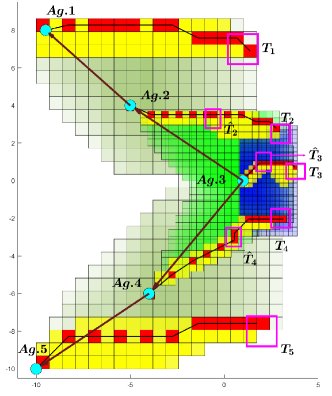
Figure 4: The agents’ initial positions are depicted with the cyan circles and the network topology is shown with the brown arrows. Each agent $i$ needs to reach the region(s) $T_{i}$ (and $\hat{T}_{i}$, $i=2,3,4$) depicted with the magenta box(es) within its specification deadlines. The selected discrete paths that satisfy all the agents’ specifications are depicted in red. The cells of agent 3 that satisfy its task are shown in yellow and the reachable cells of agents 2 and 4 for the selected path of 3 are in green. The cells of agents 2 and 4 that satisfy their tasks are shown in yellow and all corresponding reachable cells of agents 1 and 5 are in light green, with those satisfying further their specifications depicted in yellow.

Analogously, we evaluate the reachable cells of agent 4, depicted together with the ones of 2 with green in Fig. 4. Next, we determine the cells of 2 that reach its target $\hat{T}_{2}$ between 0.95 and 1 time units, and restrict its subsequent forward reachable cells to be originating from $\hat{T}_{2}$. After determining the ones from the latter that also reach the target $T_{2}$ within the next deadline, we perform a backward reachability algorithm and determine all the paths of agent 2 which satisfy both its reachability tasks, depicted with the corresponding yellow cells in Fig. 4 (analogously for agent 4). In a similar manner we derive the transitions of agents 1 and 5 corresponding to all the satisfying trajectories of 2 and 4, respectively, depicted with the light green cells in the figure, and compute all the discrete paths of 1 and 5 that satisfy their tasks, illustrated in yellow. Finally, we select a satisfying discrete trajectory for each of the agents 1, 2, 4, 5, depicted through the red cells in Fig. 4. The simulation results have been implemented in MATLAB with a running time of 15.395486 seconds, on a PC with an Intel(R) Core(TM) i5-4210U @ 1.7GHz processor. It is observed that the specifications can facilitate complexity reduction by restricting the satisfying paths of parent agents that are used as actions to compute the associated part of their children’s abstractions.

8 Conclusions and Future Work

We introduced an online abstraction framework which guarantees the existence of symbolic models for forward complete multi-agent systems under coupled constraints. For each agent, we derive an individual discrete model for an overapproximation of its reachable set over a finite time horizon. Further, the composition of the individual abstractions captures the evolution of the continuous-time system over the horizon. Ongoing work directions include the consideration of graph structures which can reduce the synthesis complexity and the consideration of agents with higher order dynamics. It is additionally desirable to address robustness of the transitions [35] and integrate the abstraction framework with receding horizon planing under high-level specifications [36].

Appendix A Appendix

Here we provide the proofs of Lemmas 1, 3, and 6.1, and Proposition 1. (of Lemma 1) The proof of (8) follows directly from (7), (6), and associativity of Minkowski addition. Indeed, we have that $\mathcal{R}_{i}([0,t])+B(c_{i}(T-t))=\mathcal{R}_{i}([0,T-\tau])+B(c_{i}(t-T+\tau))+B(c_{i}(T-t))=\mathcal{R}_{i}([0,T-\tau])+B(c_{i}(\tau))=\mathcal{R}_{i}([0,T])$. In order to show (9), let $s\in[0,t]$ and $\bm{v}\in\mathcal{U}$. Then, if $s\in[0,T-\tau]$, we have that $x_{i}(s,\textbf{X}_{0};\bm{v})\in\mathcal{R}_{i}([0,T-\tau])$ and thus, by (7), also that $x_{i}(s,\textbf{X}_{0};\bm{v})\in\mathcal{R}_{i}([0,t])$. Next, let $s\in[T-\tau,t]$. Since $t\leq T$, we obtain from (4) and (5) that $|\int_{T-\tau}^{s}(f_{i}(x_{i}(\sigma,\textbf{X}_{0};\bm{v}),\textbf{x}_{j}(\sigma,\textbf{X}_{0};\bm{v}))+v_{i}(\sigma))d\sigma|\leq(M(i)+v_{\max}(i))(s-T+\tau)$. Thus, since $s\leq t$, it follows from (6) that $\int_{T-\tau}^{s}(f_{i}(x_{i}(\sigma,\textbf{X}_{0};\bm{v}),\textbf{x}_{j}(\sigma,\textbf{X}_{0};\bm{v}))+v_{i}(\sigma))d\sigma\in B(c_{i}(t-T+\tau))$. From the latter, (7), and the fact that $x_{i}(T-\tau,\textbf{X}_{0};\bm{v})\in\mathcal{R}_{i}([0,T-\tau])$ and $x_{i}(s,\textbf{X}_{0};\bm{v})=x_{i}(T-\tau,\textbf{X}_{0};\bm{v})+\int_{T-\tau}^{s}(f_{i}(x_{i}(\sigma,\textbf{X}_{0};\bm{v}),$ $\textbf{x}_{j}(\sigma,\textbf{X}_{0};\bm{v}))+v_{i}(\sigma))d\sigma$, we get that (9) is fulfilled and the proof is complete. (of Lemma 3) By taking into account (13) and that the range of $k_{i,\textbf{l}_{i}}$ lies in $B(v_{\max}(i))$, the dynamics of (10) are bounded. Combined with their Lipschitz property, this implies that $z_{i}(\cdot)$ is well defined for all times and satisfies $|z_{i}(t)-x_{i0}|\leq\int_{0}^{t}|g_{i}(z_{i}(s),\textbf{d}_{j}(s))+k_{i,\textbf{l}_{i}}(s,z_{i}(s),\textbf{d}_{j}(s);x_{i0},w_{i})|ds\leq(M(i)+v_{\max}(i))t$. Consequently, we obtain from (6) that $z_{i}(t)-x_{i0}\in B(c_{i}(\delta t))$ for all $t\in[0,\delta t]$. Thus, since $x_{i0}\in S_{l_{i}}^{i}\subset\mathcal{R}_{i}([0,T-\delta t])$, and due to (8) it holds that $\mathcal{R}_{i}([0,T-\delta t])+B(c_{i}(\delta t))=\mathcal{R}_{i}([0,T])$, it follows that

$$z_{i}(t)\in\mathcal{R}_{i}([0,T]),\forall t\in[0,\delta t].$$ (42)

Analogously, since $S_{l_{\kappa}}^{\kappa}\subset\mathcal{R}_{\kappa}([0,T-\delta t])$ for all $\kappa\in\mathcal{N}_{i}$, we obtain from (27) that

$$d_{\kappa}(t)\in\mathcal{R}_{\kappa}([0,T]),\forall t\in[0,\delta t],\kappa\in\mathcal{N}_{i}.$$ (43)

In order to show (34), notice that due to (20) we have

$$k_{i,\textbf{l}_{i},1}(t,z_{i}(t),\textbf{d}_{j}(t))=[g_{i}(\chi_{i}(t),\textbf{x}_{l_{j},G})-g_{i}(z_{i}(t),\textbf{x}_{l_{j},G})]$$

$$\qquad+[g_{i}(z_{i}(t),\textbf{x}_{l_{j},G})-g_{i}(z_{i}(t),\textbf{d}_{j}(t))].$$ (44)

For the second difference on the right hand side of (44), we obtain from (14), (42), and (43) that $|g_{i}(z_{i}(t),\textbf{x}_{l_{j},G})-g_{i}(z_{i}(t),\textbf{d}_{j}(t))|\leq L_{1}(i)|(d_{j_{1}}(t)-x_{l_{j_{1}},G},\ldots,d_{j_{N_{i}}}(t)-x_{l_{j_{N}},G})|$. From the latter combined with (6), (16), and (27), we get that $|g_{i}(z_{i}(t),\textbf{x}_{l_{j},G})-g_{i}(z_{i}(t),\textbf{d}_{j}(t))|\leq L_{1}(i)(\sum_{\kappa\in\mathcal{N}_{i}}(\frac{d_{\max}(\kappa)}{2}+(M(\kappa)+v_{\max}(\kappa))t)^{2})^{\frac{1}{2}}$. Thus, it follows from (30), (32), (33), and the Cauchy Schwartz inequality that

$$|g_{i}(z_{i}(t),\textbf{x}_{l_{j},G})-g_{i}(z_{i}(t),\textbf{d}_{j}(t))|$$

$$\leq L_{1}(i)[\sum_{\kappa\in\mathcal{N}_{i}}(\mu(\kappa,i)d_{\max}(i)/2+(M(\kappa)+v_{\max}(\kappa))t)^{2}]^{\frac{1}{2}}$$

$$\leq L_{1}(i)[d_{\max}(i)^{2}/4\sum_{\kappa\in\mathcal{N}_{i}}\mu(\kappa,i)^{2}+d_{\max}(i)t(\sum_{\kappa\in\mathcal{N}_{i}}\mu(\kappa,i)^{2})^{\frac{1}{2}}$$

$$\times(\sum_{\kappa\in\mathcal{N}_{i}}(M(\kappa)+v_{\max}(\kappa))^{2})^{\frac{1}{2}}+t^{2}\sum_{\kappa\in\mathcal{N}_{i}}(M(\kappa)+v_{\max}(\kappa))^{2}]^{\frac{1}{2}}$$

$$=L_{1}(i)[(\sum_{\kappa\in\mathcal{N}_{i}}\allowbreak\mu(\kappa,i)^{2})^{\frac{1}{2}}d_{\max}(i)/2+(\sum_{\kappa\in\mathcal{N}_{i}}(M(\kappa)$$

$$+v_{\max}(\kappa))^{2})^{\frac{1}{2}}t]=L_{1}(i)(\bm{\mu}(i)d_{\max}(i)/2+\textbf{M}(i)t)$$

for all $t\in[0,\delta t]$. For the other difference in (44), it follows analogously to the derivation of (42) that $\chi_{i}(t)\in\mathcal{R}_{i}([0,T])$ for all $t\in[0,\delta t]$. From the latter combined with (42) and (15) we get that $|g_{i}(z_{i}(t),\textbf{x}_{l_{j},G})-g_{i}(\chi_{i}(t),\textbf{x}_{l_{j},G})|\leq L_{2}(i)|z_{i}(t)-\chi_{i}(t)|$ for all $t\in[0,\delta t]$. Hence, it follows from the evaluated bounds on the differences in (44) that (34) holds. Next, from (21) and (19) we get that (35) holds. Finally, by recalling that $x_{l_{i},G}$ satisfies (16), it follows from (22) that (36) is fulfilled. (of Proposition 1) To prove the proposition, let $\bar{t}:=\sup\{t\in[0,\delta t]:\forall s\in[0,t],|\bar{k}_{i,\textbf{l}_{i}}(s,z_{i}(s),$ $\textbf{d}_{j}(s);x_{i0},w_{i})|\leq v_{\max}(i)\}$ and note that due to (17), it suffices to show that $\bar{t}=\delta t$. By recalling that $S_{l_{\kappa}}^{\kappa}\subset\mathcal{R}_{\kappa}([0,T-\delta t])$ for all $\kappa\in\mathcal{N}_{i}$ and that $d_{j_{1}},\ldots,d_{j_{N_{i}}}$ satisfy (27), it follows from Lemma 3 that the components $k_{i,\textbf{l}_{i},1}(\cdot)$, $k_{i,\textbf{l}_{i},2}(\cdot)$, and $k_{i,\textbf{l}_{i},3}(\cdot)$ in (17) evaluated along the solution of (10) satisfy the bounds (34)–(36). Thus, due to (34), (23), and (16), we have that $|k_{i,\textbf{l}_{i},1}(0,z_{i}(0),\textbf{d}_{j}(0))|\leq\frac{(L_{1}(i)\bm{\mu}(i)+L_{2}(i))d_{\max}(i)}{2}$. The latter together with (36) and (35) imply by virtue of (38) that $|\bar{k}_{i,\textbf{l}_{i}}(0,z_{i}(0),\textbf{d}_{j}(0);\allowbreak x_{i0},w_{i})|<v_{\max}(i)$. Thus, $[0,\bar{t}]$ is well defined. We next show that

$$|\bar{k}_{i,\textbf{l}_{i}}(t,z_{i}(t),\textbf{d}_{j}(t);x_{i0},w_{i})|<v_{\max}(i),\forall t\in[0,\bar{t}],$$ (45)

which implies that $\bar{t}=\delta t$. Indeed, if $\bar{t}<\delta t$, we would have by (45) and continuity of $t\mapsto\bar{k}_{i,\textbf{l}_{i}}(t,z_{i}(t),\textbf{d}_{j}(t);\allowbreak x_{i0},w_{i})$ that $|\bar{k}_{i,\textbf{l}_{i}}(t,z_{i}(t),\textbf{d}_{j}(t);x_{i0},w_{i})|<v_{\max}(i)$ for all $t\in[0,\bar{t}+\varepsilon)$ and certain $\varepsilon\in(0,\delta t-\bar{t})$, contradicting the definition of $\bar{t}$. In order to show (45), note that due to the definition of $\bar{t}$, it holds for all $t\in[0,\bar{t}]$ that $k_{i,\textbf{l}_{i}}(t,z_{i}(t),\textbf{d}_{j}(t);x_{i0},w_{i})=\bar{k}_{i,\textbf{l}_{i}}(t,z_{i}(t),\textbf{d}_{j}(t);x_{i0},\allowbreak w_{i})$. From the latter and Lemma 2 we get that (25) holds. Combining this with (16), (19), and (34), we obtain that $|k_{i,\textbf{l}_{i},1}(t,z_{i}(t),$ $\textbf{d}_{j}(t))|\leq L_{1}(i)(\bm{\mu}(i)\frac{d_{\max}(i)}{2}+\textbf{M}(i)t)+L_{2}(i)(\frac{(\delta t-t)d_{\max}(i)}{2\delta t}\allowbreak+\lambda(i)v_{\max}(i)t)$, for all $t\in[0,\bar{t}]$. By taking into account the latter, (35), and (36), in order to show (45), we need to prove that $L_{1}(i)(\bm{\mu}(i)\frac{d_{\max}(i)}{2}+\textbf{M}(i)t)+\frac{d_{\max}(i)}{2\delta t}+L_{2}(i)(\frac{(\delta t-t)d_{\max}(i)}{2\delta t}+\lambda(i)v_{\max}(i)t)+\lambda(i)v_{\max}(i)<v_{\max}(i)$, for all $t\in[0,\bar{t}]$. Since the latter is linear with respect to $t$ and $[0,\bar{t}]\subset[0,\delta t]$, it suffices to verify it for $t=0$ and $t=\delta t$. Both cases follow directly from (38) and the proof is complete. (of Lemma 6.1) For the proof of both assertions let $l_{i}^{\prime}\in\overline{{\rm Post}}_{i}({\rm pr}_{i}(\textbf{l}))$ for each agent. Hence, given the cell configuration ${\rm pr}_{i}(\textbf{l})$ of each $i$, there exist a $v_{\max}(i)-W_{i}$ feedback law $v_{i}=k_{i,{\rm pr}_{i}(\textbf{l})}(t,x_{i},\textbf{x}_{j};x_{i0},w_{i})$, and a vector $w_{i}\in W_{i}$, such that $k_{i,{\rm pr}_{i}(\textbf{l})}$, $w_{i}$, $l_{i}^{\prime}$ satisfy the Transition Requirement (recall that the later refers to the system with disturbances (10)). Next, we select for each agent the initial condition $x_{i0}=x_{i}(t^{*},\textbf{X}_{0};\bm{v})$ and denote by $\bm{\xi}(\cdot)$ the solution of the closed loop system (1) with $v_{i}=k_{i,{\rm pr}_{i}(\textbf{l})}$, $i\in\mathcal{N}$ as selected above. By the Lipschitz properties on the $f_{i}$’s and $k_{i,{\rm pr}_{i}(\textbf{l})}$’s, this solution is unique and defined on the right maximal interval $[0,T_{\max})$. We will show that $T_{\max}=\infty$, and that for each agent $i\in\mathcal{N}$, the $i$-th component $\xi_{i}(\cdot)$ of $\bm{\xi}(\cdot)$ coincides with the solution of system (10) on $[0,\delta t]$ with $\textbf{d}_{j}(t)=\bm{\xi}_{j}(t)(=(\xi_{j_{1}}(t),\ldots,\xi_{j_{N_{i}}}(t))$ and the same initial condition $x_{i0}$. Indeed, consider the input $\bm{\omega}=(\omega_{1},\ldots,\omega_{N}):\mathbb{R}_{\geq 0}\to\mathbb{R}^{Nn}$ given as $\omega_{i}(t):=k_{i,{\rm pr}_{i}(\textbf{l})}(t,\xi_{i}(t),\bm{\xi}_{j}(t);x_{i0},w_{i})$, $t\in[0,T_{\max})$ and $\omega_{i}(t)=0$, $t\geq T_{\max}$, for all $i\in\mathcal{N}$. Then, since the image of each $k_{i,\textbf{l}_{i}}(\cdot)$ is contained in $B(v_{\max}(i))$, it follows that $|\omega_{i}(t)|\leq v_{\max}(i)$ for all $t\geq 0$, and hence, that $\bm{\omega}\in\mathcal{U}$. Thus, by denoting as $\bm{\eta}(\cdot,\textbf{x}_{0};\bm{\omega})$ the solution of (1) with input $\bm{\omega}(\cdot)$ and initial condition $\textbf{x}_{0}:=(x_{10},\ldots,x_{N0})$, we deduce from Assumption 1 that it is defined for all positive times. In addition, it follows from standard ODE arguments that

$$\bm{\xi}(t)=\bm{\eta}(t,\textbf{x}_{0};\bm{\omega}),\forall t\in[0,T_{\max}).$$ (46)

Thus, we get that $T_{\max}=\infty$, because otherwise it would hold that $\lim_{t\nearrow T_{\max}}\bm{\xi}(t)=\bm{\eta}(T_{\max},\textbf{x}_{0};\bm{\omega})$, contradicting maximality of $[0,T_{\max})$. Next, define $\bm{u}=(u_{1},\ldots,u_{N}):\mathbb{R}_{\geq 0}\to\mathbb{R}^{Nn}$ as

$$u_{i}(t):= v_{i}(t),t\in[0,t^{*}),$$

$$u_{i}(t):= \omega_{i}(t-t^{*}),t\geq t^{*}$$ (47)

for all $i\in\mathcal{N}$ and notice that $\bm{u}\in\mathcal{U}$. Using standard properties of time-invariant deterministic control systems, we obtain that $\bm{\eta}(t,x_{0};\bm{\omega})=\textbf{x}(t^{*}+t,\textbf{X}_{0};\bm{u})$, $\forall t\geq 0$. Hence, we get from (46) that

$$\bm{\xi}(t)=\textbf{x}(t^{*}+t,\textbf{X}_{0};\bm{u}),\forall t\geq 0$$ (48)

and since $t^{*}\leq T-\delta t$, we obtain from (48) and (4) that

$$(\xi_{i}(t),\bm{\xi}_{j}(t))\in\mathcal{R}_{\bar{\mathcal{N}}_{i}}([0,T]),\forall t\in[0,\delta t]$$ (49)

for all $i\in\mathcal{N}$. Thus, we get from (49) and (5) that $|f_{i}(\xi_{i}(t),\bm{\xi}_{j}(t))|\leq M(i)$ for all $t\in[0,\delta t]$. The latter together with (6) and the fact that $|k_{i,\textbf{l}_{i}}(\cdot)|$ is bounded by $v_{\max}(i)$, implies that

$$\xi_{i}(t)\in S_{l_{i}}^{i}+B(c_{i}(t)),\forall t\in[0,\delta t]$$ (50)

for all $i\in\mathcal{N}$. In addition, we have from (49) and (12) that $g_{i}(\xi_{i}(t),\bm{\xi}_{j}(t))=f_{i}(\xi_{i}(t),\bm{\xi}_{j}(t))$ for all $t\in[0,\delta t]$, $i\in\mathcal{N}$. Thus, for each $i\in\mathcal{N}$, $\xi_{i}(\cdot)$ coincides on $[0,\delta t]$ with the solution of system (10) with disturbances $\textbf{d}_{j}(t)=\bm{\xi}_{j}(t)$, input $v_{i}(t)=k_{i,\textbf{l}_{i}}(t,\xi_{i}(t),\textbf{d}_{j}(t);x_{i0},w_{i})$, and the selected $x_{i0}$, $w_{i}$ at the beginning of the proof. Due to (50), the disturbances satisfy (27). Hence, by recalling that $S_{l_{i}}^{i}\subset\mathcal{R}_{i}([0,T-\delta t])$ and that the selected $k_{i,{\rm pr}_{i}(\textbf{l})}$, $w_{i}$, $l_{i}^{\prime}$ satisfy the Transition Requirement, we deduce from Definition 1 that

$$\xi_{i}(\delta t)\in S_{l_{i}^{\prime}}^{i}$$ (51)

for all $i\in\mathcal{N}$, which establishes part (i) of the lemma. Part (ii) follows directly by selecting $\bm{u}(\cdot)$ as in (47), which by virtue of (51) and (48) implies that $x_{i}(t^{*}+\delta t,\textbf{X}_{0};\bm{u})\in S_{l_{i}^{\prime}}^{i}$ for all $i\in\mathcal{N}$. The proof is complete.

Appendix B Acknowledgements

This work was supported by the H2020 ERC Starting Grant BUCOPHSYS, the EU H2020 Co4Robots project, the Knut and Alice Wallenberg Foundation, the Swedish Foundation for Strategic Research (SSF), and the Swedish Research Council (VR).

References

- [1] S. G. Loizou and K. J. Kyriakopoulos. Automatic synthesis of multi-agent motion tasks based on LTL specifications. In Proceedings of the 43rd IEEE Conference on Decision and Control, pages 153–158, 2004.
- [2] S. M. Loos, D. Renshaw, and A. Platzer. Formal verification of distributed aircraft controllers. In Proceedings of the 16th international conference on Hybrid systems: computation and control, pages 125–130. ACM, 2013.
- [3] L. CGJM Habets and J. H. van Schuppen. Control of piecewise-linear hybrid systems on simplices and rectangles. In International Workshop on Hybrid Systems: Computation and Control, pages 261–274. Springer, 2001.
- [4] M. E. Brouke and M. Gannes. Reach control on simplices by piecewise affine feedback. SIAM Journal on Control and Optimization, 5(52):3261–3286, 2014.
- [5] M. K. Helwa and P. E. Caines. In-block controllability of affine systems on polytopes. In Proceedings of the 53rd IEEE Conference on Decision and Control, pages 3936–3942, 2014.
- [6] P. E. Caines and Y. J. Wei. The hierarchical lattices of a finite machine. Systems and Control Letters, (25):257–263, 1995.
- [7] G. Reissig. Computing abstractions of nonlinear systems. IEEE Transactions on Automatic Control, 56(11):2583–2598, 2011.
- [8] A. Abate, A. Tiwari, and S. Sastry. Box invariance in biologically-inspired dynamical systems. Automatica, 7(45):1601–1610, 2009.
- [9] P. Tabuada. Verification and Control of Hybrid Systems, A Symbolic Approach. Springer, New York, 2009.
- [10] P. Tabuada. An approximate simulation approach to symbolic control. IEEE Transactions on Automatic Control, 53(6):1406–1418, 2008.
- [11] M. Zamani, G. Pola, M. Mazo, and P. Tabuada. Symbolic models for nonlinear control systems without stability assumptions. IEEE Transactions on Automatic Control, 57(7):1804–1809, 2012.
- [12] M. Zamani, M. Mazo Jr, M. Khaled, and A. Abate. Symbolic abstractions of networked control systems. IEEE Transactions on Control of Network Systems, 2017.
- [13] G. Pola, A. Borri, and M. D. Di Benedetto. Integrated design of symbolic controllers for nonlinear systems. IEEE Transactions on Automatic Control, 57(2):534–539, 2012.
- [14] S. Mouelhi, A. Girard, and G. Gössler. Cosyma: a tool for controller synthesis using multi-scale abstractions. In Proceedings of the 16th international conference on Hybrid systems: computation and control, pages 83–88. ACM, 2013.
- [15] S. E. Z. Soudjani and A. Abate. Adaptive and sequential gridding procedures for the abstraction and verification of stochastic processes. SIAM Journal on Applied Dynamical Systems, 12(2):921–956, 2013.
- [16] Y. Tazaki and J.-ichi Imura. Bisimilar finite abstractions of interconnected systems. In International Workshop on Hybrid Systems: Computation and Control, pages 514–527. Springer, 2008.
- [17] G. Pola, P. Pepe, and M. D. di Benedetto. Symbolic models for networks of control systems. IEEE Transactions on Automatic Control, 61(11):3663–3668, 2016.
- [18] F. Gruber, E. S. Kim, and M. Arcak. Sparsity-sensitive finite abstraction. arXiv preprint arXiv:1704.03951.
- [19] E. Dallal and P. Tabuada. On compositional symbolic controller synthesis inspired by small-gain theorems. In Proceedings of the 54th IEEE Conference on Decision and Control, pages 6133–6138, 2015.
- [20] P.J. Meyer, A. Girard, and E. Witrant. Safety control with performance guarantees of cooperative systems using compositional abstractions. In Proceedings of the 5th IFAC Conference on Analysis and Design of Hybrid Systems, pages 317–322, 2015.
- [21] K. Mallik, S. E. Z. Soudjani, A.-K. Schmuck, and R. Majumdar. Compositional construction of finite state abstractions for stochastic control systems. arXiv preprint arXiv:1709.09546, 2017.
- [22] O. Hussien, A. Ames, and P. Tabuada. Abstracting partially feedback linearizable systems compositionally. IEEE Control Systems Letters, 1(2):227–232, 2017.
- [23] M. Rungger and M. Zamani. Compositional construction of approximate abstractions. In Proceedings of the 18th International Conference on Hybrid Systems: Computation and Control, pages 68–77, 2015.
- [24] A. Sogokon, K. Ghorbal, and T. T. Johnson. Decoupling abstractions of non-linear ordinary differential equations. In International Symposium on Formal Methods, pages 628–644. Springer, 2016.
- [25] M. Mesbahi and M. Egerstedt. Graph Theoretic Methods for Multiagent Networks. Princeton University Press, 2010.
- [26] A. Nikou, D. Boskos, J. Tumova, and D. V. Dimarogonas. On the timed temporal logic planning of coupled multi-agent systems. Automatica, 97:339–345, 2018.
- [27] D. Boskos and D. V. Dimarogonas. Abstractions of varying decentralization degree for coupled multi-agent systems. In Decision and Control (CDC), 2016 IEEE 55th Conference on, pages 81–86, 2016.
- [28] D. Boskos and D. V. Dimarogonas. Decentralized abstractions for multi-agent systems under coupled constraints. European Journal of Control, 45:1–16, 2019.
- [29] D. Boskos and D. V. Dimarogonas. Online abstractions for interconnected multi-agent control systems. In 20th IFAC World Congress, pages 15810–15815, 2017.
- [30] D. Boskos and D. V. Dimarogonas. Robustness and invariance of connectivity maintenance control for multiagent systems. SIAM Journal on Control and Optimization, 55(3):1887–1914, 2017.
- [31] M. Andreasson, D. V. Dimarogonas, H. Sandberg, and K. H. Johansson. Distributed control of networked dynamical systems: Static feedback, integral action and consensus. IEEE Transactions on Automatic Control, 59(7):1750–1764, 2014.
- [32] I. Karafyllis. Non-uniform in time robust global asymptotic output stability. Systems & control letters, 54(3):181–193, 2005.
- [33] A. Girard and S. Martin. Synthesis for constrained nonlinear systems using hybridization and robust controllers on simplices. IEEE Transactions on Automatic Control, 57(4):1046–1051, 2012.
- [34] V. Raman, A. Donzé, M. Maasoumy, R. M. Murray, A. Sangiovanni-Vincentelli, and S. A. Seshia. Model predictive control with signal temporal logic specifications. In Decision and Control (CDC), 2014 IEEE 53rd Annual Conference on, pages 81–87. IEEE, 2014.
- [35] G. Reissig, A. Weber, and M. Rungger. Feedback refinement relations for the synthesis of symbolic controllers. IEEE Transactions on Automatic Control, 62(4):1781–1796, 2017.
- [36] J. Tumova and D. V. Dimarogonas. Multi-agent planning under local LTL specifications and event-based synchronization. Automatica, 70:239–248, 2016.
- [37] E. Sontag. Mathematical Control Theory. Springer, New York, 2nd edition, 1998.