Primordial black holes and scalar-induced secondary gravitational waves from inflationary models with a noncanonical kinetic term

Abstract

With the enhancement mechanism provided by a noncanonical kinetic term with a peak, the amplitude of primordial curvature perturbations can be enhanced by seven orders of magnitude at small scales while keeping to be consistent with observations at large scales. The peak function and inflationary potential are not restricted in this mechanism. We use the Higgs model and T-model as examples to show how abundant primordial black hole dark matter with different mass and scalar induced secondary gravitational waves with different peak frequency are generated. We also show that the enhanced power spectrum for the primordial curvature perturbations and the energy density of the scalar induced secondary gravitational waves can have either a sharp peak or a broad peak. The primordial black holes with the mass around $10^{-14}-10^{-12}M_{\odot}$ produced with the enhancement mechanism can make up almost all dark matter, and the scalar induced secondary gravitational waves accompanied with the production of primordial black holes can be tested by the pulsar timing arrays and spaced based gravitational wave observatory. Therefore, the mechanism can be tested by primordial black hole dark matter and gravitational wave observations.

I Introduction

The detection of gravitational wave (GW) by the Laser Interferometer Gravitational Wave Observatory (LIGO) Scientific Collaboration and the Virgo Collaboration announced the dawn of the era of multimessenger astronomy [1, 2, 3, 4, 5, 6, 7, 8, 9, 10, 11, 12]. It was pointed out that these GWs may be emitted by the mergers of the stellar mass primordial black holes (PBHs) [13, 14]. PBHs are also proposed to account for dark matter (DM) due to the failure of direct detection of the particle DM [15, 16, 17, 18, 19, 20, 21, 22, 23, 24], and PBHs with the masses around $10^{-17}-10^{-15}M_{\odot}$ and $10^{-14}-10^{-12}M_{\odot}$ can make up almost all of DM because the abundances of PBHs at these mass windows are not constrained by observations. Furthermore, PBHs with the mass several times of the Earth’s can explain the Planet 9 which is a hypothetical astrophysical object in the outer solar system used to explain the anomalous orbits of trans-Neptunian objects [25]. PBHs are formed from the gravitational collapse of overdense regions with their density contrasts at the horizon reentry during radiation domination exceeding the threshold value [26, 27]. The overdense regions may be seeded from the primordial curvature perturbations generated during inflation. To produce enough abundance of PBH DM, the amplitude of the power spectrum of the primordial curvature perturbations should be $A_{s}\sim\mathcal{O}(0.01)$, while the constraint on the amplitude of the power spectrum at large scales from the cosmic microwave background (CMB) anisotropy measurements is $A_{s}=2.1\times 10^{-9}$ [28]. Therefore, the feasible way to produce enough abundance of PBH DM is by enhancing the amplitude of the power spectrum at least seven orders of magnitude to reach the threshold at small scales [29, 30, 31].

An effective way to enhance the power spectrum is through the ultra-slow-roll inflation [32, 33, 34]. For the single field inflation with a canonical scalar field, introducing an inflection point in the potential is a very economic way to realize the ultra-slow-roll inflation, hence producing abundant PBH DM [35, 36, 37, 38, 29, 39, 40]. However, it is not an easy task to achieve the big enhancement on the power spectrum while keeping the total number of e-folds around $50-60$ by fine tuning the model parameters [41, 42]. Nonminimal coupling to gravity and noncanonical kinetic terms were then considered [43, 44, 45, 46, 47, 48, 49, 50]. With the coupling parameter $1/M^{2}$ for the nonminimally derivative coupling to Einstein tensor generalizing to a special function $g(\phi)=h/\sqrt{1+(\phi-\phi_{p})^{2}/w^{2}}$, the inflationary model with the potential $\phi^{2/5}$ succeeds enhancing the power spectrum up to seven orders of magnitude at small scales [44, 45, 46], but both the potential and the coupling function $g(\phi)$ in this mechanism are restricted to the specific forms, and we need to fine tune the model parameters. Motivated by k inflation [51, 52] and G inflation [53, 54, 55, 56], the noncanonical kinetic term $[1+G_{p}(\phi)]\dot{\phi}^{2}/2$ with the peak function $G_{p}=h/(1+|\phi-\phi_{p}|/w)$ was proposed to enhance the power spectrum and produce abundant PBH DM [47]. Although the problem with the fine tuning of the model parameters is eased in this mechanism, but the potential was restricted to be $\phi^{2/5}$ [47] or $\phi^{1/3}$ [57]. This enhancement mechanism was then improved by generalizing the noncanonical kinetic term to be $G_{p}(\phi)+f(\phi)$ [58]. The function $G_{p}$ is used to enhance the power spectrum and the function $f(\phi)$ is acted as a chameleon field to modify the shape of the potential during inflation to make the model consistent with the observations. In this improved mechanism, it was shown that the inflation driven by the Higgs bonson with the potential $\lambda\phi^{4}/4$ in the standard model of particle physics satisfies the CMB constraints and provides the seed of PBH DM [58]. The improved mechanism also works for natural inflation [59] and T-model, and other peak functions are also possible, so the potential for the inflaton and the peak function are not restricted in this mechanism.

Accompanied by the formation of PBHs, the large scalar perturbations at small scales induce secondary GWs after the horizon reentry during the radiation dominated epoch [60, 61, 62, 63, 64, 65, 66, 67, 68, 69, 70, 71, 72, 73, 74, 75, 76, 77, 78, 79, 80, 81, 82, 83, 84, 85, 86, 87]. These scalar induced gravitational waves (SIGWs) that have a vast range of frequencies and consist of the stochastic background can be detected by pulsar timing arrays (PTA) [88, 89, 90, 91, 92] and the space based GW detectors such as Laser Interferometer Space Antenna (LISA) [93, 94], Taiji [95] and TianQin [96] in the future, and in turn disclose the properties of PBHs and primordial power spectrum at small scales.

In this paper, we elaborate on the mechanism proposed in Ref. [58] in detail. We consider a general peak function $G_{p}(\phi)=h/[1+\left(|\phi-\phi_{p}|/{w}\right)^{q}]$ and show that both sharp and broad peaks can be generated in this mechanism. The scale where the power spectrum is enhanced can be adjusted by the parameter $\phi_{p}$, and the peak shape of the power spectrum can be adjusted by the power index $q$. The paper is organized as follows. In Sec. II, we review the enhancement mechanism for primordial curvature perturbations proposed in Ref. [58]. We discuss the production of PBH DM and SIGWs from the Higgs model in Sec. III, and the generation of both PBH DM and SIGWs from T-model is considered in Sec. IV. We conclude the paper in Sec. V.

II The enhancement mechanism

In this section, we review the enhancement mechanism of the power spectrum at small scales proposed in Refs. [47, 58]. The action is

$$S=\int dx^{4}\sqrt{-g}\left[\frac{1}{2}R+X+G(\phi)X-V(\phi)\right],$$ (1)

where $X=-g_{\mu\nu}\nabla^{\mu}\phi\nabla^{\nu}\phi/2$, the noncanonical kinetic term may arise from scalar-tensor theory of gravity, G inflation [53] or k inflation [51, 52], and we take the convention $8\pi G=1$. After inflation, we expect $G(\phi)$ is negligible so that the noncanonical kinetic term disappears. The background equations are

$$3H^{2}=\frac{1}{2}\dot{\phi}^{2}+V(\phi)+\frac{1}{2}\dot{\phi}^{2}G(\phi),$$ (2)

$$\dot{H}=-\frac{1}{2}[1+G(\phi)]\dot{\phi}^{2},$$ (3)

$$\ddot{\phi}+3H\dot{\phi}+\frac{V_{\phi}+\dot{\phi}^{2}G_{\phi}/2}{1+G(\phi)}=0,$$ (4)

where $G_{\phi}=dG(\phi)/d\phi$ and $V_{\phi}=dV/d\phi$. The slow-roll parameters are defined as

$$\epsilon_{H}=-\frac{\dot{H}}{H^{2}},\quad\eta_{H}=-\frac{\ddot{\phi}}{H\dot{\phi}},\quad\epsilon_{G}=-\frac{G_{\phi}\dot{\phi}^{2}}{2V_{\phi}},$$ (5)

and the corresponding slow-roll conditions are

$$|\epsilon_{H}|\ll 1,\quad|\eta_{H}|\ll 1,\quad|\epsilon_{G}|\ll 1.$$ (6)

Under these slow-roll conditions, the background Eqs. (2) and (4) become

$$3H^{2}\approx V,$$ (7)

$$3H\dot{\phi}(1+G)+V_{\phi}\approx 0.$$ (8)

Combining the slow-roll background equations and the definitions of the slow-roll parameters, we have

$$\epsilon_{H}\approx\frac{\epsilon_{V}}{1+G},$$ (9)

$$\eta_{H}\approx\frac{\eta_{V}}{1+G}-\frac{\epsilon_{V}}{1+G}-\frac{\sqrt{2\epsilon_{V}}G_{\phi}}{(1+G)^{2}},$$ (10)

where the potential slow-roll parameters are defined as

$$\epsilon_{V}=\frac{1}{2}\left(\frac{V_{\phi}}{V}\right)^{2},\quad\eta_{V}=\frac{V_{\phi\phi}}{V}.$$ (11)

The power spectrum for the curvature perturbation is

$$\mathcal{P}_{\zeta}=\frac{H^{4}}{4\pi^{2}\dot{\phi}^{2}(1+G)}\approx\frac{V^{3}}{12\pi^{2}V_{\phi}^{2}}(1+G).$$ (12)

If the noncanonical kinetic term disappears, $G=0$, then we recover the result in standard slow-roll inflation. In other words, the noncanonical kinetic coupling $G$ can be used to enhance the scalar power spectrum at small scales. The scalar spectral index is

$$\begin{split}n_{s}-1&=\frac{d\ln\mathcal{P}_{\zeta}}{d\ln k}=-4\epsilon_{H}+2\eta_{H}-\frac{G_{\phi}}{1+G}\frac{\dot{\phi}}{H}\\ &\approx\frac{1}{1+G}\left(2\eta_{V}-6\epsilon_{V}-\frac{G_{\phi}}{1+G}\sqrt{2\epsilon_{V}}\right).\end{split}$$ (13)

Because tensor perturbations are independent of scalar perturbations and the additional noncanonical kinetic term doesn’t introduce any tensor degree of freedom, so the tensor power spectrum is the same as that in the canonical case

$$\mathcal{P}_{T}=\frac{2H^{2}}{\pi^{2}}\approx\frac{2V}{3\pi^{2}}.$$ (14)

Combining the scalar power spectrum (12) and the tensor power spectrum (14), we obtain the tensor-to-scalar ratio

$$r\simeq\frac{16\epsilon_{V}}{1+G}.$$ (15)

Since the Planck 2018 results give $A_{s}=2.1\times 10^{-9}$ at the pivotal scale $k_{*}=0.05$ Mpc^-1 [28], in order to produce enough abundance PBH DM, the scalar power spectrum should be enhanced at least seven orders of magnitude to reach $A_{s}\sim\mathcal{O}(0.01)$ at small scales. From the power spectrum (12), we see that a big peak in the coupling function $G(\phi)$ could realize this purpose. If we want the effect of the peak function is to enhance the power spectrum at small scales only while keeping the predictions of $n_{s}$ and $r$ at large scales, the peak function should be negligible away from the peak. Inspired by the coupling $\omega(\phi)=1/\phi$ in Brans-Dicke theory [97], a suitable peak function is [47]

$$G_{p}(\phi)=\frac{h}{1+|\phi-\phi_{p}|/w},$$ (16)

where $h$ gives the amplitude of the peak, $w$ controls the width of the peak, and $\phi_{p}$ determines the position of the peak in the power spectrum. Because the peak function is negligible at the CMB scale, from Eq. (13) and Eq. (15), the scalar spectral index and the tensor-to-scalar ratio reduce to the standard canonical slow-roll inflation results

$$n_{s}-1=2\eta_{V}-6\epsilon_{V},$$ (17)

$$r\simeq 16\epsilon_{V}.$$ (18)

With the help of Eqs. (7) and (8), we obtain the number of $e$-folds before the end of inflation at the horizon exit for the pivotal scale,

$$N=\int_{\phi_{e}}^{\phi_{*}}\frac{V}{V_{\phi}}d\phi+\Delta N,$$ (19)

where the first term is the $e$-folding number from the standard slow-roll inflation and the second term is from the peak function

$$\Delta N=\frac{V(\phi_{p})}{V_{\phi}(\phi_{p})}\int_{\phi_{p}+\Delta\phi}^{\phi_{p}-\Delta\phi}Gd\phi.$$ (20)

Although the peak function does not affect $n_{s}$ and $r$ at large scales, it influences $e$-folding number and contributes to about $20$ $e$-folds, henceforth effectively moves $\phi_{*}$ closer to $\phi_{e}$ in order to keep the total number of $e$-folds around $60$. In summary, the predictions of $n_{s}$ and $r$ at the pivotal scale for the inflationary model with the noncanonical kinetic term and $e$-folding number around 60 is the same as the canonical one with the $e$-folding number around $40$.

The Planck 2018 constraints [28, 98]

$$\begin{split}n_{s}=0.9649\pm 0.0042~{}(68\%\text{CL}),\\ r_{0.05}<0.06~{}(95\%\text{CL}),\end{split}$$ (21)

favor the parametrization

$$n_{s}=1-\frac{2}{N},$$ (22)

with $N=60$. This result can be obtained from many inflationary models [99, 100, 101]. With the $e$-folding number reducing to $40$, the formula (22) is inconsistent with the observational data, and it should be modified to

$$n_{s}=1-\frac{4}{3N},$$ (23)

to be consistent with the observational data with $N=40$. To get the inflationary potential with the prediction (23), we can use the method of potential reconstruction [102]. The reconstructed potential from the general parametrization

$$n_{s}=1-\frac{n+2}{2N},$$ (24)

is the chaotic inflation [103, 102]

$$V(\phi)=V_{0}\phi^{n},$$ (25)

and the corresponding tensor-to-scalar ratio is

$$r=\frac{4n}{N}.$$ (26)

Comparing Eq. (24) to Eq. (23), we get $n=2/3$, and the predictions are

$$n_{s}=0.967,\quad r=0.067,$$ (27)

where the tensor-to-scalar ratio is a bit large compared with the observational constraints (21). To obtain a smaller tensor-to-scalar ratio, from Eq. (26), we need a smaller $n$. For the sake of simplicity, we consider $n=1/3$, and the predictions are

$$n_{s}=0.971,\quad r=0.033.$$ (28)

In fact, the allowed values of $n$ from the observational constraints are broad, for example, the potential with $n=2/5$ discussed in Ref. [47] gives

$$n_{s}=0.970,\quad r=0.040,$$ (29)

which is consistent with the observational constraints. On the other hand, the $e$-folding number contributed from the peak function is not exact $20$, it depends on the model parameters. If the peak function contributes $25$ $e$-folds, the effective number of $e$-folds is $35$, from Eq. (24) and Eq. (26), the potential with $n=1/3$ and $N=35$ gives $n_{s}=0.967$ and $r=0.038$ which satisfy the observational constraints (21). Therefore, for suitable model parameters, the predictions of these models could be consistent with CMB constraints.

Because the effective $e$-folding number is about $40$, the usual inflationary potentials that satisfy the observational constraints with $N\sim 60$ would become incompatible with CMB observations with the enhancement mechanism. Therefore, the application of this mechanism is limited. To overcome this limitation, we take the advantage of the noncanonical kinetic term with a peak function and the success of the power-law potential $U(\Phi)=U_{0}\Phi^{n}$, so we take the form of the noncanonical coupling function to be

$$G(\phi)=G_{p}(\phi)+f(\phi),$$ (30)

where the peak function $G_{p}(\phi)$ is used to enhance the scalar power spectrum at small scales, the function $f(\phi)$ is acted as a chameleon field so that the potential $V(\phi)$ is adjusted to become the power-law potential $U(\Phi)$. More specifically, around the peak $f(\phi)\ll G_{p}(\phi)$, the peak function enhances the scalar power spectrum and contributes about 20 $e$-folds. Away from the peak we use the function $f(\phi)$ to change the noncanonical scalar field with the potential $V(\phi)$ to the canonical scalar field $\Phi$ with the potential $U(\Phi)$. In particular, under the transformation

$$d\Phi=\sqrt{1+f(\phi)}d\phi,\quad U(\Phi)=V[\phi(\Phi)],$$ (31)

the action (1) becomes

$$S=\int dx^{4}\sqrt{-g}\left[\frac{1}{2}R-\frac{1}{2}g_{\mu\nu}\nabla^{\mu}\Phi\nabla^{\nu}\Phi-U(\Phi)\right].$$ (32)

With the help of the chameleon function $f(\phi)$, we arrive at the standard case with the canonical scalar field $\Phi$, so at large scales the scalar spectral index and the tensor-to-scalar ratio are

$$n_{s}-1\simeq 2\eta_{U}-6\epsilon_{U},$$ (33)

$$r\simeq 16\epsilon_{U},$$ (34)

where $\epsilon_{U}$ and $\eta_{U}$ are

$$\epsilon_{U}=\frac{1}{2}\left(\frac{U_{\Phi}}{U}\right)^{2},\quad\eta_{U}=\frac{U_{\Phi\Phi}}{U}.$$ (35)

Therefore, the effect of the function $f(\phi)$ is to reshape the potential $V(\phi)$ to $U(\Phi)$ so that the predictions could be consistent with the observational constraints. In other words, for a given potential $V(\phi)$, from the transformation (31), we can find a corresponding function $f(\phi)$ and keep the predictions for $n_{s}$ and $r$ the same as that given by the effective potential $U(\Phi)$. For example, for the power-law potential $U(\Phi)=U_{0}\Phi^{n}$, the relation between $f(\phi)$ and potential $V(\phi)$ is

$$f(\phi)=\frac{1}{n^{2}}\left(\frac{1}{U_{0}}\right)^{2/n}V^{\frac{2}{n}-2}V_{\phi}^{2}.$$ (36)

The chaotic inflation with $n=1/3$ and $N\approx 40$ is consistent with the observational constraints as discussed above, so the potential $V(\phi)$ is not restricted to be a specific form.

Besides the loose restriction on the potential, to enhance the power spectrum, the peak function $G_{p}(\phi)$ is not restricted to the form (16) too. The peak function with a similar form as Eq. (16) can also successfully enhance the scalar power spectrum to produce abundant PBH DM and contribute about 20 $e$-folds, such as the peak function

$$G_{p}=\frac{h}{\sqrt{1+\left(\frac{\phi-\phi_{p}}{w}\right)^{2}}},$$ (37)

which is discussed in Refs. [44, 47]. In this paper, we consider a general peak function

$$G_{p}(\phi)=\frac{h}{1+\left(|\phi-\phi_{p}|/{w}\right)^{q}},$$ (38)

where the power index $q$ controls the shape of the enhanced power spectrum. The peak function with a larger $q$ has a flatter peak, leading to a wider peak in the power spectrum. Therefore, by choosing different $q$ in the peak function, we can obtain different shapes for the enhanced power spectrum. The peak function with different $q$ is shown in Fig. 1.

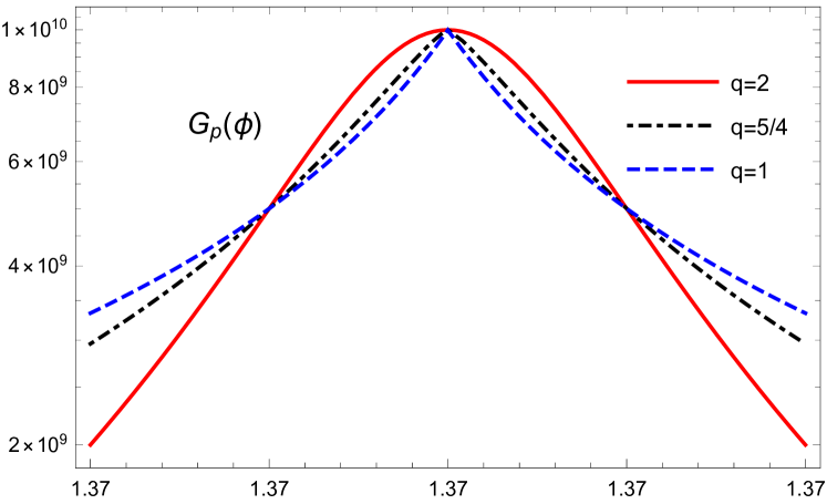
Figure 1: The peak function $G_{p}(\phi)$ with different $q$.

In summary, in our mechanism, the predictions for $n_{s}$ and $r$ are determined by the effective potential $U(\Phi)$ and the original potential in the action (1) is not restricted to a special form because the function $f(\phi)$ can reshape it to the effective potential; the shape of the enhanced power spectrum is controlled by $q$ in the peak function. In the next sections, we apply this mechanism to Higgs model and T-model.

III Higgs model

In this section, we show that the Higgs field can not only drive inflation but also explain DM in our universe in terms of PBH. The Higgs potential is

$$V(\phi)=\frac{\lambda}{4}\phi^{4},$$ (39)

where the coupling constant $\lambda\approx 0.13$ [104]. To obtain the predictions consistent with the observational constraints, we consider the effective potential $U(\phi)=U_{0}\Phi^{n}$ with $n=1/3$ and $n=2/3$, other values of $n$ such as $n=2/5$ and other forms of $U(\Phi)$ are also possible. Substituting the Higgs potential (39) into Eq. (36), we obtain

$$f(\phi)=f_{0}\phi^{-2+8/n},$$ (40)

where

$$f_{0}=\frac{16}{n^{2}}\left(\frac{\lambda}{4U_{0}}\right)^{2/n}.$$ (41)

For $n=1/3$, we get $f(\phi)=f_{0}\phi^{22}$. For $n=2/3$, we get $f(\phi)=f_{0}\phi^{10}$. At low energy scales $\phi\ll 1$, $f(\phi)$ is negligible and the model reduces to the standard case with the canonical kinetic term.

As mentioned above, the peak shape of the enhanced power spectrum is determined by $q$ in the peak function (38). To obtain different shapes of peak in the power spectrum, we consider the peak function (38) with $q=1$ and $q=5/4$ to demonstrate the sharp and broad peaks. To distinguish different models, as shown in Table 1, we label the model with $n=1/3$ and $q=1$ as H11, the model with $n=1/3$ and $q=5/4$ as H12, the model with $n=2/3$ and $q=1$ as H21, and the model with $n=2/3$ and $q=5/4$ as H22, respectively.

Label	$U(\phi)=U_{0}\Phi^{n}$	$q$
H11	$n=1/3$	$q=1$
H12	$n=1/3$	$q=5/4$
H21	$n=2/3$	$q=1$
H22	$n=2/3$	$q=5/4$

Table 1: The labeling for the Higgs models with different peak functions and effective potentials.

Choosing the value $\phi_{*}$ of the scalar field at the pivotal scale, the parameters $f_{0}$, $h$, $w$ and $\phi_{p}$ in the peak function as shown in Table 2, we numerically solve the background equations (2)-(4) and the perturbation equation

$$\frac{d^{2}u_{k}}{d\eta^{2}}+\left(k^{2}-\frac{1}{z}\frac{d^{2}z}{d\eta^{2}}\right)u_{k}=0,$$ (42)

to obtain the scalar power spectrum $\mathcal{P}_{\zeta}=k^{3}|\zeta_{k}|^{2}/(2\pi^{2})$, where the conformal time $\eta=\int dt/a(t)$, $u_{k}=z\zeta_{k}$ and $z=a\dot{\phi}(1+G)^{1/2}/H$. In Fig. 2, we show the results of the power spectra for the models H11 and H12 with blue and black lines respectively. The results for the models H21 and H22 are similar, so we don’t show them in the figures. From Fig. 2, we see that the power spectrum produced in the model H11 has a sharp peak while the power spectrum produced in the model H12 has a broad peak. Therefore, we can adjust the peak shape by choosing $q$. Additionally, the peak position or the scale where the power spectrum is enhanced can be adjusted by the parameter $\phi_{p}$ as shown in Table 2 and Fig. 2. To distinguish the scale for the enhanced power spectrum, we use additional labels “w,” “e,” and “s” as shown in Table 2. We also numerically calculate the scalar spectral index $n_{s}$ and the tensor-to-scalar ratio $r$ for these models and the results are shown in Table 2. As expected, the peak function has little influence on $n_{s}$ and $r$, and $n_{s}$ and $r$ are determined by the effective potential. For the models H11 and H12, we get

$$n_{s}\approx 0.967,\quad r\approx 0.040.$$ (43)

These results are consistent with the observational constraints and the slow-roll predictions (28). If $f_{0}$ is fixed as $f_{0}=1$ and the coupling constant $\lambda$ is chosen as $\lambda\sim 10^{-9}$, then similar power spectrum can be obtained [58]. When the running of Higgs self-coupling via the renormalization group equation is considered, $\lambda(\phi)=\lambda_{0}+b_{0}\ln^{2}(\phi/\mu)$, it was shown that the results keep to be almost the same [58]. Therefore, the mechanism is not sensitive to the choices of model parameters.

Model	$h$	$w$	$\phi_{p}/10^{-2}$	$\phi_{*}/10^{-2}$	$f_{0}$	$N$	$n_{s}$	$r$	$k_{\text{peak}}/\text{Mpc}^{-1}$
H11w	$1.56\times 10^{16}$	$1.12\times 10^{-14}$	$1.31$	$1.38$	$1.42\times 10^{48}$	$56$	$0.968$	$0.038$	$2.66\times 10^{12}$
H12w	$2.713\times 10^{17}$	$3.61\times 10^{-14}$	$1.284$	$1.4$	$9.60\times 10^{47}$	$66$	$0.965$	$0.041$	$2.26\times 10^{12}$
H11e	$1.415\times 10^{16}$	$1.18\times 10^{-14}$	$1.356$	$1.4$	$9.46\times 10^{47}$	$53$	$0.967$	$0.040$	$1.56\times 10^{9}$
H12e	$7.77\times 10^{16}$	$7.70\times 10^{-14}$	$1.325$	$1.38$	$1.42\times 10^{48}$	$61$	$0.967$	$0.039$	$1.71\times 10^{8}$
H11s	$1.47\times 10^{15}$	$1.128\times 10^{-13}$	$1.381$	$1.4$	$9.11\times 10^{47}$	$52$	$0.970$	$0.041$	$2.86\times 10^{5}$
H12s	$1.79\times 10^{17}$	$3.51\times 10^{-14}$	$1.354$	$1.38$	$1.42\times 10^{48}$	$60$	$0.967$	$0.039$	$2.56\times 10^{5}$
H11wf	$1.56\times 10^{16}$	$1.12\times 10^{-14}$	$1.31$	$1.38$	$1.42\times 10^{48}$	$56$	$0.968$	$0.038$	$2.55\times 10^{12}$
H21w	$9.147\times 10^{13}$	$1.841\times 10^{-12}$	$1.47$	$1.61$	$5.51\times 10^{24}$	$59$	$0.964$	$0.075$	$4.05\times 10^{12}$
H22w	$2.526\times 10^{17}$	$3.709\times 10^{-14}$	$1.416$	$1.62$	$5.29\times 10^{24}$	$68$	$0.964$	$0.074$	$4.50\times 10^{12}$
H21e	$8.70\times 10^{13}$	$1.81\times 10^{-12}$	$1.535$	$1.61$	$5.69\times 10^{24}$	$59$	$0.967$	$0.072$	$1.18\times 10^{9}$
H22e	$2.705\times 10^{16}$	$1.83\times 10^{-13}$	$1.51$	$1.62$	$5.28\times 10^{24}$	$63$	$0.964$	$0.074$	$9.57\times 10^{8}$
H21s	$8.70\times 10^{13}$	$1.78\times 10^{-12}$	$1.578$	$1.61$	$5.51\times 10^{24}$	$58$	$0.972$	$0.072$	$2.55\times 10^{5}$
H22s	$2.70\times 10^{16}$	$1.657\times 10^{-13}$	$1.562$	$1.62$	$5.28\times 10^{24}$	$62$	$0.964$	$0.073$	$3.56\times 10^{5}$

Table 2: The chosen parameter sets and the predictions of $n_{s}$ and $r$ for the Higgs model.

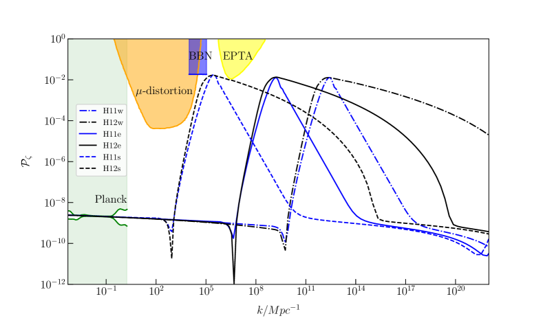
Figure 2: The enhanced power spectrum in the Higgs model. The blue and black lines denote the results for the models H11 with sharp peak and H12 with broad peak, respectively. The light green shaded region is excluded by the CMB observations [28]. The yellow, blue and orange regions show the constraints from the PTA observations [105], the effect on the ratio between neutron and proton during the big bang nucleosynthesis (BBN) [106] and $\mu$-distortion of CMB [107], respectively.

When the primordial curvature perturbation reenters the horizon during radiation dominated epoch, if the energy density contrast is large enough, it may gravitationally collapse to form PBHs. The parameter to describe the abundance of PBHs is the current fractional energy density of PBHs with the mass $M$ to DM which is derived in Appendix A in detail, and it is [20, 29]

$$\begin{split}Y_{\text{PBH}}(M)=&\frac{\beta(M)}{3.94\times 10^{-9}}\left(\frac{\gamma}{0.2}\right)^{1/2}\left(\frac{g_{*}}{10.75}\right)^{-1/4}\\ &\times\left(\frac{0.12}{\Omega_{\text{DM}}h^{2}}\right)\left(\frac{M}{M_{\odot}}\right)^{-1/2},\end{split}$$ (44)

where $M_{\odot}$ is the solar mass, $\gamma=0.2$ [108], $g_{*}$ is the effective degrees of freedom at the formation time, $\Omega_{\text{DM}}$ is the current energy density parameter of DM and $\Omega_{\text{DM}}h^{2}=0.12$ [109]; the fractional energy density of PBHs at the formation related to the power spectrum is [110, 111, 112]

$$\beta(M)\approx\sqrt{\frac{2}{\pi}}\frac{\sqrt{\mathcal{P}_{\zeta}}}{\mu_{c}}\exp\left(-\frac{\mu_{c}^{2}}{2\mathcal{P}_{\zeta}}\right),$$ (45)

with $\mu_{c}=9\delta_{c}/2\sqrt{2}$ and the threshold of the density perturbation for the PBH formation $\delta_{c}=0.4$ [113, 114, 112, 115, 116]. The value of $\delta_{c}$ may become larger by a factor of two if the non linearities between the Gaussian curvature perturbation and the density contrast and the nonlinear effects arising at horizon crossing are considered [117, 118]. Furthermore, the abundance of PBHs depends on the shape and non-Gaussianity of $\mathcal{P}_{\zeta}$ and nonlinear statistics need to be taken into account [119, 120, 121]. It was shown in Ref. [122] that non-Gaussianities of Higgs fluctuations are small at both the CMB and peak scales, so the effect of non-Gaussianities in the model is negligible. Combining Eq. (44) and Eq. (45), and using the numerical results of the power spectra for the models in Table 2 and Fig. 2, we obtain the abundance of PBHs for the corresponding models, and the results are shown in Fig. 3. The mass scale and the peak abundance of PBHs are shown in Table 3.

Figure 3: The abundances of PBHs produced in the models H11 and H12. The blue and black lines denote the results for the models H11 and H12, respectively. The shaded regions show the observational constraints on the PBH abundance: the yellow region from accretion constraints by CMB [123, 124], the red region from extragalactic gamma-rays by PBH evaporation (EG$\gamma$) [125], the cyan region from galactic center 511 keV gamma-ray line (INTEGRAL) [126, 127, 128], the orange region from white dwarf explosion (WD) [129], the green region from microlensing events with Subaru HSC [130], the blue region from the Kepler satellite [131], the gray region from the EROS/MACHO [132].

From Figs. 2 and 3, we see that different peak scales correspond to different peak masses of PBHs. A broad peak in the primordial scalar power spectrum produces a broad peak in $Y_{\text{PBH}}$. The models with the label “w” produce PBHs with the mass around $10^{-14}-10^{-12}M_{\odot}$, the models with the label “e” produce PBHs with the Earth’s mass, the models with the label “s” produce PBHs with the stellar mass. The PBHs with masses around $10^{-14}-10^{-12}M_{\odot}$ almost make up all the DM and the peak abundances of them are about $Y_{\text{PBH}}^{\text{peak}}\approx 1$. Therefore, the Higgs field not only drives inflation but also explains DM. In our models H11e, H12e, H21e and H22e, we successfully produce PBHs with the mass around $\mathcal{O}(1)M_{\oplus}$ which could be used to explain the origin of the Planet 9. PBHs with the stellar mass which explain the LIGO events are also produced in the Higgs model.

Model	$\mathcal{P}_{\zeta(\text{peak})}$	$M_{\text{peak}}/M_{\odot}$	$Y_{\text{PBH}}^{\text{peak}}$	$f_{c}/\text{Hz}$
H11w	$0.0128$	$5.22\times 10^{-13}$	$0.70$	$4.30\times 10^{-3}$
H12w	$0.0129$	$7.22\times 10^{-13}$	$0.73$	$4.01\times 10^{-3}$
H11e	$0.0126$	$1.51\times 10^{-6}$	$2.38\times 10^{-4}$	$2.70\times 10^{-6}$
H12e	$0.0134$	$1.26\times 10^{-6}$	$1.92\times 10^{-3}$	$2.90\times 10^{-6}$
H11s	$0.0178$	$45.1$	$5.72\times 10^{-4}$	$4.82\times 10^{-10}$
H12s	$0.0167$	$50.8$	$1.22\times 10^{-4}$	$4.37\times 10^{-10}$
H11wf	$0.0129$	$5.65\times 10^{-13}$	$0.78$	$4.61\times 10^{-3}$
H21w	$0.0128$	$2.24\times 10^{-13}$	$0.97$	$6.64\times 10^{-3}$
H22w	$0.0126$	$1.82\times 10^{-13}$	$0.63$	$6.96\times 10^{-3}$
H21e	$0.0131$	$2.66\times 10^{-6}$	$6.37\times 10^{-4}$	$2.03\times 10^{-6}$
H22e	$0.0120$	$4.02\times 10^{-6}$	$2.55\times 10^{-5}$	$1.48\times 10^{-6}$
H21s	$0.0176$	$56.5$	$3.97\times 10^{-4}$	$6.69\times 10^{-10}$
H22s	$0.0173$	$21.9$	$4.01\times 10^{-4}$	$6.33\times 10^{-10}$

Table 3: The results for the peak amplitude of the primordial scalar power spectrum, the peak mass and abundance of PBHs and the peak frequency of SIGWs with the chosen parameter sets shown in Table 2.

Accompanied by the production of PBHs, the large scalar perturbations induce GWs during radiation. These SIGWs consist of the stochastic background, and they could be detected by the space based GW detectors like LISA [93, 94], Taiji [95] and TianQin [96] in the future and provide additional constraints on the primordial Universe. We present the energy density of SIGWs in the radiation domination in detail in the Appendix B, and it is [72, 77]

$$\begin{split}\Omega_{\mathrm{GW}}(k,\eta)=&\frac{1}{6}\left(\frac{k}{aH}\right)^{2}\int_{0}^{\infty}dv\int_{|1-v|}^{1+v}du\\ &\left[\frac{4v^{2}-(1-u^{2}+v^{2})^{2}}{4uv}\right]^{2}\\ &\times\overline{I_{\text{RD}}^{2}(u,v,x)}\mathcal{P}_{\zeta}(kv)\mathcal{P}_{\zeta}(ku),\end{split}$$ (46)

where $I_{\text{RD}}$ is defined in Eq. (91). Substituting the numerical results for the power spectra of the models listed in Table 2 into Eq. (46), we obtain the energy density $\Omega_{\text{GW}}$ of SIGWs for the corresponding models and the results are shown in Fig. 4. The peak frequencies $f_{c}$ of these SIGWs are shown in Table 3. From Table 3, we see that the peak frequencies of the SIGWs are around mHz, $10^{-6}$Hz and nHz respectively. For the models H11 and H21, both $\mathcal{P}_{\zeta}$ and $\Omega_{\text{GW}}$ have sharp peaks. The mHz and nHz SIGWs may be detected by LISA/Taiji/TianQin and PTA respectively. For the models H12 and H22, the enhanced $\mathcal{P}_{\zeta}$ has half-domed shape and $\Omega_{\text{GW}}$ has a broad shape which spans a wide frequency bands. The models H12s and H22s which produce the stellar mass PBHs and have a broad shape for $\Omega_{\text{GW}}$ are excluded by the EPTA data [88, 89, 90, 91], while the models H11s and H21s generating SIGWs with a sharp peak can be tested by SKA [92]. The models H11w, H12w, H12e, H21w, H22w and H22e can be tested by LISA/Taiji/TianQin. However, the models H11e and H21e which generate SIGWs with a sharp peak is beyond the reach of either SKA or LISA/Taiji/TianQin.

From the point of view of the effective field theory, the lower dimensional terms in $f(\phi)$ need to be taken into account, i.e., we need to consider $f(\phi)=f_{0}\phi^{22}+\delta f$ with $\delta f=\sum_{n=4}^{21}C_{n}\phi^{n}$ and $C_{n}<O(1)$. To consider the effects of the lower dimensional terms of $f(\phi)$, we choose $\delta f=\sum_{n=4}^{21}\phi^{n}$ and as an example we apply the correction $\delta f$ to the model H11w. The model with the correction $\delta f$ in $f(\phi)$ is called H11wf. We choose the same parameters for the models H11w and H11wf and the results are shown in Tables 2 and 3. From Tables 2 and 3, we see that the results for the models H11wf and H11w are almost the same. Therefore, the lower dimensional terms have little effect on the enhancement mechanism and the correction $\delta f$ does not spoil the enhancement mechanism.

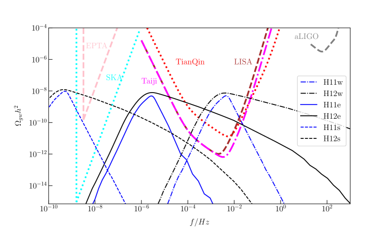
Figure 4: The scalar induced secondary GWs for the Higgs model. The blue and black lines denote the models H11 and H12, respectively. The pink dashed curve denotes the EPTA limit [88, 89, 90, 91] , the cyan dotted curve denotes the SKA limit [92], the red dot-dashed curve in the middle denotes the TianQin limit [96], the dotted magenta curve shows the Taiji limit [95], the brown dashed curve shows the LISA limit [94], and the gray dot-dashed curve denotes the aLIGO limit [133, 134].

IV T-model

T-model with the canonical kinetic term is consistent with the observational constraints. In this section, we show that our mechanism works for T-model too, henceforth show that the inflationary potential in our mechanism is not restricted. The potential for T-model is [135, 136, 137]

$$V(\phi)=V_{0}\tanh^{2m}\left(\frac{\phi}{\sqrt{6\alpha}}\right).$$ (47)

Substituting the potential (47) into Eq. (36), we obtain

$$f(\phi)=f_{0}~{}\text{sech}^{4}\left(\frac{\phi}{\sqrt{6\alpha}}\right)\tanh^{-2+4m/n}\left(\frac{\phi}{\sqrt{6\alpha}}\right),$$ (48)

where

$$f_{0}=\frac{2}{3\alpha}\left(\frac{V_{0}}{U_{0}}\right)^{2/n}\frac{m^{2}}{n^{2}}.$$ (49)

For the parameters considered in this section, we take $f_{0}=36$. For $n=1/3$, we obtain

$$f(\phi)=36\text{sech}^{4}\left(\frac{\phi}{\sqrt{6\alpha}}\right)\tanh^{12m-2}\left(\frac{\phi}{\sqrt{6\alpha}}\right).$$ (50)

For $n=2/3$, we obtain

$$f(\phi)=36\text{sech}^{4}\left(\frac{\phi}{\sqrt{6\alpha}}\right)\tanh^{6m-2}\left(\frac{\phi}{\sqrt{6\alpha}}\right).$$ (51)

Similar to the Higgs model, at low energy scales $\phi\ll 1$, $f(\phi)$ is negligible and the model reduces to the standard case with the canonical kinetic term.

As discussed above, the peak shape of the enhanced power spectrum is determined by $q$ in the peak function (38). Similar to the Higgs model, we also consider the peak function (38) with $q=1$ and $q=5/4$ to explore the sharp and broad peaks. To distinguish different models, as shown in Table 4, the model with $m=1/6$, $\alpha=1$ and $n=1/3$ is labeled as T1 and the model with $m=1/3$, $\alpha=1$ and $n=2/3$ is labeled as T2. Additionally, we label the model with $n=1/3$ and $q=1$ as T11, the model with $n=1/3$ and $q=5/4$ as T12, the model with $n=2/3$ and $q=1$ as T21, and the model with $n=2/3$ and $q=5/4$ as T22, respectively.

Label	$U(\phi)=U_{0}\Phi^{n}$	$q$
T11	$n=1/3$	$q=1$
T12	$n=1/3$	$q=5/4$
T21	$n=2/3$	$q=1$
T22	$n=2/3$	$q=5/4$

Table 4: The labeling for the T-models with different peak functions and effective potentials.

Choosing the parameter $V_{0}$, the value $\phi_{*}$ of the scalar field at the pivotal scale, and the parameters $h$, $w$ and $\phi_{p}$ in the peak function as shown in Table 5, we numerically solve the background equations (2)-(4) and the perturbation equation (42) to obtain the scalar power spectrum and the results are shown in Fig. 5. The power spectra for the models T11 and T12 are denoted by blue and black lines respectively. The results for the models T21 and T22 are similar with those of T11 and T12, so we do not show them in the figures. The power spectrum produced in the model T11 has a sharp peak while the power spectrum produced in the model T12 has a broad peak. This implies that the peak shape in the power spectrum is unaffected by the potential but affected by the peak function. The scale where the power spectrum is enhanced can be adjusted by the parameter $\phi_{p}$ and the results are shown in Table 5 and Fig 5. The numerical results for the scalar spectral index $n_{s}$ and the tensor-to-scalar ratio $r$ are shown in Table 5. For the models T11 and T12, we get

$$n_{s}\approx 0.968,\quad r\approx 0.038.$$ (52)

These results are similar to those for the Higgs models H11 and H12. As expected, $n_{s}$ and $r$ are almost unaffected by the peak function whose effect is negligible at large scales as well as the inflationary potential, and they are determined by the effective potential.

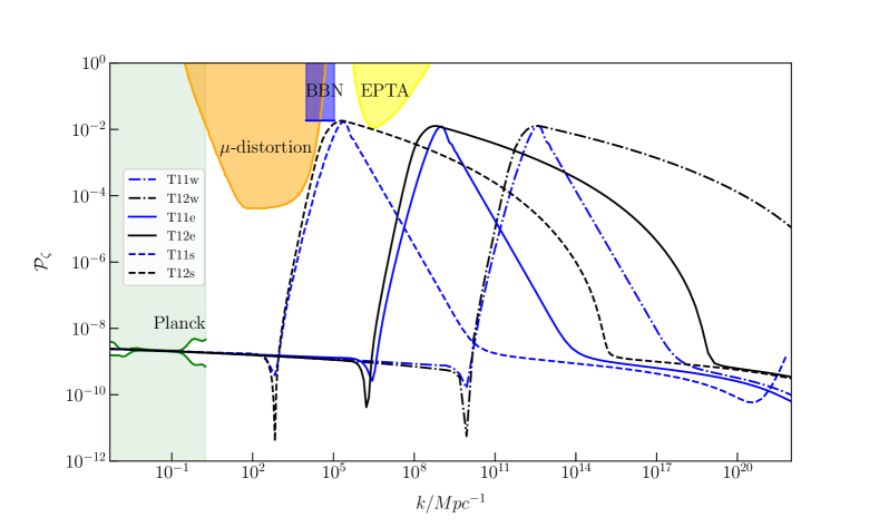
Figure 5: The enhanced power spectrum in the T-model. The blue and black lines denote the results for the models T11 with sharp peak and T12 with broad peak, respectively.

Model	$h$	$w$	$\phi_{p}$	$\phi_{*}$	$U_{0}/10^{-9}$	$N$	$n_{s}$	$r$	$k_{\text{peak}}/\text{Mpc}^{-1}$
T11w	$4.86\times 10^{9}$	$8.885\times 10^{-11}$	$0.44$	$0.81$	$1.67$	$56$	$0.969$	$0.037$	$4.01\times 10^{12}$
T12w	$2.109\times 10^{11}$	$8.481\times 10^{-11}$	$0.32$	$0.81$	$1.71$	$66$	$0.966$	$0.038$	$3.85\times 10^{12}$
T11e	$3.57\times 10^{9}$	$8.89\times 10^{-11}$	$0.58$	$0.81$	$1.65$	$55$	$0.969$	$0.037$	$1.01\times 10^{9}$
T12e	$1.139\times 10^{9}$	$8.68\times 10^{-11}$	$0.51$	$0.81$	$1.71$	$61$	$0.967$	$0.038$	$6.12\times 10^{8}$
T11s	$3.178\times 10^{9}$	$8.92\times 10^{-11}$	$0.644$	$0.76$	$1.84$	$51$	$0.970$	$0.040$	$2.31\times 10^{5}$
T12s	$8.633\times 10^{9}$	$8.56\times 10^{-11}$	$0.642$	$0.81$	$1.70$	$60$	$0.967$	$0.038$	$2.00\times 10^{5}$
T21w	$9.205\times 10^{9}$	$4.85\times 10^{-11}$	$0.80$	$1.31$	$3.07$	$61$	$0.969$	$0.063$	$3.02\times 10^{12}$
T22w	$4.51\times 10^{11}$	$4.644\times 10^{-11}$	$0.63$	$1.30$	$3.23$	$70$	$0.967$	$0.066$	$5.47\times 10^{12}$
T21e	$8.34\times 10^{9}$	$4.17\times 10^{-11}$	$0.98$	$1.31$	$3.04$	$61$	$0.970$	$0.062$	$8.20\times 10^{8}$
T22e	$2.33\times 10^{11}$	$5.54\times 10^{-11}$	$0.88$	$1.31$	$3.17$	$66$	$0.967$	$0.065$	$7.97\times 10^{8}$
T21s	$7.00\times 10^{9}$	$4.11\times 10^{-11}$	$1.14$	$1.31$	$2.97$	$60$	$0.974$	$0.061$	$2.73\times 10^{5}$
T22s	$2.20\times 10^{11}$	$4.74\times 10^{-11}$	$1.06$	$1.31$	$3.16$	$65$	$0.967$	$0.065$	$2.31\times 10^{5}$

Table 5: The chosen parameter sets and the predictions of $n_{s}$ and $r$ for the T-model.

Using the numerical results of the power spectra for the models as shown in Fig. 5 and combining them with Eq. (44), we obtain the abundances of PBHs and the results are shown in Fig. 6. The peak mass and the abundance of PBHs are shown in Table 6. The models labeled as “w” produce PBHs with the mass around $10^{-14}-10^{-12}M_{\odot}$ and the peak abundance $Y_{\text{PBH}}^{\text{peak}}\approx 1$, which make up almost all the DM. The models labeled as “e” produce PBHs with the mass around $\mathcal{O}(1)M_{\oplus}$, which can be used to explain the origin of the Planet 9. The models labeled as “s” produce PBHs with the stellar mass that may account for the LIGO events. Therefore, in our mechanism, T-model can also produce PBHs with different mass and explain DM in terms of PBHs.

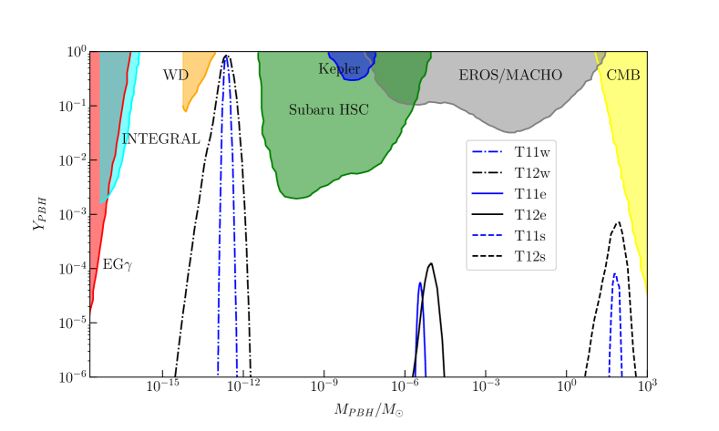
Figure 6: The PBHs abundance for the models display in Fig. 5. The blue and black lines denote the models labeled as T11, T12, respectively.

Model	$\mathcal{P}_{\zeta(\text{peak})}$	$M_{\text{peak}}/M_{\odot}$	$Y_{\text{PBH}}^{\text{peak}}$	$f_{c}/\text{Hz}$
T11w	$0.0127$	$2.28\times 10^{-13}$	$0.83$	$7.03\times 10^{-3}$
T12w	$0.0128$	$2.48\times 10^{-13}$	$0.88$	$6.54\times 10^{-3}$
T11e	$0.0122$	$3.67\times 10^{-6}$	$5.51\times 10^{-5}$	$1.70\times 10^{-6}$
T12e	$0.0127$	$9.04\times 10^{-6}$	$1.24\times 10^{-4}$	$1.07\times 10^{-6}$
T11s	$0.0165$	$59.97$	$8.00\times 10^{-5}$	$3.83\times 10^{-10}$
T12s	$0.0183$	$91.75$	$7.12\times 10^{-4}$	$3.48\times 10^{-10}$
T21w	$0.0128$	$4.03\times 10^{-13}$	$0.77$	$5.06\times 10^{-3}$
T22w	$0.0125$	$9.71\times 10^{-14}$	$0.58$	$9.91\times 10^{-3}$
T21e	$0.0127$	$5.47\times 10^{-6}$	$1.35\times 10^{-4}$	$1.43\times 10^{-6}$
T22e	$0.0126$	$5.79\times 10^{-6}$	$1.21\times 10^{-4}$	$3.21\times 10^{-6}$
T21s	$0.0166$	$49.4$	$9.73\times 10^{-5}$	$5.10\times 10^{-10}$
T22s	$0.0174$	$45.4$	$3.10\times 10^{-4}$	$4.40\times 10^{-10}$

Table 6: The results for the peak amplitude of the primordial scalar power spectrum, the peak mass and abundance of PBH and the peak frequency of SIGWs with the chosen parameter sets shown in Table 5.

Combining the numerical results of the power spectra as shown in Fig. 5 and Eq. (46), we obtain the energy density $\Omega_{\text{GW}}$ of SIGWs and the results are shown in Fig. 7. The results are similar to those in the Higgs model. The peak frequencies of these SIGWs are shown in Table 6. The SIGWs have a sharp peak in the models T11 and have a broad peak in the models T12. The scalar perturbations producing PBHs with the mass around $10^{-14}-10^{-12}M_{\odot}$ generate SIGWs with the frequency around mHz which can be detected by LISA/Taiji/TianQin. The scalar perturbations producing PBHs with the mass around $M_{\oplus}$ generate SIGWs with the frequency around $10^{-6}$Hz. The SIGWs with a broad peak may be detected by LISA/Taiji/TianQin, but the SIGWs with a sharp peak is beyond the reach of either SKA or LISA/Taiji/TianQin. The scalar perturbations producing PBHs with the stellar mass generate SIGWs with the frequency around nHz. The SIGWs with a broad peak are excluded by the EPTA data and the SIGWs with a sharp peak can be tested by SKA.

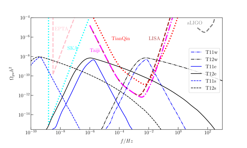
Figure 7: The SIGWs for the T-model. The blue and black lines denote the models T11 and T12, respectively.

V conclusion

In the standard case that the inflaton has the canonical kinetic term and is minimally coupled to gravity, Higgs field as the inflaton is excluded by the CMB constraints because the amplitude of the primordial GWs produced in Higgs model is too large. By introducing a noncanonical kinetic term with a peak, the amplitude of the primordial GWs produced in Higgs model at large scales is successfully reduced and the inflation driven by the Higgs field is consistent with Planck 2018 results. The scalar power spectrum is also enhanced at small scales. The enhanced curvature perturbations at small scales produce abundant PBH DM and generate SIGWs after the horizon reentry during radiation domination. The peak scale at which the scalar power spectrum is enhanced can be easily adjusted. As examples, we use three different parameter sets to show how to get the enhanced power spectra at three different scales. With these enhanced power spectra, PBHs with the peak mass around $10^{-14}-10^{-12}M_{\odot}$, the Earth’s mass and the stellar mass are produced respectively. The corresponding peak abundances are $Y_{\text{PBH}}\sim 1$, $Y_{\text{PBH}}\sim 10^{-4}$ and $Y_{\text{PBH}}\sim 10^{-4}$. Therefore, PBHs with the peak mass around $10^{-14}-10^{-12}M_{\odot}$ can explain almost all the DM. At the same time, the SIGWs with the peak frequency around mHz, $10^{-6}$Hz and nHz are generated. Dependent on the peak function, the peak shape of the enhanced power spectrum can be sharp or broad which is like half domed, and the peak shape of the energy density of the SIGWs can be also sharp or broad. The SIGWs with broad peaks and peak frequency around nHz are excluded by the EPTA observations. In general, the SIGWs can be tested by PTA observations and space based GW detectors.

The scalar spectral index $n_{s}$ and the tensor-to-scalar ratio $r$ predicated in the T-model with the canonical kinetic term are consistent with Planck 2018 results. We also show that the enhancement mechanism works for the T-model and the results for the T-model are similar to those for the Higgs model.

In conclusion, with the enhancement mechanism provided by the noncanonical kinetic term with a peak, the Higgs field accounts for the origin of mass and DM in terms of PBHs, the SIGWs can be tested by PTA observations and the space based GW detectors. In addition to the Higgs field, the enhancement mechanism also works for T-model and other inflationary potentials. The energy density of the SIGWs can have sharp or broad peaks. Both the GW and PBH observations can be used to test this mechanism and probe physics in the early universe.

Appendix A THE PRIMORDIAL BLACK HOLES

The stellar mass PBHs could be those detected by LIGO/Virgo collaboration and they can also explain DM, even make up all the DM with the mass in the windows $10^{-17}-10^{-15}M_{\odot}$ and $10^{-14}-10^{-12}M_{\odot}$. In this appendix, we briefly review the formulas about the production of PBHs. The energy density fraction of PBHs at formation to the total mass of the Universe is

$$\beta=\left.\frac{\rho_{\text{PBH}}}{\rho}\right|_{\text{at formation}},$$ (53)

where $\rho$ is the energy density of the Universe and $\rho_{\text{PBH}}$ is the energy density of PBHs. The relation between the energy density of PBHs at the formation and that at present is

$$\rho_{\text{PBH}}=\left(\frac{a_{0}}{a}\right)^{3}\frac{3H_{0}^{2}}{8\pi G}~{}\Omega_{\text{PBH}_{0}},$$ (54)

where the subscript ‘$0$’ denotes the present value of a quantity and $\Omega_{\text{PBH}}=8\pi G\rho_{\text{PBH}}/3H^{2}$ is the density parameter of PBHs. The relation between the energy density of the radiation $\rho_{r}$ and temperature $T$ is

$$\rho_{r}=\frac{\pi^{2}}{30}g_{*}T^{4},$$ (55)

where $g_{*}$ is the number of relativistic degrees of freedom. Assuming the entropy is conserved, we have

$$S=g_{*s}a^{3}T^{3}=\text{constant},$$ (56)

where $g_{*s}$ is the number of entropy degrees of freedom which is approximately equal to the number of relativistic degrees of freedom, $g_{*s}=g_{*}$. Combining the above equations with the Friedmann equation of the Universe,

$$H^{2}=\frac{8\pi G}{3}\rho,$$ (57)

and assuming PBHs are formed during the radiation dominated epoch, we obtain the relation of Hubble parameter at formation to that at today

$$H^{2}=a^{-4}\left(\frac{g_{*}}{g_{*_{0}}}\right)^{-1/3}H_{0}^{2}\Omega_{r_{0}},$$ (58)

where we set $a_{0}=1$. Combining Eq. (57) with Eq. (58), and using the definition (53), we obtain

$$\beta=\left(\frac{H_{0}}{H}\right)^{1/2}\left(\frac{g_{*}}{g_{*_{0}}}\right)^{1/4}\Omega_{r_{0}}^{-3/4}\Omega_{\text{PBH}_{0}}.$$ (59)

The mass of the PBH could be assumed as

$$M_{\text{PBH}}=\gamma M_{H},$$ (60)

where $\gamma\approx 0.2$ [108] is determined by the detail of the formation of the PBH and $M_{H}$ is the total mass in the horizon at the PBH formation,

$$M_{H}=\frac{4\pi}{3}H^{-3}\rho=\frac{1}{2GH}.$$ (61)

At the peak scale $k_{\text{peak}}$, the peak mass of PBH is

$$M_{\text{peak}}=3.68\left(\frac{\gamma}{0.2}\right)\left(\frac{g_{*}}{10.75}\right)^{-1/6}\left(\frac{k_{\text{peak}}}{10^{6}\ \text{Mpc}^{-1}}\right)^{-2}M_{\odot}.$$ (62)

Combining Eq. (59) and Eq. (60), we obtain

$$\beta=\gamma^{-1/2}\left(\frac{M_{\text{PBH}}}{M_{0}}\right)^{1/2}\left(\frac{g_{*}}{g_{*_{0}}}\right)^{1/4}\Omega_{r_{0}}^{-3/4}\Omega_{\text{PBH}_{0}},$$ (63)

where $M_{0}=(2GH_{0})^{-1}$ is the horizon mass at the present. The definition for the current fractional energy density of PBHs with the mass $M$ to the DM is

$$Y_{\text{PBH}}=\frac{\Omega_{\text{PBH}_{0}}}{\Omega_{{\text{DM}_{0}}}}.$$ (64)

Substituting the definition (64) into (63), we obtain

$$\beta=\gamma^{-1/2}\left(\frac{M_{\text{PBH}}}{M_{0}}\right)^{1/2}\left(\frac{g_{*}}{g_{*_{0}}}\right)^{1/4}\Omega_{r_{0}}^{-3/4}\Omega_{\text{DM}_{0}}Y_{\text{PBH}}.$$ (65)

The PBHs would be formed if the density contrast of the overdense regions at horizon reentry during radiation domination exceeds a certain threshold value. In Press-Schechter theory, the fraction $\beta$ could be regarded as the probability that the density contrast exceeds the threshold $\delta_{c}=0.4$ [114],

$$\beta=2\int_{\delta_{c}}^{1}P(\delta(R))d\delta(R),$$ (66)

where $\delta(R)$ is the smoothed density contrast and $R=(aH)^{-1}$ is the smooth scale, $P(\delta(R))$ is the distribution of the smoothed overdensity. Assuming the Gaussian initial perturbations, the probability function for the smoothed density contrast is

$$P(\delta(R))=\frac{1}{\sqrt{2\pi}\sigma(R)}\exp\left(-\frac{\delta(R)^{2}}{2\sigma(R)^{2}}\right),$$ (67)

with the variance satisfying

$$\sigma(R)^{2}=\int_{0}^{\infty}W^{2}(kR)\frac{\mathcal{P}_{\delta}(k)}{k}dk,$$ (68)

where $\mathcal{P}_{\delta}$ is the power spectrum of the matter perturbation and $W(kR)$ is the window function. In our paper, we choose the Gaussian window function

$$W(kR)=\exp\left(-k^{2}R^{2}/2\right),$$ (69)

other kinds of window functions are also possible [138]. The relation between the matter perturbation and the primordial curvature perturbation is

$$\mathcal{P}_{\delta}(k)=\frac{4(1+w)^{2}}{(5+3w)^{2}}\left(\frac{k}{aH}\right)^{4}\mathcal{P}_{\zeta}(k).$$ (70)

Substituting the Gaussian window function (69) and Eq. (70) into Eq. (68), the mass variance becomes

$$\sigma^{2}=\frac{4(1+w)^{2}}{(5+3w)^{2}}\int_{0}^{\infty}x^{3}\exp\left(-x^{2}\right)\mathcal{P}_{\zeta}(x/R)dx,$$ (71)

where $x=kR$. As a suitable approximation, we assume the primordial curvature power spectrum is scale invariant even though it may change rapidly, because the integral (71) is dominated by the scale $x\sim 1$ and other scale has little influence on the result [31]. The mass variance (71) becomes

$$\sigma^{2}\approx\frac{2(1+w)^{2}}{(5+3w)^{2}}\mathcal{P}_{\zeta}(1/R).$$ (72)

Substituting Eq. (72) into the definition (66) and combining it with the probability function (67), we obtain

$$\begin{split}\beta&=\text{erfc}\left(\frac{5+3w}{2(1+w)}\frac{\delta_{c}}{\sqrt{\mathcal{P}_{\zeta}}}\right)\\ &\approx\sqrt{\frac{2}{\pi}}\frac{\sqrt{\mathcal{P}_{\zeta}}}{\mu_{c}}\exp\left(-\frac{\mu_{c}^{2}}{2\mathcal{P}_{\zeta}}\right),\end{split}$$ (73)

where $\text{erfc}(x)$ is the complementary error function, and

$$\mu_{c}=\frac{5+3w}{\sqrt{2}(1+w)}\delta_{c}.$$ (74)

Combining Eq. (65) and Eq. (73), we can predict the abundance of PBHs produced from the primordial curvature perturbations. Substituting $\Omega_{r_{0}}=9.17\times 10^{-5}$, $g_{*_{0}}=3.36$, $M_{0}\approx 4.63\times 10^{22}M_{\odot}$ and $H_{0}=67.27\text{km}/\text{s}/\text{Mpc}$ into Eq. (63), we obtain

$$\begin{split}Y_{\text{PBH}}(M)=&\frac{\beta(M)}{3.94\times 10^{-9}}\left(\frac{\gamma}{0.2}\right)^{1/2}\left(\frac{g_{*}}{10.75}\right)^{-1/4}\\ &\times\left(\frac{0.12}{\Omega_{\text{DM}}h^{2}}\right)\left(\frac{M}{M_{\odot}}\right)^{-1/2},\end{split}$$ (75)

where $M$ is the mass of the PBH.

Appendix B THE SCALAR INDUCED SECONDARY GRAVITATIONAL WAVES

Accompanied by the production of PBHs, the large scalar perturbations generate SIGWs during radiation domination. In this appendix, we review the generation of SIGWs in detail. The perturbed metric in the Newtonian gauge in the cosmological background is

$$\begin{split}ds^{2}=&-a^{2}(\eta)(1+2\Phi)d\eta^{2}+\\ &a^{2}(\eta)\left[(1-2\Phi)\delta_{ij}+\frac{1}{2}h_{ij}\right]dx^{i}dx^{j},\end{split}$$ (76)

where $\eta$ is the conformal time, $\Phi$ is the Bardeen potential, and we neglect the anisotropic stress. The Fourier transform of tensor perturbations $h_{ij}$ is

$$h_{ij}(\bm{x},\eta)=\frac{1}{(2\pi)^{3/2}}\int d^{3}ke^{i\bm{k}\cdot\bm{x}}[h_{\bm{k}}(\eta)e_{ij}(\bm{k})+\tilde{h}_{\bm{k}}(\eta)\tilde{e}_{ij}(\bm{k})],$$ (77)

where $e_{ij}(\bm{k})$ and $\tilde{e}_{ij}(\bm{k})$ are the plus and cross polarization tensors,

$$e_{ij}(\bm{k})=\frac{1}{\sqrt{2}}\left[e_{i}(\bm{k})e_{j}(\bm{k})-\tilde{e}_{i}(\bm{k})\tilde{e}_{j}(\bm{k})\right],$$ (78)

$$\tilde{e}_{ij}(\bm{k})=\frac{1}{\sqrt{2}}\left[e_{i}(\bm{k})\tilde{e}_{j}(\bm{k})+\tilde{e}_{i}(\bm{k})e_{j}(\bm{k})\right],$$ (79)

and the orthonormal basis vectors $\bm{e}$ and $\tilde{\bm{e}}$ are orthogonal to $\bm{k}$, satisfying $\bm{e}\cdot\tilde{\bm{e}}=\bm{e}\cdot\bm{k}=\tilde{\bm{e}}\cdot\bm{k}$. The equation for the Fourier component of the tensor perturbation with either polarization induced by the scalar perturbation is [62, 63]

$$h^{\prime\prime}_{\bm{k}}+2\mathcal{H}h^{\prime}_{\bm{k}}+k^{2}h_{\bm{k}}=4S_{\bm{k}},$$ (80)

where a prime denotes the derivative with respect to the conformal time, $h^{\prime}_{\bm{k}}=dh_{\bm{k}}/d\eta$, $\mathcal{H}=a^{\prime}/a$ is the conformal Hubble parameter, the scalar source is

$$\begin{split}S_{\bm{k}}=&\int\frac{d^{3}\tilde{k}}{(2\pi)^{3/2}}e_{ij}(\bm{k})\tilde{k}^{i}\tilde{k}^{j}\left[2\Phi_{\tilde{\bm{k}}}\Phi_{\bm{k}-\tilde{\bm{k}}}\phantom{\frac{1}{2}}+\right.\\ &\left.\frac{1}{\mathcal{H}^{2}}\left(\Phi^{\prime}_{\tilde{\bm{k}}}+\mathcal{H}\Phi_{\tilde{\bm{k}}}\right)\left(\Phi^{\prime}_{\bm{k}-\tilde{\bm{k}}}+\mathcal{H}\Phi_{\bm{k}-\tilde{\bm{k}}}\right)\right],\end{split}$$ (81)

$\Phi_{k}$ is the Fourier component of the Bardeen potential, and it can be related with its primordial value $\phi_{\bm{k}}$ by the transfer function

$$\Phi_{\bm{k}}=\Psi(k\eta)\phi_{\bm{k}}.$$ (82)

The transfer function $\Psi$ in the radiation domination is

$$\Psi(x)=\frac{9}{x^{2}}\left[\frac{\sin(x/\sqrt{3})}{x/\sqrt{3}}-\cos(x/\sqrt{3})\right].$$ (83)

The primordial value $\phi_{k}$ relating to the primordial scalar power spectrum $\mathcal{P}_{\zeta}$ produced during inflation is

$$\langle\phi_{\bm{k}}\phi_{\tilde{\bm{k}}}\rangle=\delta^{(3)}(\bm{k}+\tilde{\bm{k}})\frac{2\pi^{2}}{k^{3}}\left(\frac{3+3w}{5+3w}\right)^{2}\mathcal{P}_{\zeta}(k),$$ (84)

where $w$ is the equation of state of matter in the Universe determined by the time when the perturbations reenter the horizon. The definition of the power spectrum $\mathcal{P}_{h}(k,\eta)$ for the SIGWs is

$$\langle h_{\bm{k}}(\eta)h_{\tilde{\bm{k}}}(\eta)\rangle=\frac{2\pi^{2}}{k^{3}}\delta^{(3)}(\bm{k}+\tilde{\bm{k}})\mathcal{P}_{h}(k,\eta),$$ (85)

and the fractional energy density is

$$\Omega_{\mathrm{GW}}(k,\eta)=\frac{1}{24}\left(\frac{k}{aH}\right)^{2}\overline{\mathcal{P}_{h}(k,\eta)}.$$ (86)

We solve the tensor equation (80) by the Green function method, and the solution is

$$h_{k}(\eta)=\frac{4}{a(\eta)}\int_{\eta_{k}}^{\eta}d\tilde{\eta}g_{k}(\eta,\tilde{\eta})a(\tilde{\eta})S_{k}(\tilde{\eta}),$$ (87)

where the corresponding Green function is

$$g_{k}(\eta,\eta^{\prime})=\frac{\sin\left[k(\eta-\eta^{\prime})\right]}{k}.$$ (88)

Substituting the solution (87) into Eq. (85), we obtain the power spectrum for the SIGWs [63, 62, 77, 78]

$$\begin{split}\mathcal{P}_{h}(k,\eta)=&4\int_{0}^{\infty}dv\int_{|1-v|}^{1+v}du\left[\frac{4v^{2}-(1-u^{2}+v^{2})^{2}}{4uv}\right]^{2}\\ &\times I_{RD}^{2}(u,v,x)\mathcal{P}_{\zeta}(kv)\mathcal{P}_{\zeta}(ku),\end{split}$$ (89)

Using the definition of the fractional energy density, we obtain

$$\begin{split}\Omega_{\mathrm{GW}}(k,\eta)=&\frac{1}{6}\left(\frac{k}{aH}\right)^{2}\int_{0}^{\infty}dv\int_{|1-v|}^{1+v}du\\ &\times\left[\frac{4v^{2}-(1-u^{2}+v^{2})^{2}}{4uv}\right]^{2}\\ &\times\overline{I_{\text{RD}}^{2}(u,v,x)}\mathcal{P}_{\zeta}(kv)\mathcal{P}_{\zeta}(ku),\end{split}$$ (90)

where $u=|\bm{k}-\tilde{\bm{k}}|/k$, $v=\tilde{k}/k$, $x=k\eta$ and the integral kernel $I_{\text{RD}}$ is [78, 30]

$$\begin{split}I_{\text{RD}}(u,v,x)=&\int_{1}^{x}dy\,y\sin(x-y)\{3\Psi(uy)\Psi(vy)\\ &+y[\Psi(vy)u\Psi^{\prime}(uy)+v\Psi^{\prime}(vy)\Psi(uy)]\\ &+y^{2}uv\Psi^{\prime}(uy)\Psi^{\prime}(vy)\}.\end{split}$$ (91)

This integral kernel can split into two parts, one is the sine part and the other is the cosine part,

$$I_{\text{RD}}(u,v,x)=\frac{1}{9x}\left(I_{s}\sin{x}+I_{c}\cos{x}\right),$$ (92)

where the definitions of $I_{c}$ and $I_{s}$ are

$$\begin{split}I_{c}(u,v,x)=&-4\int_{1}^{x}y\sin(y)f(y)dy\\ =&T_{c}(u,v,x)-T_{c}(u,v,1),\end{split}$$ (93)

$$\begin{split}I_{s}(u,v,x)=&4\int_{1}^{x}y\cos(y)f(y)dy\\ =&T_{s}(u,v,x)-T_{s}(u,v,1),\end{split}$$ (94)

and

$$T_{c}(u,v,x)=-4\int_{0}^{x}y\sin(y)f(u,v,y)dy,$$ (95)

$$T_{s}(u,v,x)=4\int_{0}^{x}y\cos(y)f(u,v,y)dy,$$ (96)

with

$$\begin{split}f(u,v,x)=&2\Psi(vx)\Psi(ux)+\\ &\left[\Psi(vx)+vx\Psi^{\prime}(vx)\right]\left[\Psi(ux)+ux\Psi^{\prime}(ux)\right].\end{split}$$ (97)

By using the definition of the transfer function (83), Eq. (95) becomes

$$\begin{split}T_{c}=&\frac{-27}{8u^{3}v^{3}x^{4}}\left[\vphantom{\frac{1}{2}}-48uvx^{2}(x\cos x+3\sin x)\cos\frac{ux}{\sqrt{3}}\cos\frac{vx}{\sqrt{3}}\right.\\ &+48\sqrt{3}x^{2}\cos{x}\left(v\cos{\frac{vx}{\sqrt{3}}}\sin{\frac{ux}{\sqrt{3}}}+u\cos{\frac{ux}{\sqrt{3}}}\sin{\frac{vx}{\sqrt{3}}}\right)\\ &+8\sqrt{3}x\sin{x}\left(\vphantom{\frac{1}{2}}[18-x^{2}(u^{2}+3-v^{2})]v\cos{\frac{vx}{\sqrt{3}}}\sin{\frac{ux}{\sqrt{3}}}\right.\\ &\left.+[18-x^{2}(v^{2}+3-u^{2})]u\cos{\frac{ux}{\sqrt{3}}}\sin{\frac{vx}{\sqrt{3}}}\right)\\ &+24x[-6+x^{2}(3-u^{2}-v^{2})]\cos{x}\sin{\frac{ux}{\sqrt{3}}}\sin{\frac{vx}{\sqrt{3}}}\\ &\left.+24[-18+x^{2}(3+u^{2}+v^{2})]\sin{x}\sin{\frac{ux}{\sqrt{3}}}\sin{\frac{vx}{\sqrt{3}}}\right]\\ &-\frac{27(u^{2}+v^{2}-3)^{2}}{4u^{3}v^{3}}\left(\text{Si}\left[\left(1-\frac{u-v}{\sqrt{3}}\right)x\right]\right.\\ &+\text{Si}\left[\left(1+\frac{u-v}{\sqrt{3}}\right)x\right]-\text{Si}\left[\left(1-\frac{u+v}{\sqrt{3}}\right)x\right]\\ &\left.-\text{Si}\left[\left(1+\frac{u+v}{\sqrt{3}}\right)x\right]\right),\end{split}$$ (98)

and Eq. (96) becomes

$$\begin{split}T_{s}=&\frac{27}{8u^{3}v^{3}x^{4}}\left[\vphantom{\frac{1}{2}}48uvx^{2}(x\sin x-3\cos x)\cos\frac{ux}{\sqrt{3}}\cos\frac{vx}{\sqrt{3}}\right.\\ &-48\sqrt{3}x^{2}\sin{x}\left(v\cos{\frac{vx}{\sqrt{3}}}\sin{\frac{ux}{\sqrt{3}}}+u\cos{\frac{ux}{\sqrt{3}}}\sin{\frac{vx}{\sqrt{3}}}\right)\\ &+8\sqrt{3}x\cos{x}\left(\vphantom{\frac{1}{2}}\right.[18-x^{2}(u^{2}+3-v^{2})]v\cos{\frac{vx}{\sqrt{3}}}\sin{\frac{ux}{\sqrt{3}}}\\ &+[18-x^{2}(v^{2}+3-u^{2})]u\cos{\frac{ux}{\sqrt{3}}}\sin{\frac{vx}{\sqrt{3}}}\left.\vphantom{\frac{1}{2}}\right)\\ &+24x[6-x^{2}(3-u^{2}-v^{2})]\sin{x}\sin{\frac{ux}{\sqrt{3}}}\sin{\frac{vx}{\sqrt{3}}}\\ &\left.+24[-18+x^{2}(3+u^{2}+v^{2})]\cos{x}\sin{\frac{ux}{\sqrt{3}}}\sin{\frac{vx}{\sqrt{3}}}\right]\\ &-\frac{27(u^{2}+v^{2}-3)}{u^{2}v^{2}}+\frac{27(u^{2}+v^{2}-3)^{2}}{4u^{3}v^{3}}\\ &\times\left(\text{Ci}\left[\left(1-\frac{u-v}{\sqrt{3}}\right)x\right]+\text{Ci}\left[\left(1+\frac{u-v}{\sqrt{3}}\right)x\right]\right.\\ &\-\text{Ci}\left[\left|1-\frac{u+v}{\sqrt{3}}\right|x\right]-\text{Ci}\left[\left(1+\frac{u+v}{\sqrt{3}}\right)x\right]\\ &\left.+\ln\left|\frac{3-(u+v)^{2}}{3-(u-v)^{2}}\right|\right).\end{split}$$ (99)

where the functions $\text{Si}(x)$ and $\text{Ci}(x)$ are the sine-integral function and cosine-integral function defined as

$$\text{Si}(x)=\int_{0}^{x}dy\frac{\sin y}{y},\quad\text{Ci}(x)=-\int_{x}^{\infty}dy\frac{\cos y}{y}.$$ (100)

At late times, the modes are deeply inside the horizon during radiation dominated era, $x\ll 1$, the integral kernel becomes

$$\begin{split}I_{\text{RD}}(u,v,x\rightarrow\infty)=-\frac{3\pi(u^{2}+v^{2}-3)^{2}\Theta(u+v-\sqrt{3})}{4u^{3}v^{3}x}\cos{x}\\ -\frac{1}{9x}\left(T_{c}(u,v,1)\cos{x}+\tilde{T}_{s}(u,v,1)\sin{x}\right),\end{split}$$ (101)

where

$$\begin{split}\tilde{T}_{s}(u,v,1)=&T_{s}(u,v,1)+\frac{27(u^{2}+v^{2}-3)}{u^{2}v^{2}}\\ &-\frac{27(u^{2}+v^{2}-3)^{2}}{4u^{3}v^{3}}\times\\ &\ln\left|\frac{3-(u+v)^{2}}{3-(u-v)^{2}}\right|.\end{split}$$ (102)

So the time average of the integral kernel is [30]

$$\begin{split}\overline{I^{2}_{\text{RD}}(u,v,x\rightarrow\infty)}=\frac{1}{2x^{2}}\left[\left(\frac{\tilde{T}_{s}(u,v,1)}{9}\right)^{2}+\left(\frac{T_{c}(u,v,1)}{9}+\right.\right.\\ \left.\left.\frac{3\pi(u^{2}+v^{2}-3)^{2}\Theta(u+v-\sqrt{3})}{4u^{3}v^{3}}\right)^{2}\right].\end{split}$$ (103)

Substituting the above equation into Eq. (90), we obtain the energy density of the SIGWs during the radiation dominated era.

References

- Abbott et al. [2016a] B. P. Abbott et al. (LIGO Scientific, Virgo), Observation of Gravitational Waves from a Binary Black Hole Merger, Phys. Rev. Lett. 116, 061102 (2016a).
- Abbott et al. [2016b] B. P. Abbott et al. (LIGO Scientific, Virgo), GW151226: Observation of Gravitational Waves from a 22-Solar-Mass Binary Black Hole Coalescence, Phys. Rev. Lett. 116, 241103 (2016b).
- Abbott et al. [2017a] B. P. Abbott et al. (LIGO Scientific, VIRGO), GW170104: Observation of a 50-Solar-Mass Binary Black Hole Coalescence at Redshift 0.2, Phys. Rev. Lett. 118, 221101 (2017a), [Erratum: Phys.Rev.Lett. 121, 129901 (2018)].
- Abbott et al. [2017b] B. P. Abbott et al. (LIGO Scientific, Virgo), GW170814: A Three-Detector Observation of Gravitational Waves from a Binary Black Hole Coalescence, Phys. Rev. Lett. 119, 141101 (2017b).
- Abbott et al. [2017c] B. P. Abbott et al. (LIGO Scientific, Virgo), GW170817: Observation of Gravitational Waves from a Binary Neutron Star Inspiral, Phys. Rev. Lett. 119, 161101 (2017c).
- Abbott et al. [2017d] B. . P. . Abbott et al. (LIGO Scientific, Virgo), GW170608: Observation of a 19-solar-mass Binary Black Hole Coalescence, Astrophys. J. 851, L35 (2017d).
- Abbott et al. [2019] B. P. Abbott et al. (LIGO Scientific, Virgo), GWTC-1: A Gravitational-Wave Transient Catalog of Compact Binary Mergers Observed by LIGO and Virgo during the First and Second Observing Runs, Phys. Rev. X 9, 031040 (2019).
- Abbott et al. [2020a] B. P. Abbott et al. (LIGO Scientific, Virgo), GW190425: Observation of a Compact Binary Coalescence with Total Mass , Astrophys. J. Lett. 892, L3 (2020a).
- Abbott et al. [2020b] R. Abbott et al. (LIGO Scientific, Virgo), GW190412: Observation of a Binary-Black-Hole Coalescence with Asymmetric Masses, Phys. Rev. D 102, 043015 (2020b).
- Abbott et al. [2020c] R. Abbott et al. (LIGO Scientific, Virgo), GW190814: Gravitational Waves from the Coalescence of a 23 Solar Mass Black Hole with a 2.6 Solar Mass Compact Object, Astrophys. J. Lett. 896, L44 (2020c).
- Abbott et al. [2020d] R. Abbott et al. (LIGO Scientific, Virgo), GW190521: A Binary Black Hole Merger with a Total Mass of , Phys. Rev. Lett. 125, 101102 (2020d).
- Abbott et al. [2020e] R. Abbott et al. (LIGO Scientific, Virgo), GWTC-2: Compact Binary Coalescences Observed by LIGO and Virgo During the First Half of the Third Observing Run, arXiv:2010.14527 [gr-qc] .
- Bird et al. [2016] S. Bird, I. Cholis, J. B. Muñoz, Y. Ali-Haïmoud, M. Kamionkowski, E. D. Kovetz, A. Raccanelli, and A. G. Riess, Did LIGO detect dark matter?, Phys. Rev. Lett. 116, 201301 (2016).
- Sasaki et al. [2016] M. Sasaki, T. Suyama, T. Tanaka, and S. Yokoyama, Primordial Black Hole Scenario for the Gravitational-Wave Event GW150914, Phys. Rev. Lett. 117, 061101 (2016), [Erratum: Phys.Rev.Lett. 121, 059901 (2018)].
- Ivanov et al. [1994] P. Ivanov, P. Naselsky, and I. Novikov, Inflation and primordial black holes as dark matter, Phys. Rev. D 50, 7173 (1994).
- Frampton et al. [2010] P. H. Frampton, M. Kawasaki, F. Takahashi, and T. T. Yanagida, Primordial Black Holes as All Dark Matter, J. Cosmol. Astropart. Phys. 04 (2010) 023.
- Belotsky et al. [2014] K. M. Belotsky, A. D. Dmitriev, E. A. Esipova, V. A. Gani, A. V. Grobov, M. Y. Khlopov, A. A. Kirillov, S. G. Rubin, and I. V. Svadkovsky, Signatures of primordial black hole dark matter, Mod. Phys. Lett. A 29, 1440005 (2014).
- Khlopov et al. [2005] M. Y. Khlopov, S. G. Rubin, and A. S. Sakharov, Primordial structure of massive black hole clusters, Astropart. Phys. 23, 265 (2005).
- Clesse and García-Bellido [2015] S. Clesse and J. García-Bellido, Massive Primordial Black Holes from Hybrid Inflation as Dark Matter and the seeds of Galaxies, Phys. Rev. D 92, 023524 (2015).
- Carr et al. [2016] B. Carr, F. Kuhnel, and M. Sandstad, Primordial Black Holes as Dark Matter, Phys. Rev. D 94, 083504 (2016).
- Inomata et al. [2017a] K. Inomata, M. Kawasaki, K. Mukaida, Y. Tada, and T. T. Yanagida, Inflationary Primordial Black Holes as All Dark Matter, Phys. Rev. D 96, 043504 (2017a).
- García-Bellido [2017] J. García-Bellido, Massive Primordial Black Holes as Dark Matter and their detection with Gravitational Waves, J. Phys. Conf. Ser. 840, 012032 (2017).
- Kovetz [2017] E. D. Kovetz, Probing Primordial-Black-Hole Dark Matter with Gravitational Waves, Phys. Rev. Lett. 119, 131301 (2017).
- Carr and Kuhnel [2020] B. Carr and F. Kuhnel, Primordial Black Holes as Dark Matter: Recent Developments, Ann. Rev. Nucl. Part. Sci. 70, 355 (2020).
- Scholtz and Unwin [2020] J. Scholtz and J. Unwin, What if Planet 9 is a Primordial Black Hole?, Phys. Rev. Lett. 125, 051103 (2020).
- Carr and Hawking [1974] B. J. Carr and S. W. Hawking, Black holes in the early Universe, Mon. Not. Roy. Astron. Soc. 168, 399 (1974).
- Hawking [1971] S. Hawking, Gravitationally collapsed objects of very low mass, Mon. Not. Roy. Astron. Soc. 152, 75 (1971).
- Akrami et al. [2020] Y. Akrami et al. (Planck), Planck 2018 results. X. Constraints on inflation, Astron. Astrophys. 641, A10 (2020).
- Di and Gong [2018] H. Di and Y. Gong, Primordial black holes and second order gravitational waves from ultra-slow-roll inflation, J. Cosmol. Astropart. Phys. 07 (2018) 007.
- Lu et al. [2019] Y. Lu, Y. Gong, Z. Yi, and F. Zhang, Constraints on primordial curvature perturbations from primordial black hole dark matter and secondary gravitational waves, J. Cosmol. Astropart. Phys. 12 (2019) 031.
- Sato-Polito et al. [2019] G. Sato-Polito, E. D. Kovetz, and M. Kamionkowski, Constraints on the primordial curvature power spectrum from primordial black holes, Phys. Rev. D 100, 063521 (2019).
- Martin et al. [2013] J. Martin, H. Motohashi, and T. Suyama, Ultra Slow-Roll Inflation and the non-Gaussianity Consistency Relation, Phys. Rev. D 87, 023514 (2013).
- Motohashi et al. [2015] H. Motohashi, A. A. Starobinsky, and J. Yokoyama, Inflation with a constant rate of roll, J. Cosmol. Astropart. Phys. 09 (2015) 018.
- Yi and Gong [2018] Z. Yi and Y. Gong, On the constant-roll inflation, J. Cosmol. Astropart. Phys. 03 (2018) 052.
- Garcia-Bellido and Ruiz Morales [2017] J. Garcia-Bellido and E. Ruiz Morales, Primordial black holes from single field models of inflation, Phys. Dark Univ. 18, 47 (2017).
- Germani and Prokopec [2017] C. Germani and T. Prokopec, On primordial black holes from an inflection point, Phys. Dark Univ. 18, 6 (2017).
- Motohashi and Hu [2017] H. Motohashi and W. Hu, Primordial Black Holes and Slow-Roll Violation, Phys. Rev. D 96, 063503 (2017).
- Ezquiaga et al. [2018] J. M. Ezquiaga, J. Garcia-Bellido, and E. Ruiz Morales, Primordial Black Hole production in Critical Higgs Inflation, Phys. Lett. B 776, 345 (2018).
- Ballesteros et al. [2019] G. Ballesteros, J. Beltran Jimenez, and M. Pieroni, Black hole formation from a general quadratic action for inflationary primordial fluctuations, J. Cosmol. Astropart. Phys. 06 (2019) 016.
- Dalianis et al. [2019] I. Dalianis, A. Kehagias, and G. Tringas, Primordial black holes from -attractors, J. Cosmol. Astropart. Phys. 01 (2019) 037.
- Sasaki et al. [2018] M. Sasaki, T. Suyama, T. Tanaka, and S. Yokoyama, Primordial black holes—perspectives in gravitational wave astronomy, Class. Quant. Grav. 35, 063001 (2018).
- Passaglia et al. [2019] S. Passaglia, W. Hu, and H. Motohashi, Primordial black holes and local non-Gaussianity in canonical inflation, Phys. Rev. D 99, 043536 (2019).
- Kamenshchik et al. [2019] A. Y. Kamenshchik, A. Tronconi, T. Vardanyan, and G. Venturi, noncanonical Inflation and Primordial Black Holes Production, Phys. Lett. B 791, 201 (2019).
- Fu et al. [2019] C. Fu, P. Wu, and H. Yu, Primordial Black Holes from Inflation with Nonminimal Derivative Coupling, Phys. Rev. D 100, 063532 (2019).
- Fu et al. [2020] C. Fu, P. Wu, and H. Yu, Scalar induced gravitational waves in inflation with gravitationally enhanced friction, Phys. Rev. D 101, 023529 (2020).
- Dalianis et al. [2020] I. Dalianis, S. Karydas, and E. Papantonopoulos, Generalized Non-Minimal Derivative Coupling: Application to Inflation and Primordial Black Hole Production, J. Cosmol. Astropart. Phys. 06 (2020) 040.
- Lin et al. [2020] J. Lin, Q. Gao, Y. Gong, Y. Lu, C. Zhang, and F. Zhang, Primordial black holes and secondary gravitational waves from and inflation, Phys. Rev. D 101, 103515 (2020).
- Braglia et al. [2020] M. Braglia, D. K. Hazra, F. Finelli, G. F. Smoot, L. Sriramkumar, and A. A. Starobinsky, Generating PBHs and small-scale GWs in two-field models of inflation, J. Cosmol. Astropart. Phys. 08 (2020) 001.
- Gundhi and Steinwachs [2020] A. Gundhi and C. F. Steinwachs, Scalaron-Higgs inflation reloaded: Higgs-dependent scalaron mass and primordial black hole dark matter, arXiv:2011.09485 [hep-th] .
- Cheong et al. [2021] D. Y. Cheong, S. M. Lee, and S. C. Park, Primordial black holes in Higgs- inflation as the whole of dark matter, J. Cosmol. Astropart. Phys. 01 (2021) 032.
- Armendariz-Picon et al. [1999] C. Armendariz-Picon, T. Damour, and V. F. Mukhanov, k - inflation, Phys. Lett. B 458, 209 (1999).
- Garriga and Mukhanov [1999] J. Garriga and V. F. Mukhanov, Perturbations in k-inflation, Phys. Lett. B 458, 219 (1999).
- Kobayashi et al. [2010] T. Kobayashi, M. Yamaguchi, and J. Yokoyama, G-inflation: Inflation driven by the Galileon field, Phys. Rev. Lett. 105, 231302 (2010).
- Kobayashi et al. [2011a] T. Kobayashi, M. Yamaguchi, and J. Yokoyama, Generalized G-inflation: Inflation with the most general second-order field equations, Prog. Theor. Phys. 126, 511 (2011a).
- Kobayashi et al. [2011b] T. Kobayashi, M. Yamaguchi, and J. Yokoyama, Primordial non-Gaussianity from G-inflation, Phys. Rev. D 83, 103524 (2011b).
- Herrera et al. [2018] R. Herrera, N. Videla, and M. Olivares, G-inflation: From the intermediate, logamediate and exponential models, Eur. Phys. J. C 78, 934 (2018).
- Gao [2021] Q. Gao, Primordial black holes and secondary gravitational waves from chaotic inflation, arXiv:2102.07369 [gr-qc] .
- Yi et al. [2020] Z. Yi, Y. Gong, B. Wang, and Z.-h. Zhu, Primordial Black Holes and Secondary Gravitational Waves from Higgs field, arXiv:2007.09957 [gr-qc] .
- Gao et al. [2020] Q. Gao, Y. Gong, and Z. Yi, Primordial black holes and secondary gravitational waves from natural inflation, arXiv:2012.03856 [gr-qc] .
- Matarrese et al. [1998] S. Matarrese, S. Mollerach, and M. Bruni, Second order perturbations of the Einstein-de Sitter universe, Phys. Rev. D 58, 043504 (1998).
- Mollerach et al. [2004] S. Mollerach, D. Harari, and S. Matarrese, CMB polarization from secondary vector and tensor modes, Phys. Rev. D 69, 063002 (2004).
- Ananda et al. [2007] K. N. Ananda, C. Clarkson, and D. Wands, The Cosmological gravitational wave background from primordial density perturbations, Phys. Rev. D 75, 123518 (2007).
- Baumann et al. [2007] D. Baumann, P. J. Steinhardt, K. Takahashi, and K. Ichiki, Gravitational Wave Spectrum Induced by Primordial Scalar Perturbations, Phys. Rev. D 76, 084019 (2007).
- Garcia-Bellido et al. [2017] J. Garcia-Bellido, M. Peloso, and C. Unal, Gravitational Wave signatures of inflationary models from Primordial Black Hole Dark Matter, J. Cosmol. Astropart. Phys. 09 (2017) 013.
- Saito and Yokoyama [2009] R. Saito and J. Yokoyama, Gravitational wave background as a probe of the primordial black hole abundance, Phys. Rev. Lett. 102, 161101 (2009), [Erratum: Phys.Rev.Lett. 107, 069901 (2011)].
- Saito and Yokoyama [2010] R. Saito and J. Yokoyama, Gravitational-Wave Constraints on the Abundance of Primordial Black Holes, Prog. Theor. Phys. 123, 867 (2010), [Erratum: Prog.Theor.Phys. 126, 351–352 (2011)].
- Bugaev and Klimai [2010] E. Bugaev and P. Klimai, Induced gravitational wave background and primordial black holes, Phys. Rev. D 81, 023517 (2010).
- Bugaev and Klimai [2011] E. Bugaev and P. Klimai, Constraints on the induced gravitational wave background from primordial black holes, Phys. Rev. D 83, 083521 (2011).
- Alabidi et al. [2012] L. Alabidi, K. Kohri, M. Sasaki, and Y. Sendouda, Observable Spectra of Induced Gravitational Waves from Inflation, J. Cosmol. Astropart. Phys. 09 (2012) 017.
- Orlofsky et al. [2017] N. Orlofsky, A. Pierce, and J. D. Wells, Inflationary theory and pulsar timing investigations of primordial black holes and gravitational waves, Phys. Rev. D 95, 063518 (2017).
- Nakama et al. [2017] T. Nakama, J. Silk, and M. Kamionkowski, Stochastic gravitational waves associated with the formation of primordial black holes, Phys. Rev. D 95, 043511 (2017).
- Inomata et al. [2017b] K. Inomata, M. Kawasaki, K. Mukaida, Y. Tada, and T. T. Yanagida, Inflationary primordial black holes for the LIGO gravitational wave events and pulsar timing array experiments, Phys. Rev. D 95, 123510 (2017b).
- Cheng et al. [2018] S.-L. Cheng, W. Lee, and K.-W. Ng, Primordial black holes and associated gravitational waves in axion monodromy inflation, J. Cosmol. Astropart. Phys. 07 (2018) 001.
- Cai et al. [2019a] R.-G. Cai, S. Pi, and M. Sasaki, Gravitational Waves Induced by non-Gaussian Scalar Perturbations, Phys. Rev. Lett. 122, 201101 (2019a).
- Bartolo et al. [2019a] N. Bartolo, V. De Luca, G. Franciolini, M. Peloso, D. Racco, and A. Riotto, Testing primordial black holes as dark matter with LISA, Phys. Rev. D 99, 103521 (2019a).
- Bartolo et al. [2019b] N. Bartolo, V. De Luca, G. Franciolini, A. Lewis, M. Peloso, and A. Riotto, Primordial Black Hole Dark Matter: LISA Serendipity, Phys. Rev. Lett. 122, 211301 (2019b).
- Kohri and Terada [2018] K. Kohri and T. Terada, Semianalytic calculation of gravitational wave spectrum nonlinearly induced from primordial curvature perturbations, Phys. Rev. D 97, 123532 (2018).
- Espinosa et al. [2018] J. R. Espinosa, D. Racco, and A. Riotto, A Cosmological Signature of the SM Higgs Instability: Gravitational Waves, J. Cosmol. Astropart. Phys. 09 (2018) 012.
- Cai et al. [2019b] R.-G. Cai, S. Pi, S.-J. Wang, and X.-Y. Yang, Resonant multiple peaks in the induced gravitational waves, J. Cosmol. Astropart. Phys. 05 (2019) 013.
- Cai et al. [2019c] R.-G. Cai, S. Pi, S.-J. Wang, and X.-Y. Yang, Pulsar Timing Array Constraints on the Induced Gravitational Waves, J. Cosmol. Astropart. Phys. 10 (2019) 059.
- Cai et al. [2020a] R.-G. Cai, Z.-K. Guo, J. Liu, L. Liu, and X.-Y. Yang, Primordial black holes and gravitational waves from parametric amplification of curvature perturbations, J. Cosmol. Astropart. Phys. 06 (2020) 013.
- Cai et al. [2020b] R.-G. Cai, Y.-C. Ding, X.-Y. Yang, and Y.-F. Zhou, Constraints on a mixed model of dark matter particles and primordial black holes from the Galactic 511 keV line, arXiv:2007.11804 [astro-ph.CO] .
- Domènech [2020] G. Domènech, Induced gravitational waves in a general cosmological background, Int. J. Mod. Phys. D 29, 2050028 (2020).
- Domènech et al. [2020] G. Domènech, S. Pi, and M. Sasaki, Induced gravitational waves as a probe of thermal history of the universe, J. Cosmol. Astropart. Phys. 08 (2020) 017.
- Fumagalli et al. [2020a] J. Fumagalli, S. Renaux-Petel, J. W. Ronayne, and L. T. Witkowski, Turning in the landscape: a new mechanism for generating Primordial Black Holes, arXiv:2004.08369 [hep-th] .
- Fumagalli et al. [2020b] J. Fumagalli, S. Renaux-Petel, and L. T. Witkowski, Oscillations in the stochastic gravitational wave background from sharp features and particle production during inflation, arXiv:2012.02761 [astro-ph.CO] .
- Pi and Sasaki [2020] S. Pi and M. Sasaki, Gravitational Waves Induced by Scalar Perturbations with a Lognormal Peak, J. Cosmol. Astropart. Phys. 09 (2020) 037.
- Ferdman et al. [2010] R. D. Ferdman et al., The European Pulsar Timing Array: current efforts and a LEAP toward the future, Class. Quant. Grav. 27, 084014 (2010).
- Hobbs et al. [2010] G. Hobbs et al., The international pulsar timing array project: using pulsars as a gravitational wave detector, Class. Quant. Grav. 27, 084013 (2010).
- McLaughlin [2013] M. A. McLaughlin, The North American Nanohertz Observatory for Gravitational Waves, Class. Quant. Grav. 30, 224008 (2013).
- Hobbs [2013] G. Hobbs, The Parkes Pulsar Timing Array, Class. Quant. Grav. 30, 224007 (2013).
- Moore et al. [2015] C. J. Moore, R. H. Cole, and C. P. L. Berry, Gravitational-wave sensitivity curves, Class. Quant. Grav. 32, 015014 (2015).
- Danzmann [1997] K. Danzmann, LISA: An ESA cornerstone mission for a gravitational wave observatory, Class. Quant. Grav. 14, 1399 (1997).
- Amaro-Seoane et al. [2017] P. Amaro-Seoane et al. (LISA), Laser Interferometer Space Antenna, arXiv:1702.00786 [astro-ph.IM] .
- Hu and Wu [2017] W.-R. Hu and Y.-L. Wu, The Taiji Program in Space for gravitational wave physics and the nature of gravity, Natl. Sci. Rev. 4, 685 (2017).
- Luo et al. [2016] J. Luo et al. (TianQin), TianQin: a space-borne gravitational wave detector, Class. Quant. Grav. 33, 035010 (2016).
- Brans and Dicke [1961] C. Brans and R. H. Dicke, Mach’s principle and a relativistic theory of gravitation, Phys. Rev. 124, 925 (1961).
- Ade et al. [2018] P. A. R. Ade et al. (BICEP2, Keck Array), BICEP2 / Keck Array x: Constraints on Primordial Gravitational Waves using Planck, WMAP, and New BICEP2/Keck Observations through the 2015 Season, Phys. Rev. Lett. 121, 221301 (2018).
- Starobinsky [1980] A. A. Starobinsky, A New Type of Isotropic Cosmological Models Without Singularity, Phys. Lett. B. 91, 99 (1980).
- Kaiser [1995] D. I. Kaiser, Primordial spectral indices from generalized Einstein theories, Phys. Rev. D 52, 4295 (1995).
- Bezrukov and Shaposhnikov [2008] F. L. Bezrukov and M. Shaposhnikov, The Standard Model Higgs boson as the inflaton, Phys. Lett. B 659, 703 (2008).
- Lin et al. [2016] J. Lin, Q. Gao, and Y. Gong, The reconstruction of inflationary potentials, Mon. Not. Roy. Astron. Soc. 459, 4029 (2016).
- Linde [1983] A. D. Linde, Chaotic Inflation, Phys. Lett. B 129, 177 (1983).
- Patrignani et al. [2016] C. Patrignani et al. (Particle Data Group), Review of Particle Physics, Chin. Phys. C 40, 100001 (2016).
- Inomata and Nakama [2019] K. Inomata and T. Nakama, Gravitational waves induced by scalar perturbations as probes of the small-scale primordial spectrum, Phys. Rev. D 99, 043511 (2019).
- Inomata et al. [2016] K. Inomata, M. Kawasaki, and Y. Tada, Revisiting constraints on small scale perturbations from big-bang nucleosynthesis, Phys. Rev. D 94, 043527 (2016).
- Fixsen et al. [1996] D. J. Fixsen, E. S. Cheng, J. M. Gales, J. C. Mather, R. A. Shafer, and E. L. Wright, The Cosmic Microwave Background spectrum from the full COBE FIRAS data set, Astrophys. J. 473, 576 (1996).
- Carr [1975] B. J. Carr, The Primordial black hole mass spectrum, Astrophys. J. 201, 1 (1975).
- Aghanim et al. [2020] N. Aghanim et al. (Planck), Planck 2018 results. VI. Cosmological parameters, Astron. Astrophys. 641, A6 (2020).
- Young et al. [2014] S. Young, C. T. Byrnes, and M. Sasaki, Calculating the mass fraction of primordial black holes, J. Cosmol. Astropart. Phys. 07 (2014) 045.
- Özsoy et al. [2018] O. Özsoy, S. Parameswaran, G. Tasinato, and I. Zavala, Mechanisms for Primordial Black Hole Production in String Theory, J. Cosmol. Astropart. Phys. 07 (2018) 005.
- Tada and Yokoyama [2019] Y. Tada and S. Yokoyama, Primordial black hole tower: Dark matter, earth-mass, and LIGO black holes, Phys. Rev. D 100, 023537 (2019).
- Musco and Miller [2013] I. Musco and J. C. Miller, Primordial black hole formation in the early universe: critical behaviour and self-similarity, Class. Quant. Grav. 30, 145009 (2013).
- Harada et al. [2013] T. Harada, C.-M. Yoo, and K. Kohri, Threshold of primordial black hole formation, Phys. Rev. D 88, 084051 (2013), [Erratum: Phys.Rev.D 89, 029903 (2014)].
- Escrivà et al. [2020] A. Escrivà, C. Germani, and R. K. Sheth, Universal threshold for primordial black hole formation, Phys. Rev. D 101, 044022 (2020).
- Yoo et al. [2020] C.-M. Yoo, T. Harada, and H. Okawa, Threshold of Primordial Black Hole Formation in Nonspherical Collapse, Phys. Rev. D 102, 043526 (2020).
- Musco [2019] I. Musco, Threshold for primordial black holes: Dependence on the shape of the cosmological perturbations, Phys. Rev. D 100, 123524 (2019).
- Musco et al. [2020] I. Musco, V. De Luca, G. Franciolini, and A. Riotto, The Threshold for Primordial Black Hole Formation: a Simple Analytic Prescription, arXiv:2011.03014 [astro-ph.CO] .
- Atal and Germani [2019] V. Atal and C. Germani, The role of non-gaussianities in Primordial Black Hole formation, Phys. Dark Univ. 24, 100275 (2019).
- Germani and Musco [2019] C. Germani and I. Musco, Abundance of Primordial Black Holes Depends on the Shape of the Inflationary Power Spectrum, Phys. Rev. Lett. 122, 141302 (2019).
- Germani and Sheth [2020] C. Germani and R. K. Sheth, Nonlinear statistics of primordial black holes from Gaussian curvature perturbations, Phys. Rev. D 101, 063520 (2020).
- Zhang et al. [2020] F. Zhang, Y. Gong, J. Lin, Y. Lu, and Z. Yi, Primordial Non-Gaussianity from k/G inflation, arXiv:2012.06960 [astro-ph.CO] .
- Ali-Haïmoud and Kamionkowski [2017] Y. Ali-Haïmoud and M. Kamionkowski, Cosmic microwave background limits on accreting primordial black holes, Phys. Rev. D 95, 043534 (2017).
- Poulin et al. [2017] V. Poulin, P. D. Serpico, F. Calore, S. Clesse, and K. Kohri, CMB bounds on disk-accreting massive primordial black holes, Phys. Rev. D 96, 083524 (2017).
- Carr et al. [2010] B. J. Carr, K. Kohri, Y. Sendouda, and J. Yokoyama, New cosmological constraints on primordial black holes, Phys. Rev. D 81, 104019 (2010).
- Laha [2019] R. Laha, Primordial Black Holes as a Dark Matter Candidate Are Severely Constrained by the Galactic Center 511 keV -Ray Line, Phys. Rev. Lett. 123, 251101 (2019).
- Dasgupta et al. [2020] B. Dasgupta, R. Laha, and A. Ray, Neutrino and positron constraints on spinning primordial black hole dark matter, Phys. Rev. Lett. 125, 101101 (2020).
- Laha et al. [2020] R. Laha, J. B. Muñoz, and T. R. Slatyer, INTEGRAL constraints on primordial black holes and particle dark matter, Phys. Rev. D 101, 123514 (2020).
- Graham et al. [2015] P. W. Graham, S. Rajendran, and J. Varela, Dark Matter Triggers of Supernovae, Phys. Rev. D 92, 063007 (2015).
- Niikura et al. [2019] H. Niikura et al., Microlensing constraints on primordial black holes with Subaru/HSC Andromeda observations, Nature Astron. 3, 524 (2019).
- Griest et al. [2013] K. Griest, A. M. Cieplak, and M. J. Lehner, New Limits on Primordial Black Hole Dark Matter from an Analysis of Kepler Source Microlensing Data, Phys. Rev. Lett. 111, 181302 (2013).
- Tisserand et al. [2007] P. Tisserand et al. (EROS-2), Limits on the Macho Content of the Galactic Halo from the EROS-2 Survey of the Magellanic Clouds, Astron. Astrophys. 469, 387 (2007).
- Harry [2010] G. M. Harry (LIGO Scientific), Advanced LIGO: The next generation of gravitational wave detectors, Class. Quant. Grav. 27, 084006 (2010).
- Aasi et al. [2015] J. Aasi et al. (LIGO Scientific), Advanced LIGO, Class. Quant. Grav. 32, 074001 (2015).
- Kallosh and Linde [2013a] R. Kallosh and A. Linde, nonminimal Inflationary Attractors, J. Cosmol. Astropart. Phys. 10 (2013) 033.
- Kallosh and Linde [2013b] R. Kallosh and A. Linde, Universality Class in Conformal Inflation, J. Cosmol. Astropart. Phys. 07 (2013) 002.
- Yi and Gong [2016] Z. Yi and Y. Gong, Nonminimal coupling and inflationary attractors, Phys. Rev. D 94, 103527 (2016).
- Ando et al. [2018] K. Ando, K. Inomata, and M. Kawasaki, Primordial black holes and uncertainties in the choice of the window function, Phys. Rev. D 97, 103528 (2018).