Photoionization Models for High Density Gas

Abstract

Relativistically broadened and redshifted 6.4 – 6.9 keV iron K lines are observed from many accretion powered objects, including X-ray binaries and active galactic nuclei (AGN). Existence of gas close to the central engine implies large radiation intensities and correspondingly large gas densities if the gas is to remain partially ionized. Simple estimates indicate that high gas densities are needed to allow survival of iron against ionization. These are high enough that rates for many atomic processes are affected by mechanisms related to interactions with nearby ions and electrons. Radiation intensities are high enough that stimulated processes can be important. Most models currently in use for interpreting relativistic lines use atomic rate coefficients designed for use at low densities and neglect stimulated processes. In our work so far we have presented atomic structure calculations with the goal of providing physically appropriate models at densities consistent with line-emitting gas near compact objects. In this paper we apply these rates to photoionization calculations, and produce ionization balance curves and X-ray emissivities and opacities which are appropriate for high densities and high radiation intensities. The final step in our program will be presented in a subsequent paper: Model atmosphere calculations which incorporate these rates into synthetic spectra.

1 Introduction

Relativistically broadened and shifted iron K lines have now been observed from most of the galactic black hole X-ray binaries and active galactic nuclei (AGN) which are bright enough to allow detection, and from many accreting neutron stars (Cackett et al., 2010; Ludlam et al., 2020). This implies gas within $\sim$10 – 100 gravitational radii ($R_{G}=GM/c^{2}=1.47\times 10^{5}$ cm for $M=1M_{\odot}$) of the compact object. Variability timescales (Uttley et al., 2014) suggest that the source of continuum radiation comes from a region which is no larger than the region responsible for line emission. Iron K line emission can be produced by reprocessing the strong X-ray continuum via inner shell fluorescence. In this process, an X-ray photoionizes a K shell electron in an ion followed by a radiative line emission involving a transition of an L-shell electron to the K-hole. Because of this mechanism, iron K line emission can be produced, with varying efficiency, by essentially any ion of iron with the exception of fully stripped, bare nuclei.

The detection of the K lines provides a limit on the degree of ionization in the gas responsible for the emission. This can be described in terms of the ionization parameter, $\xi=4\pi F/{\rm n}_{e}$, where $F$ is the local radiation flux and ${\rm n}_{e}$ is the gas density. Photoionization models show that iron is fully ionized if $\xi\geq 10^{5}$ erg cm s^-1 for plausible choices for the spectral energy distribution (SED) (Kallman and Bautista, 2001). As an example, in the galactic black hole candidate LMC X-1 approximately 90$\%$ of the line emission must come from within 10 $R_{G}$ of the compact object (Steiner et al., 2012) and the continuum luminosity and mass are $L\leq 1.8\times 10^{38}$ erg s^-1, $M=$4 – 10 $M_{\odot}$ (McClintock & Remillard, 2006). Therefore the continuum flux in the line emitting region must be

$$F\geq 10^{22}\ {\rm erg\,cm^{-2}\,s^{-1}}\ .$$ (1)

This, together with the constraint on ionization parameter, implies that the density be ${\rm n}_{e}\geq 1.4\times 10^{20}$ cm^-3. This density estimate agrees well with the standard thin-disk model of Shakura & Sunyaev (1973). This model predicts that the density of a radiation-dominated disk is ${\rm n}_{e}\propto m^{-1}_{\mathrm{BH}}\dot{m}^{-2}$, where $m_{\mathrm{BH}}=M_{\mathrm{BH}}/M_{\odot}$, and $\dot{m}$ is the mass accretion rate in units of the Eddington accretion rate $\dot{M}_{\mathrm{Edd}}$. Thus, the disk density at $R=2R_{g}$ is ${\rm n}_{e}\sim 10^{16-22}$ cm^-3, for maximally spinning black holes with masses in the range $m_{\mathrm{BH}}=10^{6}-10$, and $\dot{m}\sim 10$% (see also Figure 1 in García et al., 2018).

The detailed physical conditions in compact X-ray source accretion disks are affected by both electromagnetic and hydrodynamic processes (Balbus & Hawley, 1991). Estimates for the gas density depend on detailed multi-dimensional magneto-hydrodynamic (MHD) calculations and are not simple functions of radius or height above the disk plane. As an example, MHD simulations can produce densities $\geq$10²⁰ cm^-3 in the region close to the disk plane (Noble et al., 2010; Schnittman et al., 2013) for a 10 M_⊙ black hole accreting at 10$\%$ of the Eddington luminosity.

Models for fitting to observed relativistic lines begin with models which provide the emitted spectrum from a localized region of the accretion disk. These ’reflection models’ depend on local conditions: ionization parameter $\xi$, elemental abundances, ionizing spectrum shape, electron number density and turbulence. Rates for atomic processes affecting the ionization, recombination, excitation and thermal balance are calculated and used to solve the equations of local balance. This determines ion fractions and level populations for all astrophysically abundant elements, as well as electron kinetic temperature. Line and continuum opacities and emissivities are also calculated. Typical calculations adopt plane parallel geometry and one dimensional radiation transfer to calculate synthetic X-ray spectra. For the purposes of calculating the thermal balance and emitted spectrum of photoionized gases, accuracy and comprehensiveness of rate coefficients for atomic processes are more important for accurate modeling than more complex geometrical considerations or radiative transfer algorithms (Kwan & Krolik, 1981; Kallman & Palmeri, 2007).

Widely used reflection models include those produced with the reflionx code by Ross & Fabian (2005, 2007), and those produced with the xillver code by García & Kallman (2010); García et al. (2011, 2013). The latter uses the xstar atomic database and subroutines for the calculation of the ionization, excitation, and thermal balance to determine the line and continuum opacities and emissivities. xstar (Kallman and Bautista, 2001; Bautista and Kallman, 2001) embodies a relatively complete and up-to-date treatment of the atomic processes occurring in a photoionized gas, although it is limited until now to densities ${\rm n}_{e}\leq 10^{18}$ cm^-3. The former employs atomic rate coefficients which are based on low densities approximations.

The reflection model, and the line emission microphysics, are linked to determination of spin and other quantities. Effects of spin are included in the model by summing the reflection spectrum over disk area and convolving with a transfer function which takes into account relativistic effects (Dauser et al., 2014; García et al., 2014). Fits to observed lines appear to show that the best fit spin is correlated with the iron abundance (Reynolds et al., 2012; Steiner et al., 2012), and/or with the location of the inner radius of the accretion disk (e.g., Wang-Ji et al., 2018). Moreover, a large fraction of relativistic lines in AGN require iron abundances greater than solar (Reynolds & Fabian, 1997; García et al., 2018b). Iron abundance is typically the only free parameter available to account for uncertainty in the line reprocessing efficiency in most reflection models, and the inferred high abundances, and apparent correlation with spin, suggest that the current models underestimate the rate of iron line production.

The accuracy of the results from all reflection spectral fits are dependent on systematic model limitations, in addition to any statistical uncertainties. The unresolved question of the high iron abundance to fit the observational data from accreting black holes, as described above, is perhaps the most obvious indication of model systematic uncertainties. Recent theoretical works have explored the effect of higher density grids when computing the X-ray reflection spectra of accretion disks (still assuming a constant disk density) using the xillver code (García et al., 2016). Calculations performed over a range of densities, have demonstrated that at sufficiently high densities (${\rm n}_{e}>10^{17}$ cm^-3), ionization effects result in a significant increase of the atmospheric temperature. However, limitations in the conventional atomic data prevented the calculation of these models at densities above ${\rm n}_{e}=10^{19}$ cm^-3.

The implementation of high density reflection models with current atomic data have already shown to have important consequences in the analysis of AGN and black hole binaries (BHBs). In the case of the latter, these high density models have been tested in two systems: Cyg X-1 (Tomsick et al., 2018) and GX 339$-$4 (Jiang et al., 2019). In both cases the iron abundance predicted by the improved model was significantly decreased relative to results obtained with the standard, lower-density (${\rm n}_{e}=10^{15}$ cm^-3) disk reflection models. In the case of AGN, the inclusion of high density effects could provide a new physical explanation for the mysterious soft excess observed in the X-ray spectrum of many Seyfert galaxies. Calculations presented in García et al. (2016) suggest that the soft excess is likely a measure of the density in the accretion disk, which would transform it into a powerful diagnostic tool. High density models have been successfully used to fit the X-ray spectra of the AGN IRAS 13224$-$3809 (Jiang et al., 2018), Mrk 1044 (Mallick et al., 2018), and Mrk 509 (García et al., 2019). A much larger study has been conducted by Jiang et al. (2019), including a sample of 17 Seyfert 1 AGN with strong soft excess, using the same new high density reflection models from García et al. (2016). All these sources display strong soft excess components in their spectra. Similarly to the results reported for BHBs, fitting the observed soft excess in these AGN with high density reflection models resulted in a lower (and more physical) iron abundance of the reflector (see also discussion in Parker et al., 2018).

The physics of photoionization including densities beyond those typically assumed for AGN broad line regions has been discussed previously by Rees et al. (1989). Density effects in coronal models leading to the suppression of dielectronic recombination (DR) have been addressed by Summers (1972). Dufresne, et al. (2020) have explored the effects of DR suppression and metastable populations on ionization balance and line diagnostics in the solar transition region.

The list of processes which can be affected by plasma effects at the densities near compact objects includes: (i) The effect of nearby ions on bound electrons which screens the nuclear charge and reduces the binding. States with the largest principal quantum numbers can have their energy levels perturbed or can be unbound. This ’continuum lowering’ reduces the states which can be counted when summing to calculate the net rate coefficients for recombination or any other process where high-$n$ states are involved. (ii) Dielectronic recombination: this process, whereby recombination occurs together with excitation of a bound electron in the target ion, is important particularly for photoionized plasmas. During the recombination, the doubly excited ion is particularly fragile and subject to collisional ionization. This effectively suppresses the recombination rate at high density. (iii)Three body recombination: this process can be important for any bound level at high density. It can dominate the net recombination rate and produces a different distribution of excited states than radiative recombination. (iv) Stimulated radiative processes will become important when the radiation energy density is high at the energies of appropriate transitions, and will enhance the rates for radiative decay processes. (v) Although metastable levels are already included in state-of-the-art calculations, at sufficiently high densities new levels can be collisionally populated from the ground, thereby affecting the emissivity and opacity. (vi) At sufficiently high density, the effect of neighboring ions and electrons can create plasma microfields that perturb the atomic level structure in ways which can change which decay or excitation channels are energetically allowed, and can change atomic wavefunctions and the resulting matrix elements and rate coefficients. This is formally the same as item (i) but computationally it is treated differently owing to the way in which we treat high-$n$ states in contrast with lower excitation states. (vii) Free-free heating is strongest at high density and for illuminating spectra with flux at soft energies.

In this paper we present models for photoionized gas which are appropriate for gas densities up to $\sim 10^{22}$ cm^-3. These are incorporated into the xstar computer code and all results are derived from this code. We have also incorporated new atomic data for odd-Z and low-abundance iron peak elements. In Kallman and Bautista (2001) we presented a discussion which overlaps with some of what is presented here, along with models which could be applied to densities up to $10^{16}$ cm^-3. This paper represents an extension of those models to higher density.

A primary goal of this work is to explore the effect of high densities on the observable spectra from, for example, illuminated disks near black holes. In this paper we lay the groundwork for such calculations by describing the physical processes and the ingredients which are incorporated into the xstar code. We include sample calculations of opacities and emissivities and simple single-zone spectra. We defer the calculation of physical models for illuminated disks until a future publication. In Section 2 we describe the various effects of high density on atomic rates and our approach to calculating them. In Section 3 we present results, and in Section 4 we summarize.

2 Photoionization Equilibrium Modeling at High Density

The microphysical processes in gas very close to a compact object are likely to be affected by the strong radiation field, and also by high gas density. High plasma density can affect many of the relevant atomic processes, either by truncating the bound levels with high principal quantum number (continuum lowering), increasing importance of collisional processes, or changing the effective nuclear charge and hence the atomic structure and associated rate coefficients.

It is worthwhile to discuss in more detail the context of the models presented in this paper. In our previous paper (Kallman and Bautista, 2001) we described the assumptions used to calculate photoionization models in gas up to density $\sim 10^{16}$ cm^-3. Temperatures in the atomic or ionized gas found by these models range from $\sim 10^{4}$ to $\sim 10^{8}$K. In this paper we extend those results to densities $10^{22}$ cm^-3. These are limited by the assumption that the plasma screening parameter $\mu=\sqrt{\frac{4\pi{\rm n}_{e}^{2}}{kT}}$ be $\leq$0.5, which permits the application of Debye theory to the treatment of the ionic level structure. These conditions can be compared with those found in terrestrial plasmas, such as laser-produced plasmas: the conditions we treat are slightly below those described as ‘High Energy Density’ plasmas, which have P=1Mbar, and are also mostly above the boundary of strongly coupled plasmas. They are also slightly below the densities of ‘Warm Dense Plasmas’ (Weisheit & Murillo, 2006).

2.1 Atomic Data

Although it is not the primary objective of this paper, this work coincides with a major updating of the atomic data for radiative and collisional rates for the odd-Z elements below $Z$=20 and the trace elements above $Z$=20 in the xstar database. This work has been reported in Mendoza et al. (2018, 2017); Palmeri et al. (2016, 2012). This results in a growth of the xstar atomic database by more than a factor 2. Previously, the data for ions from isoelectronic sequences with 3 or more electrons relied on hydrogenic approximations for energy levels and rate coefficients. The new data is the result of calculations using the HFR (Cowan, 1981), Autostructure (Badnell, 2011) and GRASP (Grant et al., 1980) codes, intercomparing results from the various platforms to understand inconsistencies. Photoionization cross sections have been calculated using the R-Matrix methods (Berrington et al., 1995). The new data represents several $\times 10^{4}$ new lines and levels from all the ions with 3 or more electrons of F, Na, P, Cl, K, Ti, V, Mn, Cr, Co, Cu and Zn.

2.2 Continuum Lowering Effect for High-$n$ States

Radiative recombination can occur onto levels with arbitrary principal quantum number $n$. The slow $\sim 1/n$ decrease in the dependence of this rate on principal quantum number means the ensemble of high-$n$ states make a significant contribution to the total rate. When the potential seen by a bound electron becomes dominated by the surrounding ions rather than by the electron’s own nucleus, then the rates for decay to lower levels are likely to be slower than processes which connect the electron to the continuum. If so, electrons should be treated as if not bound to the nucleus. This continuum lowering provides an upper limit to the range of states with are considered bound to the ion. Our treatment of this process and its effect on the recombination rates, and much of the discussion in this subsection, is the same as presented in Kallman and Bautista (2001) extended to higher densities.

xstar does not directly use the total recombination rate, but rather calculates rates onto a set of spectroscopic levels, typically with principal quantum numbers $n\leq$6, using photoionization cross sections and the Milne relation. Then it calculates a photoionization cross section for one or more fictitious superlevels. The recombination rate onto the superlevel is calculated from the photoionization cross section via the Milne relation. The total recombination rate onto the ion is the sum of the rate onto the superlevels plus the rates onto the spectroscopic levels. The photoionization cross section from the superlevel is chosen so that when it is used to calculate a recombination rate, and all the rates are summed, the total recombination rate for the superlevel(s) plus the spectroscopic levels adds to the total rate taken from one of the compilations by ADAS (Badnell et al., 2003) where available and from Aldrovandi & Pequignot (1973) otherwise. The R-Matrix photoionization cross sections for the spectroscopic levels include resonances, so their application to recombination via the Milne relation therefore implicitly includes the inverse of the resonance ionization channel, which is dielectronic recombination. This does not result in double counting of these dielectronic recombination channels because the recombination rate onto the superlevels is chosen so that it, plus the Milne rates onto the spectroscopic levels, sums to the correct total rate. The superlevels decay directly to ground without the emission of any observable cascade radiation for ions with 3 or more electrons. The exception is the decay of the H- and He- isoelectronic sequences, for which we have explicitly calculated the decay of the superlevels to the spectroscopic levels using a full cascade calculation (Bautista et al., 1998, 2000). The superlevels are chosen to have energies close to the continuum. We include both radiative and collisional transitions to the ground level (and other levels in the case of H- and He-like ions). We include collisional coupling of the superlevels to the continuum for H- and He-like ions. For other isoelectronic sequences the superlevels decay only to ground and so will not lead to enhanced line emission. We apply density-dependent suppression factors to the recombination rates onto the superlevel in order to take into account density effects on radiative and dielectronic recombination.

Various detailed criteria can be used to describe the cutoff value of $n$ including: Debye screening occurs when atomic binding is dominated by screening of the nuclear charge by nearby electrons. Particle packing occurs when the mean internuclear separation in the plasma is smaller than the distance from the nucleus to the high-$n$ ionic orbitals. Stark broadening occurs when the fluctuating microfield from nearby changes causes atomic levels to merge with each other (Inglis & Teller, 1939). The effective continuum level is set by the minimum of these criteria.

Estimates of the high-$n$ cutoff due to particle packing can be made based on when the mean inter-nuclear distance becomes smaller than the size of the atomic orbital. If so, one can define the high-$n$ cutoff level as (Hahn, 1997)

$$n_{P}=(1.9\times 10^{8}Z)^{1/2}{\rm n}_{e}^{-1/6}=6.4Z^{1/2}{\rm n}_{20}^{-1/6}$$ (2)

where we use $n$ for the principal quantum number and ${\rm n}_{e}$ for the gas number density, n₂₀ is the number density in units of $10^{20}$ cm^-3, and $Z$ is the nuclear charge.

The importance of Debye screening can be estimated using Debye-Huckel theory. The characteristic length is

$$\lambda_{D}=\sqrt{\frac{kT}{4\pi{\rm n}_{e}}}=2.4\times 10^{-7}{\rm n}_{20}^{-1/2}T_{4}^{1/2}{\rm cm}$$ (3)

where $T$ is the gas temperature and $T_{4}$ is the gas temperature in units of 10⁴ K. This corresponds to an atomic level near a nucleus with charge $Z$ with principal quantum number

$$n_{D}=4.8{\rm n}_{20}^{-1/4}T_{4}^{1/4}Z$$ (4)

Under a high concentration of singly charged ions in a plasma, a microelectric field is formed that will lead to Stark broadening of the atomic levels. Then, for sufficiently high-$n$ numbers, the atomic levels will merge with each other, which lowers the continuum. In this case the continuum level is given by (Inglis & Teller, 1939)

$$n_{S}=(1.8\times 10^{26}Z^{6}/{\rm n}_{e})^{2/15}=6.8Z^{4/5}{\rm n}_{20}^{-2/15}$$ (5)

For temperatures lower than $10^{5}(Z^{2}/{\rm n}_{e})$K , the electrons contribute to the broadening through the static Stark effect. Therefore the density ${\rm n}_{e}$ in the Equation (5) should include both positive and negative charges. At higher temperatures the electrons contribute to the broadening by means of collisions, but this is smaller than the Stark effect of the same electrons at lower temperatures. At high temperatures only positive charges are considered for this equation.

The effective continuum level $n_{C}$ is the minimum of $n_{P}$, $n_{D}$, and $n_{S}$. In the case of oxygen, for example, under conditions of $T=10^{5}$ K and ${\rm n}_{e}=10^{16}$ cm^-3, only levels with $n\leq$83 are bound, while at ${\rm n}_{e}=10^{20}$ cm^-3 only levels with $n\leq$ 18 are bound (Bautista et al., 1998). The scaling of the various cutoffs with plasma conditions are apparent from equations 2, 4, 5: at high density particle packing provides the lowest limit to the allowed principal quantum number; at low density and low Z Stark broadening dominates; Debye screening dominates at low temperature, low Z and high density. We note that none of these expressions is intended to be applied at densities beyond 10²² cm^-3, where ion-sphere or equivalent expressions are more appropriate. We have implemented the above expressions leading to $n_{C}$, and then used them for a summation of the hydrogenic rate coefficients. These are used to calculate a fraction, which we call a suppression factor, which is the sum of the rates over $n$ up to $n_{C}$ divided by the sum of the rates over $n$ up to a typical low density cutoff of 200. This suppression factor is then applied to standard low density radiative recombination rate coefficients from ADAS (Badnell et al., 2003) where available and from Aldrovandi & Pequignot (1973) otherwise.

All of the scaling relations contributing to the estimate for $n_{C}$ are based on hydrogenic energy levels. Therefore estimates of the expressions for the cutoff $n$ are only valid for high-$n$ states. Furthermore, we only apply the suppression factor to the superlevel, so this treatment alone can never reduce the radiative recombination rate below the summed rates onto the spectroscopic levels. In Section 2.6 we describe how we treat density effects at densities such that the $n$ cutoff affects the spectroscopic levels.

2.3 Dielectronic Recombination

Dielectronic recombination (DR) occurs when a recombination event is accompanied by an excitation of the recombining ion. The resulting doubly excited ion can be re-ionized by collisions instead of decaying. These effects have been discussed and modeled beginning with Summers (1972). Badnell et al. (1993) showed that low density dielectronic recombination rates in widespread use produce ionization balance curves for oxygen which are inaccurate by large factors at densities ${\rm n}_{e}\sim 10^{13}$ cm^-3. Dielectronic recombination separates into high temperature and low temperature. In the former case, the core excitation involves a change in principal quantum number $n$, and the captured electron is in a high-$n$ state, while in the latter case the core excitation has $\Delta n$=0 and the captured electron is in a state with lower $n$ (hydrogenic ions and those with closed shells cannot participate in this process). The high temperature case is expected to be more susceptible to density effects. Nikolić et al. (2013) provide convenient expressions for the effect of finite density on dielectronic recombination, applicable to DR at densities up to ${\rm n}_{e}=10^{20}$ cm^-3. These expressions are based on extrapolating the results of Badnell et al. (1993) across densities, and also applying simple rules for which doubly excited levels are likely to be produced for various isoelectronic sequences. This allows them to supply scaling expressions for the suppression of DR due to electron collisions. They predict that dielectronic recombination will be almost entirely suppressed for many ions at the highest densities. We incorporate these into our treatment of this process for all ions, as it affects the rates into the superlevels described in the previous subsection. At density ${\rm n}_{e}\sim 10^{20}$ cm^-3 DR suppression renders it negligible and we use the value at that density for all higher values.

2.4 Three Body Recombination

According to a semi-classical formulation, three body recombination occurs when an electron approaches an ion with kinetic energy greater than the binding energy of the recombined level and that a second electron be within the same volume in order to carry away the liberated energy. Three body recombination is the inverse of collisional ionization. Three body recombination coefficients increase with the principal quantum number roughly as $n^{3}$. Radiative recombination coefficients scale with the principal quantum number roughly as $n^{-1}$. Therefore, the contribution of three body recombination to the total recombination process will shift toward higher excitation states as the nuclear charge of the ion increases. For example, at temperature $T=10^{5}$ K and density ${\rm n}_{e}=10^{20}$ cm^-3, three body rates dominate over radiative rates for direct recombination, not considering cascades, of levels with $n\geq$2 for oxygen, and $n\geq$3 for neon. Three body recombination has a rate per unit volume scales with density $\propto{\rm n}_{e}^{3}$, while radiative and dielectronic recombination scale $\propto{\rm n}_{e}^{2}$. Thus three body gains in importance at high density. The importance of three body recombination rates increase with respect to the radiative rates as temperature decreases. The total recombination rate onto the H-like ion and onto the $n$=2 states by means of the cascades from higher states will be dominated by three body recombination at temperatures below approximately 3 $\times 10^{5}$ K for density ${\rm n}_{e}=10^{17}$ cm^-3. Three body recombination will affect the ionization balance of the plasma and the emitted recombination spectrum. As three body recombination occurs preferentially onto highly excited levels, the line emission from these levels will be strongly enhanced. In hydrogenic ions, Lyman-series line emission is also enhanced due to the cascades from high levels onto the $n=2$ state multiplet.

Three body recombination can affect all levels at high densities. We implement this process for all levels. This requires collisional ionization cross sections; we use values from the literature for ground states and excited states where available (Bautista and Kallman, 2001). We use hydrogenic rates for excited levels where other rates are not available. The excited levels which are treated explicitly in the calculations by ourselves and others are typically those which can be most easily excited from the ground level by electron collisions, supplemented by those which can be populated by radiative recombination. In our case, these come primarily from the chianti collection (Landi et al., 2013). Three body recombination can populate levels with a different set of properties: large collisional coupling to the continuum.

Our total recombination rates also implement the Nikolic (Nikolić et al., 2013) DR suppression multiplying the ADAS recombination rates (Badnell et al., 2003), new cascade calculations for H- and He-like ions which are valid up to densities ${\rm n}_{e}=10^{22}$ cm^-3 and the continuum lowering treatment which was used since Paper I. We also include three body recombination using the inverse of our collisional ionization rates, which are mostly hydrogenic, for the ground and most singly excited levels.

2.5 Stimulated Processes

Stimulated processes become important when the radiation intensity approaches the value for a blackbody at the local temperature. This ratio can be expressed as the photon occupation number $F_{\varepsilon}(2\varepsilon^{3}/h^{3}c^{2})^{-1}$ where $F_{\varepsilon}$ is the monochromatic intensity at energy $\varepsilon$. This is approximately $F\varepsilon_{keV}^{-4}1.5\times 10^{-23}$ where $F$ is the total intensity (in erg cm^-2 s^-1) and $\varepsilon_{keV}$ is the photon energy in keV. Using the estimated flux from Equation 1, shows that this quantity can be greater than unity. This is most likely to be true for $\varepsilon_{keV}\leq 1$, corresponding to valence shell recombination. An accurate assessment of the importance of stimulated processes can only come from a detailed calculation, owing to the sensitivity of the occupation number to photon energy.

Most calculations of line formation treat line transfer using an escape probability formalism; this implicitly takes into account stimulated line emission by thermal radiation generated within the gas. It does not take into account stimulated emission from external photons. Stimulated recombination can enhance recombination rates, which can affect inferences about the survival of iron ions against photoionization in accretion flows. Stimulated bound-bound decay can enhance line emission. Stimulated Compton scattering can affect the Comptonized spectrum but not the electron heating or cooling (Sazonov & Sunyaev, 2001).

Stimulated processes are straightforward to include in a calculation of level populations; rates for recombination and radiative decay are enhanced by a factor $1+F_{\varepsilon}/\frac{2\varepsilon^{3}}{h^{3}c^{2}}$ at each energy in the integral expression for the net rate. This has been incorporated in the xstar code, but only for recombination. The effects on bound-bound radiative decay employ an escape probability treatment.

2.6 Atomic Structure at High Density

The scaling relations for the high-$n$ cutoff of the total radiative recombination rates described in Section 2.2 are based on the assumption that the high-$n$ levels involved are hydrogenic. These corrections are applied only to the recombination rate onto the superlevel, i.e. the fictitious level which represents the highly excited levels which are not explicitly treated in our multilevel calculation. The recombination rates into levels other than the superlevel, i.e. the spectroscopic levels, are unaffected by the recombination rates described in Section 2.2.

We take into account density effects on the spectroscopic levels by implementing the results of atomic structure calculated by Deprince et al. (2020a, 2019a, 2019b). These authors carried out ab initio calculations of the structure of all stages of oxygen and iron ions using the Multi-Configuration Dirac-Fock code together using a time-averaged Debye-Hückel potential to represent the plasma effects. They calculated the atomic structure i.e. the energy levels, the first ionization potentials (IPs), the K-thresholds, the wavelengths, and the decay radiative and Auger rates. They showed that the largest effect of the Debye-Hückel potential at high density is on the lowering of the IP. Lowering is important not only for the IP but also for the K-threshold and for all other thresholds. This will have consequences for ionization balance and also for opacities. The energy level structure and rates affecting inner shells are not strongly affected by densities in the range that we consider here. In Debye theory the effects of screening are parameterized by the plasma screening parameter

$$\mu=\sqrt{\frac{4\pi{\rm n}_{e}^{2}}{kT}}\ ,$$ (6)

where $T$ is the electron kinetic temperature and ${\rm n}_{e}$ is the electron density. The Debye-Hückel theory is valid for a weakly coupled plasma, i.e. for a plasma coupling parameter $\Gamma<1$ and defined as

$$\Gamma=\frac{e^{2}}{(4\pi\epsilon_{0}dkT)}$$ (7)

with $d=(3/4\pi{\rm n}_{e})^{1/3}$ for a completely ionized hydrogen plasma (with plasma ionization $Z^{*}=1$). In a plasma with gas number density ${\rm n}_{e}=10^{20}$ cm^-3 and temperature $T=10^{4}$K, then $\mu\simeq 0.1$. Thus the results in this paper are applicable for densities up to ${\rm n}_{e}\sim 10^{22}$ cm^-3 for $T\sim 10^{6}$K. The examples we give in the next section focus on these conditions.

The calculations show that the change in the first ionization potential obeys a relatively simple scaling relation which is (Deprince et al., 2020b):

$$\Delta{\rm IP(eV)}\simeq-26.30\mu Z_{eff}$$ (8)

where $Z_{eff}=Z-N+1$ and $Z$ is the nuclear charge and $N$ is the number of bound electrons. The K-threshold and other thresholds obey a similar ’universal’ formula, i.e.

$$\Delta E_{K}(eV)=-27.28~{}\mu Z_{eff}$$ (9)

These relations are shown graphically in Deprince et al. (2020b). It is important to note that the absolute value of the IP lowering increases $\propto Z_{eff}$ while the ionization parameter itself scales crudely $\propto Z_{eff}^{2}$. Therefore the relative importance of IP lowering, measured as $\Delta({\rm IP})/{\rm IP}$, is greatest for small $Z_{eff}$, i.e. low $Z$ and nearly neutral ions.

We implement the ionization potential lowering calculated by Deprince et al. (2020a, 2019a, 2019b) in xstar by changing the ionization potentials for all bound levels according to Equation (8). The excitation energies relative to ground are not changed. However, levels for which the excitation energy is greater than the new lowered ionization potential are excluded from the calculation, as are all processes connected to those levels. The most important effect of this is to suppress recombination, since most recombinations are to highly excited levels. xstar calculates recombination using the Milne relation for most bound levels, plus additional recombination into a fictitious ’superlevel’ which is close to the continuum. IP lowering often results in truncation of the superlevel, with the accompanying decrease in the total recombination rate. This procedure has the drawback that it is done in preprocessing, so we must assume a single value of the screening parameter $\mu$ for an entire model.

2.7 Free-free Heating

We have also implemented free-free heating in xstar. This process may lead to strong heating at high densities, but the amount depends on the shape of the incident radiation spectrum. Both free-free and Compton heating depend on averages over the illuminating SED. It is easy to show that the temperature (in units of $10^{4}$K) below which free-free heating exceeds Compton heating is:

$$T_{4}=4.04\times 10^{-14}Z^{4}g^{2}{\rm n}_{e}^{2}\left(\frac{<\varepsilon^{-3}>}{<\varepsilon>-4kT}\right)^{2}$$ (10)

where $Z$ is the ion charge, $g\sim 1$ is the Gaunt factor, ${\rm n}_{e}$ is the gas number density, and we have assumed a power law spectrum of radiation responsible for both the free-free and Compton heating. $\alpha$ is the slope of the ionizing spectrum in energy units, $\varepsilon_{min,eV}$ is the minimum energy of the ionizing power law, and $<\varepsilon>$ is the mean photon energy. Inserting plausible values for these parameters: shows that free-free heating can affect the gas up to the Compton temperature, $T_{IC}\geq 10^{7}$K for densities ${\rm n}_{e}\geq 10^{10}$ cm^-3. In what follows we adopt a spectrum which has a lower level of free-free heating; we take a power law which is effectively cut off below 13.6 eV. With this spectrum the temperature at high ionization parameter, where only free-free and Compton processes are important, is $T=9.1\times 10^{7}$K at a gas density ${\rm n}_{e}=10^{20}$ cm^-3. This can be compared with the Compton temperature for this spectrum which is $T_{IC}=5.6\times 10^{7}$K. This choice of spectrum is motivated by a desire to illustrate the effects of the other processes which affect gas at high density besides free-free heating; a spectrum with a single power law extending to $\sim$0.1 eV can have an equilibrium temperature $T\geq 10^{9}$K under comparable conditions. Furthermore, in many AGN the observed flux at energies below $\sim$a few eV is likely reprocessed at large distances from the center, and the true soft flux incident on gas close to the center is very uncertain (eg. Devereux & Heaton (2013)). Nevertheless, under a range of plausible conditions, free-free heating can have a significant quantitative effect on photoionization models for AGN (Ogorzalek et al., 2020). The importance of this process in photoionization models at densities up to ${\rm n}_{e}\sim 10^{13}$ cm^-3 has also been pointed out by Rees et al. (1989).

2.8 Photoionization Models

The work presented in this paper incorporates the corrections to atomic rate coefficients described so far into calculations of line reprocessing using the xstar package. It calculates ionization, temperature, opacity and emissivity of X-ray gas self-consistently. It is in widespread use for synthesizing X-ray, UV and optical spectra of astrophysical sources where photoionization is important and for analysis of high resolution X-ray data. The code and atomic database, along with the warmabs/photemis analytic models for xspec, are freely available as part of the HEASoft ftools package. The standard xstar distribution includes all elements with $Z\leq 30$.

The atomic data used by xstar is taken from published sources, including our own, and is freely available via our website. These data include: energy levels, line wavelengths, oscillator strengths, photoionization cross sections, recombination rate coefficients, and electron impact excitation and ionization rates (Kallman & Palmeri, 2007). Atomic data for Li, Be, and B makes use of hydrogenic scalings for most quantities.

Results include calculations of general purpose ionization balance and temperature curves, for various densities up to those appropriate for relativistic lines near compact objects. These can be used to calculate the emissivity and opacity for X-ray lines and continuum as a function of ionization parameter and density. The implementation of the high density atomic rate coefficients will be included in the standard public xstar distribution.

3 Results

3.1 Recombination

Figure 1 shows the total recombination rates used by xstar as functions of temperature and density for sample ions. Rates (units cm³ s^-1) are shown as colors with logarithmic values shown in the color bars on the right side. Many of the features of these plots are familiar: at low density, the rates are globally decreasing with temperature, which is due to radiative recombination, and with a local maximum near ${\rm log}(T_{4})\sim 1-2$ due to dielectronic recombination. At higher densities, it is apparent that the dielectronic recombination bump becomes weaker and disappears between density ${\rm n}_{e}\sim 10^{10}$ – $10^{15}$ cm^-3. At still higher densities the effect of three body recombination is apparent in the strong increase in recombination rate above density ${\rm n}_{e}\sim 10^{18}$ cm^-3. The different ions display the dependence on atomic number and ionization stage: For He II the DR bump occurs at ${\rm log}(T_{4})\simeq$ 1.5 – 2 at low densities; the maximum suppression of recombination occurs near density ${\rm n}_{e}\sim 10^{15}$ cm^-3; three body recombination becomes important above density ${\rm n}_{e}\sim 10^{18}$ cm^-3. For Fe XVII the low density behavior is dominated by the DR bump. This is gone at densities ${\rm n}_{e}\geq 10^{15}$ cm^-3. For Fe the three body recombination comes in at higher densities than for lower-Z elements. For Fe XXIV there is little density dependence in the total recombination rate.

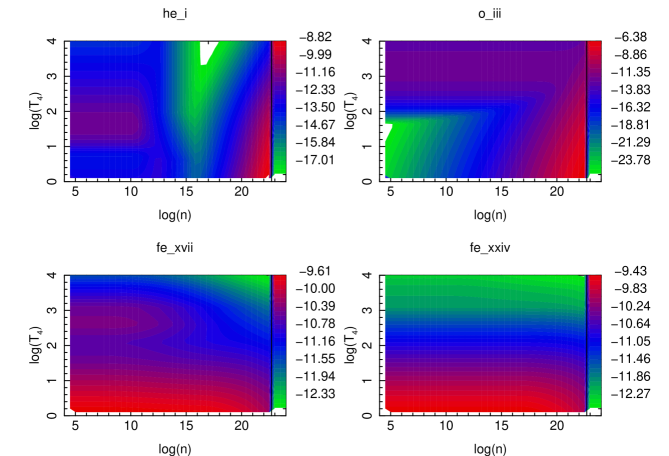
Figure 1: Sample recombination rates vs temperature and density. $T_{4}$ is the temperature in units of 10⁴K. Color represents total rate coefficient in cm³ s^-1

3.2 Ionization Balance

Figure 2 shows the ionization balance for an optically thin gas vs. ionization parameter at various densities shown as colors ${\rm n}_{e}=10^{4}$, $10^{19}$, $10^{20}$, $10^{21}$, $10^{22}$ cm^-3. The low density ${\rm n}_{e}=10^{4}$ cm^-3 results display the general properties of these models: (i) lower ion stages predominate at lower ionization parameter; (ii) higher Z elements are more resistant to ionization and so their mean charge state is lower for a given ionization parameter than for low-Z elements; (iii) the temperature ranges from the Compton temperature $\geq 10^{7}$K at high ionization parameter to $\sim 10^{4}$ K at low ionization parameter where the gas becomes neutral.

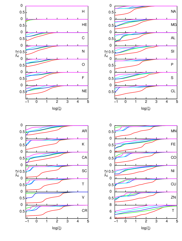
Figure 2: Mean ion charge and log(temperature) vs ionization parameter $\xi=L/nR^{2}$. Colored curves correspond to density: 10⁴ cm^-3 (red), $10^{19}$ cm^-3 (green), $10^{20}$ cm^-3 (blue), $10^{21}$ cm^-3 (turquoise) and $10^{22}$ cm^-3 (purple). Mean charge is displayed as fractions of the element atomic number.

At higher densities ionization potential lowering results in the truncation of the levels down to an energy which is a significant fraction of the low density ionization potential in this case. For example, for H at a density 10²⁰ cm^-3, the ionization potential is lowered by 1.8 eV. This results in lower net recombination into all ions. Figure 2 shows that this has a significant effect throughout parameter space, and that essentially all elements are more highly ionized than when this effect is neglected under the same conditions, owing to the reduced net recombination rate. The temperature is higher owing to free-free heating and reduced collisional cooling.

More detail about the differences between low and high density are shown in Figure 3. This compares the ion fractions for selected elements and temperature for models with low and high density and for high density models with and without some of the high density ingredients. The red curve corresponds to high density with all the ingredients in Section 2 included; the blue curve omits the change in ionization potential; the green curve omits free-free heating. The black curve is the low density curve. This shows that the effect on temperature is to increase the temperature at high density by factors $\geq$ 10 at low ionization parameter. Free-free heating is important at high ionization parameter, and increases the temperature by factors $\geq$2. This result depends on the shape of the illuminating SED, particularly at low energies, and here we have chosen an SED which is weak at low energies. It is clear that most elements are more highly ionized at high densities, due to both the suppression of recombination and also to collisional ionization and reduced recombination due to higher temperatures. The effect of IP lowering, i.e. the difference between the red and blue curves is most apparent for the low-Z elements; IP lowering results in much higher ionization of these elements owing to the fact that the level list for most ions is truncated and recombination is greatly reduced due to the omitted levels. The dependence of this effect on the effective ion charge is apparent in the iron ion fraction distribution: the low charge states show a much greater difference between the red and blue curves while the highest charge states show very little difference.

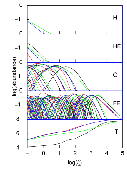
Figure 3: Equilibrium Ion fractions and temperature vs ionization parameter for selected elements, H, He, O, Fe, and temperature. Black curve: density ${\rm n}_{e}=10^{4}$ cm^-3, other curves: density ${\rm n}_{e}=10^{20}$ cm^-3. Red curve: including all density effects including ionization potential lowering on atomic structure; blue curve: same as red but not including ionization potential lowering on atomic structure; green curve: same as blue but not including the effects of free-free heating

3.3 Heating-Cooling

Heating and cooling, and therefore the equilibrium temperature, are affected by density. At low density, electron impact collisions remove energy from the electron thermal bath and thus produce cooling. The rates per unit volume scale with density ${\rm n}_{e}$ as ${\rm n}_{e}^{2}$. Electron impact cooling produces a characteristic local maximum in the cooling function vs. temperature, at temperatures $\sim 10^{5}$ – $10^{6}$K, due to the presence of atomic transitions with energies $\sim 100$ – 1000 eV. This bump is stronger when the gas is at lower ionization, i.e. when photoionization is weak. Heating is due to photoionization, which produces fast photoelectrons which heat as they slow down by scattering with thermal electrons, and also Comptonization which heats due to recoil. Heating rates per unit volume therefore scale as $F{\rm n}_{e}$ where $F$ is the net flux. When both heating and cooling rates are divided by density ${\rm n}_{e}^{2}$, to give the rates per particle, the heating rate is proportional to the ionization parameter $\xi=4\pi F/{\rm n}_{e}$. Figure 4 displays this behavior. The upper left panel shows the net heating and cooling rates $H,\Lambda$ per particle vs temperature for various ionization parameters for the photoionization conditions corresponding to the lowest density shown in Figure 2, i.e. density ${\rm n}_{e}=10^{4}$ cm^-3. Cooling is black, heating is red. Green dots show the equilibrium temperatures. The bump in the cooling curve above $10^{5}$K is apparent, and also the fact that the bump weakens at high $\xi$. The cooling curves have a net increase with temperature, with the exception of the region near the bump, owing to processes which are smoothly varying with temperature including bremsstrahlung and radiative recombination. Higher temperatures result in reduced recombination and increased collisional ionization and therefore net higher ionization of the gas. This results in reduced photoelectric heating at higher temperature, and this is apparent in the red curves. At higher ionization parameter Compton heating and cooling dominate and the curves converge over much of the parameter space. At temperatures $\geq 10^{8}$K, which is not apparent in this Figure, the Compton cooling increases $\propto T$. Other panels in Figure 4 show the behavior of heating and cooling at low density for gas which is held at constant pressure. If so, the relevant ionization parameter is $\Xi=F/(cP)$ (Krolik et al., 1981) where $P$ is the gas pressure. The upper right panel shows the heating and cooling per particle vs. T for various values of $\Xi$. The bottom panels show heating and cooling values in the ($\Xi$-T) plane. On the lower left the values are shown as colors, where the color value corresponds to ${\rm log}(H/{\rm n}_{e}^{2}-\Lambda/{\rm n}_{e}^{2})+20$ for $(H/{\rm n}_{e}^{2}-\Lambda/{\rm n}_{e}^{2})\geq 0$ and $-{\rm log}(\Lambda/{\rm n}_{e}^{2}-H/{\rm n}_{e}^{2})+20$ for $(H/{\rm n}_{e}^{2}-\Lambda/{\rm n}_{e}^{2})\leq 0$. The black curve shows the equilibrium temperature, which has a characteristic ‘S-shape’ indicative of thermal instability. The lower right panel shows contours of constant heating and cooling separately in the ($\Xi$-T) plane. Dashed curves depict heating, solid cooling.

As indicated in Figure 2, at the highest densities three body recombination dominates over other recombination processes. Three body recombination produces net heating since the third electron carries away the energy liberated in the process. This is apparent in Figure 5, which shows heating and cooling at density ${\rm n}_{e}=10^{20}$ cm^-3. Comparison with Figure 4 shows that there is significant heating throughout the parameter space, but greater at higher ionization parameter. Free-free heating also contributes. The resulting equilibrium temperature is greater than at low density by approximately a factor of 10. Another feature of the equilibrium temperature distribution at this density is the disappearance of the thermal instability; the strong temperature-dependent cooling seen at low density is absent. Accompanying this is the fact that the contours of constant heating and cooling are nearly congruent, in contrast to the low density behavior. This is a manifestation of the fact that in local thermodynamic equilibrium (LTE), the heating and cooling balance each other identically at all temperatures, and there is no preferred equilibrium temperature. At the density shown here, LTE is attained for the level populations and rates affecting many of the ions in the gas. This was illustrated in Kallman and Bautista (2001), Figure 10.

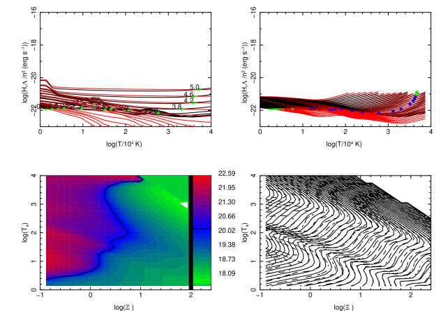
Figure 4: Heating and cooling rates vs. ionization parameter and temperature at density ${\rm n}_{e}=10^{4}$ cm^-3. Upper two panels show heating and cooling. Different curves correspond to different ionization parameter, red=heating, blue=cooling. Green dots correspond to equilibrium values. Upper left panel is for gas which is held at constant density, upper right panel is for gas held at constant pressure. The bottom panels show heating and cooling values in the ($\Xi$-T) plane. On the lower left the values are shown as colors, where the color value corresponds to ${\rm log}(H/{\rm n}_{e}^{2}-\Lambda/{\rm n}_{e}^{2})+20$ for $(H/{\rm n}_{e}^{2}-\Lambda/{\rm n}_{e}^{2})\geq 0$ and $-{\rm log}(\Lambda/{\rm n}_{e}^{2}-H/{\rm n}_{e}^{2})+20$ for $(H/{\rm n}_{e}^{2}-\Lambda/{\rm n}_{e}^{2})\leq 0$. The black curve shows the equilibrium temperature, which has a characteristic ‘S-shape’ indicative of thermal instability. The lower right panel shows contours of constant heating and cooling separately in the ($\Xi$-T) plane. Dashed curves are heating, solid are cooling.

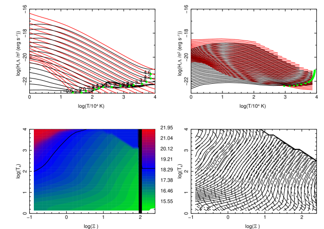
Figure 5: Heating and cooling rates vs. ionization parameter and temperature at density ${\rm n}_{e}=10^{20}$ cm^-3. Upper two panels show heating and cooling. Different curves correspond to different ionization parameter, red=heating, blue=cooling. Green dots correspond to equilibrium values. Upper left panel is for gas which is held at constant density, upper right panel is for gas held at constant pressure. The bottom panels show heating and cooling values in the ($\Xi$-T) plane. On the lower left the values are shown as colors, where the color value corresponds to ${\rm log}(H/{\rm n}_{e}^{2}-\Lambda/{\rm n}_{e}^{2})+20$ for $(H/{\rm n}_{e}^{2}-\Lambda/{\rm n}_{e}^{2})\geq 0$ and $-{\rm log}(\Lambda/{\rm n}_{e}^{2}-H/{\rm n}_{e}^{2})+20$ for $(H/{\rm n}_{e}^{2}-\Lambda/{\rm n}_{e}^{2})\leq 0$. The black curve shows the equilibrium temperature, which has a characteristic ‘S-shape’ indicative of thermal instability. The lower right panel shows contours of constant heating and cooling separately in the ($\Xi$-T) plane. Dashed curves are heating, solid are cooling.

3.4 Line Emissivities

Line emissivities are affected by density in different ways according to the dominant process for the line emission. Lines emitted by recombination or electron impact collisions depend on density according to ${\rm n}_{e}^{2}$. Lines emitted by resonance scattering or fluorescence are proportional to gas density and the radiation flux, which is equivalent to density ${\rm n}_{e}^{2}\xi$. In the previous subsection we have shown that the high density model with ${\rm n}_{e}=10^{20}$ cm^-3 produces higher ionization and higher temperature than the ${\rm n}_{e}=10^{4}$ cm^-3 model. The generally higher ionization balance shifts the line emissivity in ionization parameter space. Figure 6 shows the emissivities in units erg cm³ s^-1, i.e. emissivity with the density ${\rm n}_{e}^{2}$ dependence divided. Comparison of the panels of Figure 6 shows that the density ${\rm n}_{e}^{2}$ scaling works in an approximate sense, the envelope of most of the emissivities is similar between the two densities. The emissivities per ion are very similar between the two models, though the curves for each ion are shifted towards lower $\xi$ in the high density models. This suggests that, when these rates are used to calculate the flux from a physical model for a X-ray illuminated slab of gas at density ${\rm n}_{e}=10^{20}$ cm^-3, the total line flux escaping the slab will be similar to a low density model, though shifted in energy owing to the higher degree of ionization. In this paper, we will not present physical model slabs, since these depend on solutions to the radiative transfer equation, and that is beyond the scope of this paper. We will present such models in a future publication.

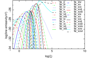
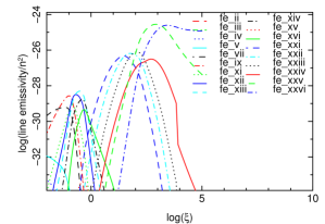
Figure 6: Line emissivities vs. ionization parameter log($\xi$) at density ${\rm n}_{e}=10^{4}$ (left) and ${\rm n}_{e}=10^{20}$ cm^-3 (right).

3.5 Opacity and Emissivity

The opacity of gas at high density differs from that at low density due to the free-free opacity. This is apparent in comparison of Figures 7 and 8. The left hand panels show the opacity vs. energy at various ionization parameters. The opacity is small at high ionization parameter, so opacity is dominated by Thomson scattering. Photoelectric opacity gains in importance at lower ionization parameter, with significant energy dependence. At the highest ionization parameters edges due to highly ionized Fe and Ni are apparent. At lower ionization parameter, log($\xi$)$\sim$ 0 – 2, there is strong opacity between $\sim$0.5 – 2 keV from intermediate-Z elements. At low ionization parameter bound-free opacity from H and He and from valence shells of low ionization metals dominate. At high density opacity from these ions are augmented by free-free opacity which has power law behavior in energy.

Emissivity behaves in an analogous way, progressing from predominantly free-free at high ionization parameter to radiative recombination continua (RRCs) (Liedahl et al., 1990) at lower ionization parameter. The low- and high density models differ at low energies, where the low density models shows a strong increase in total emissivity at low ionization parameters. The high density models do not, owing to the fact that the ionization balance is changing less with ionization parameter.

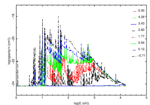
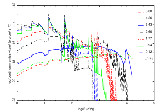
Figure 7: Opacity (left) and continuum emissivity (right) for a low density ${\rm n}_{e}=10^{4}$ cm^-3 model for various values of ionization parameter shown log($\xi$) in the legend. Thomson opacity is not included.

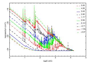
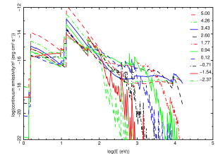
Figure 8: Opacity (left) and continuum emissivity (right) for a hith density ${\rm n}_{e}=10^{20}$ cm^-3 model for various values of ionization parameter shown in the legend. Thomson opacity is not included.

3.6 Level Populations

At high density many of the levels of ground terms and configurations become populated by collisions, i.e. the collisional rates linking the levels become faster than the radiative decays. This is an extension of the familiar process leading to population of metastable levels in nebulae. Observations in many cases constrain these populations via the line emission or absorption indicating population of the upper or lower levels. An illustration is the B-like ion Fe XXII, in which the $2s^{2}2p$ ground term is split into the $j=1/2$ ground level and $j=3/2$ excited level. The critical density leading to population of the excited levels is $\sim 10^{14}$ cm^-3 (Mauche et al., 2004). Above this density the line $2s^{2}2p_{3/2}-2s^{2}3d_{5/2}$ at 11.92 $\AA$ can appear in absorption, in addition to the ground state line $2s^{2}2p_{1/2}-2s^{2}3d_{3/2}$ at 11.77 $\AA$. The 11.92 $\AA$ line has been detected in astrophysical systems including the black hole transient GROJ1655-40 (Miller et al., 2006), and this is indicative of reprocessing in a high density medium. It has also been used by King et al. (2012) to constrain absorber density in in the Seyfert-1 Galaxy NGC 4051.

Figure 9 shows the spectrum predicted by xstar in the region containing the Fe XXII lines, together with the $Chandra$ High Energy Transmission Grating (HETG) spectrum of GROJ1655-40 (Miller et al., 2006). The three panels correspond to densities ${\rm n}_{e}=10^{4}$ cm^-3, $10^{16}$ cm^-3, $10^{20}$ cm^-3. The data clearly shows the presence of both the 11.77 and 11.92 $\AA$ lines. The panels show that the ${\rm n}_{e}=10^{4}$ cm^-3 model fits the 11.77 $\AA$ line but fails to fit the 11.92 $\AA$ line. The ${\rm n}_{e}=10^{16}$ cm^-3 model fits both lines qualitatively. The ${\rm n}_{e}=10^{20}$ cm^-3 model shows the presence of many other lines arising from excited levels which require this density for excitation. Notable among them is the line at 11.748 $\AA$ which arises from the $2s2p^{2}(^{3}D_{3/2})$ level. This line is stronger than the 11.97 $\AA$ line at this density. This illustrates that the absence of such lines in the spectrum sets an upper limit on the density in this source.

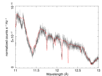
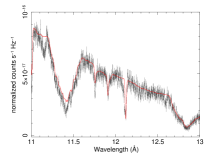
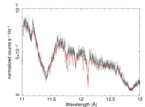
Figure 9: Fits to the $Chandra$ HETG spectrum of GROJ1655-40 as obtained by Miller et al. (2006). Models are at densities ${\rm n}_{e}=10^{4}$ (left), $10^{16}$ (middle), and $10^{20}$ (right) cm^-3. The effect of metastable population on the $2s^{2}3d_{5/2}$ level on the 11.92$\AA$ line is apparent in the middle panel. The effect of the $2s2p^{2}(^{3}D_{3/2})$ level on the 11.748 $\AA$ line is apparent in the right panel.

4 Conclusions

In this paper we have explored the effects of high densities on models for astrophysical gas ionized and heated by photoionization. Our models are valid up to density ${\rm n}_{e}\sim 10^{22}$ cm^-3; we have illustrated our results with models at ${\rm n}_{e}\sim 10^{20}$ cm^-3. We have shown that:

• As density is increased above ${\rm n}_{e}\sim 10^{4}$ cm^-3, the net recombination decreases, due to the suppression of dielectronic recombination, leading to generally higher ionization for comparable conditions.

• This trend is reversed at higher density ${\rm n}_{e}\geq 10^{15}$ cm^-3, due to the onset of three body recombination, leading to generally lower ionization for comparable conditions.

• Lower ionization generally leads to greater photoionization heating, and thus higher temperature.

• Stimulated recombination becomes important at high radiation intensities, and this accompanies high gas densities when the ionization parameter is held fixed. The net effect is similar to the effect of three body recombination.

• Additional heating at high density comes from free-free heating, again due to the greater local radiation intensity.

• When the effective ionization potential is reduced due to Debye screening to the point where many excited levels are in the continuum, the behavior of many ions changes qualitatively. The net recombination rate is again reduced, and line emission and cooling efficiencies are also reduced.

• Many of these processes depend on the effective charge of the ion: higher densities are needed to make three body recombination important for highly charged ions compared with near-neutrals; continuum lowering effects are more important for low charge ions, compared with highly charged ions at a given density.

• Comparison of ionization and thermal balance between low (${\rm n}_{e}=10^{4}$ cm^-3) and high density (${\rm n}_{e}=10^{20}$ cm^-3) photoionization models shows that the latter are hotter by up to a factor of 10, and significantly more highly ionized for a given ionization parameter. Thermal instability at constant pressure does not occur.

• Line emissivities and opacities generally obey simple scaling behavior, but there are important departures which will affect model spectra.

• Densities greater than those considered previously lead to excitation of new metastable levels and accompanying line formation.

The xstar atomic rate coefficients and code calculating ionization balance, atomic level populations, temperature, emissivity and opacity is also used in calculation of the reflection spectra from Compton-thick atmospheres with the xillver code by García & Kallman (2010); García et al. (2011, 2013). These models also allow treatment of angle dependence of the radiation field, both the effect of non-normal incident radiation and also the angle dependence of the reflected radiation. In subsequent papers we will present models at densities appropriate to astrophysical sources which exhibit reflection spectra. These will include all the ingredients of the García et al. (2013) models, and span similar free parameter values, plus include the revisions to atomic rate coefficients described so far.

Appendix A Appendix

It is worthwhile to compare the particular effects of the density, and other recent changes to predictions of xstar to typical variations between the predictions of other models and codes designed for solving similar problems. These have been described in the proceedings of the series of non-LTE workshops, and in the publications by Ralchenko (2016); Hansen et al. (2020). Most of these codes have been applied extensively to terrestrial plasmas, such as laser-produced plasmas. Comparisons with those codes necessarily focusses on elements which are of interest to astrophysics. We have compared xstar results with two of the models described in the compilation of model results by Hansen et al. (2020).

The first comparison is a model for Si produced primarily by photoionization, denoted ’steady state Si’ in that paper. The ionizing spectrum is chosen to be a blackbody with kT=63 eV, with flux specified as either the full blackbody or else diluted by 10x. We compare with the models with density $10^{19}$ cm^-3, which then corresponds to ionization parameter values log($\xi$)=1.3 or 0.3. The resulting ionization balance of these models are shown in figure 10. The ensemble of other code results are shown as grey curves and xstar is shown in red. This shows that our models produce an ionization balance which is slightly less than most other models for the high-$\xi$ model but is very similar to the other models for the low-$\xi$ model.

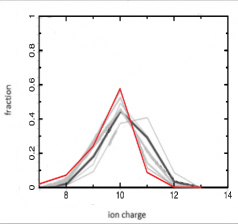
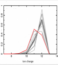
Figure 10: Comparison of charge state distribution between the ensemble of models described in Hansen et al. (2020) for silicon with photoionization (grey curves) and an xstar model for similar conditions (red curve). Right panel: undiluted blackbody illumination; Left panel: diluted blackbody illumination by 10x

The second comparison is a model for Ne produced by collisional ionization, denoted ’steady state Ne’ by Hansen et al. (2020). We compare with the models with density $10^{19}$ cm^-3 and $10^{21}$ cm^-3. The resulting mean charge vs. temperature is shown in figure 11. The ensemble of other code results are shown as grey curves and xstar is shown in red. This shows that our models produce mean ion charge which is less than the average of the other models by 0.2 dex for both densities, though we note the dispersion among the other results is larger than this. We also note that the change in the mean charge between the two densities is also $\sim$0.2 dex, and that this is similar to the behavior of the mean of the models shown in Hansen et al. (2020). The xstar results are derived from the rates from Bryans et al. (2006) at low density, and agree with those results identically at density 10⁴ cm^-3. At higher density the xstar results predict lower mean ion charge than the models cited in the Hansen et al. (2020) compilation by about 0.1 dex on average. One possible reason for this is the treatment of electron impact excitation from metastable levels to doubly excited levels, which then autoionize. This process is included in the low density rates from Bryans et al. (2006) for collisions from the ground state, but xstar likely has fewer such transitions included for metastables states which are populated at density $\geq 10^{19}$ cm^-3.

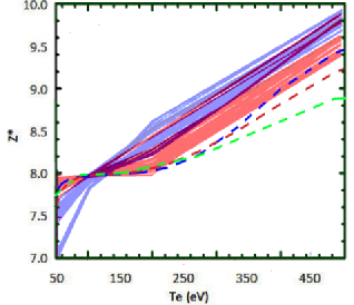
Figure 11: Comparison of mean ion charge vs. temperature between the ensemble of models described in Hansen et al. (2020) for neon with coronal conditions.(solid curves) and xstar models for similar conditions (dashed curves). Colors correspond to density 10¹⁹ cm^-3 (blue) 10²¹ cm^-3 (red). Density 10⁴ cm^-3 (green) is shown for xstar only.

References

- (1)
- Aldrovandi & Pequignot (1973) Aldrovandi, S. M. V., & Pequignot, D. 1973, A&A, 25, 137
- Badnell et al. (1993) Badnell, N. R., Pindzola, M. S., Dickson, W. J., et al. 1993, ApJ, 407, L91
- Badnell (1997) Badnell, N. R. 1997, J. Phys. B, 30, 1
- Badnell et al. (2003) Badnell, N. R., O’Mullane, M. G., Summers, H. P., et al. 2003, A&A, 406, 1151
- Badnell (2011) Badnell, N. R. 2011, Computer Physics Communications, 182, 1528
- Balbus & Hawley (1991) Balbus, S. A., & Hawley, J. F. 1991, ApJ, 376, 214
- Bautista et al. (2000) Bautista, M., et al 2000, ApJ 544, 581; Bautista et al. 1998, ApJ 509, 848
- Bautista and Kallman (2001) Bautista, M., and Kallman, T., 2001 Ap. J. Supp. 134, 139
- Bautista et al. (1998) Bautista, M. A., Kallman, T. R., Angelini, L., Liedahl, D. A., & Smits, D. P. 1998, ApJ, 509, 848
- Berrington et al. (1995) Berrington, K. A., Eissner, W. B., & Norrington, P. H. 1995, Computer Physics Communications, 92, 290
- Bryans et al. (2006) Bryans, P., Badnell, N. R., Gorczyca, T. W., et al. 2006, ApJS, 167, 343. doi:10.1086/507629
- Cackett et al. (2010) Cackett, E. M., Miller, J. M., Ballantyne, D. R., et al. 2010, ApJ, 720, 205
- Chamberlain (1961) Chamberlain, J. W. 1961, Ap. J., 133, 675
- Chaudhary et al. (2012) Chaudhary, P., Brusa, M., Hasinger, G., et al. 2012, A&A, 537, A6
- Cowan (1981) Cowan, R. D. 1981, Los Alamos Series in Basic and Applied Sciences
- Dauser et al. (2014) Dauser, T., Garcia, J., Parker, M. L., et al. 2014, MNRAS, 444, L100
- Davis and Blaha (1982) Davis, J., and Blaha, M.. 1982 J. Quant. Spectr. Rad. Transfer, 307, 313.
- Deprince et al. (2020a) Deprince, J., Bautista, M. A., Fritzsche, S., et al. 2020a, A&A, 635, A70
- Deprince et al. (2020b) Deprince, J., Bautista, M. A., Fritzsche, S., et al. 2020b, A&A, 643, A57
- Deprince et al. (2019b) Deprince, J., Bautista, M. A., Fritzsche, S., et al. 2019b, A&A, 626, A83
- Deprince et al. (2019a) Deprince, J., Bautista, M. A., Fritzsche, S., et al. 2019a, A&A, 624, A74
- Devereux & Heaton (2013) Devereux, N., & Heaton, E. 2013, ApJ, 773, 97
- Dufresne, et al. (2020) Dufresne, R. P., G Del Zanna, G., Badnell, N. R., arXiv:2007.00465, 2020
- Falocco et al. (2013) Falocco, S., Carrera, F. J., Corral, A., et al. 2013, arXiv:1304.7690
- Gabel et al. (2003) Gabel, J., et al. 2003, Ap J 595 120
- García et al. (2019) García, J. A., Kara, E., Walton, D., et al. 2019, ApJ, 871, 88
- García et al. (2018) García, J. A., Steiner, J. F., Grinberg, V., et al. 2018, ApJ, 864, 25
- García et al. (2016) García, J. A., Fabian, A. C., Kallman, T. R., et al. 2016, MNRAS, 462, 751
- García et al. (2014) García, J., Dauser, T., Lohfink, A., et al. 2014, ApJ, 782, 76
- García et al. (2013) García, J., Dauser, T., Reynolds, C. S., et al. 2013, ApJ, 768, 146
- García et al. (2011) García, J., Kallman, T. R., & Mushotzky, R. F. 2011, ApJ, 731, 131
- García & Kallman (2010) García, J., & Kallman, T. R. 2010, ApJ, 718, 695
- García et al. (2018b) García, J. A., Kallman, T. R., Bautista, M., et al. 2018, Workshop on Astrophysical Opacities, 282
- Gottwald et al. (1995) Gottwald, M., Parmar, A. N., Reynolds, A. P., et al. 1995, A&AS, 109, 9
- Grant et al. (1980) Grant, I. P., McKenzie, B. J., Norrington, P. H., et al. 1980, Computer Physics Communications, 21, 207
- Hahn (1997) Hahn, Y. 1997, Physics Letters A, 231, 82
- Hansen et al. (2020) Hansen, S. B., Chung, H.-K., Fontes, C. J., et al. 2020, High Energy Density Physics, 35, 100693. doi:10.1016/j.hedp.2019.06.001
- Hummer & Mihalas (1988) Hummer, D. G. & Mihalas, D. 1988, ApJ, 331, 794. doi:10.1086/166600
- Inglis & Teller (1939) Inglis, D. R., & Teller, E. 1939, ApJ, 90, 439
- Jiang et al. (2019) Jiang, J., Fabian, A. C., Wang, J., et al. 2019, MNRAS, 484, 1972
- Jiang et al. (2019) Jiang, J., Fabian, A. C., Dauser, T., et al. 2019, MNRAS, 489, 3436
- Jiang et al. (2018) Jiang, J., Parker, M. L., Fabian, A. C., et al. 2018, MNRAS, 477, 3711
- Kallman and Bautista (2001) Kallman, T. R. and Bautista, M., 2001 Ap. J. Supp 133,221
- Kallman & Palmeri (2007) Kallman, T. R., & Palmeri, P. 2007, Reviews of Modern Physics, 79, 79
- Kallman et al. (2004) Kallman, T. R., Palmeri, P., Bautista, M. A., Mendoza, C., & Krolik, J. H. 2004, Ap. J. Supp., 155, 675
- Kaspi et al. (2001) Kaspi, S., et al. 2001, ApJ, 554, 216
- Kaspi et al. (2002) Kaspi, S., et al., 2002, Ap. J., 574, 643
- King et al. (2012) King, A. L., Miller, J. M., & Raymond, J. 2012, ApJ, 746, 2
- Krstic and Hahn (1996) Krstic, P., and Hahn, Y. 1996, J. Quant. Spec. Radiat. Transf., 55, 499
- Krolik et al. (1981) Krolik, J. H., McKee, C. F., & Tarter, C. B. 1981, ApJ, 249, 422
- Krolik & Kallman (1987) Krolik, J. H., & Kallman, T. R. 1987, ApJ, 320, L5
- Kwan & Krolik (1981) Kwan, J., & Krolik, J. H. 1981, ApJ, 250, 478
- Landi et al. (2013) Landi, E., Young, P. R., Dere, K. P., Del Zanna, G., & Mason, H. E. 2013, ApJ, 763, 86
- Lee et al. (2001) Lee, J. C., Ogle, P. M., Canizares, C. R., Marshall, H. L., Schulz, N. S., Morales, R., Fabian, a. C., Iwasawa, K. 2001, ApJ, 554, L13
- Lee, et al. (2008) Lee, J., Young, A., and Kallman, T., 2008, Ap. J. submitted
- Liedahl et al. (1990) Liedahl, D. A., Kahn, S. M., Osterheld, A. L., et al. 1990, ApJ, 350, L37
- Ludlam et al. (2020) Ludlam, R. M., Cackett, E. M., García, J. A., et al. 2020, ApJ, 895, 45
- Mallick et al. (2018) Mallick, L., Alston, W. N., Parker, M. L., et al. 2018, MNRAS, 479, 615
- Matt et al. (1993) Matt, G., Fabian, A. C., & Ross, R. R. 1993, MNRAS, 262, 179
- Mauche et al. (2004) Mauche, C. W., Liedahl, D. A., & Fournier, K. B. 2004, IAU Colloq. 190: Magnetic Cataclysmic Variables, 124
- McClintock & Remillard (2006) McClintock, J. E., & Remillard, R. A. 2006, Compact stellar X-ray sources, 157
- Mendoza et al. (2018) Mendoza, C., Bautista, M. A., Palmeri, P., et al. 2018, A&A, 616, A62
- Mendoza et al. (2017) Mendoza, C., Bautista, M. A., Palmeri, P., et al. 2017, A&A, 604, A63
- Miller et al. (2006) Miller, J. M., Raymond, J., Fabian, A., et al. 2006, Nature, 441, 953
- Miller (2007) Miller, J. M. 2007, ARA&A, 45, 441
- Murray et al. (2005) Murray, N., Quataert, E., and Thompson, T., 2004 618, 569
- Nandra et al. (1997) Nandra, K., George, I. M., Mushotzky, R. F., Turner, T. J., & Yaqoob, T. 1997, ApJ, 488, L91
- Nandra et al. (2007) Nandra, K., O’Neill, P. M., George, I. M., & Reeves, J. N. 2007, MNRAS, 382, 194
- Nikolić et al. (2013) Nikolić, D., Gorczyca, T. W., Korista, K. T., Ferland, G. J., & Badnell, N. R. 2013, ApJ, 768, 82
- Noble et al. (2010) Noble, S. C., Krolik, J. H., & Hawley, J. F. 2010, ApJ, 711, 959
- Ogorzalek et al. (2020) Ogorzalek, A., et al., 2020 in preparation.
- Palmeri et al. (2016) Palmeri, P., Quinet, P., Mendoza, C., et al. 2016, A&A, 589, A137
- Palmeri et al. (2012) Palmeri, P., Quinet, P., Mendoza, C., et al. 2012, A&A, 543, A44
- Palmeri et al. (2003) Palmeri, P., Mendoza, C., Kallman, T. R., Bautista, M. A., & Meléndez, M. 2003, A&A, 410, 359
- Parker et al. (2018) Parker, M. L., Miller, J. M., & Fabian, A. C. 2018, MNRAS, 474, 1538
- Ralchenko (2016) Ralchenko, Y. 2016 “Modern Methods in Collisional-Radiative Modeling of Plasmas” Springer: New York
- Rees et al. (1989) Rees, M. J., Netzer, H., & Ferland, G. J. 1989, ApJ, 347, 640
- Reis & Miller (2013) Reis, R. C., & Miller, J. M. 2013, ApJ, 769, L7
- Reynolds & Fabian (1997) Reynolds, C. S., & Fabian, A. C. 1997, MNRAS, 290, L1
- Reynolds & Nowak (2003) Reynolds, C. S., & Nowak, M. A. 2003, Phys. Rep., 377, 389
- Reynolds & Fabian (2008) Reynolds, C. S., & Fabian, A. C. 2008, ApJ, 675, 1048
- Reynolds et al. (2012) Reynolds, C. S., Brenneman, L. W., Lohfink, A. M., et al. 2012, ApJ, 755, 88
- Reynolds (2013) Reynolds, C. S. 2013, arXiv:1302.3260
- Ross & Fabian (2005) Ross, R. R., & Fabian, A. C. 2005, MNRAS, 358, 211
- Ross & Fabian (2007) Ross, R. R., & Fabian, A. C. 2007, MNRAS, 381, 1697
- Sahoo & Ho (2006) Sahoo, S., & Ho, Y. K. 2006, Physics of Plasmas, 13, 063301
- Sazonov & Sunyaev (2001) Sazonov, S. Y., & Sunyaev, R. A. 2001, Astronomy Letters, 27, 481
- Schnittman et al. (2013) Schnittman, J. D., Krolik, J. H., & Noble, S. C. 2013, ApJ, 769, 156
- Shakura & Sunyaev (1973) Shakura, N. I., & Sunyaev, R. A. 1973, A&A, 24, 337
- Steiner et al. (2012) Steiner, J. F., Reis, R. C., Fabian, A. C., et al. 2012, MNRAS, 427, 2552
- Summers (1972) Summers, H. P. 1972, MNRAS, 158, 255
- Tomsick et al. (2018) Tomsick, J. A., Parker, M. L., García, J. A., et al. 2018, ApJ, 855, 3
- Uttley et al. (2014) Uttley, P., Cackett, E. M., Fabian, A. C., et al. 2014, A&A Rev., 22, 72
- Wang-Ji et al. (2018) Wang-Ji, J., García, J. A., Steiner, J. F., et al. 2018, ApJ, 855, 61
- Weisheit & Murillo (2006) Weisheit, J. & Murillo, M. 2006, Springer Handbook of Atomic, 1303. doi:10.1007/978-0-387-26308-3_86