Entanglement Spectrum Crossings Reveal non-Hermitian Dynamical Topology

Abstract

The development of non-Hermitian topological band theory has led to observations of novel topological phenomena in effectively classical, driven and dissipative systems. However, for open quantum many-body systems, the absence of a ground state presents a challenge to define robust signatures of non-Hermitian topology. We show that such a signature is provided by crossings in the time evolution of the entanglement spectrum. These crossings occur in quenches from the trivial to the topological phase of a driven-dissipative Kitaev chain that is described by a Markovian quantum master equation in Lindblad form. At the topological transition, which can be crossed either by changing parameters of the Hamiltonian of the system or by increasing the strength of dissipation, the time scale at which the first entanglement spectrum crossing occurs diverges with a dynamical critical exponent of $\epsilon=1/2$. We corroborate these numerical findings with an exact analytical solution of the quench dynamics for a spectrally flat postquench Liouvillian. This exact solution suggests an interpretation of the topological quench dynamics as a fermion parity pump. Our work thus reveals signatures of non-Hermitian topology which are unique to quantum many-body systems and cannot be emulated in classical simulators of non-Hermitian wave physics.

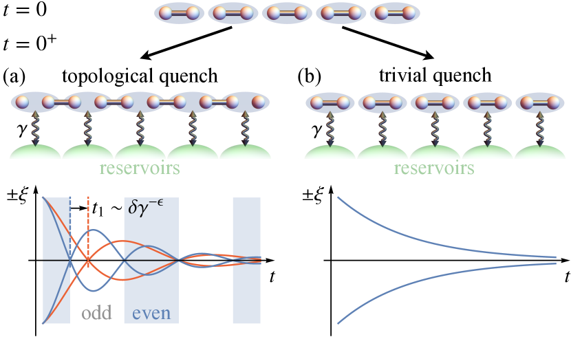
Figure 1: Quench dynamics of a driven-dissipative Kitaev chain. At $t=0$, the system is prepared in the topologically trivial ground state of the Kitaev chain, where Majorana fermions (spheres) pair locally (gray bonds) at each site of the chain (blue ellipses). Then, at $t=0^{+}$, the system is driven out of its initial state by an abrupt change of the chemical potential. Simultaneously, the chain is connected to Markovian reservoirs, which induce dissipation at a rate $\gamma$. (a) For quenches to the topological phase of the postquench Liouvillian, the entanglement spectrum exhibits oscillatory decay with repeated zero crossings (only a single pair of entanglement eigenvalues $\pm\xi$ is shown as blue lines in the figure). At each zero crossing, the fermion parity of the entanglement ground state switches between even and odd. Red lines show the evolution of $\pm\xi$ for a quench closer to the topological phase boundary at $\gamma_{\mathrm{c}}$. For $\delta\gamma=\left\lvert\gamma-\gamma_{\mathrm{c}}\right\rvert\to 0$, the time $t_{1}$ at which the first crossing occurs diverges as $t_{1}\sim\delta\gamma^{-\epsilon}$ with a universal critical exponent $\epsilon=1/2$. (b) For quenches to a trivial phase, the entanglement eigenvalues $\pm\xi$ decay without crossing zero.

I Introduction

Non-Hermitian topological band theory Esaki et al. (2011); Malzard et al. (2015); Leykam et al. (2017); Shen et al. (2018); Gong et al. (2018); Yao and Wang (2018); Kunst et al. (2018); Kawabata et al. (2019); Zhou and Lee (2019); Liu et al. (2019); Yokomizo and Murakami (2019); Borgnia et al. (2020); Ashida et al. (2020) allows to derive a topological classification of the complex spectra of quadratic Liouvillians Lieu et al. (2020); Dangel et al. (2018); Lieu (2019); Song et al. (2019); Minganti et al. (2019); Liu et al. (2020); Okuma and Sato (2020), which describe the dynamics of noninteracting, driven and open quantum many-body systems. For complex spectra, the very notions of a ground state, as well as of filled and empty bands, are ill-defined. In the topological band theory for isolated and noninteracting fermionic systems, however, these concepts are central to predict robust topological features, such as the quantized response of a system in its ground state Hasan and Kane (2010); Qi and Zhang (2011); Chiu et al. (2016). Moreover, the existence of a ground state allows to generalize topological phases to interacting many-body systems Chiu et al. (2016). These observations raise the question that motivates our work: Which robust signatures of non-Hermitian topology survive in driven and open quantum many-body systems? Here we propose that the time evolution of the entanglement spectrum can provide such a signature.

The entanglement spectrum is a powerful tool to detect the presence of topological order in the pure ground state $\lvert\psi_{0}\rangle$ of the Hamiltonian $H_{0}$ of an isolated Hermitian system Li and Haldane (2008); Pollmann et al. (2010); Fidkowski (2010); Thomale et al. (2010); Cirac et al. (2011); Chandran et al. (2011); Qi et al. (2012); Schuch et al. (2013); Regnault (2017). For a subsystem $A$ and its complement $A^{\mathrm{c}}$, the many-body entanglement spectrum is defined as the spectrum of the reduced density matrix $\rho_{A}={\mathop{\mathrm{tr}}}_{A^{\mathrm{c}}}(\rho_{0})$, where $\rho_{0}=\lvert\psi_{0}\rangle\langle\psi_{0}\rvert$ is the density matrix that is associated with the pure state $\lvert\psi_{0}\rangle$. The bulk-edge correspondence of the entanglement spectrum Chandran et al. (2011); Qi et al. (2012) establishes a one-to-one correspondence between the low-energy edge states of the physical Hamiltonian at an open boundary of subsystem $A$, and the entanglement eigenstates of $\rho_{A}$ that have the highest entanglement eigenvalues, i.e., that are most entangled with the rest of the system. This correspondence holds both for noninteracting and interacting systems, and has even been applied to systems which are driven out of equilibrium: After a sudden quench from $H_{0}$ to $H$, the time-evolved state $\lvert\psi(t)\rangle=\mathrm{e}^{-\mathrm{i}Ht}\lvert\psi_{0}\rangle$ is the ground state of the time-dependent parent Hamiltonian $H_{\mathrm{p}}(t)=\mathrm{e}^{-\mathrm{i}Ht}H_{0}\mathrm{e}^{\mathrm{i}Ht}$, and the entanglement spectrum of $\lvert\psi(t)\rangle$ reflects the topology of $H_{\mathrm{p}}(t)$ Gong and Ueda (2018); Chang (2018); Lu and Yu (2019); Pastori et al. (2020).

Despite the strikingly universal applicability of the entanglement spectrum as a diagnostic for topological order, it is unclear whether the non-Hermitian topology of the complex spectrum of a Liouvillian $\hat{\mathcal{L}}$ leaves signatures in the entanglement spectrum of an associated quantum state. For example, the time-evolved density matrix $\rho(t)=\mathrm{e}^{\hat{\mathcal{L}}t}\rho_{0}$ is, in general, a mixed state. Therefore, it cannot be interpreted as the ground state of any putative non-Hermitian parent Hamiltonian $H(t)$. Intriguingly, establishing the connection between the entanglement spectrum of $\rho(t)$ and the topology of $\hat{\mathcal{L}}$ could open up the possibility to characterize the non-Hermitian topology of both noninteracting and interacting open quantum many-body systems.

In this paper, we show that non-Hermitian dynamical topology of driven and open quantum many-body systems is revealed by crossings in the time evolution of the entanglement spectrum after a quench. We consider a Kitaev chain, which is subject to Markovian gain and dissipation Klett et al. (2017); Menke and Hirschmann (2017); Li et al. (2018); Kawabata et al. (2018); van Caspel et al. (2019) as illustrated in Fig. 1. The topology of the corresponding Liouvillian is characterized by a non-Hermitian winding number $W$ Esaki et al. (2011); Kawabata et al. (2019). A quench from a trivial to a topological phase leads to stable crossings in the entanglement spectrum of the time-evolved density matrix $\rho(t)$ as shown in Fig. 1(a). Instead, as illustrated in Fig. 1(b), the dynamics after a quench to a trivial phase does not feature such crossings. We show that topological entanglement spectrum crossings can be traced back to the reversal of the fermion parity in individual entanglement eigenstates. Thus, our work establishes that entanglement spectrum crossings and the concomitant pumping of fermion parity are robust signatures of non-Hermitian dynamical topology of the Liouvillian.

Surprisingly, we obtain these results for systems which heat up to a featureless infinite-temperature state at late times. By contrast, much previous work focused on inducing nontrivial topological features in the steady state $\rho_{\mathrm{ss}}=\lim_{t\to\infty}\rho(t)$, which can be achieved by properly designing purely dissipative dynamics Diehl et al. (2011); Bardyn et al. (2013); Goldstein (2018); Shavit and Goldstein (2020); Tonielli et al. (2020). Adopting this point of view, one is led to the conclusion that the systems we study are trivial. Instead, the perspective taken in this work, which is inspired by non-Hermitian band theory Esaki et al. (2011); Malzard et al. (2015); Leykam et al. (2017); Shen et al. (2018); Gong et al. (2018); Yao and Wang (2018); Kunst et al. (2018); Kawabata et al. (2019); Zhou and Lee (2019); Liu et al. (2019); Yokomizo and Murakami (2019); Borgnia et al. (2020); Ashida et al. (2020), focuses on the topological properties of the Liouvillian. As explained above, these properties are revealed in the dynamics, i.e., in the approach to the steady state. The time evolution of the entanglement spectrum reveals a sharp dynamical topological phase transition with associated dynamical criticality, reflected in a divergence of the time scale on which entanglement spectrum crossings occur as illustrated in Fig. 1(a). These features highlight the stark contrast between the two complementary approaches to the topology of driven and open quantum many-body systems: the one based on $\rho_{\mathrm{ss}}$ Diehl et al. (2011); Bardyn et al. (2013); Goldstein (2018); Shavit and Goldstein (2020); Tonielli et al. (2020), and the one that we propose, which is based on the entanglement spectrum.

We finally emphasize that the characterization of topology in terms of entanglement spectrum crossings is unique to quantum many-body systems and cannot be emulated by photonic Zeuner et al. (2015); Poli et al. (2015); Weimann et al. (2017); Xiao et al. (2017); Zhao et al. (2018); Zhou et al. (2018); Parto et al. (2018); Xiao et al. (2020); Pickup et al. (2020); Wang et al. (2020); Fedorova et al. (2020) or mechanical Zhu et al. (2018) simulators of non-Hermitian wave physics. Moreover, by using the entanglement spectrum as a tool to diagnose non-Hermitian topology, our work paves the way to characterize non-Hermitian dynamical topology also of interacting open quantum many-body systems.

This paper is organized as follows: We present our main results in Sec. II. The model and formalism on which our study is based are introduced in Sec. III, and we summarize the non-Hermitian topological band theory of the driven-dissipative Kitaev chain in Sec. IV. The relationship between entanglement spectrum crossings and non-Hermitian topology of the Liouvillian depends on whether the jump operators, which describe the coupling of the system to Markovian reservoirs, are Hermitian or non-Hermitian. Section V is devoted to systems with Hermitian jump operators. In particular, we discuss the time evolution of entanglement spectra, the connection between entanglement spectrum crossings and parity pumping, and dynamical criticality. We consider systems non-Hermitian jump operators in Sec. VI. Our conclusions are presented in Sec. VII, together with an outlook on future perspectives. Technical details are deferred to Appendices A–G.

II Summary of main results

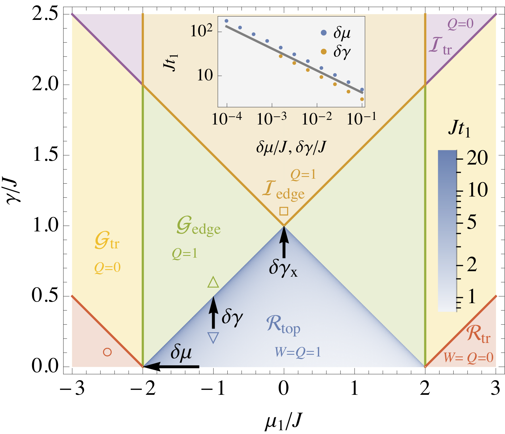
Figure 2: Dynamical topological phase diagram and dynamical criticality of entanglement spectrum crossings. The non-Hermitian winding number $W$ (for phases with real line gaps) and the global Berry phase $Q$ distinguish six dynamical phases: the real-line gapped phases with nontrivial ($\mathcal{R}_{\mathrm{top}}$, with $W=Q=1$) and trivial ($\mathcal{R}_{\mathrm{tr}}$, with $W=Q=0$) topology, the imaginary-line gapped phases with ($\mathcal{I}_{\mathrm{edge}}$, with $Q=1$) and without ($\mathcal{I}_{\mathrm{tr}}$, with $Q=0$) edge states, and the gapless phases with ($\mathcal{G}_{\mathrm{edge}}$, with $Q=1$) and without ($\mathcal{G}_{\mathrm{tr}}$, with $Q=0$) edge states. Entanglement spectrum crossings occur for quenches from the trivial phase of the isolated Kitaev chain to $\mathcal{R}_{\mathrm{top}}$. The logarithmic color scale in $\mathcal{R}_{\mathrm{top}}$ encodes the time $t_{1}$ of the first entanglement spectrum zero crossing for a quench with $\mu_{0}=-3J$ and in a system of size $N=100$. Inset: $t_{1}$ diverges at the boundary of $\mathcal{R}_{\mathrm{top}}$ with a critical exponent of $\epsilon=1/2$. The data shown corresponds to approaching the phase boundary along the black arrows labeled by $\delta\mu$ and $\delta\gamma$ in the main panel: $\mu_{1}=-2J+\delta\mu$, $\gamma=0$ for the blue dots, and $\mu_{1}=-J$, $\gamma=0.5J-\delta\gamma$ for the orange dots. In the former case, longer evolution times can be reached due to the absence of decay. The system size is $N=1000$. For comparison, the gray solid line shows a square-root singularity.

We consider the following model and quench protocol: At time $t=0$, a Kitaev chain is prepared in its ground state $\lvert\psi_{0}\rangle$ with a chemical potential $\mu_{0}$, which is then changed abruptly to $\mu_{1}$ at $t=0^{+}$. Simultaneously, the system is coupled with strength $\gamma$ to local Markovian reservoirs. The resultant driven-dissipative dynamics is described by a quantum master equation for the density matrix $\rho$ of the system, $\mathrm{d}\rho/\mathrm{d}t=\hat{\mathcal{L}}\rho$. Here, the non-Hermitian Liouville superoperator $\hat{\mathcal{L}}$ comprises both coherent dynamics induced by the Hamiltonian $H$ of the system, and the coupling to reservoirs through quantum jump operators. We study the time evolution of the entanglement spectrum, i.e., the spectrum of the reduced density matrix $\rho_{A}(t)={\mathop{\mathrm{tr}}}_{A^{\mathrm{c}}}(\rho(t))$, where $\rho(t)=\mathrm{e}^{\hat{\mathcal{L}}t}\rho_{0}$ is the state of the system at time $t$, and $\rho_{0}=\lvert\psi_{0}\rangle\langle\psi_{0}\rvert$ is the initial state.

We first discuss systems with Hermitian jump operators, for which the steady state is the trivial fully mixed infinite-temperature state $\rho_{\mathrm{ss}}=\rho_{\infty}=\mathbbm{1}/D$, where $D$ is the Hilbert-space dimension. For such systems, our main results are as follows:

Entanglement spectrum crossings reveal non-Hermitian dynamical topology. We find that entanglement spectrum crossings occur exclusively for quenches from the ground state of the Kitaev chain in the topologically trivial phase to the nontrivial phase of the postquench Liouvillian $\hat{\mathcal{L}}$, which is designated as $\mathcal{R}_{\mathrm{top}}$ in the dynamical topological phase diagram in Fig. 2. In $\mathcal{R}_{\mathrm{top}}$, the two bands of complex eigenvalues of the Liouvillian are separated by a real line gap, and each band can be characterized by a non-Hermitian winding number that takes the value $W=1$ Esaki et al. (2011); Kawabata et al. (2019). Entanglement spectrum crossings do not occur for quenches to $\mathcal{R}_{\mathrm{tr}}$ with $W=0$, the gapless phases $\mathcal{G}_{\mathrm{edge}}$ and $\mathcal{G}_{\mathrm{tr}}$, and the phases $\mathcal{I}_{\mathrm{edge}}$ and $\mathcal{I}_{\mathrm{tr}}$ with an imaginary line gap. Therefore, the presence of entanglement spectrum crossings is directly connected to the nontrivial non-Hermitian topology of the Kitaev chain, and can be used to map out the sharp phase boundary of the topological phase $\mathcal{R}_{\mathrm{top}}$ both at zero and nonzero strengths of dissipation.

A second topological invariant, the global Berry phase $Q$ that pertains to the full Liouvillian and not to individual bands Liang and Huang (2013); Lieu (2018), can be defined even in the gapless phases $\mathcal{G}_{\mathrm{edge}}$ and $\mathcal{G}_{\mathrm{tr}}$. The global Berry phase takes the value $Q=1$ and predicts the existence of edge modes of the Liouvillian in the phases $\mathcal{G}_{\mathrm{edge}}$, $\mathcal{R}_{\mathrm{top}}$, and $\mathcal{I}_{\mathrm{edge}}$, while $Q=0$ in the phases $\mathcal{G}_{\mathrm{tr}}$, $\mathcal{R}_{\mathrm{tr}}$, and $\mathcal{I}_{\mathrm{tr}}$ without edge modes. Thus, the existence of edge modes can be understood as a global property of the Liouvillian Lieu (2018), while, as we show in our work, the presence of entanglement spectrum crossings requires nontrivial non-Hermitian topology of individual bands.

Dynamical criticality of the entanglement spectrum at the topological phase boundary is governed by a universal critical exponent $\epsilon=1/2$. At the phase boundary of $\mathcal{R}_{\mathrm{top}}$, the dynamics of the entanglement spectrum exhibits critical behavior. This is shown in Fig. 2, where the color scale within $\mathcal{R}_{\mathrm{top}}$ encodes the time $t_{1}$ of the first entanglement spectrum crossing, which diverges at the phase boundary as $t_{1}\sim\delta\gamma^{-\epsilon}$ and $t_{1}\sim\delta\mu^{-\epsilon}$. Through an exact analytical solution of the quench dynamics for $\mu_{1}=0$, where the spectrum of the Liouvillian is flat, we show that the entanglement spectrum dynamical critical exponent takes the exact value $\epsilon=1/2$ when the phase boundary of $\mathcal{R}_{\mathrm{top}}$ is approached along the direction that is indicated with a black arrow labeled by $\delta\gamma_{\mathrm{x}}$. Numerical evidence indicates that this value is universal along the phase boundary: In the inset of Fig. 2, we show data which corresponds to approaching the phase boundaries along the directions $\delta\mu$ and $\delta\gamma$, and is compatible with $\epsilon=1/2$. This value is also compatible with numerical results of Ref. Torlai et al. (2014), which studied entanglement dynamics in the transverse-field Ising model, to which the isolated Hermitian Kitaev chain maps under a Jordan-Wigner transformation. The universality of the value $\epsilon=1/2$ is corroborated further by results for a generalized driven-dissipative Kitaev chain with quasilocal jump operators, which we present in Appendix A. These findings highlight the phase boundary of $\mathcal{R}_{\mathrm{top}}$ as a sharp dynamical topological transition at finite dissipation. The system evolves towards the same trivial infinite-temperature state for all values of $\mu_{1}$ and $\gamma$, in contrast to the clear dynamical distinction between the different phases that we find and show in Fig. 2.

Entanglement spectrum crossings in the driven-dissipative Kitaev chain can be interpreted as a fermion parity pump. Our exact solution of the quench dynamics for $\mu_{1}=0$ shows that with each crossing of entanglement eigenvalues, the fermion parity of many-body entanglement eigenstates is reversed and, therefore, the topological quench dynamics can be interpreted as a fermion parity pump. Thus, the exact solution generalizes earlier results Lu and Yu (2019) for the isolated Kitaev chain to nonzero Markovian dissipation and non-Hermitian topology. The reversal of the fermion parity is a robust signature which might be easier to detect than entanglement spectrum crossings, in particular, in interacting systems.

The non-Hermitian topological phase transition is associated with a distinct type of dynamical criticality: many-body critical damping. The dynamical criticality of the entanglement spectrum at the phase boundary between $\mathcal{R}_{\mathrm{top}}$ and $\mathcal{G}_{\mathrm{edge}}$ raises the question: Do “simple” two-time correlation functions also become critical at this dynamical topological transition?

To address this question, we focus on the retarded response function in the steady state. In the non-Hermitian models we consider here, the retarded response function exhibits two distinct types of dynamical criticality. At the phase boundary between $\mathcal{R}_{\mathrm{top}}$ and $\mathcal{G}_{\mathrm{edge}}$, the response function shows what we dub many-body critical damping. We choose this term in analogy to the paradigmatic classical damped harmonic oscillator, in which critical damping marks the onset of the overdamped regime. Similarly, as we increase the rate of dissipation $\gamma$ to approach the phase boundary, the period of oscillations of the response function diverges. The divergence is governed by the same value of the exponent of $1/2$ as for the time scale $t_{1}$ of the first crossing in the entanglement spectrum. However, the oscillatory behavior and associated zero crossings of the response function occur in both the topological and the trivial phases with real line gaps, $\mathcal{R}_{\mathrm{top}}$ and $\mathcal{R}_{\mathrm{tr}}$, respectively. Therefore, these zero crossings are not related to topology.

The second and more conventional type of dynamical criticality we find is critical relaxation, which occurs at the boundaries between the gapless phases $\mathcal{G}_{\mathrm{edge}}$ and $\mathcal{G}_{\mathrm{tr}}$, and the imaginary-line gapped phases $\mathcal{I}_{\mathrm{edge}}$ and $\mathcal{I}_{\mathrm{tr}}$. Upon approaching these phase boundaries, the relaxation time scales of both the response function and the entanglement spectrum diverge, leading to power-law decay exactly on the critical line. In stark contrast, the response function and the entanglement spectrum decay exponentially on the line of many-body critical damping, i.e., the phase boundary between $\mathcal{R}_{\mathrm{top}}$ and $\mathcal{G}_{\mathrm{edge}}$. As for a damped harmonic oscillator, the decay rate is largest at the onset of the overdamped regime.

The phase boundaries between $\mathcal{R}_{\mathrm{top}}$ and $\mathcal{G}_{\mathrm{edge}}$ as well as $\mathcal{G}_{\mathrm{edge}}$ and $\mathcal{G}_{\mathrm{tr}}$ coincide for $\gamma\to 0$, when the model becomes Hermitian. Therefore, the occurrence of two distinct types of dynamical critical behavior—many-body critical damping and critical relaxation—is unique to non-Hermitian dynamics.

The above results and, in particular, the direct connection between entanglement spectrum crossings and nontrivial values of the non-Hermitian winding number $W$, pertain to systems with Hermitian jump operators. Our key finding for systems with non-Hermitian jump operators reads as follows:

To reveal the non-Hermitian topology of general quadratic Liouvillians through entanglement spectrum crossings, the jump operators have to be Hermitianized. While systems with Hermitian jump operators evolve towards a trivial infinite-temperature steady state, for non-Hermitian jump operators, the steady state is in general nontrivial. In particular, a well-defined value of the fermion parity of the entanglement ground state of the steady state can lead to the occurrence of entanglement spectrum crossings which are not related to the topology of the Liouvillian. However, the direct connection between non-Hermitian topology of $\hat{\mathcal{L}}$ and entanglement spectrum crossings can be restored by means of Hermitianization of the jump operators. Hermitianization is a continuous deformation of the jump operators to make them Hermitian, while the gap and the symmetries of the Liouvillian are preserved Lieu et al. (2020).

III Model

The Kitaev chain of length $N$ is described by the Hamiltonian Kitaev (2001)

$$H=\sum_{i=1}^{N}\left[-Jc^{\dagger}_{i}c_{i+1}+\Delta c_{i}c_{i+1}+\mathrm{H.c.}-\mu\left(c^{\dagger}_{i}c_{i}-\frac{1}{2}\right)\right],$$ (1)

where $c_{i}^{\dagger}$ and $c_{i}$ are, respectively, creation and annihilation operators for spinless Dirac fermions on lattice site $i$. These operators obey the cannonical anticommutation relations $\{c_{i},c_{j}\}=\{c_{i}^{\dagger},c_{j}^{\dagger}\}=0$ and $\{c_{i},c_{j}^{\dagger}\}=\delta_{i,j}$. We set $c_{N+1}=0$ and $c_{N+1}=c_{1}$ for a system with open and periodic boundary conditions, respectively. The parameters in the Hamiltonian (1) are the hopping matrix element $J$, the $p$-wave pairing amplitude $\Delta$, and the chemical potential $\mu$. We measure energy and time in units of $J$ and $\hbar/J$, respectively, and we set $\hbar=1$.

In what follows, we choose $\Delta=J\in\mathbb{R}_{>0}$. For this choice, the Kitaev chain belongs to the Altland-Zirnbauer class BDI Altland and Zirnbauer (1997), which, in one spatial dimension, is characterized by a winding number $W\in\mathbb{Z}$ Chiu et al. (2016). The ground-state phase diagram of the Kitaev chain comprises two topologically distinct phases. In the topologically nontrivial phase, which is realized for $\left\lvert\mu\right\rvert<2J$, an infinite bulk system is characterized by a nonvanishing winding number $W=1$. By virtue of the bulk-edge correspondence, a finite system with open boundary conditions features two Majorana zero-energy modes that are localized at the ends of the chain. These edge modes are absent in the trivial phase at $\left\lvert\mu\right\rvert>2J$ for which $W=0$.

III.1 Driven-dissipative Kitaev chain

We are interested in the topological properties of a driven-dissipative Kitaev chain which is realized by connecting the isolated Kitaev chain, Eq. (1), to Markovian baths. For driven-dissipative systems, the notion of a ground state is ill-defined, and, therefore, we focus on dynamical signatures of topology. Thus, we proceed to specify the dynamics of the driven-dissipative Kitaev chain, and the types of Markovian baths we consider in this paper.

The time evolution of the density matrix $\rho$ of the driven-dissipative Kitaev chain is described by a master equation in Lindblad form,

$$\frac{\mathrm{d}\rho}{\mathrm{d}t}=\hat{\mathcal{L}}\rho=-\mathrm{i}[H,\rho]+\hat{\mathcal{D}}\rho.$$ (2)

In this equation, the Liouvillian superoperator $\hat{\mathcal{L}}$ comprises both unitary dynamics generated by the Hamiltonian (1), and Markovian drive and dissipation, which are incorporated in the dissipator $\hat{\mathcal{D}}$. The latter is given by

$$\hat{\mathcal{D}}\rho=\sum_{i=1}^{N}\left(2L_{i}\rho L_{i}^{\dagger}-\{L_{i}^{\dagger}L_{i},\rho\}\right),$$ (3)

where the operators $L_{i}$, termed Lindblad or quantum jump operators, describe the coupling between the system and its environment.

In this paper, we study the dynamics of noninteracting open quantum many-body systems that are described by quadratic Liouvillians. Such Liouvillians are defined in terms of a quadratic Hamiltonian, together with jump operators $L_{i}$ that are linear combinations of the fermionic field operators $c_{i}$ and $c_{i}^{\dagger}$. For simplicity, we focus in most of our work on the following purely local jump operators van Caspel et al. (2019):

$$L_{i}^{\mathrm{loc}}=\sqrt{\gamma_{\mathrm{l}}}c_{i}+\sqrt{\gamma_{\mathrm{g}}}c_{i}^{\dagger}.$$ (4)

For $\gamma_{\mathrm{g}}=0$, these jump operators describe loss of particles at a rate $\gamma_{\mathrm{l}}>0$, and for $\gamma_{\mathrm{l}}=0$, particle gain with rate $\gamma_{\mathrm{g}}>0$. The jump operators are Hermitian for balanced gain and loss rates, $\gamma_{\mathrm{l}}=\gamma_{\mathrm{g}}=\gamma$. As anticipated in Sec. II, nontrivial topology of the Liouvillian $\hat{\mathcal{L}}$ is reflected in quench dynamics of the driven-dissipative Kitaev chain only if the jump operators $L_{i}$ are Hermitian.

The fact that the jump operators (4) act locally on a single lattice site simplifies the problem and enables, as described in Sec. V, an exact analytical solution of the master equation (2) in a certain limit. To demonstrate the validity of our findings beyond the case of purely local jump operators, we also consider quasilocal and Hermitian jump operators which are given by

$$L_{i}^{\mathrm{qloc}}=\sqrt{\frac{\kappa}{2}}\left(c_{i}+c_{i}^{\dagger}-c_{i+1}-c_{i+1}^{\dagger}\right),$$ (5)

where $\kappa$ is the rate of Markovian dissipation. In the main text, we focus on the driven-dissipative Kitaev chain with the purely local jump operators defined in Eq. (4). Our results for the quasilocal jump operators (5) are summarized in Appendix A.

III.2 Third quantization

Quadratic Liouvillians are equivalent to a class of non-Hermitian Hamiltonians, and, therefore, the topology of quadratic Liouvillians can be studied by using tools and concepts of non-Hermitian topological band theory Lieu et al. (2020). The equivalence between quadratic Liouvillians and non-Hermitian Hamiltonians is established within the formalism of third quantization Prosen (2008, 2010), which we summarize in the following.

The formalism of third quantization builds on the representation of a quadratic Hamiltonian $H$ and linear jump operators $L_{i}$ in terms of $2N$ Majorana fermions, which are defined as

$$w_{2i-1}=c_{i}+c_{i}^{\dagger},\qquad w_{2i}=\mathrm{i}\left(c_{i}-c_{i}^{\dagger}\right).$$ (6)

These definitions lead to the following general expressions for the Hamiltonian and the jump operators:

$$H=\frac{\mathrm{i}}{4}\sum_{i,j=1}^{2N}w_{i}A_{i,j}w_{j},\qquad L_{i}=\sum_{j=1}^{2N}l_{i,j}w_{j},$$ (7)

where $A$ is an antisymmetric real $2N\times 2N$ matrix, and $l$ is a complex matrix with dimensions $N\times 2N$. For Hermitian jump operators, the matrix $l$ is real.

More generally, any operator can be expanded in a basis of products of Majorana operators. Each element $w_{1}^{s_{1}}\dotsb w_{2N}^{s_{2N}}$ of this basis is fully determined by the $2N$ occupation numbers $s_{i}=0,1$, which appear as exponents. Therefore, we use the shorthand notation $\lvert w_{\mathbf{s}}\rrangle=\lvert w_{1}^{s_{1}}\dotsb w_{2N}^{s_{2N}}\rrangle$, where $\mathbf{s}=\left(s_{1},\dotsc,s_{2N}\right)$, and the double angular brackets emphasize the interpretation of $\lvert w_{\mathbf{n}}\rrangle$ as a superket, i.e., a vector in the Fock space of operators on which superoperators such as $\hat{\mathcal{L}}$ act.

We denote fermionic annihilation and creation superoperators over this Fock space by $\hat{c}_{i}$ and $\hat{c}_{i}^{\dagger}$, respectively, where the hat symbol distinguishes superoperators from ordinary operators. The fermionic superoperators are defined by their action on basis vectors, $\hat{c}_{i}\lvert w_{\mathbf{n}}\rrangle=\delta_{n_{i},1}\lvert w_{i}w_{\mathbf{n}}\rrangle$ and $\hat{c}_{i}^{\dagger}\lvert w_{\mathbf{n}}\rrangle=\delta_{n_{i},0}\lvert w_{i}w_{\mathbf{n}}\rrangle$. These definitions make use of the following property of Majorana operators: The product $w_{i}w_{i}^{s_{i}}$, which is contained in $w_{i}w_{\mathbf{s}}$, is given by $w_{i}w_{i}^{s_{i}}=w_{i}$ for $s_{i}=0$, and by $w_{i}w_{i}^{s_{i}}=w_{i}^{2}=w_{i}^{0}=1$ for $s_{i}=1$. Further, these definitions imply the canonical anticommutation relations $\{\hat{c}_{i},\hat{c}_{j}\}=\{\hat{c}^{\dagger}_{i},\hat{c}^{\dagger}_{j}\}=0$ and $\{\hat{c}_{i},\hat{c}_{j}^{\dagger}\}=\delta_{i,j}.$

In terms of the fermionic superoperators, the Liouvillian in Eq. (2) can be written as

$$\hat{\mathcal{L}}=-\frac{1}{2}\sum_{i,j=1}^{2N}\left(\hat{c}_{i}^{\dagger},\hat{c}_{i}\right)\begin{pmatrix}X_{i,j}&\mathrm{i}Y_{i,j}\\ 0&-X_{i,j}^{{\mathchoice{\raisebox{0.0pt}{$\displaystyle\intercal$}}{\raisebox{0.0pt}{$\textstyle\intercal$}}{\raisebox{0.0pt}{$\scriptstyle\intercal$}}{\raisebox{0.0pt}{$\scriptscriptstyle\intercal$}}}}\end{pmatrix}\begin{pmatrix}\hat{c}_{j}\\ \hat{c}_{j}^{\dagger}\end{pmatrix}-\frac{1}{2}\mathop{\mathrm{tr}}(X)\hat{1},$$ (8)

where $\textstyle\intercal$ denotes the transpose of a matrix, and $\hat{1}$ is the identity superoperator. The real matrices $X$ and $Y$ are defined in terms of the Hamiltonian matrix $A$ in Eq. (7) and the bath matrix $M=l^{{\mathchoice{\raisebox{0.0pt}{$\displaystyle\intercal$}}{\raisebox{0.0pt}{$\textstyle\intercal$}}{\raisebox{0.0pt}{$\scriptstyle\intercal$}}{\raisebox{0.0pt}{$\scriptscriptstyle\intercal$}}}}l^{*}$ as

$$X=-A+4M_{R},\qquad Y=-8M_{I},$$ (9)

where $M_{R}=\mathop{\mathrm{Re}}(M)$ and $M_{I}=\mathop{\mathrm{Im}}(M)$. By definition, the bath matrix $M$ is Hermitian. Consequently, its real and imaginary parts, $M_{R}$ and $M_{I}$, are symmetric and antisymmetric, respectively.

In view of the representation (8) of the Liouvillion as a quadratic form in the fermionic superoperators $\hat{c}_{i}$ and $\hat{c}_{i}^{\dagger}$, the master equation (2), rewritten as

$$\mathrm{i}\frac{\mathrm{d}}{\mathrm{d}t}\lvert\rho\rrangle=\mathrm{i}\hat{\mathcal{L}}\lvert\rho\rrangle,$$ (10)

can be interpreted as a Schrödinger equation for superkets $\lvert\rho\rrangle$, with an effective quadratic Hamiltonian $\mathrm{i}\hat{\mathcal{L}}$. For an isolated system with antisymmetric $X=-A$ and $Y=0$, this effective Hamiltonian is Hermitian. In contrast, the dynamics of an open system is described by a non-Hermitian effective Hamiltonian $\mathrm{i}\hat{\mathcal{L}}$.

Topological properties of the non-Hermitian superoperator $\mathrm{i}\hat{\mathcal{L}}$ are encoded in its spectrum and eigenmodes. The Liouvillian can be diagonalized as

$$\mathrm{i}\hat{\mathcal{L}}=\sum_{i=1}^{2N}\lambda_{i}\hat{b}_{i}^{\prime}\hat{b}_{i},$$ (11)

where $\hat{b}_{i}$ and $\hat{b}^{\prime}_{i}$ are fermionic superoperators which obey the anticommutation relations $\{\hat{b}_{i},\hat{b}_{j}^{\prime}\}=\delta_{i,j}$ and $\{\hat{b}_{i},\hat{b}_{j}\}=\{\hat{b}_{i}^{\prime},\hat{b}_{j}^{\prime}\}=0$. Further, $\lambda_{i}$ are eigenvalues of the matrix $Z=-\mathrm{i}X^{{\mathchoice{\raisebox{0.0pt}{$\displaystyle\intercal$}}{\raisebox{0.0pt}{$\textstyle\intercal$}}{\raisebox{0.0pt}{$\scriptstyle\intercal$}}{\raisebox{0.0pt}{$\scriptscriptstyle\intercal$}}}}$ Lieu et al. (2020). The fact that the spectrum of $\hat{\mathcal{L}}$ is determined by the matrix $X$ alone follows from the block-triangular form of Eq. (8). In contrast, the matrix $Y$ affects the shape of the eigenmodes of $\hat{\mathcal{L}}$ as well as the steady state of the master equation (2). The steady state is the eigenstate of the Liouvillian with eigenvalue zero, $\hat{\mathcal{L}}\lvert\rho_{\mathrm{ss}}\rrangle=0$. According to Eq. (11), it is the right vaccum state of the modes $\hat{b}_{i}$.

Now that we have set out the formal framework in which the equivalence between quadratic Liouvillians and non-Hermitian Hamiltonians is established, we proceed to analyze the non-Hermitian topological band structure of the matrix $Z$, which determines the complex spectrum of the Liouvillian.

IV Non-Hermitian band theory for the driven-dissipative Kitaev chain

Since the matrix $Z$ is derived from a Liouvillian that generates the dynamics of the density matrix $\rho$ according to Eq. (2), the spectrum of $Z$ obeys certain conditions. First, to ensure Hermiticity of the time-evolved density matrix $\rho(t)=\mathrm{e}^{\hat{\mathcal{L}}t}\rho_{0}$, for each eigenvalue $\lambda_{i}$, also its anti-complex-conjugate $-\lambda_{i}^{*}$ must be an eigenvalue of $Z$ Lieu et al. (2020). Second, the fact that the evolution of the density matrix approaches a steady state implies that $\mathop{\mathrm{Im}}(\lambda_{i})\leq 0$, where the negative imaginary parts $-\mathop{\mathrm{Im}}(\lambda_{i})$ determine the rate of relaxation to the steady state.

For a translationally invariant system, the spectrum of the Liouvillian can be determined analytically. In particular, for the driven-dissipative Kitaev chain, which is described by the Hamiltonian (1) and the local jump operators (4), the matrix $Z$ can be decomposed into translationally invariant $2\times 2$ blocks,

$$z_{i-j}=\begin{pmatrix}Z_{2i-1,2j-1}&Z_{2i-1,2j}\\ Z_{2i,2j-1}&Z_{2i,2j}\end{pmatrix}.$$ (12)

Therefore, the matrix $Z$ is block-diagonal in momentum space. Its spectrum consists of two bands, which are given by the eigenvalues of the Fourier transform Rivas et al. (2013)

$$z_{k}=\sum_{i=1}^{N}\mathrm{e}^{-\mathrm{i}ki}z_{i}=-\mathrm{i}\left(\gamma_{\mathrm{l}}+\gamma_{\mathrm{g}}\right)\mathbbm{1}+\mathbf{z}_{k}\cdot\boldsymbol{\sigma},$$ (13)

where $k\in(-\pi,\pi]$ is the quasimomentum. Further, $\boldsymbol{\sigma}=\left(\sigma_{x},\sigma_{y},\sigma_{z}\right)$ is a vector of Pauli matrices, and

$$\mathbf{z}_{k}=\left(2\Delta\sin(k),2J\cos(k)+\mu,-\mathrm{i}2\sqrt{\gamma_{\mathrm{l}}\gamma_{\mathrm{g}}}\right).$$ (14)

The two bands of complex eigenvalues of $\mathbf{z}_{k}$ are given by

$$\lambda_{\pm,k}= -\mathrm{i}\left(\gamma_{\mathrm{l}}+\gamma_{\mathrm{g}}\right)$$

$$\pm\sqrt{4\Delta^{2}\sin(k)^{2}+\left(2J\cos(k)+\mu\right)^{2}-4\gamma_{\mathrm{l}}\gamma_{\mathrm{g}}}.$$ (15)

Before we proceed to analyze the band structure, we note that for $J=\Delta$, the shifted matrix

$$\begin{split}\tilde{z}_{k}&=z_{k}+\mathrm{i}\left(\gamma_{\mathrm{l}}+\gamma_{\mathrm{g}}\right)\mathbbm{1}\\ &=\begin{pmatrix}-\mathrm{i}2\sqrt{\gamma_{\mathrm{l}}\gamma_{\mathrm{g}}}&-\mathrm{i}\left(2J\mathrm{e}^{\mathrm{i}k}+\mu\right)\\ \mathrm{i}\left(2J\mathrm{e}^{-\mathrm{i}k}+\mu\right)&\mathrm{i}2\sqrt{\gamma_{\mathrm{l}}\gamma_{\mathrm{g}}}\end{pmatrix},\end{split}$$ (16)

is unitarily equivalent to a non-Hermitian Bloch Hamiltonian studied in Refs. Esaki et al. (2011); Liang and Huang (2013); Lieu (2018). The addition of the constant matrix $\mathrm{i}\left(\gamma_{\mathrm{l}}+\gamma_{\mathrm{g}}\right)\mathbbm{1}$ corresponds to a shift of the origin in the complex plane of the eigenvalues $\lambda_{\pm,k}$. While such a shift does not affect the topology of $z_{k}$, it has severe consequences for the dynamics. In particular, as we discuss in Sec. V, dynamical critical behavior is induced when the spectrum of $z_{k}$ includes the eigenvalue $\lambda=0$ in the complex $\lambda$-plane.

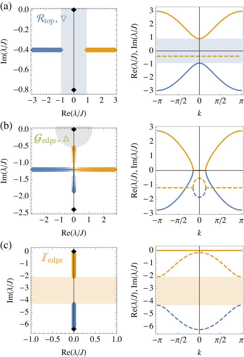
Figure 3: Liouvillian spectra for $J=\Delta=-\mu$ and $\gamma_{\mathrm{l}}=\gamma_{\mathrm{g}}=\gamma$. (a) Real line gap in the phase $\mathcal{R}_{\mathrm{top}}$ at weak dissipation with $\gamma=0.2J$. Left panel: Spectra for an infinite bulk system and a system with $N=100$ with open boundary conditions. The blue and orange solid lines that correspond to the bulk system are hidden behind the diamond symbols that indicate the eigenvalues of the finite system. Black diamonds at approximately $\lambda_{L}=-\mathrm{i}4\gamma$ and $\lambda_{R}=0$ are edge modes that are exponentially localized at the left and right edges, respectively van Caspel et al. (2019). All other modes are delocalized. Right panel: Real and imaginary parts of $\lambda_{\pm,k}$ in Eq. (IV) are shown as solid and dashed lines, respectively. (b) Gapless spectrum in the phase $\mathcal{G}_{\mathrm{edge}}$ at $\gamma=0.6J$. The gray disk indicates the point gap at $\lambda=0$. (c) Imaginary line gap in $\mathcal{I}_{\mathrm{edge}}$ at strong dissipation with $\gamma=1.6J$.

Since the eigenvalues of the Liouvillian are complex, gapped and gapless phases can be defined by addressing two distinct questions. First, we can ask whether the two bands $\lambda_{\pm,k}$ are separated in the complex plane. This question leads to the definition of real and imaginary line gaps Kawabata et al. (2019) as specified below. Further, for a complex spectrum, the point at which two bands touch in a gapless phase does not have to be $\lambda=0$. Therefore, we can introduce another notion of a spectral gap by asking: Is $\lambda=0$ contained in the spectrum of $z_{k}$? If this is not the case, the system has a point gap at $\lambda=0$ Kawabata et al. (2019). As we detail below and in Sec. V, closings of the two types of gaps, i.e., real or imaginary line gaps that separate the bands in the complex plane, or the point gap that separates both bands from $\lambda=0$, are associated with different types of topological transitions and leave distinct signatures, in particular, in the dynamics of the system.

We first discuss real and imaginary line gaps. If the expression under the square root in Eq. (IV) is positive for all values of $k$, the bands are separated along the real axis by a real line gap, which is indicated by the blue shading in Fig. 3(a). In the phase diagram in Fig. 2, a real line gap occurs in the phases $\mathcal{R}_{\mathrm{top}}$ and $\mathcal{R}_{\mathrm{tr}}$, in which the rates of dissipation are bounded by

$$2\sqrt{\gamma_{\mathrm{l}}\gamma_{\mathrm{g}}}<\min\{\left\lvert 2J+\mu\right\rvert,\left\lvert 2J-\mu\right\rvert\}.$$ (17)

If the rates $\gamma_{\mathrm{l}}$ and $\gamma_{\mathrm{g}}$ are increased beyond this bound, the system enters one of the two gapless phases, which are denoted by $\mathcal{G}_{\mathrm{edge}}$ and $\mathcal{G}_{\mathrm{tr}}$. In these phases, the spectrum features exceptional points at momenta $\pm k_{*}$, at which the expression under the square root in Eq. (IV) vanishes and thus the eigenvalues and the corresponding eigenvectors of $z_{k}$ coincide. This is exemplified in Fig. 3(b). Finally, at strong dissipation, when the expression under the square root in Eq. (IV) is negative for all values of $k$, the bands are separated by an imaginary line gap as indicated by the orange shading in Fig. 3(c). The corresponding phases $\mathcal{I}_{\mathrm{edge}}$ and $\mathcal{I}_{\mathrm{tr}}$ are delineated by

$$2\sqrt{\gamma_{\mathrm{l}}\gamma_{\mathrm{g}}}>\max\{\left\lvert 2J+\mu\right\rvert,\left\lvert 2J-\mu\right\rvert\}.$$ (18)

A non-Hermitian winding number $W$ for a single band can be defined only in the gapped phases, where the bands are separated, and the definition depends on the symmetries of the model. The driven-dissipative Kitaev chain belongs to class $\mathrm{BDI}^{\dagger}$ in the nomenclature of Ref. Kawabata et al. (2019), and obeys the following forms of time-reversal, particle-hole, and chiral symmetries:

TRS^†: $$\sigma_{z}z_{k}^{{\mathchoice{\raisebox{0.0pt}{$\displaystyle\intercal$}}{\raisebox{0.0pt}{$\textstyle\intercal$}}{\raisebox{0.0pt}{$\scriptstyle\intercal$}}{\raisebox{0.0pt}{$\scriptscriptstyle\intercal$}}}}\sigma_{z} =z_{-k},$$ (19)

PHS^†: $$z_{k}^{*} =-z_{-k},$$

CS: $$\sigma_{z}z_{k}^{\dagger}\sigma_{z} =-z_{k}.$$

For $\gamma_{\mathrm{l}}=\gamma_{\mathrm{g}}=0$, when $z_{k}=z_{k}^{\dagger}$, the class $\mathrm{BDI}^{\dagger}$ reduces to the class BDI of the isolated Hermitian Kitaev chain (1) with $\Delta\in\mathbb{R}$. The definition of the winding number $W$ for a single band of the isolated system can be generalized to the entire phases $\mathcal{R}_{\mathrm{top}}$ and $\mathcal{R}_{\mathrm{tr}}$ with a real line gap Kawabata et al. (2019). In Ref. Esaki et al. (2011), the calculation of $W$ for the shifted matrix $\tilde{z}_{k}$ in Eq. (16) is carried out, and leads to the result $W=1$ in the topological phase $\mathcal{R}_{\mathrm{top}}$ with $\left\lvert\mu\right\rvert<2J$, and $W=0$ in the trivial phase $\mathcal{R}_{\mathrm{tr}}$ with $\left\lvert\mu\right\rvert>2J$. As we show in Sec. V, non-Hermitian topology as characterized by the winding number $W=1$ for an individual band is reflected in the presence of entanglement spectrum crossings in quench dynamics. In contrast to the phases $\mathcal{R}_{\mathrm{top}}$ and $\mathcal{R}_{\mathrm{tr}}$ with a real line gap, the topology of individual bands of the Liouvillian is always trivial in the phases $\mathcal{I}_{\mathrm{edge}}$ and $\mathcal{I}_{\mathrm{tr}}$ with an imaginary line gap Kawabata et al. (2019). Consistently, we observe no entanglement spectrum crossings for quenches into $\mathcal{I}_{\mathrm{edge}}$ and $\mathcal{I}_{\mathrm{tr}}$.

A topological classification of the gapless phases can be given in terms of a global invariant, which is not a property of individual bands, but rather of the entire Liouvillian. In particular, the global Berry phase $Q$ defined and calculated for the shifted matrix $\tilde{z}_{k}$ in Eq. (16) in Ref. Liang and Huang (2013), takes the values $Q=1$ for $\left\lvert\mu\right\rvert<2J$ and $Q=0$ for $\left\lvert\mu\right\rvert>2J$. We stress that the global Berry phase $Q$ is defined in the entire phase diagram in Fig. 2, including the gapless phases $\mathcal{G}_{\mathrm{edge}}$ and $\mathcal{G}_{\mathrm{tr}}$. In contrast, the classification in terms of the non-Hermitian winding number $W$ applies only to the phases with real line gaps.

In the driven-dissipative Kitaev chain, a nonzero value of $Q$ implies the existence of edge modes Lieu (2018) even within the gapless phase $\mathcal{G}_{\mathrm{edge}}$ and the phase $\mathcal{I}_{\mathrm{edge}}$ with an imaginary line gap van Caspel et al. (2019), and not only in $\mathcal{R}_{\mathrm{top}}$. Edge modes are shown in the spectra in Fig. 3 as black diamonds. A topological transition occurs at the boundaries between $\mathcal{G}_{\mathrm{edge}}$ and $\mathcal{G}_{\mathrm{tr}}$ as well as $\mathcal{I}_{\mathrm{edge}}$ and $\mathcal{I}_{\mathrm{tr}}$, in which edge modes disappear because the value of $Q$ changes from $Q=1$ to $Q=0$. In crossing this transition, and when $\gamma_{\mathrm{l}}=\gamma_{\mathrm{g}}$, the second type of band gap defined above, i.e., the point gap at $\lambda=0$, closes. In Fig. 3(b), the point gap is indicated with a gray disk. Closings of this gap induce critical power-law relaxation in the dynamics of both the entanglement spectrum and response functions, as we discuss in Sec. V below.

V Systems with Hermitian jump operators

The definition of a non-Hermitian winding number $W$ for complex bands $\lambda_{\pm,k}$, which we discussed in Sec. IV, is purely formal, and raises the question about its physical implications. In the following, we show that the topological transition in the spectrum of the Liouvillian, in which $W$ changes from $W=1$ in $\mathcal{R}_{\mathrm{top}}$ to $W=0$ or undefined in $\mathcal{R}_{\mathrm{tr}}$ and $\mathcal{G}_{\mathrm{edge}}$, respectively, is associated with a dynamical phase transition in the time evolution of the entanglement spectrum.

We begin by introducing the tools which are required to track the time evolution of the entanglement spectrum, and which have been used to establish the entanglement spectrum bulk-edge correspondence in quench dynamics of isolated Hermitian systems Gong and Ueda (2018); Chang (2018); Lu and Yu (2019). Then, as one of the key results of our work, we generalize the entanglement spectrum bulk-edge correspondence to the driven-dissipative Kitaev chain.

In this section, we consider the effective Schrödinger equation (10) with a non-Hermitian matrix $Z=-\mathrm{i}X^{{\mathchoice{\raisebox{0.0pt}{$\displaystyle\intercal$}}{\raisebox{0.0pt}{$\textstyle\intercal$}}{\raisebox{0.0pt}{$\scriptstyle\intercal$}}{\raisebox{0.0pt}{$\scriptscriptstyle\intercal$}}}}$ and $Y=0$, which corresponds to Hermitian jump operators, i.e., $\gamma_{\mathrm{l}}=\gamma_{\mathrm{g}}=\gamma$ in Eq. (4). We discuss the general case with $\gamma_{\mathrm{l}}\neq\gamma_{\mathrm{g}}$ and thus $Y\neq 0$ in Sec. VI.

A distinguishing feature of systems with Hermitian jump operators is that they generically heat up to a fully mixed infinite-temperature state, $\rho_{\mathrm{ss}}=\rho_{\infty}=\mathbbm{1}/D$, where $D$ is the Hilbert-space dimension. This can be seen by noting that for $L_{i}=L_{i}^{\dagger}$, the dissipator in Eq. (3) takes the form of a double commutator,

$$\hat{\mathcal{D}}\rho=-\sum_{i=1}^{N}[L_{i},[L_{i},\rho]].$$ (20)

Therefore, the trivial state $\rho_{\infty}=\mathbbm{1}/D$, which satisfies $[H,\rho_{\infty}]=[L_{i},\rho_{\infty}]=0$, is indeed a steady state. Typically, this steady state is also unique. Degeneracy of the steady state requires the existence of at least two zero modes of the matrix $Z$ van Caspel et al. (2019); Lieu (2019). For the driven-dissipative Kitaev chain with Hermitian jump operators, the spectra in Fig. 3 display only a single zero mode which is localized at the right edge of the chain. Thus, $\rho_{\mathrm{ss}}=\rho_{\infty}$ is the unique steady state.

V.1 Topology from quench dynamics

To explore the dynamical topology of the driven-dissipative Kitaev chain, we study the time evolution of a pure state $\lvert\psi_{0}\rangle$, the ground state of the isolated Kitaev chain, after sudden changes of parameters. The quench protocol is illustrated in Fig. 1: At time $t=0^{+}$, the chemical potential is varied abruptly from its prequench value $\mu_{0}$ to a postquench value $\mu_{1}$, and at the same time the system is connected to Markovian baths.

Due to the coupling to Markovian baths, described by the term $\hat{\mathcal{D}}\rho$ in Eq. (2), the pure initial state $\rho_{0}=\lvert\psi_{0}\rangle\langle\psi_{0}\rvert$ evolves into a mixed state $\rho(t)=\mathrm{e}^{\hat{\mathcal{L}}t}\rho_{0}$. Since $H$ and $\hat{\mathcal{L}}$ are quadratic, both the initial ground state and the time-evolved density matrix $\rho(t)$ are Gaussian states, i.e., they can be written as the exponential of a quadratic form in the fermionic operators $c_{i}$ and $c_{i}^{\dagger}$. Gaussian states are fully determined by the real and antisymmetric covariance matrix Campbell (2015); Bravyi and König (2012),

$$\Gamma_{i,j}(t)=\frac{\mathrm{i}}{2}\mathop{\mathrm{tr}}([w_{i},w_{j}]\rho(t)).$$ (21)

The covariance matrix obeys the equation of motion $\mathrm{d}\Gamma/\mathrm{d}t=-X\Gamma-\Gamma X^{{\mathchoice{\raisebox{0.0pt}{$\displaystyle\intercal$}}{\raisebox{0.0pt}{$\textstyle\intercal$}}{\raisebox{0.0pt}{$\scriptstyle\intercal$}}{\raisebox{0.0pt}{$\scriptscriptstyle\intercal$}}}}-Y$, which is solved by Prosen and Ilievski (2011)

$$\Gamma(t)=\mathrm{e}^{-Xt}\left(\Gamma(0)-\int_{0}^{t}\mathrm{d}t^{\prime}\,\mathrm{e}^{Xt^{\prime}}Y\mathrm{e}^{X^{{\mathchoice{\raisebox{0.0pt}{$\displaystyle\intercal$}}{\raisebox{0.0pt}{$\textstyle\intercal$}}{\raisebox{0.0pt}{$\scriptstyle\intercal$}}{\raisebox{0.0pt}{$\scriptscriptstyle\intercal$}}}}t^{\prime}}\right)\mathrm{e}^{-X^{{\mathchoice{\raisebox{0.0pt}{$\displaystyle\intercal$}}{\raisebox{0.0pt}{$\textstyle\intercal$}}{\raisebox{0.0pt}{$\scriptstyle\intercal$}}{\raisebox{0.0pt}{$\scriptscriptstyle\intercal$}}}}t}.$$ (22)

Here, $\Gamma(0)$ is the covariance matrix of the initial state. As stated above, we assume that the system is prepared in the ground state of the isolated Kitaev chain, and the corresponding covariance matrix is elaborated in Appendix B. For $Y=0$, the second term in Eq. (22) vanishes, and $\Gamma(t)$ decays to zero in the steady state $\rho_{\mathrm{ss}}=\rho_{\infty}=\mathbbm{1}/D$.

In the following, we assume that the number of lattice sites $N$ is even, and we consider an equal bipartition of the system into its left and right halves. There are in total $2N$ sites of Majorana fermions. We denote the set of site indices of Majorana fermions which belong to the left half of the system by $A=\{1,\dotsc,N\}$. Then, the reduced covariance matrix of subsystem $A$ is defined as $\Gamma_{i,j}^{A}=\left(\Gamma_{i,j}\right)_{i,j\in A}$. Its eigenvalues, which come in pairs $\pm\xi_{i}$ of bounded values $0\leq\xi_{i}\leq 1$ with $i=1,\dotsc,N/2$, form the single-particle entanglement spectrum Cheong and Henley (2004); Peschel and Eisler (2009); Kraus et al. (2009).

For Gaussian states, the equality $\xi_{i}=\tanh(\varepsilon_{i}/2)$ relates the entanglement eigenvalues $\xi_{i}$ to the single-particle eigenvalues $\varepsilon_{i}$ of the entanglement Hamiltonian $H_{A}$, which is determined by the reduced density matrix as $\rho_{A}={\mathop{\mathrm{tr}}}_{A^{\mathrm{c}}}(\rho)=\mathrm{e}^{-H_{A}}/Z_{A}$ where $Z_{A}={\mathop{\mathrm{tr}}}_{A}(\mathrm{e}^{-H_{A}})$ Cheong and Henley (2004); Peschel and Eisler (2009); Kraus et al. (2009). The many-body entanglement spectrum, which is defined as the spectrum of $\rho_{A}$, is thus given by Fidkowski (2010)

$$\Xi_{\mathbf{e}}=\prod_{i=1}^{N/2}\frac{1}{2}\left[1+\left(-1\right)^{e_{i}}\xi_{i}\right],$$ (23)

where $\mathbf{e}=\left(e_{1},\dotsc,e_{N/2}\right)$, and where the numbers $e_{i}$ are to be understood as occupations of single-particle entanglement levels that take the values $e_{i}=0,1$. Therefore, for Gaussian states, the single-particle and many-body entanglement spectra contain the same information. In particular, as detailed below, Eq. (23) implies that a zero crossing in the single-particle entanglement spectrum leads to the simultaneous crossing of pairs of many-body entanglement eigenvalues.

V.1.1 time evolution of entanglement spectra

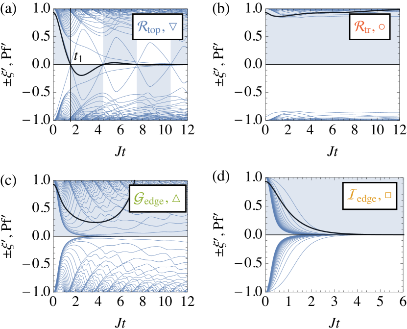
Figure 4: Time evolution of entanglement spectra. Rescaled single-particle entanglement spectrum, $\xi^{\prime}=\xi\mathrm{e}^{4\gamma t}$, for a quench from the trivial phase at $\mu_{0}=-3J$ to (a) the topological phase $\mathcal{R}_{\rm top}$ with $W=1$ at $\mu_{1}=-J$ and $\gamma=0.2J$, (b) the trivial phase $\mathcal{R}_{\mathrm{tr}}$ with $W=0$ at $\mu_{1}=-2.5J$ and $\gamma=0.1J$, (c) the gapless phase $\mathcal{G}_{\mathrm{edge}}$ at $\mu_{1}=-J$ and $\gamma=0.6J$, and (d) the trivial phase $\mathcal{I}_{\mathrm{edge}}$ at $\mu_{1}=0$ and $\gamma=1.1J$. Zero crossings in the entanglement spectrum, which occur in (a) but not in (b–d), are tracked by the rescaled Pfaffian, $\mathrm{Pf}^{\prime}=\mathop{\mathrm{Pf}}\mathrm{e}^{4\gamma Nt}$, which is shown as a black solid line. The sign of the Pfaffian is indicated by the blue shading. The parameters in (a), (b), (c), and (d) correspond, respectively, to the blue inverted triangle, red circle, green triangle, and orange square in Fig. 2.

Before we continue, it is instructive to recall previous results for isolated systems. Notably, Gong and Ueda Gong and Ueda (2018) connected the occurrence of entanglement spectrum crossings in the quench dynamics and the topology of the prequench and postquench Hamiltonians, $H_{0}$ and $H$, respectively, of a one-dimensional isolated system. Their key observation is that the time-evolved state $\lvert\psi(t)\rangle=\mathrm{e}^{-\mathrm{i}Ht}\lvert\psi_{0}\rangle$, where $\lvert\psi_{0}\rangle$ is the ground state of $H_{0}$, is the ground state of a time-dependent parent Hamiltonian defined as $H_{\mathrm{p}}(t)=\mathrm{e}^{-\mathrm{i}Ht}H_{0}\mathrm{e}^{\mathrm{i}Ht}$. If $H$ is assumed to be band-flattened, the time dependence of $H_{\mathrm{p}}(t)$ is periodic, and, therefore, in the first-quantized Hamiltonian $H_{\mathrm{p}}(k,t)$, the time $t$ can be interpreted as a second quasimomentum variable. By virtue of the entanglement spectrum bulk-edge correspondence, the evolution of the entanglement spectrum over one period gives the exact edge spectrum of the $(1+1)$-dimensional band-flattened Bloch Hamiltonian $H_{\mathrm{p}}(k,t)$ Fidkowski (2010). In particular, nontrivial topology of $H_{\mathrm{p}}(k,t)$ is reflected in the presence of entanglement edge modes which cross the band gap as a function of $t$. For the Altland-Zirnbauer classes in which nontrivial topology of $H_{\mathrm{p}}(k,t)$ is realized, the two-dimensional topological index of the parent Hamiltonian $H_{\mathrm{p}}(k,t)$ is the difference between the one-dimensional topological indices of $H_{0}$ and $H$ Gong and Ueda (2018). Therefore, entanglement spectrum crossings occur, in particular, for quenches from a trivial phase of $H_{0}$ to a topological phase of $H$, and serve as a proxy for nontrivial topology of $H$. As we discuss in the following, the connection between entanglement spectrum crossings and nontrivial topology of the generator of dynamics remains intact if, instead of unitary time evolution generated by a Hamiltonian $H$, we consider the driven-dissipative dynamics of an open quantum many-body system as described by the master equation (2) with a non-Hermitian superoperator $\hat{\mathcal{L}}$.

Throughout this section, we take the system to be initialized in the topologically trivial ground state of the isolated Kitaev chain with Hamiltonian (1), where $J=\Delta$ sets the energy scale. Our results do not depend qualitatively on the precise prequench value of the chemical potential. For concreteness, we choose $\mu_{0}=-3J$.

Figure 4(a) shows a quench to the non-Hermitian topological phase $\mathcal{R}_{\mathrm{top}}$ with $W=1$ at $\mu_{1}=-J$ and $\gamma=0.2J$. The parameters of the postquench Liouvillian are indicated with a blue inverted triangle in Fig. 2, and the spectrum of the Liouvillian for these parameters is shown in Fig. 3(a). As can be seen in the latter figure, the bulk modes, which are shown as blue and orange diamond symbols, decay with the same rate $-\mathop{\mathrm{Im}}(\lambda_{\mathrm{bulk}})=2\gamma=0.4J$. Then, for the covariance matrix, and, consequently, its eigenvalues which form the single-particle entanglement spectrum, Eq. (22) implies a decay rate of $4\gamma=0.8J$. To best illustrate the evolution of the entanglement spectrum in Fig. 4, we account for this overall decay by rescaling the entanglement eigenvalues as $\xi^{\prime}=\xi\mathrm{e}^{4\gamma t}$. With this rescalling, in Fig. 4(a), most of the single-particle entanglement eigenvalues, which are shown as blue lines, stay close to $\pm 1$. However, a pair of eigenvalues $\pm\xi_{i}^{\prime}$ undergoes repeated zero crossings. To trace these crossings, we employ the Pfaffian of the reduced covariance matrix,

$$\mathrm{Pf}(t)=\mathop{\mathrm{pf}}(\Gamma_{A}(t)).$$ (24)

The Pfaffian, which can be defined for any antisymmetric matrix, has the following properties: Its absolute value is given by the square root of the determinant, and, most importantly, it changes sign whenever a pair of entanglement eigenvalues $\pm\xi_{i}$ crosses zero. In all panels of Fig. 4, the rescaled Pfaffian $\mathrm{Pf}^{\prime}=\mathop{\mathrm{Pf}}\mathrm{e}^{4\gamma Nt}$ is shown as a black line, and its sign is indicated with blue shaded areas. At long times, the covariance matrix (22), and, consequently, also the Pfaffian (24) decay to zero.

The entanglement spectrum crossings disappear when the postquench parameters are within a trivial phase in which $W=0$ or $W$ is undefined. Figure 4(b) shows the entanglement spectrum dynamics following a quench to the real-line gapped trivial phase $\mathcal{R}_{\mathrm{tr}}$ with $W=0$ at $\mu_{1}=-2.5J$ and $\gamma=0.1J$, as indicated by the red circle in Fig. 2. As above, the decay rates of all bulk modes are equal to $2\gamma$. Therefore, rescaling the entanglement eigenvalues with $\mathrm{e}^{4\gamma t}$ removes the overall decay of the entanglement spectrum and leaves all entanglement eigenvalues close to $\pm 1$.

The evolution of the entanglement spectrum shows richer phenomenology for quenches to the gapless phases $\mathcal{G}_{\mathrm{edge}}$ and $\mathcal{G}_{\mathrm{tr}}$, in which the winding number $W$ is undefined. Figure 4(c) shows a quench to the phase $\mathcal{G}_{\mathrm{edge}}$ at $\mu_{1}=-J$ and $\gamma=0.6J$, as indicated by the green triangle in Fig. 2. The corresponding spectrum of the postquench Liouvillian is shown in Fig. 3(b). Decay rates of bulk modes are within a finite range of values, and, therefore, the rescaling of the entanglement spectrum with $\mathrm{e}^{4\gamma t}$ leads to the occurrence of exponentially growing values. Thus, the rescaled Pfaffian in Fig. 4(c) soon exceeds one. Crucially, and in agreement with the fact that in a gapless phase the postquench Liouvillian is not characterized by a nontrivial non-Hermitian winding number, the Pfaffian does not change sign.

Figure 4(d) presents the time evolution of the entanglement spectrum after a quench to the imaginary-line gapped phase $\mathcal{I}_{\mathrm{edge}}$ at $\mu_{1}=0$ and $\gamma=1.1J$, as indicated by the orange square in Fig. 2. For these postquench parameters, the two bands (IV) are purely imaginary as shown in Fig. 3(c). This is reflected vividly in the purely decaying behaviour of the entenglement spectrum.

We proceed with a quantitative analysis of the time evolution of the entanglement spectrum for quenches to the topological phase $\mathcal{R}_{\mathrm{top}}$. The color scale within the phase $\mathcal{R}_{\mathrm{top}}$ in Fig. 2 encodes the time $t_{1}$ at which the first zero crossing in the single-particle entanglement spectrum occurs. In Fig. 4(a), the time $t_{1}$ is indicated with a vertical black line. The values of $t_{1}$ diverge at the boundaries of the phase $\mathcal{R}_{\mathrm{top}}$. This is illustrated in the inset of Fig. 2, where $t_{1}$ is shown for variations of the parameters of the postquench Liouvillian along the black arrows in the main panel of the figure, i.e., for $\delta\mu=\mu_{1}+2J\to 0$ and $\gamma=0$, and for $\mu_{1}=-J$ and $\delta\gamma=0.5J-\gamma\to 0$, respectively. The numerical data is consistent with a square-root singularity, which is shown as a gray line in the inset of Fig. 2, and which corresponds to the behavior $t_{1}\sim\delta\mu^{-\epsilon}$ and $t_{1}\sim\delta\gamma^{-\epsilon}$, where $\epsilon=1/2$ can be interpreted as a dynamical critical exponent for entanglement spectrum crossings. In Sec. V.1.2, we show that the value $\epsilon=1/2$ is exact for the specific case of a postquench Liouvillian with flat spectrum, in which an exact solution of the quench dynamics is possible. In the numerical data shown in the inset of Fig. 2, the singularity of $t_{1}$ is cut due to the finite system size. The values of $t_{1}$ saturate earlier if the phase boundary is approached by varying the strength of dissipation.

The singularity of $t_{1}$ at the boundaries of the topological phase $\mathcal{R}_{\mathrm{top}}$ raises the question, whether the time evolution of the entanglement spectrum exhibits also other signatures of dynamical criticality. To complement our analysis of oscillatory behavior of entanglement eigenvalues, which is characterized by the time scale $t_{1}$, we illustrate in Fig. 5 the decay of the largest eigenvalue $\xi_{\mathrm{max}}$. It exhibits critical power-law relaxation at the phase boundary between the gapless phases $\mathcal{G}_{\mathrm{edge}}$ and $\mathcal{G}_{\mathrm{tr}}$, where the global Berry phase jumps from $Q=1$ to $Q=0$ and, concomitantly, the edge modes of the Liouvillian disappear. This form of decay is also realized generically for quenches in isolated Hermitian systems Jhu et al. (2017). However, the decay of $\xi_{\mathrm{max}}$ follows a simple exponential form across the boundary between $\mathcal{R}_{\mathrm{top}}$ and $\mathcal{G}_{\mathrm{edge}}$.

Figure 5: Relaxation dynamics of the largest entanglement eigenvalue $\xi_{\mathrm{max}}$. (a) Exponential decay across the phase boundary between $\mathcal{R}_{\mathrm{top}}$ and $\mathcal{G}_{\mathrm{edge}}$ at $\mu_{1}=-J$ and for three values of $\gamma$ below, at, and above the critical value $\gamma_{\mathrm{c}}=0.5J$. (b) The decay $\Gamma_{\mathrm{max}}$ of $\xi_{\mathrm{max}}$ exhibits a maximum at the phase boundary. The numerically determined value of $\Gamma_{\mathrm{max}}$ is shown as an orange dashed line, and the blue solid line corresponds to the analytical expression (25). (c) Critical relaxation of $\xi_{\mathrm{max}}$ at the phase boundary between $\mathcal{G}_{\mathrm{edge}}$ and $\mathcal{G}_{\mathrm{tr}}$ at $\gamma=J$ and for values of $\mu_{1}$ ranging from $\mu_{1}=-J$ to the critical value $\mu_{1}=-2J$, shown as red to blue lines. For comparison, power-law behavior $\xi_{\mathrm{max}}\sim\left(Jt\right)^{-1/2}$ is shown as a gray line.

In particular, in Fig. 5(a) we show the decay of $\xi_{\mathrm{max}}$ for three different values of the rate of dissipation $\gamma$ below, at, and above the critical value $\gamma_{\mathrm{c}}=0.5J$ for $\mu_{1}=-J$. For each value of $\gamma$, the approximately linear behavior of $\xi_{\mathrm{max}}$ on the semilogarithmic scale indicates dominantly exponential relaxation. Indeed, we find good agreement of the numerical data with $\xi_{\mathrm{max}}\sim\mathrm{e}^{-\Gamma_{\mathrm{max}}t}$ and $\xi_{\mathrm{max}}\sim\mathrm{e}^{-\Gamma_{\mathrm{max}}t}/\sqrt{t}$ for $\gamma<\gamma_{\mathrm{c}}$ and $\gamma>\gamma_{\mathrm{c}}$, respectively. The numerically determined decay rate $\Gamma_{\mathrm{max}}$ is shown as a function of $\gamma$ in Fig. 5(b). It agrees well with the analytical expression

$$\Gamma_{\mathrm{max}}=\begin{cases}4\gamma&\text{for }\gamma<\gamma_{\mathrm{c}},\\ 2\left(2\gamma-\sqrt{4\gamma^{2}-\left(2J+\mu_{1}\right)^{2}}\right)&\text{for }\gamma>\gamma_{\mathrm{c}},\end{cases}$$ (25)

which is inspired by the exact result for the decay rate of the retarded response function as elaborated in Sec. V.2 below. Interestingly, $\Gamma_{\mathrm{max}}$ takes a maximum value of $\Gamma_{\mathrm{max}}=2J$ exactly at the critical point $\gamma=\gamma_{\mathrm{c}}=0.5J$. This observation runs counter to the common expectation that relaxation to the steady state becomes exceedingly slow in the vicinity of a phase transition. In Sec. V.2, we explain this unusual behavior through a mechanism of many-body critical damping.

The dynamics of the entanglement spectrum exhibits rather different behavior across the boundary between $\mathcal{G}_{\mathrm{edge}}$ and $\mathcal{G}_{\mathrm{tr}}$. As discussed above, there is no qualitative change in the oscillatory dynamics: For quenches to both $\mathcal{G}_{\mathrm{edge}}$ and $\mathcal{G}_{\mathrm{tr}}$, there are no zero crossings of entanglement eigenvalues. However, as illustrated in Fig. 5(c), the decay of the largest entanglement eigenvalue $\xi_{\mathrm{max}}$ shows critical slowing down as the phase boundary is approached, and power-law relaxation $\xi_{\mathrm{max}}\sim\left(Jt\right)^{-1/2}$ exactly on the phase boundary. The origin of this behavior is the closing of the point gap at $\lambda=0$. We provide a quantitative analysis of dynamical criticality in terms of two-time correlation functions in Sec. V.2.

V.1.2 Driven-dissipative fermion parity pump

We proceed to complement our numerical results for the time evolution of entanglement spectra with an exact analytical solution, which is enabled by a judicious choice of the initial state and the parameters of the postquench Liouvillian. First, this provides us with an interpretation of topological quench dynamics as a fermion parity pump; and second, for specific parameter values, we are able to show explicitly that the entanglement spectrum dynamical critical exponent takes the exact value $\epsilon=1/2$.

To facilitate analytical progress, we assume that the system is initialized in the vacuum of Dirac fermions $c_{i}$, which is the ground state of the Hamiltonian of the Kitaev chain for $J=\Delta>0$ and $\mu_{0}\to-\infty$. Further, we choose the parameters of the postquench Liouvillian as $J=\Delta>0$, $\mu_{1}=0$, and $\gamma_{\mathrm{l}}=\gamma_{\mathrm{g}}=\gamma$. For this choice of postquench parameters, the bulk spectrum (IV) for an infinite chain becomes flat with

$$\lambda_{\pm}=2\left(-\mathrm{i}\gamma\pm\sqrt{J^{2}-\gamma^{2}}\right).$$ (26)

The spectrum exhibits a real line gap when $\gamma<\gamma_{\mathrm{c}}=J$, and the expression under the square root is positive. In contrast, for $\gamma>J$, the two flat bands are separated by an imaginary line gap.

For a Liouvillian with flat bulk bands, also the spectrum for an open finite chain of length $N$ can be obtained analytically, and is given by $\{\lambda_{\pm},\lambda_{L},\lambda_{R}\}$. In a finite system, the values $\lambda_{\pm}$ given in Eq. (26) have degeneracy $N-1$ each, and $\lambda_{L}=-\mathrm{i}4\gamma$ and $\lambda_{R}=0$ are eigenvalues corresponding to edge modes which are localized on the left and the right end of the chain, respectively. For $\gamma<J$, the real part of the eigenvalues $\lambda_{\pm}$ sets a time scale,

$$T=\pm\frac{\pi}{\mathop{\mathrm{Re}}(\lambda_{\pm})}=\frac{\pi}{2\sqrt{J^{2}-\gamma^{2}}},$$ (27)

for oscillations of the bulk modes. As we show in the following, this is the time scale on which the fermion parity of many-body entanglement eigenstates is reversed and, concomitantly, both single-particle and many-body entanglement eigenvalues cross. More precisely, as illustrated in Fig. 6 where the times $mT$, with $m\in\mathbb{N}_{0}$ a nonnegative integer, are indicated with green vertical lines, entanglement spectrum crossings occur at times $t_{m}$ which obey $mT<t_{m}<\left(m+1\right)T$.

The key result, based on which we establish the connection between entanglement spectrum crossings and the reversal of the fermion parity at the edges of the Kitaev chain, is an exact expression for the reduced density matrix $\rho_{A}(mT)$ at times $t=mT$ with $m\in\mathbb{N}_{0}$, which we derive in Appendix C. As we show there, for the choice of initial state and postquench Liouvillian specified above, the reduced density matrix $\rho_{A}(mT)$ is diagonal in a basis of Fock states with fixed number of particles on each lattice site, which we denote by $\lvert\mathbf{n}\rangle_{A}$ where $\mathbf{n}=\left(n_{1},\dotsc,n_{N/2}\right)$ is a vector of lattice-site occupation numbers with $n_{i}=0,1$. In terms of projectors $P^{\mathbf{n}}=\lvert\mathbf{n}\rangle_{A}\langle\mathbf{n}\rvert$ on these basis states, the reduced density matrix can be written as

$$\rho_{A}(mT)=\sum_{\mathbf{e}}\Xi_{\mathbf{e},m}P^{\mathbf{n}_{\mathbf{e},m}},$$ (28)

where the sum is over all combinations $\mathbf{e}=\left(e_{1},\dotsc,e_{N/2}\right)$ of single-particle entanglement occupation numbers $e_{i}=0,1$, and the coefficients $\Xi_{\mathbf{e},m}$ are the eigenvalues of $\rho_{A}(mT)$ and determine the many-body entanglement spectrum. We specify the relation between the lattice-site occupation numbers $\mathbf{n}_{\mathbf{e},m}$ and the entanglement occupation numbers $\mathbf{e}$ below.

For the exact solution (28) derived in Appendix C, the many-body entanglement eigenvalues $\Xi_{\mathbf{e},m}$ take the general form given in Eq. (23), with only two distinct single-particle entanglement eigenvalues,

$$\xi_{1,m}=\mathrm{e}^{-6\gamma mT},\qquad\xi_{2,m}=\mathrm{e}^{-4\gamma mT}.$$ (29)

The first eigenvalue $\xi_{1,m}$ is nondegenerate, whereas $\xi_{2,m}$ has degeneracy $N/2-1$. Both single-particle entanglement eigenvalues decay exponentially with rates $6\gamma$ and $4\gamma$, respectively. The exact analytical results for $\pm\xi_{1,m}$ and $\pm\xi_{2,m}$ are shown, respectively, as black and red crosses in Fig. 6(a). We find perfect agreement with the numerically calculated entanglement spectrum $\{\pm\xi_{i}(t)\}$, which is indicated with blue lines, at times $t=mT$.

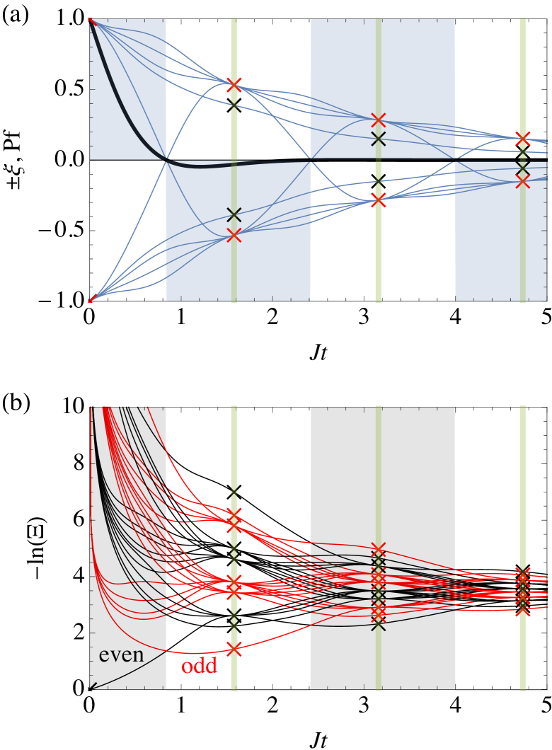
Figure 6: (a) Time evolution of the single-particle entanglement spectrum for a quench from $\mu_{0}\to-\infty$, to $\mu_{1}=0$, and $\gamma_{\mathrm{l}}=\gamma_{\mathrm{g}}=\gamma=0.1J$ for $N=10.$ The solid black line is the Pfaffian, and the blue shading indicates the sign of the Pfaffian. Green vertical lines mark integer multiples of the time scale $T$ in Eq. (27). Black and red crosses indicate, respectively, $\pm\xi_{1,m}$ and $\pm\xi_{2,m}$, for the analytical results given in Eq. (29). (b) Fermion parity pump illustrated with the evolution of the many-body entanglement spectrum for a quench with the same parameters as in (a). Black and red lines correspond to many-body entanglement eigenstates with even and odd parity, respectively. The parity of the entanglement ground state is even (odd) in the regions with (without) gray shading. Crosses indicate analytical results at multiples of $T$ marked by green vertical lines.

The reversal of the fermion parity at the ends of the chain is encoded in the relation between entanglement occupation numbers $\mathbf{e}$ and the site occupation numbers $\mathbf{n}_{\mathbf{e},m}$ in Eq. (28). As we show in Appendix C,

$$\mathbf{n}_{\mathbf{e},m}=\begin{cases}\mathbf{e}&\text{for $m$ even,}\\ \bar{\mathbf{e}}&\text{for $m$ odd,}\end{cases}$$ (30)

where vectors with an overbar are defined by $\bar{e}_{1}=(e_{1}+1)\bmod 2$, whereas $\bar{e}_{i}=e_{i}$ for $i=2,\dotsc,N/2$. That is, $\mathbf{e}$ and $\bar{\mathbf{e}}$ differ only in the first component.

To demonstrate the reversal of the fermion parity after each time step of duration $T$, we follow the evolution of the entanglement ground state, i.e., the state which corresponds to the smallest eigenvalue of the entanglement Hamiltonian $H_{A}$. According to the relation between the reduced density matrix $\rho_{A}$ and the entanglement Hamiltonian, $\rho_{A}=\mathrm{e}^{-H_{A}}/Z_{A}$ where $Z_{A}={\mathop{\mathrm{tr}}}_{A}(\mathrm{e}^{-H_{A}})$, the entanglement ground state is the eigenstate of $\rho_{A}$ with the largest many-body entanglement eigenvalue $\Xi_{\mathbf{e}}$ in Eq. (23). The latter equation implies that the largest many-body entanglement eigenvalue is obtained if all entanglement occupation numbers are equal to zero, $\mathbf{e}=\mathbf{0}$. The corresponding lattice-site occupation numbers (30) are $\mathbf{n}_{\mathbf{0},m}=\mathbf{0}$ for even values of $m$, and $\mathbf{n}_{\mathbf{0},m}=\bar{\mathbf{0}}=\left(1,0,\dotsc,0\right)$ for odd values of $m$. The entanglement ground state is thus given by $\lvert\mathbf{0}\rangle_{A}$ when $m$ is even, and by $\lvert\bar{\mathbf{0}}\rangle_{A}$ when $m$ is odd. These states have opposite fermion parity:

$$P_{A}\lvert\mathbf{0}\rangle_{A}=\lvert\mathbf{0}\rangle_{A},\qquad P_{A}\lvert\bar{\mathbf{0}}\rangle_{A}=-\lvert\bar{\mathbf{0}}\rangle_{A},$$ (31)

as follows directly from the definition of the fermion parity operator for subsystem $A$, i.e., the left half of the chain,

$$P_{A}=\mathrm{e}^{\mathrm{i}\pi\sum_{i=1}^{N/2}c_{i}^{\dagger}c_{i}}.$$ (32)

We proceed to connect the reversal of the fermion parity of the entanglement ground state to crossings in the many-body entanglement spectrum. Indeed, as we show in Appendix D, the entanglement eigenstates have definite parity at all times $t$. Therefore, a change of the fermion parity of the entanglement ground state between $t=mT$ and $t=\left(m+1\right)T$ implies that there is a crossing in the entanglement spectrum in which the entanglement ground state and the first excited state, which have opposite fermion parity, switch places. Numerically, as shown in Fig. 6(b), we find that there is exactly one crossing between the entanglement ground state and the first excited state, which occurs at a time $t_{m}$ in the interval $mT<t_{m}<\left(m+1\right)T$.

A crossing between the entanglement ground state and the first excited state in turn implies a zero crossing in the single-particle entanglement spectrum. To see this, we consider the difference between the entanglement eigenvalues of the ground state and first excited state. As we have already noted, the ground state corresponds to $\mathbf{e}=\mathbf{0}$. The first excited state is obtained by occupying the single-particle entanglement level with the smallest eigenvalues $\xi_{1}(t)$, where we order the single-particle entanglement eigenvalues $\xi_{i}(t)$ such that $0\leq\xi_{1}(t)\leq\dotsb\leq\xi_{N/2}(t)$. Thus, for the first excited state, the entanglement occupation numbers are $\mathbf{e}=\bar{\mathbf{0}}$. According to Eq. (23), which expresses the many-body entanglement spectrum in terms of the single-particle entanglement spectrum, the difference between the entanglement eigenvalues $\Xi_{\mathbf{0}}(t)$ and $\Xi_{\bar{\mathbf{0}}}(t)$ is given by

$$\Xi_{\mathbf{0}}(t)-\Xi_{\bar{\mathbf{0}}}(t)=\xi_{1}(t)\prod_{i=2}^{N/2}\frac{1}{2}\left(1+\xi_{i}(t)\right).$$ (33)

This difference is equal to zero when $\xi_{1}(t)=0$. That is, when the fermion parity for the many-body entanglement ground state is reversed, there is a zero crossing in the single-particle entanglement spectrum.

Interestingly, a zero crossing of $\xi_{1}(t)$ leads to simultaneous crossings of all pairs of many-body entanglement eigenstates with entanglement occupation numbers $\mathbf{e}$ and $\bar{\mathbf{e}}$. The difference between the corresponding entanglement eigenvalues is given by

$$\Xi_{\mathbf{e}}(t)-\Xi_{\bar{\mathbf{e}}}(t)=\left(-1\right)^{e_{1}}\xi_{1}(t)\prod_{i=2}^{N/2}\frac{1}{2}\left[1+\left(-1\right)^{e_{i}}\xi_{i}(t)\right],$$ (34)

and vanishes again when $\xi_{1}(t)=0$. Figures 6(a) and (b) illustrate this connection between zero crossings in the single-particle entanglement spectrum and simultaneous crossings of pairs of many-body entanglement eigenvalues. As can be seen in Fig. 6(b), there are further occasional crossings in the many-body entanglement spectrum that are not related to zero crossings in the single-particle entanglement spectrum, and which are not of topological origin.

Finally, we demonstrate numerically that the simultaneous crossings in the many-body entanglement spectrum occur between pairs of states which have opposite parity, and that, therefore, a zero crossing in the single-particle entanglement spectrum leads to the simultaneous reversal of the fermion parity in all entanglement eigenstates. To this end, we first note that according to Eq. (30), pairs of entanglement eigenstates with entanglement spectrum occupation numbers $\mathbf{e}$ and $\bar{\mathbf{e}}$ have opposite parity at times $t=mT$. As discussed in Appendix D, parity is conserved during the dynamics. We can thus track the parity of all entanglement eigenstates at all times, even without calculating the full many-body density matrix $\rho_{A}$. In Fig. 6(b), black and red lines correspond to even and odd parity, respectively. The parity of the entanglement ground state is even in regions with gray shading. At the boundaries of these regions, which agree with the boundaries of the blue-shaded regions in Fig. 6(a) that mark changes of the sign of the Pfaffian due to zero crossings in the single-particle entanglement spectrum, simultaneous crossings in the many-body entanglement spectrum occur between pairs of states with opposite parity.

The above considerations establish the interpretation of entanglement spectrum crossings as a fermion parity pump for a particular choice of parameters. In general, this interpretation remains valid for continuous variations of pre- and postquench parameters within the trivial phase of the isolated Kitaev chain and the non-Hermitian topological phase of the driven and open Kitaev chain, respectively. To convince oneself that this is the case, it is sufficient to note that, as detailed in Appendix D, fermion parity is always a good quantum number of entanglement eigenstates for the models and dynamics we consider here, i.e., quench dynamics starting from a state with definite parity, and where time evolution is generated by a quadratic Liouvillian.

The period $T$ of the fermion parity pump diverges when the rate of dissipation approaches the critical value of $\gamma_{\mathrm{c}}=J$. Specifically, by inserting $\delta\gamma=\gamma_{\mathrm{c}}-\gamma$ in Eq. (27), we obtain

$$T\sim\frac{\pi}{2J\sqrt{2\delta\gamma/J}},\quad\delta\gamma\searrow 0.$$ (35)

Consequently, also the times $t_{m}$ at which entanglement spectrum crossings occur exhibit a square-root singularity, $t_{m}\sim\delta\gamma^{-\epsilon}$ with $\epsilon=1/2$. In the inset of Fig. 2, we present numerical evidence for the universality of the value of the entanglement spectrum critical exponent $\epsilon$. In particular, our numerical results indicate that $\epsilon=1/2$ when we (i) consider dispersive bands of the postquench Liouvillian, (ii) approach the phase boundary of $\mathcal{R}_{\mathrm{top}}$ from different directions, by tuning either $\gamma$ or $\mu_{1}$, (iii) consider a more general topologically trivial initial state with $J,\Delta\neq 0$ and $2J<\left\lvert\mu_{0}\right\rvert<\infty$, i.e., a trivial state that is different from the vacuum of Dirac fermions, and (iv) study different models such as the one with quasilocal jump operators defined in Eq. (5) and discussed in detail in Appendix A.

V.2 Dynamical critical behavior

In Sec. V.1.1, we have encountered two distinct types of dynamical critical behavior of the entanglement spectrum: the time $t_{1}$ of the first entanglement spectrum crossing diverges with an exponent $\epsilon=1/2$ at the boundary of $\mathcal{R}_{\mathrm{top}}$, while the relaxation of the largest entanglement eigenvalue $\xi_{\mathrm{max}}$ follows a simple exponential form across the phase boundary; In contrast, there are no entanglement spectrum crossings on both sides of the phase boundary between $\mathcal{G}_{\mathrm{edge}}$ and $\mathcal{G}_{\mathrm{tr}}$. However, $\xi_{\mathrm{max}}$ exhibits critical power-law relaxation exactly at this phase boundary. In the following, we show that a unified perspective on these different forms of dynamical criticality can be obtained by studying two-time correlation functions.

We consider the Keldysh Green’s function, together with the retarded and advanced response functions Sieberer et al. (2016), in terms of which all two-time correlation functions can be specified:

$$\chi^{K}_{i,j}(t) =-\frac{\mathrm{i}}{2}\langle[w_{i}(t),w_{j}]\rangle,$$ (36)

$$\chi^{R}_{i,j}(t) =\frac{1}{2}\theta(t)\langle\{w_{i}(t),w_{j}\}\rangle,$$ (37)

$$\chi^{A}_{i,j}(t) =\frac{1}{2}\theta(-t)\langle\{w_{i}(t),w_{j}\}\rangle,$$ (38)

where $\theta(t)$ is the Heaviside step function. We omit the usual factors $\mp\mathrm{i}$ in the definitions of the retarded and advanced response functions to obtain real-valued quantities. The expectation values are taken in the steady state $\rho_{\mathrm{ss}}$ and, therefore, it is sufficient to include a single time argument since two-time averages depend only on the time difference. For dynamics described by a master equation in Lindblad form, two-time averages can be calculated with the aid of the quantum regression theorem Gardiner and Zoller (2014) as detailed in Appendix E. Further, we assume here an infinite bulk system such that the correlation functions are translationally invariant.

The two-time correlation functions defined above are distinguished from the covariance matrix Eq. (21) in two aspects: first, the expectation value is taken in the steady state $\rho_{\mathrm{ss}}$ in the two-time correlation functions, and not in the time-dependent state $\rho(t)=\mathrm{e}^{\mathcal{L}t}\rho_{0}$ as in the case of the covariance matrix; second, here the Majorana operators $w_{i}$ and $w_{j}$ are evaluated at different times. In the limit $t\to\infty$, the covariance matrix approaches the equal-time Keldysh Green’s function, $\Gamma_{i,j}(t)\to-\chi^{K}_{i,j}(0)$.

We consider here a system with a trivial steady state $\rho_{\mathrm{ss}}=\mathbbm{1}/D$, as is typically the case for Hermitian jump operators. Then, the trace of the commutator in Eq. (36) evaluates to zero, and the Keldysh Green’s function vanishes identically. The retarded and the advanced response functions carry the same qualitative features in terms of divergent timescales and scaling behavior. For concreteness, in the following, we focus on the equal-position retarded response function $\chi^{R}_{i,i}(t)$. We present results for odd values of $i$. Even values of $i$ lead to the same qualitative behavior.

As in our discussion of the interpretation of topological quench dynamics in terms of a fermion parity pump in Sec. V.1.2, it is worthwhile to consider first the case of a flat-band Liouvillian, which enables exact analytics, and brings out the relation between the dynamics of the retarded response function and of a classical damped harmonic oscillator most clearly.

The bands $\lambda_{\pm,k}$ in Eq. (IV) are flat when the chemical potential is equal to zero. Then, the evolution equation for the retarded response function, as detailed in Appendix E, can be written in the form of the equation of motion of a damped harmonic oscillator which is kicked at $t=0$:

$$\frac{\mathrm{d}^{2}\chi^{R}_{i,i}}{\mathrm{d}t^{2}}+4\gamma\frac{\mathrm{d}\chi^{R}_{i,i}}{\mathrm{d}t}+4J^{2}\chi^{R}_{i,i}=4\gamma\delta(t)+\frac{\mathrm{d}\delta(t)}{\mathrm{d}t},$$ (39)

where $\delta(t)$ is the Dirac delta function. The solution which obeys the boundary condition $\chi^{R}_{i,i}(t)=0$ for $t<0$ reads

$$\chi^{R}_{i,i}(t)=\theta(t)\mathrm{e}^{-2\gamma t}\left(\cos(\omega t)+\frac{2\gamma}{\omega}\sin(\omega t)\right),$$ (40)

where $\omega=2\sqrt{J^{2}-\gamma^{2}}$. In the phase $\mathcal{R}_{\mathrm{top}}$ where $\gamma<J$, the response function exhibits underdamped oscillations. The boundary between the phases $\mathcal{R}_{\mathrm{top}}$ and $\mathcal{I}_{\mathrm{edge}}$ is at the point of critical damping where $\gamma=J$. As $\gamma$ is increased beyond this value, $\omega$ becomes imaginary, and the response function ceases to oscillate.

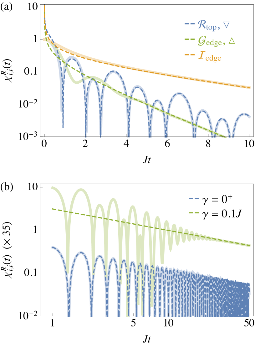
Figure 7: Retarded response function. (a) Generic behavior within various phases, specifically in $\mathcal{R}_{\mathrm{top}}$ at $\mu_{1}=-J$ and $\gamma=0.2J$, in $\mathcal{G}_{\mathrm{edge}}$ at $\mu_{1}=-1.5J$ and $\gamma=0.4J$, and in $\mathcal{I}_{\mathrm{edge}}$ at $\mu_{1}=-0.5J$ and $\gamma=1.5J$. The parameters for $\mathcal{R}_{\mathrm{top}}$ and $\mathcal{G}_{\mathrm{edge}}$ are marked with, respectively, an inverted blue triangle and a green triangle in Fig. 2. Thin dashed lines show the asymptotic late-time behavior given in Eqs. (41) and (44), and thick solid lines are exact numerical results. (b) Critical relaxation at $\mu=-2J$. For better visibility, the response function for $\gamma=0.1J$ is multiplied by $35$.

While the dynamics of the response function for $\mu=0$ is completely analogous to that of a single damped harmonic oscillator, the many-body character of the response function is restored when the chemical potential takes nonzero values and, consequently, the bands $\lambda_{\pm,k}$ in Eq. (IV) are dispersive. For this case, the response function cannot be calculated exactly. However, its asymptotic late-time behavior, which is of main interest with regard to dynamical criticality, can still be obtained analytically as described in Appendix E.

The behavior of the retarded response function in the phase $\mathcal{R}_{\mathrm{top}}$ is illustrated in Fig. 7(a). In both phases with a real line gap, $\mathcal{R}_{\mathrm{top}}$ and $\mathcal{R}_{\mathrm{tr}}$, the late-time asymptotic form of the response function reads

$$\chi^{R}_{i,i}(t)\sim\frac{\mathrm{e}^{-\Gamma_{R}t}}{\sqrt{2\pi Jt}}\left(A_{+}\cos(\omega_{+}t+\phi_{+}+\pi/4)\right.\\ \left.+A_{-}\sin(\omega_{-}t+\phi_{-}+\pi/4)\right).$$ (41)

That is, the response function is a superposition of two oscillatory contributions with frequencies $\omega_{\pm}$, and damps out exponentially with a decay rate $\Gamma_{R}=2\gamma$. It is worth stressing that the response function exhibits oscillations and zero crossings in both the topological and the trivial phase. The amplitudes, phases, and frequencies of the oscillatory components with $\sigma=\pm$ are given by

$$\begin{gathered}A_{\sigma}=\frac{\left\lvert 2J+\sigma\mu\right\rvert}{\sqrt{2\omega_{\sigma}\left\lvert\mu\right\rvert}},\quad\phi_{\sigma}=\arg\!\left(\frac{\omega_{\sigma}-\mathrm{i}2\gamma}{\left\lvert 2J+\sigma\mu\right\rvert}\right),\\ \omega_{\sigma}=\sqrt{\left(2J+\sigma\mu\right)^{2}-4\gamma^{2}}.\end{gathered}$$ (42)

When $\gamma$ is increased towards the critical value $\gamma_{\mathrm{c}}=J+\mu/2$ which marks the boundary between the phases $\mathcal{R}_{\mathrm{top}}$ and $\mathcal{G}_{\mathrm{edge}}$ for $\mu<0$, the amplitude $A_{+}$ diverges and, therefore, the asymptotic behavior of the response function is dominated by the contribution which oscillates at the frequency $\omega_{+}$. This frequency vanishes at the phase boundary. In particular, for $\gamma=\gamma_{\mathrm{c}}-\delta\gamma$, we obtain $\omega_{+}\sim 2\sqrt{\left(2J+\mu\right)\delta\gamma}$. Thus, upon approaching $\delta\gamma=0$, the oscillation period $2\pi/\omega_{+}\sim\delta\gamma^{-\epsilon}$ diverges with the same exponent $\epsilon=1/2$ as $t_{1}$. For $\mu>0$, the roles of $\sigma=+$ and $\sigma=-$ are interchanged: $A_{-}$ diverges and $\omega_{-}$ vanishes at the phase boundary, while $A_{+}$ and $\omega_{+}$ remain finite.

For both a flat and a dispersive spectrum of the Liouvillian, which lead to Eqs. (40) and (41) for the response function, respectively, the period of oscillations of the response function diverges when the real line gap closes. However, there are notable differences between Eqs. (40) and (41). First, the latter equation does not reduce to Eq. (40) in the limit $\mu\to 0$, which shows that this limit does not commute with the late-time limit $t\to\infty$ in which Eq. (41) is valid. The continuum of modes, which contribute to the response function in a many-body system, results in additional structure of Eq. (41) in comparison to Eq. (40). In particular, the exponential decay is augmented by an algebraic factor $1/\sqrt{t}$ in Eq. (41). Further, while the entire spectrum becomes purely damped with $\mathop{\mathrm{Re}}(\lambda)=0$ for critical damping with $\gamma=J$ at $\mu=0$, for a generic point on the boundary between a real-line gapped phase and a gapless phase, the behavior of the many-body response function is determined by a continuum of modes $\lambda$. Even within the gapless phases there are modes for which $\mathop{\mathrm{Re}}(\lambda)\neq 0$, as shown in Fig. 3(b). These modes give subleading oscillatory contributions with frequency $\mathop{\mathrm{Re}}(\lambda)$ to the response function, while the leading asymptotic late-time behavior is determined by modes with the smallest values of the damping rate $-\mathop{\mathrm{Im}}(\lambda)$. For these modes, the oscillation frequency vanishes, $\mathop{\mathrm{Re}}(\lambda)=0$. The damped oscillatory contribution is clearly visible for the line in Fig. 7(a) which corresponds to $\mathcal{G}_{\mathrm{edge}}$. Due to these differences between Eqs. (40) and (41), we refer to the divergence of the period of oscillations of the response function at finite values of the chemical potential as many-body critical damping. Exactly on the boundary between $\mathcal{R}_{\mathrm{top}}$ and $\mathcal{G}_{\mathrm{edge}}$, the retarded response function behaves as

$$\chi^{R}_{i,i}(t)\sim\frac{\gamma_{\mathrm{c}}}{\sqrt{2J\left\lvert\mu\right\rvert}}\mathrm{e}^{-2\Gamma_{R}t},$$ (43)

where $\gamma_{\mathrm{c}}=J-\left\lvert\mu\right\rvert/2$ and $\Gamma_{R}=2\gamma_{c}$.

The late-time form of the response function in the gapless phase $\mathcal{G}_{\mathrm{edge}}$ is shown in Fig. 7(a). In fact, the leading asymptotic behavior of the response function is the same in two gapless phases $\mathcal{G}_{\mathrm{edge}}$ and $\mathcal{G}_{\mathrm{tr}}$ as well as the imaginary-line gapped phases $\mathcal{I}_{\mathrm{edge}}$ and $\mathcal{I}_{\mathrm{tr}}$. This is because the modes with the smallest decay rates $-\mathop{\mathrm{Im}}(\lambda)$, which determine the late-time asymptotics, have the same behavior $\mathop{\mathrm{Re}}(\lambda)=0$ and $-\mathop{\mathrm{Im}}(\lambda)\sim a+bk^{2}$ for $k\to 0$ with positive real coefficients $a$ and $b$, as illustrated in Figs. 3(b) and 3(c) for $\mathcal{G}_{\mathrm{edge}}$ and $\mathcal{I}_{\mathrm{edge}}$, respectively. As a result, we find

$$\chi^{R}_{i,i}(t)\sim\frac{\mathrm{e}^{-\Gamma_{R}t}}{4\sqrt{\pi Jt\left\lvert\mu\right\rvert}}\left(\frac{2\gamma}{\sqrt{2\gamma-\Gamma_{R}}}+\sqrt{2\gamma-\Gamma_{R}}\right).$$ (44)

Here, the decay rate is given by

$$\Gamma_{R}=2\gamma-\sqrt{4\gamma^{2}-\left(2J-\left\lvert\mu\right\rvert\right)^{2}}.$$ (45)

As can be seen in Fig. 7(a), the behavior of the response function in the gapless phase $\mathcal{G}_{\mathrm{edge}}$ and the imaginary-line gapped phase $\mathcal{I}_{\mathrm{edge}}$ differs by the presence of subleading oscillatory contributions in the former case.

The above results for the late-time asymptotics of the retarded response function allow us to justify our finding in Sec. V.1.1, that the numerically determined decay rate $\Gamma_{\mathrm{max}}$ of the largest entanglement eigenvalue $\xi_{\mathrm{max}}$ agrees with the analytical expression given in Eq. (25). Indeed, by combining Eqs. (41), (43), and (44), we see that decay rate $\Gamma_{R}$ of the retarded response function is related to $\Gamma_{\mathrm{max}}$ by

$$\Gamma_{\mathrm{max}}=2\Gamma_{R}.$$ (46)

The factor of two can be explained by comparing Eqs. (22) and (94) for the covariance matrix and the retarded response function, respectively. In the former equation, the matrix $X$ appears twice in the exponent, and, therefore, the covariance matrix decays twice as fast. The maximum of $\Gamma_{R}$ and $\Gamma_{\mathrm{max}}$ at $\gamma=\gamma_{\mathrm{c}}$ is again in agreement with the physics of a damped harmonic oscillator, which decays fastest for critical damping.

Upon approaching the critical lines at $\mu=\pm 2J$ which separate the gapless phases $\mathcal{G}_{\mathrm{edge}}$ and $\mathcal{G}_{\mathrm{tr}}$, the decay rate (45) vanishes as $\Gamma_{R}\sim\delta\mu^{2}/(4\gamma)$, where we set $\mu=\mu_{\mathrm{c}}-\delta\mu$ for $\mu_{\mathrm{c}}=2J$ and $\delta\mu>0$. That is, the response function exhibits critical slowing down with a divergent relaxation time scale. Exactly on the critical lines at $\mu=\pm 2J$, the response function decays as a power law,

$$\chi^{R}_{i,i}(t)\sim\frac{1}{2J}\sqrt{\frac{\gamma}{\pi t}}.$$ (47)

As is illustrated in Fig. 7(b), subleading oscillations of the response function damp out for $t\to\infty$.

In stark contrast to the critical relaxation of the response function at the boundary between the gapless phases $\mathcal{G}_{\mathrm{edge}}$ and $\mathcal{G}_{\mathrm{tr}}$, according to Eq. (43), the response function exhibits exponential decay on the line of many-body critical damping, i.e., the phase boundary between $\mathcal{R}_{\mathrm{top}}$ and $\mathcal{G}_{\mathrm{edge}}$. This difference of exponential vs. power-law decay can be traced backed to the different types of gap closings at the boundaries between $\mathcal{R}_{\mathrm{top}}$ and $\mathcal{G}_{\mathrm{edge}}$, and $\mathcal{G}_{\mathrm{edge}}$ and $\mathcal{G}_{\mathrm{tr}}$, respectively. In the latter case, the point gap at $\lambda=0$ closes, and critical relaxation results from the existence of a continuum of modes which includes $\lambda=0$: Technically, scaling behavior is due to the integral in Eq. (95) over a continuum of modes, which develops a singularity when the continuum includes zero. In contrast, although the real line gap closes at the phase boundary between $\mathcal{R}_{\mathrm{top}}$ and $\mathcal{G}_{\mathrm{edge}}$, the point gap at $\lambda=0$ remains intact.

Finally, we note that the retarded response function can be calculated exactly at $\mu=\pm 2J$ and in the limit $\gamma=0^{+}$ when we assume that the system reaches the trivial infinite-temperature steady state even for vanishingly small dissipation. We find

$$\chi^{R}_{i,i}(t)=\frac{1}{2}\theta(t)J_{0}(4Jt),$$ (48)

where $J_{n}(z)$ is a Bessel function of the first kind with late-time asymptotic behavior

$$\chi^{R}_{i,i}(t)\sim\sin(4Jt+\pi/4)/\sqrt{2\pi Jt}.$$ (49)

Thus, for $\gamma=0^{+}$, oscillations of the response function persist indefinitely, as can be seen in Fig. 7(b).

VI Systems with non-Hermitian jump operators

So far, we have mainly focused on a special case of the driven-dissipative Kitaev chain: For $\gamma_{\mathrm{l}}=\gamma_{\mathrm{g}}$, the jump operators (4) are Hermitian, and the steady state of the time evolution described by the master equation (2) is a trivial infinite-temperature state. We showed that for Hermitian jump operators, non-Hermitian topology of the Liouvillian $\hat{\mathcal{L}}$ is revealed through entanglement spectrum crossings in quench dynamics. Now we proceed to discuss the general case of non-Hermitian jump operators with $\gamma_{\mathrm{l}}\neq\gamma_{\mathrm{g}}$, where the interplay of unitary and dissipative dynamics results in a nontrivial steady state. As we explain in the following, in this general case, the presence or absence of entanglement spectrum crossings is determined not only by the topology of $\hat{\mathcal{L}}$, but also by properties of the initial and steady states.

In particular, as discussed in Sec. V.1.2, each zero crossing in the single-particle entanglement spectrum is accompanied by a reversal of the fermion parity of the entanglement ground state. Therefore, if the initial and steady states have opposite parities, an entanglement spectrum crossing must occur even if the topology of $\hat{\mathcal{L}}$ is trivial. However, as we show below, the connection between non-Hermitian topology of $\hat{\mathcal{L}}$ and entanglement spectrum crossings can be restored by means of Hermitianization of the jump operators Lieu et al. (2020).

VI.1 Fermion parity and Pfaffian in the initial and steady states

For Hermitian jump operators, which lead to a trivial steady state $\rho_{\mathrm{ss}}=\rho_{\infty}=\mathbbm{1}/D$, also the reduced density matrix is trivial, $\rho_{A,\mathrm{ss}}={\mathop{\mathrm{tr}}}_{A^{\mathrm{c}}}(\rho_{\mathrm{ss}})=\mathbbm{1}_{A}/D_{A}$ with $D_{A}=2^{N/2}$. The corresponding many-body entanglement spectrum is flat, and states with even and odd fermion parity are degenerate. Consequently, the parity of the entanglement ground state is undetermined. Further, the covariance matrix of the steady state vanishes identically. Thus, also the sign of the steady-state Pfaffian $\mathrm{Pf}_{\mathrm{ss}}$ is undetermined.

In contrast, for non-Hermitian jump operators with $\gamma_{\mathrm{l}}\neq\gamma_{\mathrm{g}}$, the entanglement spectrum of the steady state is nondegenerate, and the corresponding entanglement ground state has definite fermion parity $p_{A,\mathrm{ss}}$. The sign of the steady-state Pfaffian is given by

$$\mathop{\mathrm{sgn}}(\mathrm{Pf}_{\mathrm{ss}})=p_{A,\mathrm{ss}}=\left(\mathop{\mathrm{sgn}}(\delta)\right)^{N/2}$$ (50)

with $\delta=\gamma_{\mathrm{l}}-\gamma_{\mathrm{g}}$. As we show in Appendix F, this relation holds for $J=\Delta>0$, and arbitrary postquench values of the chemical potential $\mu_{1}$. Notably, if $\delta<0$, Eq. (50) exhibits an even-odd half-system-size effect for $\mathop{\mathrm{sgn}}(\mathrm{Pf}_{\mathrm{ss}})$. Here, as in Sec. V, we restrict our discussion to systems with an even number of lattice sites, $N\in 2\mathbb{N}$, such that $N/2\in\mathbb{N}$ is an integer.

Equation (50) should be compared with the corresponding relation for the initial state of the quench protocol, i.e., the ground state of the Hamiltonian (1) of the Kitaev chain. In the trivial phase with $\left\lvert\mu_{0}\right\rvert>2J$, we find

$$\mathop{\mathrm{sgn}}(\mathrm{Pf}_{0})=p_{A,0}=\left(-\mathop{\mathrm{sgn}}(\mu_{0})\right)^{N/2}.$$ (51)

For values of $\mu_{0}$, $\delta$, and $N/2$ that lead to disagreements between the right-hand sides of Eqs. (50) and (51), there must be a reversal of the sign of the Pfaffian in the course of the time evolution, and, consequently, also a crossing in the entanglement spectrum. This conclusion does not rely on the topology of the Liouvillian, and can even be in conflict with expectations based on the latter. In particular, for $\delta<0$ and $\mu_{0}<0$, Eqs. (50) and (51) imply that an entanglement spectrum crossing must occur if $N/2$ is odd. By contrast, we should expect no crossing if $N/2$ is even. This even-odd half-system-size effect cannot be captured by the non-Hermitian winding number $W$, which is defined for the bands of an infinite bulk system.

We proceed to demonstrate the occurrence of the even-odd effect explicitly in the time evolution of entanglement spectra, and we then show how the discrepancy between the entanglement spectrum crossings and the topology of the Liouvillian can be resolved through Hermitianization of the jump operators.

VI.2 Quench dynamics with non-Hermitian and Hermitianized jump operators

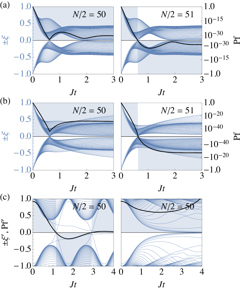
Figure 8: Quench dynamics for non-Hermitian jump operators. (a) Quench to the topological phase $\mathcal{R}_{\mathrm{top}}$ with $\gamma_{\mathrm{l}}=0.3J$ and $\gamma_{\mathrm{g}}=0.7J$ such that $\delta=\gamma_{\mathrm{l}}-\gamma_{\mathrm{g}}=-0.4J$, and $\mu_{1}=0$. Left panel: For $N/2=50$, $\mathop{\mathrm{sgn}}(\mathrm{Pf}_{0})=\mathop{\mathrm{sgn}}(\mathrm{Pf}_{\mathrm{ss}})=1$, and the Pfaffian stays positive at all times. Right panel: For $N/2=51$, $\mathop{\mathrm{sgn}}(\mathrm{Pf}_{\mathrm{ss}})=-1$, and the Pfaffian exhibits a single zero crossing. (b) Quench to the trivial phase $\mathcal{G}_{\mathrm{edge}}$ for $\mu_{1}=-1.5J$ and the same values of $\gamma_{\mathrm{l}}$ and $\gamma_{\mathrm{g}}$ as in (a). Again, a single entanglement spectrum crossing occurs when $N/2$ is odd. (c) The connection between entanglement spectrum crossings and topology is restored for the deformed Liouvillian with Hermitianized jump operators and a trivial steady state. The left and right panels correspond to quenches with the parameters of (a) and (b), respectively. We show the rescaled entanglement spectrum $\xi^{\prime}=\xi\mathrm{e}^{2\left(\gamma_{\mathrm{l}}+\gamma_{\mathrm{g}}\right)t}$ and Pfaffian $\mathrm{Pf}^{\prime}=\mathop{\mathrm{Pf}}\mathrm{e}^{2\left(\gamma_{\mathrm{l}}+\gamma_{\mathrm{g}}\right)Nt}$ for $N/2=50$. The corresponding plots for $N/2=51$ look essentially the same.

The impact of the even-odd effect of the Pfaffians of the initial and steady states on the time evolution of the entanglement spectrum is illustrated in Fig. 8. In particular, Fig. 8(a) shows the evolution of the single-particle entanglement spectrum for a quench to the topological phase $\mathcal{R}_{\mathrm{top}}$ with $\gamma_{\mathrm{l}}=0.3J$, $\gamma_{\mathrm{g}}=0.7J$, and $\mu_{1}=0$. For these parameter values, the bulk spectrum (IV) of the Liouvillian becomes flat, and we might expect periodically recurring entanglement spectrum crossings. However, as shown in the figure, there is no entanglement spectrum zero crossing for $N/2=50$, and only a single crossing for $N/2=51$. These findings are in agreement with our expectations based on Eqs. (50) and (51).

In the course of the time evolution, the Pfaffian drops rapidly to very small values. Indeed, as discussed in Appendix F.2, the steady-state Pfaffian $\mathrm{Pf}_{\mathrm{ss}}$ is exponentially small in $N$. However, there we also show that the parity $p_{A,\mathrm{ss}}$, and, therefore, the sign of $\mathrm{Pf}_{\mathrm{ss}}$ are well-defined for arbitrarily large systems.

Quenches to the gapless trivial phase $\mathcal{G}_{\mathrm{edge}}$ with the same values of $\gamma_{\mathrm{l}}$ and $\gamma_{\mathrm{g}}$ as above and $\mu_{1}=-1.5J$ are shown in Fig. 8(b). Again, there is no entanglement spectrum zero crossing for $N/2=50$, and only a single zero crossing for $N/2=51$.

The presence or absence of entanglement spectrum crossings can be reconciled with the topological properties of the Liouvillian $\hat{\mathcal{L}}$ through Hermitianization of the jump operators, i.e., by continuously deforming the jump operators to make them Hermitian as described in Ref. Lieu et al. (2020). Hermitianization of the jump operators corresponds to a transformation of the matrices $X$ and $Y$ that determine the Liouvillian through Eq. (8), in the course of which $X=\mathrm{const.}$, while $Y\to 0$. That is to say, the spectral gap and the symmetries of the Liouvillian are preserved, whereas the steady state becomes trivial with $\mathrm{Pf}_{\mathrm{ss}}=0$. Consequently, for a master equation with Hermitianized jump operators, the even-odd half-system size effect is resolved.

In particular, for the quenches shown in Figs. 8(a) and 8(b), the time evolution of the entanglement spectrum with Hermitianized jump operators is shown in, respectively, the left and right panel of Fig. 8(c). Both for $N/2=50$ as shown in the figure and for $N/2=51$, entanglement spectrum crossings occur only when the non-Hermitian winding number of the postquench Liouvillian takes the value $W=1$.

Hermitianization of the jump operators allows us to explore the entire topological phase diagram for $\gamma_{\mathrm{l}}\neq\gamma_{\mathrm{g}}$ in terms of entanglement spectrum zero crossings. This is illustrated in Fig. 9. For the value $\mu_{1}=0$ shown in the figure, the real-line gapped phase $\mathcal{R}_{\mathrm{top}}$ borders the phase $\mathcal{I}_{\mathrm{edge}}$ with an imaginary line gap. The time scale $t_{1}$, at which the first entanglement spectrum crossing occurs, diverges at the boundary of the topological phase $\mathcal{R}_{\mathrm{top}}$. In particular, as shown in the inset of Fig. 9, $t_{1}$ exhibits power-law behavior, $t_{1}\sim\delta\gamma^{-\epsilon}$. For the value of the exponent, we find $\epsilon=1/2$ in agreement with our results for Hermitian jump operators.

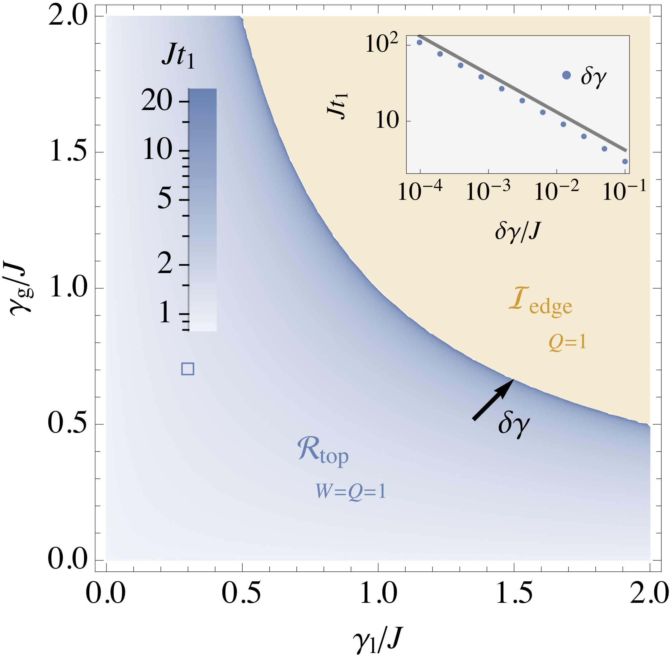
Figure 9: Dynamical topological phase diagram for Hermitianized jump operators and with $\mu_{1}=0$. Labels of the phases and the color scale are the same as in Fig. 2. Inset: As for the case of Hermitian jump operators, $t_{1}$ diverges at the boundary of $\mathcal{R}_{\mathrm{top}}$ with a critical exponent of $\epsilon=1/2$. The data shown corresponds to approaching the phase boundary along the black arrow labeled by $\delta\gamma$ in the main panel, i.e., $\gamma_{\mathrm{l}}=\gamma_{\mathrm{l},\mathrm{c}}-\delta\gamma$ and $\gamma_{\mathrm{g}}=\gamma_{\mathrm{g},\mathrm{c}}-\delta\gamma$, where $\gamma_{\mathrm{l},\mathrm{c}}=1.5J$ and, according to Eq. (17), $\gamma_{\mathrm{g},\mathrm{c}}=J^{2}/\gamma_{\mathrm{l},\mathrm{c}}$. For comparison, the gray solid line shows a square-root singularity. The system size is $N=100$ both in the inset and the main panel.

VII Conclusions and Outlook

Our work establishes the entanglement spectrum as a tool to study non-Hermitian dynamical topology of driven and open quantum many-body systems. We circumvent the problem that complex spectra do not allow to define ground states Herviou et al. (2019) by considering the time evolution of entanglement spectra after a quench.

We show that for systems with Hermitian or Hermitianized jump operators, the presence of entanglement spectrum crossings reflects nontrivial topology of individual complex bands of the Liouvillian. The topology of individual bands is characterized by the non-Hermitian winding number $W$. In contrast, as discussed in Ref. Lieu (2018), the presence of edge modes is tied to the global Berry phase $Q$, which pertains to the full spectrum, and is well-defined also in gapless phases. The existence of two distinct topological transitions, at which, respectively, the value of the non-Hermitian winding number $W$ and the global Berry phase $Q$ changes, is unique to non-Hermitian systems. Indeed, as shown in the dynamical topological phase diagram in Fig. 2, the corresponding phase boundaries between $\mathcal{R}_{\mathrm{top}}$ and $\mathcal{G}_{\mathrm{edge}}$ as well as $\mathcal{G}_{\mathrm{edge}}$ and $\mathcal{G}_{\mathrm{tr}}$, coincide in the Hermitian limit where the rate of dissipation $\gamma$ vanishes.

The characterization of non-Hermitian dynamical topology through the entanglement spectrum opens up interesting directions for future research. While we focus here on a driven and dissipative version of the Kitaev chain, which belongs to the non-Hermitian symmetry class $\mathrm{BDI}^{\dagger}$ Kawabata et al. (2019), our approach can be applied directly to Liouvillian generalizations Lieu et al. (2020) of the Altland-Zirnbauer symmetry classes that accommodate nontrivial $(1+1)$-dimensional dynamical topology Gong and Ueda (2018).

Apart from different one-dimensional and noninteracting models, as well as other symmetry classes, a promising prospect is to generalize the entanglement spectrum bulk-edge correspondence to quench dynamics of driven-dissipative systems in higher spatial dimensions, and of interacting open quantum many-body systems. Analogous generalizations were obtained for isolated Hermitian systems in Refs. Chang (2018); Gong and Ueda (2018). For noninteracting Hermitian and non-Hermitian systems, the existence of a band structure is sufficient to define topological invariants, even without referring to a particular state. By contrast, for interacting Hermitian systems, a well-defined ground state commonly forms the basis of any discussion of topology Chiu et al. (2016). This raises the following questions: How can the topology of the complex spectra of quartic Liouvillians, which describe interacting open quantum many-body systems, be classified? Do sharp dynamical topological transitions exist also for such systems? Our approach based on the entanglement spectrum provides a way to address, in particular, the latter question. For example, we expect that also for a generalization of an interacting Kitaev chain Fidkowski (2010), which includes Markovian drive and dissipation, the time evolution of the many-body entanglement spectrum carries signatures of non-Hermitian dynamical topology of the quartic Liouvillian.

A substantial part of our work is concerned with a detailed investigation of dynamical criticality at the two distinct topological phase transitions which are related to the non-Hermitian winding number $W$ and the global Berry phase $Q$. We find strikingly different behavior: While the transition that is described by $Q$ exhibits conventional critical relaxation, we observe the phenomenon of many-body critical damping at the boundaries of the topological phase $\mathcal{R}_{\mathrm{top}}$ with $W=1$.

Our analysis of dynamical criticality, and, in particular, of many-body critical damping, opens up new avenues for future research, which bear relevance beyond the field of non-Hermitian topology. An obvious question is whether it is possible to identify different universality classes of many-body critical damping. To address this question, it will be interesting to study, e.g., a driven and open Kitaev chain with long-range hopping and pairing Vodola et al. (2014); Alecce and Dell’Anna (2017); Maity et al. (2020), or to explore whether the dynamical critical exponent for entanglement spectrum crossings is renormalized due to interactions.

The focus of the present work is to explore theoretically signatures of non-Hermitian topology in the time evolution of the entanglement spectrum. A natural next step is to devise experimental implementations of the physics discussed in our work. The required building blocks are available in synthetic quantum systems: First, realizations of Kitaev chain have been proposed in systems of cold atoms Jiang et al. (2011); Nascimbène (2013); Hu and Baranov (2015); Kraus et al. (2013). Alternatively, the transverse field Ising model, to which the Kitaev chain is mapped through the Jordan-Wigner transformation Fendley (2012), can be implemented in quantum simulators of many-body spin systems such as trapped atomic ions Monroe et al. (2019), Rydberg atom arrays Browaeys and Lahaye (2020), or superconducting qubits Viehmann et al. (2013); Barends et al. (2016). Further, Markovian dissipation, which is described by a quantum master equation with Hermitian jump operators, can be induced by subjecting the system to classical noise. This approach has been used, e.g., to implement local dephasing of individual spins in a recent experiment with trapped ions Maier et al. (2019). Finally, the measurement of entanglement spectra in various experimental platforms has been developed in Refs. Pichler et al. (2016); Dalmonte et al. (2018); Kokail et al. (2020).

These developments open up the prospect to experimentally explore non-Hermitian topology of driven and open quantum many-body systems, and thus go fundamentally beyond the paradigm of classical non-Hermitian wave physics. A comprehensive understanding of the robust signatures of non-Hermitian topology in quantum many-body systems is central for this endeavour. Our work, which identifies entanglement spectrum crossings as such a signature, represents an important step in this direction.

Appendix A Driven-dissipative Kitaev chain with quasilocal Hermitian jump operators

Our key findings, which are summarized in Sec. II, are derived for a driven-dissipative Kitaev chain with strictly local jump operators. In the following, we provide evidence for the general validity of our conclusions by presenting results for the quasilocal Hermitian jump operators given in Eq. (5).

The dynamical topological phase diagram of the driven-dissipative Kitaev chain with quasilocal jump operators is shown in Fig. 10. A comparison with Fig. 2 reveals two important qualitative differences: First, for quasilocal jump operators, there is a direct phase boundary between the real-line gapped topological $\mathcal{R}_{\mathrm{top}}$ and trivial $\mathcal{R}_{\mathrm{tr}}$ phases, even at finite values of the dissipation rate $\kappa$. Second, the model with quasilocal jump operators does not exhibit phases with an imaginary line gap. We proceed with a concise summary of the key properties of the driven-dissipative Kitaev chain with quasilocal jump operators.

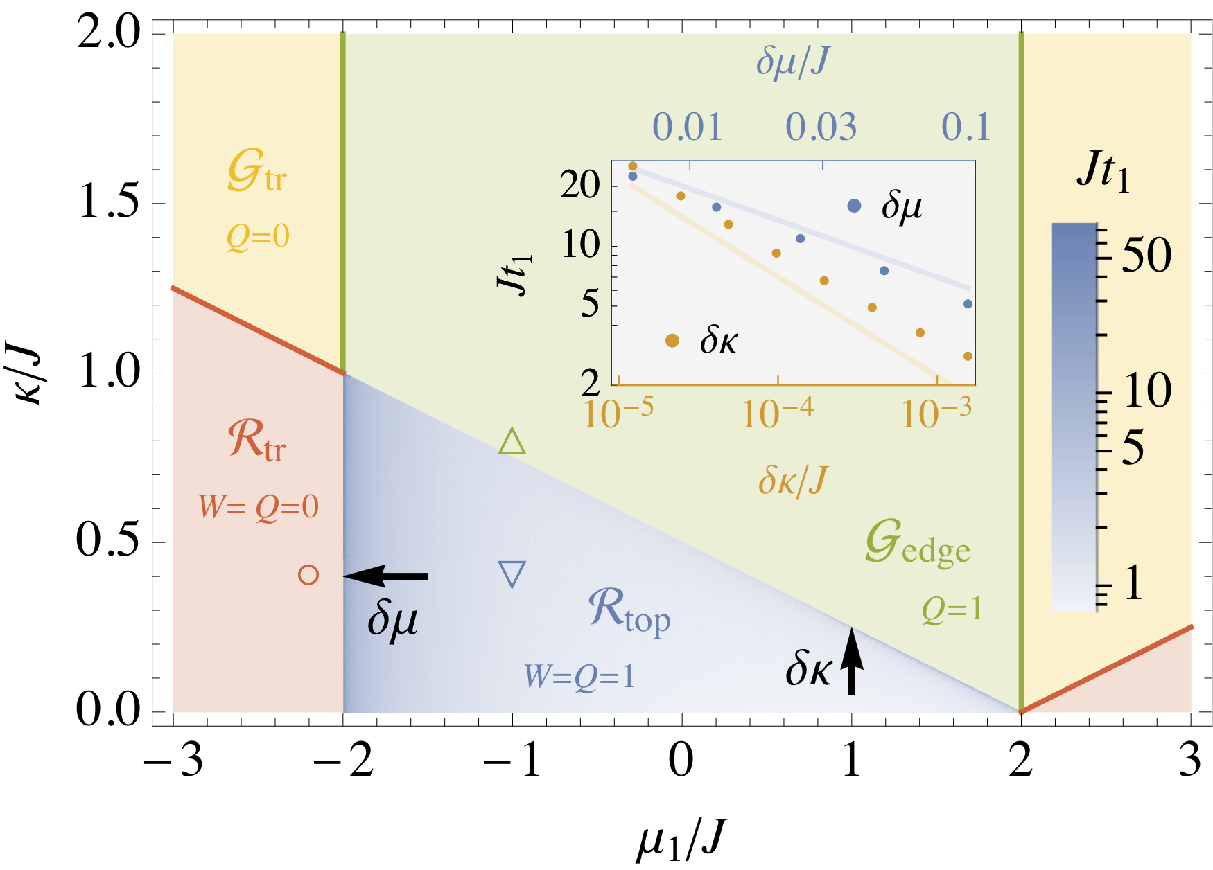
Figure 10: Dynamical topological phase diagram of a driven-dissipative Kitaev chain with quasilocal jump operators. The designations of different phases and the logarithmic color scale in $\mathcal{R}_{\mathrm{top}}$ are the same as in Fig. 2. The values of $t_{1}$ are obtained for a quench with a half-flattened Liouvillian as explained in Sec. A.1. Light blue and orange lines in the inset correspond to square-root singularities and have different slopes due to different scales for $\delta\mu$ and $\delta\kappa$. The system size is $N=100$ both in the inset and the main panel.

A.1 Non-Hermitian band theory

The bulk spectrum of the Liouvillian is determined by the eigenvalues of the matrix

$$z_{k}=-\mathrm{i}2\kappa\left(1-\cos(k)\right)\mathbbm{1}+\mathbf{z}_{k}\cdot\boldsymbol{\sigma},$$ (52)

where

$$\mathbf{z}_{k}=\left(2\Delta\sin(k),2J\cos(k)+\mu,-\mathrm{i}2\kappa\left(1-\cos(k)\right)\right).$$ (53)

We obtain two complex bands which are given by

$$\lambda_{\pm,k}=-\mathrm{i}2\kappa\left(1-\cos(k)\right)\pm\left[4\Delta^{2}\sin(k)^{2}\vphantom{\left(1-\cos(k)\right)^{2}}\right.\\ \left.+\left(2J\cos(k)+\mu\right)^{2}-4\kappa^{2}\left(1-\cos(k)\right)^{2}\right]^{1/2}.$$ (54)

For $4\kappa<\left\lvert 2J-\mu\right\rvert$, the expression in brackets is positive for all values of the quasimomentum $k$, and the spectrum exhibits a real line gap. Spectra in the two phases $\mathcal{R}_{\mathrm{top}}$ and $\mathcal{R}_{\mathrm{tr}}$ with a real line gap are shown in Figs. 11(a) and 11(b), respectively.

As illustrated in Fig. 11(c), the spectrum is gapless for $4\kappa>\left\lvert 2J-\mu\right\rvert$. In the phase diagram in Fig. 10, the two gapless phases are designated by $\mathcal{G}_{\mathrm{edge}}$ and $\mathcal{G}_{\mathrm{tr}}$. Unlike the case of local jump operators, the spectrum remains gapless even for high values of $\kappa$, and the present model does not have phases with an imaginary line gap.

The symmetries stated in Eq. (19) remain intact for quasilocal jump operators, and the system still belongs to the class $\mathrm{BDI}^{\dagger}$. We omit details of the straightforward calculation of the non-Hermitian winding number $W$ for brevity. This calculation yields $W=1$ in $\mathcal{R}_{\mathrm{top}}$ and $W=0$ in $\mathcal{R}_{\mathrm{tr}}$. Further, the global Berry phase is given by $Q=1$ for $\left\lvert\mu\right\rvert<2J$ and $Q=0$ for $\left\lvert\mu\right\rvert>2J$. Edge modes, which occur in $\mathcal{R}_{\mathrm{top}}$ and $\mathcal{G}_{\mathrm{edge}}$ where $Q=1$, are indicated by black diamond symbols in Fig. 11. At the critical lines $\mu=\pm 2J$, where the edge modes disappear, the point gap of the bands $\lambda_{\pm,k}$ at $\lambda=0$ closes.

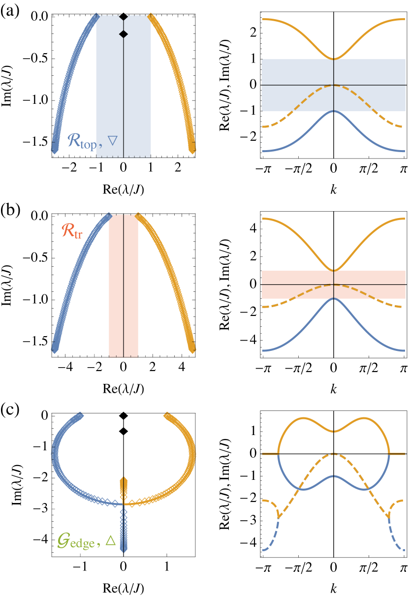
Figure 11: Liouvillian spectra of a driven-dissipative Kitaev chain with quasilocal jump operators and for $J=\Delta$. The notation and symbols are the same as those in Fig. 3. The spectrum exhibits a real line gap in (a) the topological phase $\mathcal{R}_{\mathrm{top}}$, shown here for $\kappa=0.4J$ and $\mu=-J$, and (b) the trivial phase $\mathcal{R}_{\mathrm{tr}}$, shown for $\mu=-3J$ and $\kappa=0.4J$. (c) Gapless spectrum in $\mathcal{G}_{\mathrm{edge}}$ at $\mu=-J$ and $\kappa=0.8J$.

A notable difference between the spectra shown in Figs. 3 and 11 is the wide dispersion of imaginary parts $\mathop{\mathrm{Im}}(\lambda_{\pm,k})$ which occurs in the case of quasilocal jump operators. The coexistence of modes with widely disparate decay rates hampers the numerical analysis of the present model. In particular, the time evolution of entanglement spectra, which we discuss in the next section, is hard to resolve for values of $\kappa$ close to $\kappa=J$ within the topological phase $\mathcal{R}_{\mathrm{tr}}$ in Fig. 10. To mitigate this problem, we consider dynamics generated by a band-flattened Liouvillian. Band-flattening can be achieved through a continuous deformation of the original Liouvillian, and, therefore, does not affect its topology Kawabata et al. (2019).

Our starting point is the third-quantized form of the Liouvillian $\hat{\mathcal{L}}$ given in Eq. (8). As explained in Sec. III.2, the spectrum of $\mathrm{i}\hat{\mathcal{L}}$ is determined by the matrix $Z=-\mathrm{i}X^{{\mathchoice{\raisebox{0.0pt}{$\displaystyle\intercal$}}{\raisebox{0.0pt}{$\textstyle\intercal$}}{\raisebox{0.0pt}{$\scriptstyle\intercal$}}{\raisebox{0.0pt}{$\scriptscriptstyle\intercal$}}}}$. To resolve the problem of disparate decay rates, it is sufficient to consider a half-flatttened Liouvillian, which we obtain by replacing $Z=V\Lambda V^{-1}$, with $\Lambda=\mathop{\mathrm{diag}}(\lambda_{1},\dotsc,\lambda_{2N})$ a diagonal matrix, by $Z_{\mathrm{hf}}=V\mathop{\mathrm{Re}}(\Lambda)V^{-1}$, i.e., by removing the decay rates $-\mathop{\mathrm{Im}}(\Lambda)$ by hand. We note that the spectrum becomes completely flat if $Z$ is replaced by $Z_{\mathrm{fl}}=JV\mathop{\mathrm{sgn}}(\mathop{\mathrm{Re}}(\Lambda))V^{-1}$, where the prefactor $J$ is introduced as an arbitrary overall energy scale. However, $Z_{\mathrm{fl}}$ is well-defined only if there are no eigenvalues of $Z$ with vanishing real part. The time-evolved entanglement spectra which we discuss below, as well as the data for $t_{1}$ shown in Fig. 10, are obtained with a half-flattened Liouvillian.

A.2 time evolution of entanglement spectra

Entanglement spectrum crossings reveal non-Hermitian topology of the Liouvillian also for a driven-dissipative Kitaev chain with quasilocal Hermitian jump operators. This is illustrated in Figs. 12(a) and 12(b) for quenches to $\mathcal{R}_{\mathrm{top}}$ and $\mathcal{R}_{\mathrm{tr}}$, respectively. For time evolution with a half-flattened Liouvillian, the entangement spectrum does not show significant decay, and most entanglement eigenvalues remain close to $\pm 1$.

A quantitative analysis of the time $t_{1}$ of the first entanglement spectrum zero crossing within the entire phase $\mathcal{R}_{\mathrm{top}}$ is shown in Fig. 10. The logarithmic color scale indicates that $t_{1}$ diverges at the boundaries of $\mathcal{R}_{\mathrm{top}}$. This is illustrated further in the inset, which shows the increase of $t_{1}$ upon approaching the phase boundary along the black arrows in the main panel, i.e., for $\delta\mu=\mu_{1}+2J\to 0$ with $\kappa=0.4J$, and for $\mu_{1}=J$ with $\delta\kappa=J/4-\kappa\to 0$. The numerical data is consistent with a square-root singularity, and, therefore, corroborates the universality of the value $\epsilon=1/2$ of the dynamical critical exponent for entanglement spectrum crossings.

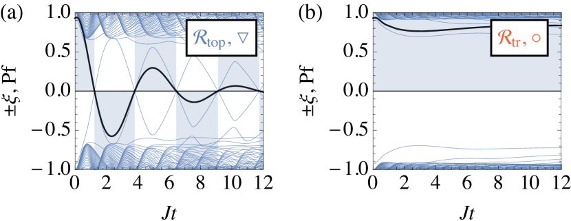
Figure 12: Time evolution of entanglement spectra. The dynamics is generated by a half-flattened Liouvillian as explained in the main text. (a) Zero crossings in the entangement spectrum occur for a quench to $\mathcal{R}_{\mathrm{top}}$ with $W=1$ at $\mu_{1}=-J$ and $\kappa=0.4J$. (b) The entanglement spectrum remains gapped for a quench to $\mathcal{R}_{\mathrm{tr}}$ with $W=0$ at $\mu_{1}=-2.2J$ and $\kappa=0.4J$.

Appendix B Covariance matrix in the ground state

To find the covariance matrix of the ground state of the Kitaev chain, we start from the Majorana representation of the Hamiltonian given in Eq. (7). The matrix $A$ in this equation is real and antisymmetric. Therefore, there exists a real special orthogonal matrix $O$ which brings $A$ to the following canonical block-diagonal form:

$$OAO^{{\mathchoice{\raisebox{0.0pt}{$\displaystyle\intercal$}}{\raisebox{0.0pt}{$\textstyle\intercal$}}{\raisebox{0.0pt}{$\scriptstyle\intercal$}}{\raisebox{0.0pt}{$\scriptscriptstyle\intercal$}}}}=\bigoplus\limits_{i=1}^{N}\begin{pmatrix}0&-\epsilon_{i}\\ \epsilon_{i}&0\end{pmatrix},$$ (55)

where $\epsilon_{i}\geq 0$. The matrix $O$ can be found by employing the algorithm described in Ref. Wimmer (2012). Then, the covariance matrix of the ground state is given by Kraus et al. (2009)

$$\Gamma_{A,0}=O^{{\mathchoice{\raisebox{0.0pt}{$\displaystyle\intercal$}}{\raisebox{0.0pt}{$\textstyle\intercal$}}{\raisebox{0.0pt}{$\scriptstyle\intercal$}}{\raisebox{0.0pt}{$\scriptscriptstyle\intercal$}}}}\left(\bigoplus\limits_{i=1}^{N}\mathrm{i}\sigma_{y}\right)O.$$ (56)

Appendix C Exactly solvable quench dynamics

Here we derive the exact solution in Eq. (28) for the time evolution of the reduced density matrix. We obtain this exact solution for a specific choice of pre- and postequench parameters as detailed in the following.

C.1 Initial state

We assume that the system is initialized in the ground state $\lvert\psi_{0}\rangle$ of the Hamiltonian of the Kitaev chain for $J=\Delta>0$ and $\mu_{0}\to-\infty$, which is the vacuum of Dirac fermions $c_{i}$, i.e., $\lvert\psi_{0}\rangle=\lvert\Omega\rangle$ with $c_{i}\lvert\Omega\rangle=0$ for all $i=1,\dotsc,N$. The corresponding density matrix is

$$\rho_{0}=\lvert\psi_{0}\rangle\langle\psi_{0}\rvert=\lvert\Omega\rangle\langle\Omega\rvert=\prod_{i=1}^{N}\rho_{i,0},\quad\rho_{i,0}=P^{0}_{i}.$$ (57)

Here and below, we use the following notation for projectors on states for which the lattice site $i$ is empty and occupied, respectively:

$$P^{0}_{i}=1-n_{i}=\lvert 0\rangle_{i}\langle 0\rvert,\qquad P^{1}_{i}=n_{i}=\lvert 1\rangle_{i}\langle 1\rvert,$$ (58)

where the site occupation number operator is $n_{i}=c_{i}^{\dagger}c_{i}$.

C.2 Postquench Liouvillian

For the choice of postquench parameters $J=\Delta$, $\mu_{1}=0$, and $\gamma_{\mathrm{l}}=\gamma_{\mathrm{g}}=\gamma$, the third-quantized Liouvillian (8) takes the form

$$\hat{\mathcal{L}}=-4\gamma\hat{n}_{1}-2\sum_{i=1}^{N-1}\left(\hat{c}_{2i}^{\dagger},\hat{c}_{2i+1}^{\dagger}\right)\begin{pmatrix}0&J\\ -J&2\gamma\end{pmatrix}\begin{pmatrix}\hat{c}_{2i}\\ \hat{c}_{2i+1}\end{pmatrix},$$ (59)

where the site occupation number superoperator is defined as $\hat{n}_{i}=\hat{c}_{i}^{\dagger}\hat{c}_{i}$. Left and right edge modes are created by the superoperators $\hat{c}_{L}^{\dagger}=\hat{c}_{1}^{\dagger}$ and $\hat{c}_{R}^{\dagger}=\hat{c}_{2N}^{\dagger}$, respectively. The corresponding eigenvalues of $\mathrm{i}\hat{\mathcal{L}}$ are $\lambda_{L}=-\mathrm{i}4\gamma$ and $\lambda_{R}=0$. Since $\mathop{\mathrm{Re}}(\lambda_{L})=\mathop{\mathrm{Re}}(\lambda_{R})=0$, the dynamics of these modes is purely dissipative. In contrast, the dynamics of bulk modes has both oscillatory and dissipative components. The bulk spectrum is flat and consist of two values $\lambda_{\pm}$, which are determined by the eigenvalues of the matrix in the second term in Eq. (59), and are given in Eq. (26).

To separate the dissipative and oscillatory contributions to the dynamics of the bulk, we decompose the Liouvillian as $\hat{\mathcal{L}}=\hat{\mathcal{L}}_{0}+\hat{\mathcal{L}}_{1}$, where

$$\hat{\mathcal{L}}_{0}=\sum_{i=1}^{N}\hat{\mathcal{L}}_{0,i},\qquad\hat{\mathcal{L}}_{1}=\sum_{i=1}^{N-1}\hat{\mathcal{L}}_{1,i}$$ (60)

with

$$\hat{\mathcal{L}}_{0,i}=\begin{cases}-2\gamma\left(2\hat{n}_{1}+\hat{n}_{2}\right)&\text{for }i=1,\\ -2\gamma\left(\hat{n}_{2i-1}+\hat{n}_{2i}\right)&\text{for }i=2,\dotsc N-1,\\ -2\gamma\hat{n}_{2N-1}&\text{for }i=N,\end{cases}$$ (61)

and

$$\hat{\mathcal{L}}_{1,i}=2\left[\gamma\left(\hat{n}_{2i}-\hat{n}_{2i+1}\right)-J\left(\hat{c}_{2i}^{\dagger}\hat{c}_{2i+1}-\hat{c}_{2i+1}^{\dagger}\hat{c}_{2i}\right)\right].$$ (62)

With the aid of anticommutation relation of superoperators stated in Sec. III.2, it is straightforward to check that $\hat{\mathcal{L}}_{0}$ and $\hat{\mathcal{L}}_{1}$ commute. Therefore, the time evolution superoperator factorizes as

$$\mathrm{e}^{\hat{\mathcal{L}}t}=\mathrm{e}^{\hat{\mathcal{L}}_{1}t}\mathrm{e}^{\hat{\mathcal{L}}_{0}t}.$$ (63)

We proceed to analyze first the dissipative, and then the oscillatory component of the dynamics.

C.3 Dissipative dynamics

The Liouvillian $\hat{\mathcal{L}}_{0}$ in Eq. (60) is a sum of commuting terms $\hat{\mathcal{L}}_{0,i}$, which describe the evolution of fermions on lattice site $i$. Further, since the initial density matrix (57) factorizes in real space, we obtain

$$\mathrm{e}^{\hat{\mathcal{L}}_{0}t}\rho_{0}=\prod_{i=1}^{N}\mathrm{e}^{\hat{\mathcal{L}}_{0,i}t}\rho_{0,i},$$ (64)

and, therefore, we can consider each site $i$ independently.

We begin by collecting a few useful relations: First, by expanding the exponential in a power series and using that $\hat{n}_{i}^{2}=\hat{n}_{i}$, we find

$$\mathrm{e}^{-2\gamma t\hat{n}_{i}}=\hat{1}-\left(1-\mathrm{e}^{-2\gamma t}\right)\hat{n}_{i}.$$ (65)

Next, from the Majorana representation of the site occupation number operator, $n_{i}=\frac{1}{2}\left(1-\mathrm{i}w_{2i-1}w_{2i}\right)$, it follows that

$$\hat{n}_{2i-1}n_{i}=\hat{n}_{2i}n_{i}=-\frac{\mathrm{i}}{2}w_{2i-1}w_{2i}=n_{i}-\frac{1}{2}.$$ (66)

With these relations, it is straightforward to show that

$$\mathrm{e}^{-2\gamma t\hat{n}_{2i-1}}P^{0}_{i}=\mathrm{e}^{-2\gamma t\hat{n}_{2i}}P^{0}_{i}\\ =\frac{1}{2}\left[\left(1+\mathrm{e}^{-2\gamma t}\right)P^{0}_{i}+\left(1-\mathrm{e}^{-2\gamma t}\right)P^{1}_{i}\right],$$ (67)

and

$$\mathrm{e}^{-2\gamma t\hat{n}_{2i-1}}P^{1}_{i}=\mathrm{e}^{-2\gamma t\hat{n}_{2i}}P^{1}_{i}\\ =\frac{1}{2}\left[\left(1-\mathrm{e}^{-2\gamma t}\right)P^{0}_{i}+\left(1+\mathrm{e}^{-2\gamma t}\right)P^{1}_{i}\right],$$ (68)

where the projectors $P^{0}_{i}$ and $P^{1}_{i}$ are defined in Eq. (58). Thus, the evolution (64) of the density matrix under the local Liouvillians $\hat{\mathcal{L}}_{0,i}$ is given by

$$\mathrm{e}^{\hat{\mathcal{L}}_{0,i}t}\rho_{0,i}=\frac{1}{2}\sum_{n=0}^{1}\left[1+\left(-1\right)^{n}\mathrm{e}^{-2\gamma_{i}t}\right]P^{n}_{i},$$ (69)

where $\gamma_{1}=3\gamma$, $\gamma_{N}=\gamma$, and $\gamma_{i}=2\gamma$ for $i=2,\dotsc,N-1$.

C.4 Oscillatory dynamics

We next consider the oscillatory component $\hat{\mathcal{L}}_{1}$. The local contributions $\hat{\mathcal{L}}_{1,i}$ in Eq. (62) commute, and we can again consider the evolution which is generated by each of them separately. Since $\hat{\mathcal{L}}_{1,i}$ commutes with the sum of number superoperators $\hat{N}_{i}=\hat{n}_{2i}+\hat{n}_{2i+1}$, it can be decomposed into three contributions that correspond to the eigenspaces of $\hat{N}_{i}$,

$$\hat{\mathcal{L}}_{1,i}=\lvert 1\rrangle\hat{\mathcal{L}}_{1,i}^{(0)}\llangle 1\rvert\\ +\left(\lvert w_{2i}\rrangle,\lvert w_{2i+1}\rrangle\right)\hat{\mathcal{L}}_{1,i}^{(1)}\begin{pmatrix}\llangle w_{2i}\rvert\\ \llangle w_{2i+1}\rvert\end{pmatrix}\\ +\lvert w_{2i}w_{2i+1}\rrangle\hat{\mathcal{L}}_{1,i}^{(2)}\llangle w_{2i}w_{2i+1}\rvert,$$ (70)

where

$$\begin{split}\hat{\mathcal{L}}_{1,i}^{(0)}&=\llangle 1|\hat{\mathcal{L}}_{1,i}|1\rrangle=0,\\ \hat{\mathcal{L}}_{1,i}^{(2)}&=\llangle w_{2i}w_{2i+1}|\hat{\mathcal{L}}_{1,i}|w_{2i}w_{2i+1}\rrangle=0,\end{split}$$ (71)

and

$$\begin{split}\hat{\mathcal{L}}_{1,i}^{(1)}&=\begin{pmatrix}\llangle w_{2i}|\hat{\mathcal{L}}_{1,i}|w_{2i}\rrangle&\llangle w_{2i}|\hat{\mathcal{L}}_{1,i}|w_{2i+1}\rrangle\\ \llangle w_{2i+1}|\hat{\mathcal{L}}_{1,i}|w_{2i}\rrangle&\llangle w_{2i+1}|\hat{\mathcal{L}}_{1,i}|w_{2i+1}\rrangle\end{pmatrix},\\ &=2\begin{pmatrix}\gamma&-J\\ J&-\gamma\end{pmatrix}=2\left(\gamma\sigma_{z}-\mathrm{i}J\sigma_{y}\right).\end{split}$$ (72)

To calculate $\mathrm{e}^{\hat{\mathcal{L}}_{1,i}^{(1)}t}$, we use the following relation which holds for $\mathbf{a}\in\mathbb{C}^{3}$ and where $\boldsymbol{\sigma}=\left(\sigma_{x},\sigma_{y},\sigma_{z}\right)$:

$$\mathrm{e}^{-\mathrm{i}\mathbf{a}\cdot\boldsymbol{\sigma}t}=\cos(at)\mathbbm{1}-\mathrm{i}\sin(at)\frac{\mathbf{a}\cdot\boldsymbol{\sigma}}{a},\quad a^{2}=\sum_{i=1}^{3}a_{i}^{2}.$$ (73)

For $\mathbf{a}=2\left(0,J,\mathrm{i}\gamma\right)$, we find $a=\pi/T$ where $T$ is given in Eq. (27), and thus

$$\mathrm{e}^{\hat{\mathcal{L}}_{1,i}^{(1)}t}=\cos(\pi t/T)\mathbbm{1}+\frac{2T}{\pi}\sin(\pi t/T)\left(\gamma\sigma_{z}-\mathrm{i}J\sigma_{y}\right).$$ (74)

In particular, for $t=mT$, where $m\in\mathbb{N}_{0}$ is a nonnegative integer, we obtain

$$\mathrm{e}^{\hat{\mathcal{L}}_{1,i}^{(1)}mT}=\cos(\pi m)\mathbbm{1}=\left(-1\right)^{m}\mathbbm{1},$$ (75)

and, therefore,

$$\mathrm{e}^{\hat{\mathcal{L}}_{1,i}mT}=\lvert 1\rrangle\llangle 1\rvert+\lvert w_{2i}w_{2i+1}\rrangle\llangle w_{2i}w_{2i+1}\rvert\\ +\left(-1\right)^{m}\left(\lvert w_{2i}\rrangle\llangle w_{2i}\rvert+\lvert w_{2i+1}\rrangle\llangle w_{2i+1}\rvert\right),$$ (76)

which can also be written in the compact form

$$\mathrm{e}^{\hat{\mathcal{L}}_{1,i}mT}=\mathrm{e}^{\mathrm{i}\pi m\left(\hat{n}_{2i}+\hat{n}_{2i+1}\right)}.$$ (77)

The oscillatory evolution of the entire chain is thus given by the product

$$\mathrm{e}^{\hat{\mathcal{L}}_{1}mT}=\prod_{i=1}^{N-1}\mathrm{e}^{\hat{\mathcal{L}}_{1,i}mT}=\mathrm{e}^{\mathrm{i}\pi m\left(\hat{n}_{1}+\hat{n}_{2N}\right)}\hat{P}^{m},$$ (78)

where $\hat{P}$ is the parity superoperator which is defined as

$$\hat{P}=\mathrm{e}^{\mathrm{i}\pi\sum_{i=1}^{2N}\hat{n}_{i}}=\prod_{i=1}^{2N}\left(1-2\hat{n}_{i}\right).$$ (79)

Finally, we note that the evolution superoperator can be simplified for even and odd values of $m$, respectively:

$$\mathrm{e}^{\hat{\mathcal{L}}_{1}mT}=\begin{cases}\hat{1}&\text{for $m$ even,}\\ \left(\hat{1}-2\hat{n}_{1}\right)\left(\hat{1}-2\hat{n}_{2N}\right)\hat{P}&\text{for $m$ odd.}\end{cases}$$ (80)

C.5 Time evolution of the density matrix

We now combine Eq. (69) with Eq. (80) to find the time-evolved density matrix $\rho(mT)$. According to Eq. (80), at times $mT$, not only the dissipative evolution under $\hat{\mathcal{L}}_{0}$, but also the oscillatory dynamics generated by $\hat{\mathcal{L}}_{1}$ factorizes in real space:

$$\rho(mT)=\mathrm{e}^{\hat{\mathcal{L}}_{1}mT}\mathrm{e}^{\hat{\mathcal{L}}_{0}mT}\rho_{0}=\prod_{i=1}^{N}\rho_{i}(mT).$$ (81)

To determine $\rho_{i}(mT)$ explicitly, we have to apply superoperators $\hat{1}-2\hat{n}_{i}$, which occur in Eqs. (79) and (80), to the projectors $P^{n}_{i}$ in Eq. (69). This can be done with the aid of the relations

$$\left(\hat{1}-2\hat{n}_{i}\right)P^{0}_{i}=P^{1}_{i},\quad\left(\hat{1}-2\hat{n}_{i}\right)P^{1}_{i}=P^{0}_{i},$$ (82)

which follow from Eqs. (58) and (66), and which immediately lead to

$$\left(1-2\hat{n}_{2i-1}\right)\left(1-2\hat{n}_{2i}\right)P^{n}_{i}=P^{n}_{i}$$ (83)

for $n=0,1$. We thus find

$$\rho_{i}(mT)=\frac{1}{2}\sum_{n=0}^{1}\left[1+\left(-1\right)^{m_{i}+n}\mathrm{e}^{-2\gamma_{i}mT}\right]P^{n}_{i},$$ (84)

where $m_{i}=m$ for $i=1,N$, and $m_{i}=0$ for $i=2,\dotsc,N-1$. Each of the reduced density matrices for a single lattice site $i$ has trace one, $\mathop{\mathrm{tr}}_{i}(\rho_{i}(mT))=1$. Therefore, the reduced density matrix for the left half of the chain is simply given by the product

$$\rho_{A}(mT)=\prod_{i=1}^{N/2}\rho_{i}(mT)\\ =\sum_{\mathbf{n}}\frac{1}{2}\left[1+\left(-1\right)^{m+n_{1}}\xi_{1,m}\right]P_{1}^{n_{1}}\\ \times\prod_{i=2}^{N/2}\frac{1}{2}\left[1+\left(-1\right)^{n_{i}}\xi_{2,m}\right]P_{i}^{n_{i}},$$ (85)

where the sum in the second equality is over all combinations $\mathbf{n}=\left(n_{1},\dotsc,n_{N/2}\right)$ of site occupation numbers, and $\xi_{m,1}$ and $\xi_{m,2}$ are given in Eq. (29). Finally, we obtain Eq. (28) by noting that $P^{\mathbf{n}}=\lvert\mathbf{n}\rangle_{A}\langle\mathbf{n}\rvert=\prod_{i=1}^{N/2}P_{i}^{n_{i}}$, and by replacing the sum over site occupation numbers $\mathbf{n}$ in Eq. (85) by a sum over entanglement occupation numbers $\mathbf{e}=\left(e_{1},\dotsc,e_{N/2}\right)$ with $e_{1}=(n_{1}+m)\bmod 2$ and $e_{i}=n_{i}$ for $i=2,\dotsc,N/2$. Inverting the relation between $\mathbf{e}$ and $\mathbf{n}$ leads to Eq. (30).

Appendix D Conservation of parity of entanglement eigenstates

In the following, we show that the fermion parity of any individual entanglement eigenstate is conserved. To this end, we note first that the fermion parity operator $P=\mathrm{e}^{\mathrm{i}\pi\sum_{i=1}^{2N}n_{i}}$ is related to the parity superoperator (79) via $\hat{P}\rho=P\rho P$. This can be checked by expanding the density matrix $\rho$ in the basis of products of Majorana operators specified in Sec. III.2. The relation between $\hat{P}$ and $P$ implies that the density matrix $\rho=\lvert\psi\rangle\langle\psi\rvert$ for any pure state $\lvert\psi\rangle$ which has definite positive or negative parity has positive superparity. In particular, this applies to the ground state of the Hamiltonian of the Kitaev chain (1), which is the initial state of the quench protocol we consider in the present work.

The superparity of the initial state is conserved under time evolution with a quadratic Liouvillian Prosen (2008). This follows from the equality $[\hat{P},\hat{\mathcal{L}}]=0$, which further implies that the density matrix can be diagonalized in a basis of states with definite fermion parity at all times,

$$\rho=\sum_{n}c_{n}\lvert\psi_{n}\rangle\langle\psi_{n}\rvert,\qquad P\lvert\psi_{n}\rangle=p_{n}\lvert\psi_{n}\rangle,$$ (86)

with $p_{n}=\pm 1$. Consequently, also the reduced density matrix $\rho_{A}={\mathop{\mathrm{tr}}}_{A^{\mathrm{c}}}(\rho)$ for a subsystem $A$ can be diagonalized in a basis of eigenstates of the corresponding fermion parity operator $P_{A}$, which is defined in Eq. (32),

$$\rho_{A}=\sum_{l}\Xi_{l}\lvert\phi_{l}\rangle\langle\phi_{l}\rvert,\qquad P_{A}\lvert\phi_{l}\rangle=p_{A,l}\lvert\phi_{l}\rangle.$$ (87)

This can be seen as follows: A single state $\lvert\psi_{n}\rangle$, which occurs in Eq. (86), can be written as

$$\lvert\psi_{n}\rangle=\sum_{\alpha,\beta}c_{\alpha\beta}\lvert e^{A}_{\alpha},e^{A^{\mathrm{c}}}_{\beta}\rangle+\sum_{\alpha,\beta}d_{\alpha\beta}\lvert o^{A}_{\alpha},o^{A^{\mathrm{c}}}_{\beta}\rangle,$$ (88)

where the states $\lvert e^{A,A^{\mathrm{c}}}_{\alpha}\rangle$ and $\lvert o^{A,A^{\mathrm{c}}}_{\alpha}\rangle$ form a basis of states which contain, respectively, an even and odd number of fermions in $A$ and its complement $A^{\mathrm{c}}$, and for concreteness we assume that $\lvert\psi_{n}\rangle$ has even parity. Upon taking the trace over $A^{\mathrm{c}}$, we find

$$\rho_{A}^{n}={\mathop{\mathrm{tr}}}_{A^{\mathrm{c}}}(\lvert\psi_{n}\rangle\langle\psi_{n}\rvert)=\sum_{\alpha,\alpha^{\prime},\beta}c_{\alpha\beta}c_{\alpha^{\prime}\beta}^{*}\lvert e^{A}_{\alpha}\rangle\langle e^{A}_{\alpha^{\prime}}\rvert\\ +\sum_{\alpha,\alpha^{\prime},\beta}d_{\alpha\beta}d_{\alpha^{\prime}\beta}^{*}\lvert o^{A}_{\alpha}\rangle\langle o^{A}_{\alpha^{\prime}}\rvert.$$ (89)

That is, the reduced density matrix $\rho_{A}^{n}$ is composed of two disconnected blocks corresponding to states with even and odd particle number, respectively. It follows that $P_{A}\rho_{A}^{n}P_{A}=\rho_{A}^{n}$. An analogous argument applies to states $\lvert\psi_{n}\rangle$ with odd parity and, therefore, to all states in the sum in Eq. (86). This proves Eq. (87), according to which entanglement eigenstates have definite parity at all times.

Appendix E Retarded response function

Here we provide details on the calculation of the retarded response function defined in Eq. (37). Two-time averages can be obtained with the aid of the quantum regression theorem Gardiner and Zoller (2014), which yields for $t>0$

$$\begin{split}\langle w_{i}(t)w_{j}\rangle&=\mathop{\mathrm{tr}}(w_{i}\mathrm{e}^{\mathcal{L}t}(w_{j}\rho_{\mathrm{ss}})),\\ \langle w_{j}w_{i}(t)\rangle&=\mathop{\mathrm{tr}}(w_{i}\mathrm{e}^{\mathcal{L}t}(\rho_{\mathrm{ss}}w_{j})),\\ \end{split}$$ (90)

and, therefore,

$$\chi^{R}_{i,j}(t)=\frac{1}{2}\theta(t)\mathop{\mathrm{tr}}(w_{i}\mathrm{e}^{\mathcal{L}t}\{w_{j},\rho_{\mathrm{ss}}\})=\theta(t)\mathop{\mathrm{tr}}(w_{i}\mathrm{e}^{\mathcal{L}t}w_{j}).$$ (91)

In the second equality, we specified the trivial steady state $\rho_{\mathrm{ss}}=\mathbbm{1}/D$. A closed equation of motion can be derived for the response matrix, which collects all possible combinations of odd and even position indices,

$$R_{i,j}(t)=\begin{pmatrix}\chi^{R}_{2i-1,2j-1}(t)&\chi^{R}_{2i-1,2j}(t)\\ \chi^{R}_{2i,2j-1}(t)&\chi^{R}_{2i,2j}(t)\end{pmatrix}.$$ (92)

The equation of motion, which results from taking the derivative of Eq. (91), takes a particularly simple form in momentum space:

$$\frac{\mathrm{d}R_{k}}{\mathrm{d}t}=\delta(t)\mathbbm{1}+R_{k}\widetilde{x}_{-k},$$ (93)

where $R_{k}(t)=\sum_{j\in\mathbb{Z}}\mathrm{e}^{-\mathrm{i}kj}R_{i+j,i}(t)$, $\widetilde{x}_{k}=x_{k}-4\mathop{\mathrm{tr}}(M)$, and $x_{k}=\mathrm{i}z_{k}^{{\mathchoice{\raisebox{0.0pt}{$\displaystyle\intercal$}}{\raisebox{0.0pt}{$\textstyle\intercal$}}{\raisebox{0.0pt}{$\scriptstyle\intercal$}}{\raisebox{0.0pt}{$\scriptscriptstyle\intercal$}}}}$. For the local dissipative model, $z_{k}$ is given in Eq. (13), and $\mathop{\mathrm{tr}}(M)=\gamma$. The solution to Eq. (93) reads

$$R_{k}(t)=\theta(t)\mathrm{e}^{\widetilde{x}_{-k}t},$$ (94)

which yields the equal-position retarded response function as

$$R_{i,i}(t)=\int_{-\pi}^{\pi}\frac{\mathrm{d}k}{2\pi}\,R_{k}(t).$$ (95)

To obtain the late-time asymptotics of the retarded response function quoted in Sec. V.2 and illustrated in Fig. 7, we evaluate the integral over quasimomenta using standard techniques of asymptotic analysis Bender and Orszag (1999). The numerical results shown in Fig. 7 result from a direct numerical integration of Eq. (95).

Appendix F Even-odd half-system-size effect

In this appendix, we derive Eqs. (50) and (51), which describe the even-odd half-system-size effect of the fermion parity of the entanglement ground state, and the sign of the Pfaffian.

F.1 Even-odd effect of the fermion parity

Before we confirm Eqs. (50) and (51) numerically for arbitrary values of $\mu_{0}$ and $\delta$, it is instructive to consider certain limiting cases, in which the fermion parities $p_{A,0}$ and $p_{A,\mathrm{ss}}$ of the entanglement ground states of the initial and steady states, respectively, can be determined in a straightforward manner.

For $J=\Delta>0$ and $\mu_{0}\to-\infty$, the ground state of the Hamiltonian (1) of the Kitaev chain is the vacuum state $\lvert\Omega\rangle$, which obeys $c_{i}\lvert\Omega\rangle=0$ for all $i=1,\dotsc,N$; for $\mu_{0}\to\infty$, the ground state is the completely filled state $\prod_{i=1}^{N}c_{i}^{\dagger}\lvert\Omega\rangle$. In the lattice-site occupation representation introduced in Sec. V.1.2, the corresponding entanglement ground states are $\lvert\mathbf{0}\rangle_{A}$ and $\lvert\mathbf{1}\rangle_{A}$, where $\mathbf{1}=\left(1,\dotsc,1\right)$. For the vacuum state, the fermion parity $p_{A,0}$ of the entanglement ground state is even, $p_{A,0}=1$. In contrast, for the completely filled state, the parity depends on the size of the system as $p_{A,0}=\left(-1\right)^{N/2}$, i.e., the parity is even or odd if half of the system size is even or odd, respectively. As in the main text, we consider systems with an even number of lattice sites, $N\in 2\mathbb{N}$, such that $N/2\in\mathbb{N}$ is an integer.

With regard to the steady state, we consider the following limits of the value of $\delta=\gamma_{\mathrm{l}}-\gamma_{\mathrm{g}}$: For $\delta\to\infty$, the steady state is the vacuum state with $p_{A,\mathrm{ss}}=1$; for $\delta\to-\infty$, the steady state is the completely filled state with $p_{A,\mathrm{ss}}=\left(-1\right)^{N/2}$.

If the difference of parities is finite, $p_{A,0}-p_{A,\mathrm{ss}}\neq 0$, in the course of the quench dynamics, there has to be at least one reversal of the parity of the entanglement ground state, and, concomitantly, a zero crossing in the single-particle entanglement spectrum. Our findings for $p_{A,0}$ and $p_{A,\mathrm{ss}}$, and the resulting expectations for the presence or absence of entanglement spectrum crossings, are summarized in Table 1.

	vacuum	filled
	$\delta\to\infty$	$\delta\to-\infty$
	$p_{A,\mathrm{ss}}=1$	$p_{A,\mathrm{ss}}=\left(-1\right)^{N/2}$
vacuum		crossings are
$\mu_{0}\to-\infty$	no crossing	present/absent if
$p_{A,0}=1$		$N/2$ is odd/even
filled	crossings are
$\mu_{0}\to\infty$	present/absent if	no crossing
$p_{A,0}=\left(-1\right)^{N/2}$	$N/2$ is odd/even

Table 1: Even-odd half-system-size effect for the parity in the initial and steady state, and, consequently, for the presence or absence of entanglement spectrum crossings. The initial and steady states are the vacuum state or the completely filled state, $\lvert\Omega\rangle$ or $\prod_{i=1}^{N}c_{i}^{\dagger}\lvert\Omega\rangle$, respectively, for the given limiting values of $\mu_{0}$ and $\delta$.

F.2 Pfaffian in the initial and steady state

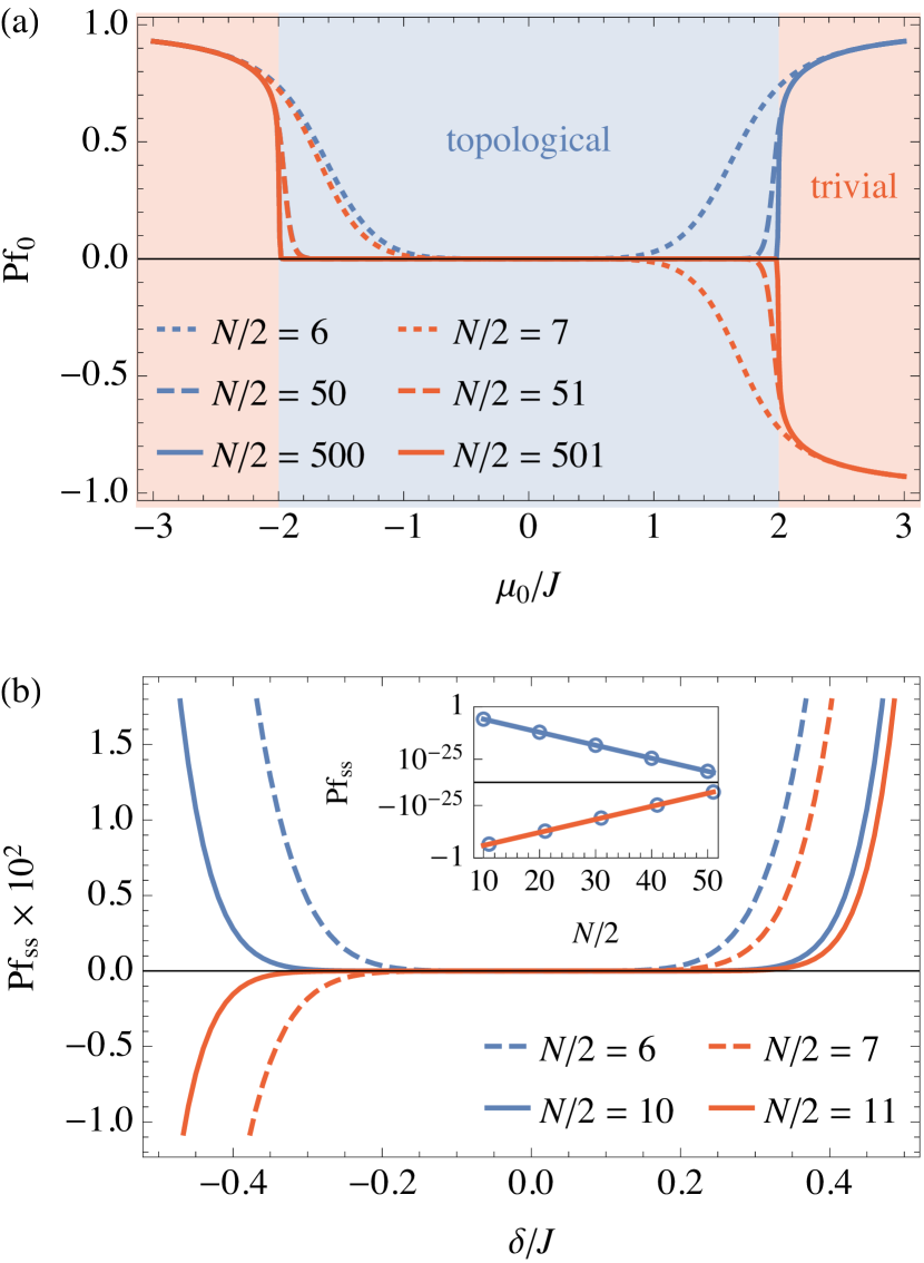
Figure 13: Even-odd effect of the Pfaffian $\mathrm{Pf}$ and the parity $p_{A}$ of the entanglement ground state. (a) The Pfaffian in the ground state $\mathrm{Pf}_{0}$ vanishes in the topological phase for $\left\lvert\mu_{0}\right\rvert<2J$ in the thermodynamic limit, and the parity is undetermined. In the trivial phase, $\mathop{\mathrm{sgn}}(\mathrm{Pf}_{0})$ obeys Eq. (51). (b) The sign of the Pfaffian and the parity in the steady state with $\gamma_{\mathrm{l}}+\gamma_{\mathrm{g}}=J$ are given by Eq. (50). Inset: $\mathrm{Pf}_{\mathrm{ss}}$ vanishes exponentially for $N\to\infty$ as indicated by the linear behavior on the logarithmic scale. For the value $\delta=-0.4J$ chosen here, $\mathop{\mathrm{sgn}}(\mathrm{Pf}_{\mathrm{ss}})$ alternates for even and odd half-system sizes $N/2=10,11,20,21,\dotsc,50,51$ shown in the figure. In (b), the chemical potential is $\mu_{1}=0$. In both panels, $J=\Delta>0$.

We proceed to confirm numerically and for generic values of pre- and postquench parameters, that the sign of the Pfaffian $\mathrm{Pf}$ (24) of the reduced covariance matrix of the initial and steady states exhibits the same half-system-size dependence as the fermion parity $p_{A}$ of the corresponding entanglement ground state. Indeed, in all cases we consider, we find $\mathop{\mathrm{sgn}}(\mathrm{Pf})=p_{A}$. The parity can be calculated as described in Appendix G.

The even-odd half-system-size effect for the Pfaffian is illustrated in Fig. 13. In particular, Fig. 13(a) shows the Pfaffian of the reduced covariance matrix of the ground state of the Kitaev chain with open boundary conditions as a function of the chemical potential $\mu_{0}$. For increasing system size, the Pfaffian $\mathrm{Pf}_{0}$ develops a sharp drop to zero at the critical values $\mu_{0}=\pm 2J$. In the topological phase of the Kitaev chain, for $\left\lvert\mu_{0}\right\rvert<2J$, the Pfaffian $\mathrm{Pf}_{0}$ is equal to zero, which reflects the presence of a zero-energy edge mode at the entanglement cut. Indeed, since the square of the Pfaffian equals the determinant of the reduced covariance matrix, $\mathrm{Pf}_{0}=0$ if one of the single-particle entanglement eigenvalues $\xi_{i}$ is equal to zero. In the trivial phase with $\left\lvert\mu_{0}\right\rvert>2J$, the sign of $\mathrm{Pf}_{0}$ is given by Eq. (51).

In Appendix F.1, we argued that the fermion parity of the entanglement ground state in the steady state is always positive for $\delta\to\infty$, whereas it exhibits an even-odd half-system-size effect in the limit $\delta\to-\infty$. As shown in Fig. 13(b), the Pfaffian in the steady state exhibits an analogous even-odd half-system-size effect also for finite values of the imbalance of dissipation rates $\delta=\gamma_{\mathrm{l}}-\gamma_{\mathrm{g}}$. This confirms Eq. (50) for the values $\gamma_{\mathrm{l}}+\gamma_{\mathrm{g}}=J$ and $\mu_{1}=0$, chosen in the figure. We checked that Eq. (50) holds also for nonzero values of $\mu_{1}$.

The dependence of $\mathrm{Pf}_{\mathrm{ss}}$ on the half-system size $N/2$ is illustrated further in the inset of Fig. 13(b), which shows $\mathrm{Pf}_{\mathrm{ss}}$ for $\delta=-0.4J$ and a series of half-system sizes $N/2=10,11,20,21,\dotsc,50,51$. While the linear behavior of $\mathrm{Pf}_{\mathrm{ss}}$ on the logarithmic scale clearly indicates exponential decay of the magnitude of the steady-state Pfaffian, the fermion parity of the entanglement ground state, and, therefore, the sign of the Pfaffian, is well-defined for arbitrarily large values of $N$. This follows from the fact that for $\delta\neq 0$, the single-particle entanglement spectrum retains a finite gap $\Delta\xi>0$ for $N\to\infty$, and that a finite gap implies a unique entanglement ground state with well-defined parity. In the limits $\delta\to\pm\infty$, the entanglement gap is $\Delta\xi=1$ for the vacuum and completely filled state, respectively, as follows from the explicit expressions $\Gamma_{A}^{\mathrm{vac}}=\mathrm{i}\bigoplus_{i=1}^{N/2}\sigma_{y}=-\Gamma_{A}^{\mathrm{filled}}$. For generic parameter values, we present numerical evidence for a finite entanglement gap in Fig. 14.

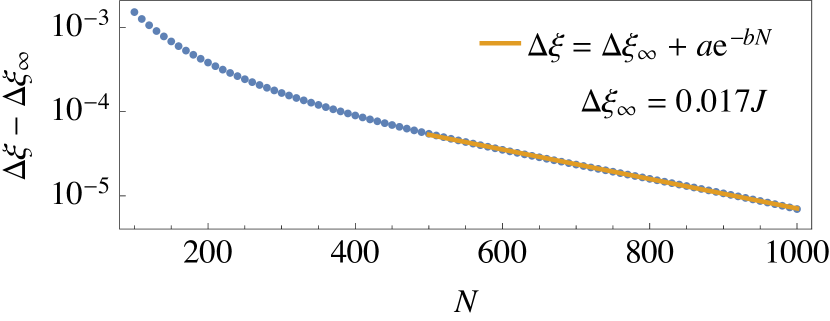
Figure 14: The gap $\Delta\xi$ of the single-particle entanglement spectrum approaches its thermodynamic value $\Delta\xi_{\infty}$ exponentially. The orange line is a fit to the numerical data shown as blue dots. Parameters are $\gamma_{\mathrm{l}}=0.3J$, $\gamma_{\mathrm{g}}=0.7J$, and $\mu_{1}=0$.

Appendix G Fermion parity of the entanglement ground state

A numerical evaluation of Eq. (22) yields the reduced covariance matrix $\Gamma_{A}$ at arbitrary times $t$. Here we describe how the parity of the corresponding entanglement ground state can be determined. To this end, we use the following representation of the parity operator (32)

$$P_{A}=\mathrm{e}^{\mathrm{i}\pi\sum_{i=1}^{N/2}c_{i}^{\dagger}c_{i}}=\prod_{i=1}^{N/2}\mathrm{i}w_{2i-1}w_{2i}.$$ (96)

Our goal is to calculate the expectation value of $P_{A}$ in the entanglement ground state. Since the entanglement Hamiltonian is quadratic, all of its eigenstates are Slater determinants. Therefore, expectations values of products of fermionic operators as in Eq. (96) can be found by employing Wick’s theorem, which yields Kraus et al. (2009) $\left\langle P_{A}\right\rangle=\mathop{\mathrm{pf}}(\Gamma_{A}^{0})$, where $\Gamma_{A}^{0}$ is the covariance matrix of the entanglement ground state, i.e., the ground state of the entanglement Hamiltonian. The latter can be written as Kraus et al. (2009)

$$H_{A}=\frac{\mathrm{i}}{4}\sum_{i,j=1}^{N}w_{i}G_{i,j}w_{j},$$ (97)

where the real and antisymmetric matrix $G$ can be expressed in the form

$$G=O^{{\mathchoice{\raisebox{0.0pt}{$\displaystyle\intercal$}}{\raisebox{0.0pt}{$\textstyle\intercal$}}{\raisebox{0.0pt}{$\scriptstyle\intercal$}}{\raisebox{0.0pt}{$\scriptscriptstyle\intercal$}}}}\left(\bigoplus\limits_{i=1}^{N}\begin{pmatrix}0&-\varepsilon_{i}\\ \varepsilon_{i}&0\end{pmatrix}\right)O.$$ (98)

Here, $O$ is the real special orthogonal matrix which brings the reduced covariance matrix $\Gamma_{A}$ to its canonical block-diagonal form,

$$O\Gamma_{A}O^{{\mathchoice{\raisebox{0.0pt}{$\displaystyle\intercal$}}{\raisebox{0.0pt}{$\textstyle\intercal$}}{\raisebox{0.0pt}{$\scriptstyle\intercal$}}{\raisebox{0.0pt}{$\scriptscriptstyle\intercal$}}}}=\bigoplus\limits_{i=1}^{N}\begin{pmatrix}0&\xi_{i}\\ -\xi_{i}&0\end{pmatrix},$$ (99)

and $\varepsilon_{i}=2\mathop{\mathrm{atanh}}(\xi_{i})$. The covariance matrix $\Gamma_{A}^{0}$ of the ground state of the entanglement Hamiltonian (97) can be found as described in Appendix B for the original Hamiltonian (1), and yields the parity of the entanglement ground state as described above.

References

- Esaki et al. (2011) K. Esaki, M. Sato, K. Hasebe, and M. Kohmoto, “Edge states and topological phases in non-hermitian systems,” Phys. Rev. B 84, 205128 (2011).
- Malzard et al. (2015) S. Malzard, C. Poli, and H. Schomerus, “Topologically protected defect states in open photonic systems with non-hermitian charge-conjugation and parity-time symmetry,” Phys. Rev. Lett. 115, 200402 (2015).
- Leykam et al. (2017) D. Leykam, K. Y. Bliokh, C. Huang, Y. D. Chong, and F. Nori, “Edge modes, degeneracies, and topological numbers in non-hermitian systems,” Phys. Rev. Lett. 118, 28–30 (2017).
- Shen et al. (2018) H. Shen, B. Zhen, and L. Fu, “Topological band theory for non-hermitian hamiltonians,” Phys. Rev. Lett. 120, 146402 (2018).
- Gong et al. (2018) Z. Gong, Y. Ashida, K. Kawabata, K. Takasan, S. Higashikawa, and M. Ueda, “Topological phases of non-hermitian systems,” Phys. Rev. X 8, 31079 (2018).
- Yao and Wang (2018) S. Yao and Z. Wang, “Edge states and topological invariants of non-hermitian systems,” Phys. Rev. Lett. 121, 086803 (2018).
- Kunst et al. (2018) F. K. Kunst, E. Edvardsson, J. C. Budich, and E. J. Bergholtz, “Biorthogonal bulk-boundary correspondence in non-hermitian systems,” Phys. Rev. Lett. 121, 026808 (2018).
- Kawabata et al. (2019) K. Kawabata, K. Shiozaki, M. Ueda, and M. Sato, “Symmetry and topology in non-hermitian physics,” Phys. Rev. X 9, 041015 (2019).
- Zhou and Lee (2019) H. Zhou and J. Y. Lee, “Periodic table for topological bands with non-hermitian symmetries,” Phys. Rev. B 99, 235112 (2019).
- Liu et al. (2019) C.-H. Liu, H. Jiang, and S. Chen, “Topological classification of non-hermitian systems with reflection symmetry,” Phys. Rev. B 99, 125103 (2019).
- Yokomizo and Murakami (2019) K. Yokomizo and S. Murakami, “Non-bloch band theory of non-hermitian systems,” Phys. Rev. Lett. 123, 066404 (2019).
- Borgnia et al. (2020) D. S. Borgnia, A. J. Kruchkov, and R.-J. Slager, “Non-hermitian boundary modes and topology,” Phys. Rev. Lett. 124, 056802 (2020).
- Ashida et al. (2020) Y. Ashida, Z. Gong, and M. Ueda, “Non-hermitian physics,” arXiv:2006.01837 (2020).
- Lieu et al. (2020) S. Lieu, M. McGinley, and N. R. Cooper, “Tenfold way for quadratic lindbladians,” Phys. Rev. Lett. 124, 040401 (2020).
- Dangel et al. (2018) F. Dangel, M. Wagner, H. Cartarius, J. Main, and G. Wunner, “Topological invariants in dissipative extensions of the su-schrieffer-heeger model,” Phys. Rev. A 98, 013628 (2018).
- Lieu (2019) S. Lieu, “Non-hermitian majorana modes protect degenerate steady states,” Phys. Rev. B 100, 085110 (2019).
- Song et al. (2019) F. Song, S. Yao, and Z. Wang, “Non-hermitian skin effect and chiral damping in open quantum systems,” Phys. Rev. Lett. 123, 170401 (2019).
- Minganti et al. (2019) F. Minganti, A. Miranowicz, R. W. Chhajlany, and F. Nori, “Quantum exceptional points of non-hermitian hamiltonians and liouvillians: The effects of quantum jumps,” Phys. Rev. A 100, 062131 (2019).
- Liu et al. (2020) C.-H. Liu, K. Zhang, Z. Yang, and S. Chen, “Helical damping and dynamical critical skin effect in open quantum systems,” Phys. Rev. Res. 2, 043167 (2020).
- Okuma and Sato (2020) N. Okuma and M. Sato, “Quantum anomaly, non-Hermitian skin effects, and entanglement entropy in open systems,” arXiv:2011.08175 (2020).
- Hasan and Kane (2010) M. Z. Hasan and C. L. Kane, “Colloquium: Topological insulators,” Rev. Mod. Phys. 82, 3045–3067 (2010).
- Qi and Zhang (2011) X.-L. Qi and S.-C. Zhang, “Topological insulators and superconductors,” Rev. Mod. Phys. 83, 1057–1110 (2011).
- Chiu et al. (2016) C.-K. Chiu, J. C. Y. Teo, A. P. Schnyder, and S. Ryu, “Classification of topological quantum matter with symmetries,” Rev. Mod. Phys. 88, 035005 (2016).
- Li and Haldane (2008) H. Li and F. D. M. Haldane, “Entanglement spectrum as a generalization of entanglement entropy: Identification of topological order in non-abelian fractional quantum hall effect states,” Phys. Rev. Lett. 101, 010504 (2008).
- Pollmann et al. (2010) F. Pollmann, A. M. Turner, E. Berg, and M. Oshikawa, “Entanglement spectrum of a topological phase in one dimension,” Phys. Rev. B 81, 064439 (2010).
- Fidkowski (2010) L. Fidkowski, “Entanglement spectrum of topological insulators and superconductors,” Phys. Rev. Lett. 104, 130502 (2010).
- Thomale et al. (2010) R. Thomale, A. Sterdyniak, N. Regnault, and B. A. Bernevig, “Entanglement gap and a new principle of adiabatic continuity,” Phys. Rev. Lett. 104, 180502 (2010).
- Cirac et al. (2011) J. I. Cirac, D. Poilblanc, N. Schuch, and F. Verstraete, “Entanglement spectrum and boundary theories with projected entangled-pair states,” Phys. Rev. B 83, 245134 (2011).
- Chandran et al. (2011) A. Chandran, M. Hermanns, N. Regnault, and B. A. Bernevig, “Bulk-edge correspondence in entanglement spectra,” Phys. Rev. B 84, 205136 (2011).
- Qi et al. (2012) X.-L. Qi, H. Katsura, and A. W. W. Ludwig, “General relationship between the entanglement spectrum and the edge state spectrum of topological quantum states,” Phys. Rev. Lett. 108, 196402 (2012).
- Schuch et al. (2013) N. Schuch, D. Poilblanc, J. I. Cirac, and D. Pérez-García, “Topological order in the projected entangled-pair states formalism: Transfer operator and boundary hamiltonians,” Phys. Rev. Lett. 111, 090501 (2013).
- Regnault (2017) N. Regnault, “Entanglement spectroscopy and its application to the quantum hall effects,” in Topol. Asp. Condens. Matter Phys. (Oxford University Press, Oxford, 2017) pp. 165–216.
- Gong and Ueda (2018) Z. Gong and M. Ueda, “Topological entanglement-spectrum crossing in quench dynamics,” Phys. Rev. Lett. 121, 250601 (2018).
- Chang (2018) P.-Y. Chang, “Topology and entanglement in quench dynamics,” Phys. Rev. B 97, 224304 (2018).
- Lu and Yu (2019) S. Lu and J. Yu, “Stability of entanglement-spectrum crossing in quench dynamics of one-dimensional gapped free-fermion systems,” Phys. Rev. A 99, 033621 (2019).
- Pastori et al. (2020) L. Pastori, S. Barbarino, and J. C. Budich, “Signatures of topology in quantum quench dynamics and their interrelation,” Phys. Rev. Res. 2, 033259 (2020).
- Klett et al. (2017) M. Klett, H. Cartarius, D. Dast, J. Main, and G. Wunner, “Relation between -symmetry breaking and topologically nontrivial phases in the su-schrieffer-heeger and kitaev models,” Phys. Rev. A 95, 053626 (2017).
- Menke and Hirschmann (2017) H. Menke and M. M. Hirschmann, “Topological quantum wires with balanced gain and loss,” Phys. Rev. B 95, 174506 (2017).
- Li et al. (2018) C. Li, X. Z. Zhang, G. Zhang, and Z. Song, “Topological phases in a kitaev chain with imbalanced pairing,” Phys. Rev. B 97, 115436 (2018).
- Kawabata et al. (2018) K. Kawabata, Y. Ashida, H. Katsura, and M. Ueda, “Parity-time-symmetric topological superconductor,” Phys. Rev. B 98, 085116 (2018).
- van Caspel et al. (2019) M. van Caspel, S. E. T. Arze, and I. P. Castillo, “Dynamical signatures of topological order in the driven-dissipative kitaev chain,” SciPost Phys. 6, 26 (2019).
- Diehl et al. (2011) S. Diehl, E. Rico, M. A. Baranov, and P. Zoller, “Topology by dissipation in atomic quantum wires,” Nat. Phys. 7, 971–977 (2011).
- Bardyn et al. (2013) C.-E. Bardyn, M. A. Baranov, C. V. Kraus, E. Rico, A. Imamoglu, P. Zoller, and S. Diehl, “Topology by dissipation,” New J. Phys. 15, 085001 (2013).
- Goldstein (2018) M. Goldstein, “Dissipation-induced topological insulators: A no-go theorem and a recipe,” SciPost Phys. 067, 1–28 (2018).
- Shavit and Goldstein (2020) G. Shavit and M. Goldstein, “Topology by dissipation: Transport properties,” Phys. Rev. B 101, 125412 (2020).
- Tonielli et al. (2020) F. Tonielli, J. C. Budich, A. Altland, and S. Diehl, “Topological field theory far from equilibrium,” Phys. Rev. Lett. 124, 240404 (2020).
- Zeuner et al. (2015) J. M. Zeuner, M. C. Rechtsman, Y. Plotnik, Y. Lumer, S. Nolte, M. S. Rudner, M. Segev, and A. Szameit, “Observation of a topological transition in the bulk of a non-hermitian system,” Phys. Rev. Lett. 115, 040402 (2015).
- Poli et al. (2015) C. Poli, M. Bellec, U. Kuhl, F. Mortessagne, and H. Schomerus, “Selective enhancement of topologically induced interface states in a dielectric resonator chain,” Nat. Commun. 6, 6710 (2015).
- Weimann et al. (2017) S. Weimann, M. Kremer, Y. Plotnik, Y. Lumer, S. Nolte, K. G. Makris, M. Segev, M. C. Rechtsman, and A. Szameit, “Topologically protected bound states in photonic parity–time-symmetric crystals,” Nat. Mater. 16, 433–438 (2017).
- Xiao et al. (2017) L. Xiao, X. Zhan, Z. H. Bian, K. K. Wang, X. Zhang, X. P. Wang, J. Li, K. Mochizuki, D. Kim, N. Kawakami, W. Yi, H. Obuse, B. C. Sanders, and P. Xue, “Observation of topological edge states in parity–time-symmetric quantum walks,” Nat. Phys. 13, 1117–1123 (2017).
- Zhao et al. (2018) H. Zhao, P. Miao, M. H. Teimourpour, S. Malzard, R. El-Ganainy, H. Schomerus, and L. Feng, “Topological hybrid silicon microlasers,” Nat. Commun. 9, 981 (2018).
- Zhou et al. (2018) H. Zhou, C. Peng, Y. Yoon, C. W. Hsu, K. A. Nelson, L. Fu, J. D. Joannopoulos, M. Soljačić, and B. Zhen, “Observation of bulk fermi arc and polarization half charge from paired exceptional points,” Science 359, 1009–1012 (2018).
- Parto et al. (2018) M. Parto, S. Wittek, H. Hodaei, G. Harari, M. A. Bandres, J. Ren, M. C. Rechtsman, M. Segev, D. N. Christodoulides, and M. Khajavikhan, “Edge-mode lasing in 1d topological active arrays,” Phys. Rev. Lett. 120, 113901 (2018).
- Xiao et al. (2020) L. Xiao, T. Deng, K. Wang, G. Zhu, Z. Wang, W. Yi, and P. Xue, “Non-hermitian bulk–boundary correspondence in quantum dynamics,” Nat. Phys. 16, 761–766 (2020).
- Pickup et al. (2020) L. Pickup, H. Sigurdsson, J. Ruostekoski, and P. G. Lagoudakis, “Synthetic band-structure engineering in polariton crystals with non-hermitian topological phases,” Nat. Commun. 11, 4431 (2020).
- Wang et al. (2020) B. Wang, T. Chen, and X. Zhang, “Observation of novel robust edge states in dissipative non‐hermitian quantum walks,” Laser Photon. Rev. 14, 2000092 (2020).
- Fedorova et al. (2020) Z. Fedorova, H. Qiu, S. Linden, and J. Kroha, “Observation of topological transport quantization by dissipation in fast thouless pumps,” Nat. Commun. 11 (2020), 10.1038/s41467-020-17510-z.
- Zhu et al. (2018) W. Zhu, X. Fang, D. Li, Y. Sun, Y. Li, Y. Jing, and H. Chen, “Simultaneous observation of a topological edge state and exceptional point in an open and non-hermitian acoustic system,” Phys. Rev. Lett. 121, 124501 (2018).
- Liang and Huang (2013) S.-D. Liang and G.-Y. Huang, “Topological invariance and global berry phase in non-hermitian systems,” Phys. Rev. A 87, 012118 (2013).
- Lieu (2018) S. Lieu, “Topological phases in the non-hermitian su-schrieffer-heeger model,” Phys. Rev. B 97, 045106 (2018).
- Torlai et al. (2014) G. Torlai, L. Tagliacozzo, and G. De Chiara, “Dynamics of the entanglement spectrum in spin chains,” J. Stat. Mech. Theory Exp. 2014, P06001 (2014).
- Kitaev (2001) A. Y. Kitaev, “Unpaired majorana fermions in quantum wires,” Physics-Uspekhi 44, 131–136 (2001).
- Altland and Zirnbauer (1997) A. Altland and M. R. Zirnbauer, “Nonstandard symmetry classes in mesoscopic normal-superconducting hybrid structures,” Phys. Rev. B 55, 1142–1161 (1997).
- Prosen (2008) T. Prosen, “Third quantization: a general method to solve master equations for quadratic open fermi systems,” New J. Phys. 10, 043026 (2008).
- Prosen (2010) T. Prosen, “Spectral theorem for the lindblad equation for quadratic open fermionic systems,” J. Stat. Mech. Theory Exp. 2010, P07020 (2010).
- Rivas et al. (2013) A. Rivas, O. Viyuela, and M. A. Martin-Delgado, “Density-matrix Chern insulators: Finite-temperature generalization of topological insulators,” Phys. Rev. B 88, 155141 (2013).
- Campbell (2015) E. T. Campbell, “Decoherence in open majorana systems,” in 10th Conference on the Theory of Quantum Computation, Communication and Cryptography (TQC 2015), Leibniz International Proceedings in Informatics (LIPIcs), Vol. 44, edited by S. Beigi and R. Koenig (Schloss Dagstuhl–Leibniz-Zentrum fuer Informatik, Dagstuhl, Germany, 2015) pp. 111–126.
- Bravyi and König (2012) S. Bravyi and R. König, “Classical simulation of dissipative fermionic linear optics,” Quantum Info. Comput. 12, 925–943 (2012).
- Prosen and Ilievski (2011) T. Prosen and E. Ilievski, “Nonequilibrium phase transition in a periodically driven spin chain,” Phys. Rev. Lett. 107, 060403 (2011).
- Cheong and Henley (2004) S.-A. Cheong and C. L. Henley, “Many-body density matrices for free fermions,” Phys. Rev. B 69, 075111 (2004).
- Peschel and Eisler (2009) I. Peschel and V. Eisler, “Reduced density matrices and entanglement entropy in free lattice models,” J. Phys. A Math. Theor. 42, 504003 (2009).
- Kraus et al. (2009) C. V. Kraus, M. M. Wolf, J. I. Cirac, and G. Giedke, “Pairing in fermionic systems: A quantum-information perspective,” Phys. Rev. A 79, 012306 (2009).
- Jhu et al. (2017) Y.-H. Jhu, P. Chen, and M.-C. Chung, “Relaxation of the entanglement spectrum in quench dynamics of topological systems,” J. Stat. Mech. Theory Exp. 2017, 073105 (2017).
- Sieberer et al. (2016) L. M. Sieberer, M. Buchhold, and S. Diehl, “Keldysh field theory for driven open quantum systems,” Reports Prog. Phys. 79, 096001 (2016).
- Gardiner and Zoller (2014) C. Gardiner and P. Zoller, The Quantum World of Ultra-Cold Atoms and Light Book I: Foundations of Quantum Optics, Cold Atoms, Vol. 2 (Imperial College Press, London, 2014).
- Herviou et al. (2019) L. Herviou, N. Regnault, and J. H. Bardarson, “Entanglement spectrum and symmetries in non-hermitian fermionic non-interacting models,” SciPost Phys. 7, 069 (2019).
- Vodola et al. (2014) D. Vodola, L. Lepori, E. Ercolessi, A. V. Gorshkov, and G. Pupillo, “Kitaev chains with long-range pairing,” Phys. Rev. Lett. 113, 156402 (2014).
- Alecce and Dell’Anna (2017) A. Alecce and L. Dell’Anna, “Extended kitaev chain with longer-range hopping and pairing,” Phys. Rev. B 95, 195160 (2017).
- Maity et al. (2020) S. Maity, U. Bhattacharya, and A. Dutta, “One-dimensional quantum many body systems with long-range interactions,” J. Phys. A Math. Theor. 53, 013001 (2020).
- Jiang et al. (2011) L. Jiang, T. Kitagawa, J. Alicea, A. R. Akhmerov, D. Pekker, G. Refael, J. I. Cirac, E. Demler, M. D. Lukin, and P. Zoller, “Majorana fermions in equilibrium and in driven cold-atom quantum wires,” Phys. Rev. Lett. 106, 220402 (2011).
- Nascimbène (2013) S. Nascimbène, “Realizing one-dimensional topological superfluids with ultracold atomic gases,” J. Phys. B At. Mol. Opt. Phys. 46, 134005 (2013).
- Hu and Baranov (2015) Y. Hu and M. A. Baranov, “Effects of gapless bosonic fluctuations on majorana fermions in an atomic wire coupled to a molecular reservoir,” Phys. Rev. A 92, 053615 (2015).
- Kraus et al. (2013) C. V. Kraus, M. Dalmonte, M. A. Baranov, A. M. Läuchli, and P. Zoller, “Majorana edge states in atomic wires coupled by pair hopping,” Phys. Rev. Lett. 111, 173004 (2013).
- Fendley (2012) P. Fendley, “Parafermionic edge zero modes in -invariant spin chains,” J. Stat. Mech. Theory Exp. 2012, P11020 (2012).
- Monroe et al. (2019) C. Monroe, W. C. Campbell, L. M. Duan, Z. X. Gong, A. V. Gorshkov, P. Hess, R. Islam, K. Kim, G. Pagano, P. Richerme, C. Senko, and N. Y. Yao, “Programmable quantum simulations of spin systems with trapped ions,” arXiv:1912.07845 (2019).
- Browaeys and Lahaye (2020) A. Browaeys and T. Lahaye, “Many-body physics with individually controlled Rydberg atoms,” Nat. Phys. 16, 132–142 (2020).
- Viehmann et al. (2013) O. Viehmann, J. von Delft, and F. Marquardt, “Observing the nonequilibrium dynamics of the quantum transverse-field ising chain in circuit qed,” Phys. Rev. Lett. 110, 030601 (2013).
- Barends et al. (2016) R. Barends, A. Shabani, L. Lamata, J. Kelly, A. Mezzacapo, U. L. Heras, R. Babbush, A. G. Fowler, B. Campbell, Y. Chen, Z. Chen, B. Chiaro, A. Dunsworth, E. Jeffrey, E. Lucero, A. Megrant, J. Y. Mutus, M. Neeley, C. Neill, P. J. O’Malley, C. Quintana, P. Roushan, D. Sank, A. Vainsencher, J. Wenner, T. C. White, E. Solano, H. Neven, and J. M. Martinis, “Digitized adiabatic quantum computing with a superconducting circuit,” Nature 534, 222–226 (2016).
- Maier et al. (2019) C. Maier, T. Brydges, P. Jurcevic, N. Trautmann, C. Hempel, B. P. Lanyon, P. Hauke, R. Blatt, and C. F. Roos, “Environment-assisted quantum transport in a 10-qubit network,” Phys. Rev. Lett. 122, 050501 (2019).
- Pichler et al. (2016) H. Pichler, G. Zhu, A. Seif, P. Zoller, and M. Hafezi, “Measurement protocol for the entanglement spectrum of cold atoms,” Phys. Rev. X 6, 041033 (2016).
- Dalmonte et al. (2018) M. Dalmonte, B. Vermersch, and P. Zoller, “Quantum simulation and spectroscopy of entanglement hamiltonians,” Nat. Phys. 14, 827–831 (2018).
- Kokail et al. (2020) C. Kokail, R. van Bijnen, A. Elben, B. Vermersch, and P. Zoller, “Entanglement hamiltonian tomography in quantum simulation,” arXiv:2009.09000 (2020).
- Wimmer (2012) M. Wimmer, “Algorithm 923: Efficient numerical computation of the pfaffian for dense and banded skew-symmetric matrices,” ACM Trans. Math. Softw. 38, 30:1–30:17 (2012).
- Bender and Orszag (1999) C. M. Bender and S. A. Orszag, Advanced Mathematical Methods for Scientists and Engineers I (Springer, New York, 1999).