Systematic improvement of molecular excited state calculations by inclusion of nuclear quantum motion:
a mode-resolved picture and the effect of molecular size

Abstract

The energies of molecular excited states arise as solutions to the electronic Schrödinger equation and are often compared to experiment. At the same time, nuclear quantum motion is known to be important and to induce a red-shift of excited state energies. However, it is thus far unclear whether incorporating nuclear quantum motion in molecular excited state calculations leads to a systematic improvement of their predictive accuracy, making further investigation necessary. Here we present such an investigation by employing two first-principles methods for capturing the effect of quantum fluctuations on excited state energies, which we apply to the Thiel set of organic molecules. We show that accounting for zero-point motion leads to much improved agreement with experiment, compared to ‘static’ calculations which only account for electronic effects, and the magnitude of the red-shift can become as large as $1.36$ eV. Moreover, we show that the effect of nuclear quantum motion on excited state energies largely depends on the molecular size, with smaller molecules exhibiting larger red-shifts. Our methodology also makes it possible to analyze the contribution of individual vibrational normal modes to the red-shift of excited state energies, and in several molecules we identify a limited number of modes dominating this effect. Overall, our study provides a foundation for systematically quantifying the shift of excited state energies due to nuclear quantum motion, and for understanding this effect at a microscopic level.

1 Introduction

The optoelectronic properties of organic molecules are dominated by their low-lying excited states known as excitons [1]. Exciton energies are critical to several technologically-relevant processes in these systems, such as singlet fission and thermally activated delayed fluorescence, which find applications in photovoltaics and LEDs respectively [2, 3, 4, 5]. It is therefore desirable to develop methods for the accurate prediction of exciton energies.

Typical methods for the calculation of excited state energies, such as time-dependent density functional theory (TD-DFT) [6], coupled cluster (CC) [7], complete active space self-consistent field (CAS-SCF) [8], and the Bethe-Salpeter equation (BSE) [9, 10, 11], only account for electronic contributions to exciton states, typically computing vertical excitation energies at a fixed geometry of the system. However, in a recent study, Bai et al. [12] showed that the vibrational motion of molecules is responsible for a red-shift of the absorption maximum compared to ‘static’ vertical excitation energies, an effect which needs to be accounted for in order to achieve predictive accuracy. Even at $0$ K, atomic nuclei vibrate with a zero-point energy of $\frac{1}{2}\hbar\omega$ per normal mode. In a recent study on solid state organic semiconductors [13], two of us showed that this nuclear quantum motion can significantly change the ‘static’ exciton energies that are commonly computed at the ground state geometry of a system, and that incorporating these effects leads to improved agreement with experiment.

A number of computational studies have proposed advanced methods for accurately simulating the shape of molecular absorption spectra including vibrational effects [14, 15, 16]. Additionally, the effect of nuclear quantum fluctuations on molecular excited states is now understood to cause a red-shift of exciton energies compared to their ‘static’ values [12]. Despite these advances, there remain a number of open questions regarding the effect of quantum fluctuations on molecular excited states. In particular: (i) It remains unclear to what extent the inclusion of quantum fluctuations leads to a systematic improvement of molecular excited state calculations, in terms of agreement with experiment for the exciton energy, which corresponds to the frequency of the absorption maximum in the case of a state with non-zero oscillator strength. (ii) How many vibrational normal modes significantly contribute to the renormalization of exciton energies due to quantum motion is, to the best of our knowledge, not yet understood, since the studies which have emerged so far do not provide a mode-resolved picture of this effect. (iii) Our previous work in periodic structures [13] suggests that the change in the exciton energy due to zero-point motion depends on the size of the studied system. It is hence important to investigate whether such a trend also holds for isolated organic molecules. (iv) It is thus far not clear whether the level of theory employed for the calculation of the zero-point renormalization of the exciton energy has a large impact on its value, or whether the magnitude of this effect is largely independent of the underlying level of calculations. This last point is particularly important for practical calculations, as such an independence would imply that one could compute the correction due to nuclear quantum effects at a cheaper level of theory than the ‘static’ exciton energy, hence reducing the overall computational cost of the calculation.

In this work we systematically investigate the effect of nuclear quantum motion on exciton energies of organic molecules and address the aforementioned questions. In order to accurately compute the zero-point renormalization of exciton energies, we employ a Monte Carlo sampling technique, combining TD-DFT and finite difference methods for the molecular vibrations [17, 18]. This Monte Carlo method had thus far been used in the context of periodic systems [13] and allows us to capture exciton-vibration interactions to all orders and to treat excited state energy surfaces without any harmonic assumption. It also has strong similarities to the nuclear ensemble approach [19], which has been developed for molecular systems and is also used in Ref. [12].

While both the nuclear ensemble and Monte Carlo methods capture the renormalization of exciton energies due to quantum fluctuations, they do not provide information on the individual contribution of normal modes to this effect. For example, low- and high-frequency vibrations in organic systems are known to play different roles during vibrational relaxation [20] and electron-transfer reactions [21], therefore obtaining a mode-resolved picture for the exciton energy renormalization is critical to obtaining microscopic insights into the physics of these systems. Such mode-resolved information is available through the use of a quadratic approximation to the exciton-vibration coupling [18], however this comes at the cost of only capturing these interactions to third order. Here we employ the quadratic approximation for capturing the correction to exciton energies induced by nuclear quantum motion, and we assess the accuracy of this method by comparing to the more accurate Monte Carlo calculations.

Figure 1: Molecular structures studied in this work.

We apply our set of methods to the so-called Thiel set of organic molecules (sometimes also referred to as the Mülheim set), for which highly accurate exciton energies have been computed using wavefunction-based methods [22]. The Thiel set of molecules consists of four broad categories of structures: unsaturated aliphatic hydrocarbons, aromatic hydrocarbons and heterocycles, carbonyl compounds, and nucleobases. The studied structures are shown in Figure 1. In addition to the molecules that are commonly included in the Thiel set, we also study three additional molecules: anthracene, tetracene and pentacene, which together with benzene and naphthalene that are included in the Thiel set form the first five members of the acene family. We have also excluded propanamide and pyridazine from the studied structures, as we were unable to obtain converged vibrational properties for these molecules. It has become common in the literature to compare computational methods for the calculation of exciton energies to the Thiel set [23, 10, 24, 25, 11, 12], a path that we also take. Moreover, throughout the paper we systematically compare our results to experiment and find that both the Monte Carlo and quadratic methods for computing the renormalization of the exciton energies due to zero-point motion of the nuclei are remarkably accurate. This allows us to draw several important conclusions on the microscopic mechanism of this phenomenon and to assess different methods of describing it accurately.

The structure of this paper is as follows. In section 2 we provide the necessary theoretical background for the results that follow in section 3. Specifically, in subsection 2.1 we include a qualitative discussion of the effect of molecular vibrations on exciton energies and based on standard expressions we lay the foundations to discuss the Monte Carlo sampling technique and the quadratic approximation for quantifying this effect, in subsections 2.2 and 2.3 respectively. In the results section 3 we compare our results from a Monte Carlo sampling of the exciton energies to experiment and to previous computational studies in subsection 3.1. The effect of using different levels of electronic structure theory on the predicted magnitude of the exciton energy renormalization is examined in subsection 3.2, and the impact of the molecular size on the exciton energy correction is discussed in subsection 3.3. We then consider the accuracy and speed of the quadratic method in subsection 3.4, and proceed to use it in order to attain a mode-resolved picture of the effect of nuclear quantum motion on exciton energies in subsection 3.5. Finally, we summarize our results and conclude our study in section 4.

2 Theoretical background and computational methods

2.1 Effect of vibrations on exciton energies

We start by presenting standard results and a qualitative discussion of the effects of molecular vibrations on exciton energies, which help inform our later discussion. In organic molecules, the highest occupied molecular orbital (HOMO) is a bonding $\sigma$ or $\pi$ orbital that lowers the energy of the molecule once occupied and leads to nuclei that are closer to each other. Therefore, the energy of such an orbital along a generalized nuclear coordinate $u$ of the molecular system will look similar to a Morse potential, as visualized in Figure 2a (black). The lowest unoccupied molecular orbital (LUMO) is an anti-bonding $\sigma^{*}$ or $\pi^{*}$ orbital that raises the energy of the molecule once occupied and forces the nuclei apart, its energy along $u$ showing an exponential decay (Figure 2a, red). For most conjugated organic molecules, the lowest energy singlet exciton ($\text{S}_{1}$) is formed by exciting an electron from the HOMO to the LUMO [26], with energy:

$$E(\text{S}_{1})=E(\text{S}_{0})+\epsilon_{L}-\epsilon_{H}-J_{HL}+2K_{HL}.$$ (1)

Here $E(\text{S}_{0})$ is the energy of the ground state, $\epsilon_{H}$ and $\epsilon_{L}$ are the energies of the HOMO and the LUMO respectively, $J_{HL}$ the HOMO-LUMO Coulomb integral and $K_{HL}$ the HOMO-LUMO exchange integral. By using equation 1, we schematically describe the energy of an exciton along $u$ (Figure 2a, blue), having assumed that the dependence of the integrals $J,K$ on $u$ does not alter its qualitative characteristics.

What can be observed from Figure 2a is that the excited state potential energy curve (blue) has a lower curvature compared to the ground state one (black) due to the contribution of the anti-bonding orbital. Therefore, if we approximate the two within the harmonic approximation, we obtain two parabolas of different curvature, as shown in Figure 2b. If the structure was ‘frozen’ at its ground state configuration $u_{\text{GS}}$, then the energy required to access the exciton state would be $E_{\text{static}}$, which is the vertical excitation energy usually computed by electronic structure calculations. However, due to the vibrational motion of the nuclei, the system can explore a distribution of configurations within the region denoted by green arrows, even at $0$ K. If we excited the system from any given displaced configuration within the available region, then the excitation energy becomes smaller than $E_{\text{static}}$, since the lower parabola corresponding to the ground state has a higher curvature than the excited state one. Therefore, it is expected that inclusion of the effects of nuclear fluctuations will lead to a red-shift of exciton energies. In particular, at temperature $T$ the absorption maximum will not be found at the energy $E_{\text{static}}$ corresponding to vertical excitation, but at a lower energy, corresponding to the quantum mechanical vibrational average :

$$E_{\text{exc}}(T)=\frac{1}{\mathcal{Z}}\sum_{\mathbf{s}}\bra{\chi_{\mathbf{s}}(\boldsymbol{u})}E_{\text{exc}}(\boldsymbol{u})\ket{\chi_{\mathbf{s}}(\boldsymbol{u})}e^{-E_{\mathbf{s}}/k_{\mathrm{B}}T},$$ (2)

where $\ket{\chi_{\mathbf{s}}(\boldsymbol{u})}$ is a vibrational eigenstate on the ground state potential energy surface with energy $E_{\mathbf{s}}$, $\mathcal{Z}=\sum_{\mathbf{s}}e^{-E_{\mathbf{s}}/k_{\mathrm{B}}T}$ is the partition function, and $\boldsymbol{u}$ is the nuclear displacement.

An intuitive way of representing this mean exciton energy on a diagram of the potential energy surfaces of a molecule, is to plot the transition energy at a ‘mean value’ configuration $\boldsymbol{u}^{MV}$ where the vertical exciton energy is equal to the average at temperature $T$ [27]:

$$E_{\text{exc}}(\boldsymbol{u}^{MV})=E_{\text{exc}}(T).$$ (3)

According to the mean-value theorem for integrals, there always exists such a configuration $u^{MV}$. We can therefore visualize the mean exciton energy, corresponding to the absorption band maximum in Figure 3. It is also worth noting that the absorption maximum described by the quantum mechanical expectation value of equation 2 is distinct from the so-called $0-0$ energy that is often reported in the literature, and which corresponds to the energy difference between the zero-point levels of the optimized ground and excited state configurations, as visualized in Figure 3.

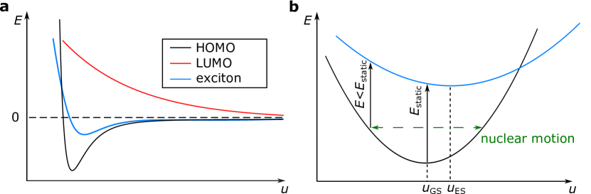
Figure 2: Schematic representation of the energy of the highest occupied (HOMO) and lowest unoccupied (LUMO) molecular orbitals, as well as the exciton state that results from a transition between them, along a generalized coordinate $u$ (panel a). Due to the excited state potential energy surface having a lower curvature, nuclear motion leads to a red-shift of the energy difference between the ground and excited states compared to its static value (panel b).

To simplify the problem of computing the exciton band maximum energy from equation 2, we use the harmonic approximation for the ground state potential, and by substituting $\ket{\chi_{\mathbf{s}}(\boldsymbol{u})}$ with the wavefunction of a quantum harmonic oscillator we obtain [18]:

$$E_{\text{exc}}(T)=\int d\boldsymbol{u}|\Phi(\boldsymbol{u};T)|^{2}E_{\text{exc}}(\boldsymbol{u}),$$ (4)

where $E_{\text{exc}}(\boldsymbol{u})$ is the vertical excitation energy at the configuration $\boldsymbol{u}$ and:

$$|\Phi(\boldsymbol{u};T)|^{2}=\prod_{\nu}(2\pi\sigma^{2}_{\nu}(T))^{-1/2}\exp{\left(-\frac{u_{\nu}^{2}}{2\sigma^{2}_{\nu}(T)}\right)},$$ (5)

is the harmonic density at temperature $T$, which in turn is a product of Gaussian functions of width:

$$\sigma^{2}_{\nu}(T)=\frac{1}{2\omega_{G\nu}}\cdot\coth{\left(\frac{\omega_{G\nu}}{2k_{B}T}\right)}.$$ (6)

In the above, atomic units and mass-weighted coordinates have been used, and $\nu$ is the index labeling the ground state vibrational modes of the studied molecule, with $\omega_{G\nu}$ the corresponding frequency. For non-linear molecular systems there are six vibrational modes with zero frequency which correspond to translations and rotations of the entire structure. These are not included in the sampling of the integral of equation 4.

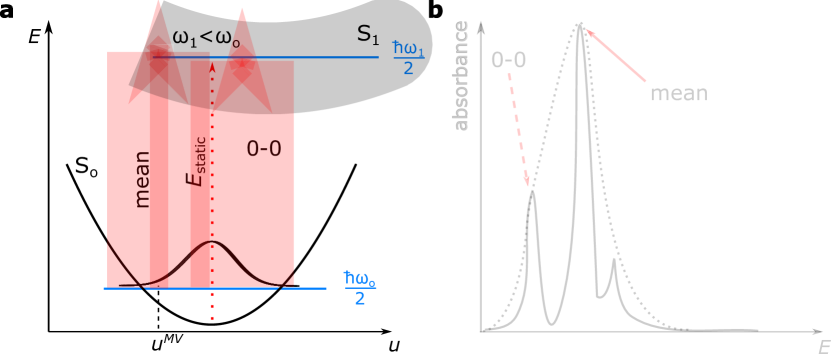
Figure 3: Vibrational effects result in a distribution of exciton energies (panel a, red shaded region) around a mean value, which is different to the ‘static’ exciton energy $E_{\text{static}}$. This can be represented as the vertical transition from the zero-point level of the ground state, to the excited state surface, at a ‘mean value’ configuration $u^{MV}$ (panel a). This mean energy of the excited state appears as the band maximum in experimental absorption spectra (panel b). In contrast to that, the $0-0$ energy refers to the energy difference between the zero-point levels of the optimized ground and excited states. These separate peaks cannot always be resolved experimentally, in which cases an envelope function (panel b, dotted lined) is found instead.

2.2 Monte Carlo sampling of the exciton energy

The Monte Carlo method approximates the integral in equation 4 by generating configurations $\boldsymbol{u}$ that are distributed according to the harmonic density at the temperature of choice $T$. Then, the expectation value of equation 4 is computed as the simple average of the computed values of the vertical exciton energy $E_{\text{exc}}(\boldsymbol{u})$ at the displaced configurations. This methodology for capturing the effect of vibrations on exciton energies has previously been applied in the context of periodic organic crystals [13], and here we extend it to isolated organic molecules. This computational approach has the advantage that it makes no assumption about the shape of the excited state potential energy surface and it also includes exciton-vibration interactions to all orders. Moreover, it relies on no adjustable parameters, apart from those in the DFT functional, which are fixed throughout the entire series of calculations. This Monte Carlo approach is conceptually very similar to the nuclear ensemble method [19], which was recently applied to the Thiel set of molecules [12], and we compare our results to this previous study later on, in Figure 5. For all the molecules studied we generate $100$ displaced configurations at $T=0$ K and $T=300$ K and their exciton energies are computed through TD-DFT within the Tamm-Dancoff approximation [28], using the popular B3LYP hybrid functional [29] and the cc-pVDZ basis set, as implemented within the NWChem code [30]. We hence obtain renormalized exciton energies compared to those of a ‘static’ TD-DFT calculation for the Thiel set of molecules. We generally find that approximately $50$ points are sufficient to sample the expectation value of the exciton energies (SI section S4). The numerical results of these calculations (and the associated statistical uncertainties) are given in SI section S1, not only at the B3LYP level, but also for two additional DFT functionals as discussed in subsection 3.2.

Since the Monte Carlo method provides an approximation to the expectation value of equation 2, we always compare the computed energy values to the absorption maximum which corresponds to the same exciton state (for example the first bright excited state), and not to the so-called $0-0$ energy (see also Figure 3). However, it is not uncommon that experimental works report the energy of the $0-0$ transition. For the vast majority of systems studied here, and unlike the schematic of Figure 3 which aims to emphasize the differences between these two quantities, the energies of the $0-0$ transition and the band maximum are either identical or very close to each other. Accurate explicit calculations of $0-0$ energies have been reported in the literature [31], and these require finding the optimized geometry of the excited state and computing its Hessian matrix, which can be very challenging computationally, especially for larger molecules such as the acene series and nucleobases, which are studied here. Given that the energy of the $0-0$ transition is in most cases very close, or even identical to that of the band maximum, the Monte Carlo method (and also the quadratic approximation which is outlined in the following subsection) could potentially be used to also approximate $0-0$ energies at a much lower computational cost.

2.3 The quadratic approximation

One can further simplify the expression of equation 4 by performing a quadratic expansion of the vertical excitation energy $E_{\text{exc}}(\boldsymbol{u})$ in the coordinates $u_{\nu}$ of the vibrational normal modes, yielding:

$$E_{\text{exc}}(\boldsymbol{u})=E_{\text{exc}}(\boldsymbol{0})+\sum_{\nu}\frac{\partial E_{\text{exc}}(\boldsymbol{0})}{\partial u_{\nu}}u_{\nu}+\frac{1}{2}\sum_{\nu}\sum_{\nu^{\prime}}\frac{\partial^{2}E_{\text{exc}}(\boldsymbol{0})}{\partial u_{\nu}\partial u_{\nu^{\prime}}}u_{\nu}u_{\nu^{\prime}}+...\hskip 2.84544pt.$$ (7)

Here $E_{\text{exc}}(\boldsymbol{0})$ is the exciton energy at the ground state geometry and is equal to the static exciton energy $E_{\text{static}}$ as defined previously. Substituting this expression in equation 4 gives:

$$E_{\text{exc}}(T)=E_{\text{static}}+\sum_{\nu}\frac{1}{2\omega_{\nu}}\cdot\frac{\partial^{2}E_{\text{exc}}}{\partial u_{\nu}^{2}}[\frac{1}{2}+n_{B}(\omega_{\nu},T)]+\mathcal{O}(u^{4}).$$ (8)

In equation 8, $n_{B}(\omega_{\nu},T)$ is the Bose-Einstein distribution for the vibrational quanta at temperature $T$. When computing the expectation value of the exciton energy in equation 8, all odd terms vanish due to the harmonic density $|\Phi(\boldsymbol{u};T)|^{2}$ being an even function, thus the resulting approximation is accurate to fourth order in $u$, and the exciton energy renormalization is described to lowest order by the quadratic term of the expansion. While this so-called quadratic approximation is in principle less accurate than the Monte Carlo approach which we outlined previously, it has the advantage of separating the contributions of the different vibrational normal modes to the exciton energy renormalization, potentially allowing for additional microscopic insights into these effects.

Equation 8 is used for calculations with the quadratic method, which essentially involves the calculation of the second derivative of the exciton energy along each vibrational mode of the system by using the finite difference formula:

$$\frac{\partial^{2}E_{\text{exc}}}{\partial u_{\nu}^{2}}\approx\frac{E_{\text{exc}}(\delta u_{\nu})+E_{\text{exc}}(-\delta u_{\nu})-2E_{\text{static}}}{\delta u_{\nu}^{2}}.$$ (9)

Hence two exciton energies at $\pm\delta u_{\nu}$ for each mode $\nu$, as well as the ‘static’ exciton energy $E_{\text{static}}$ need to be computed. For a molecule with $N$ atoms, this means that a total of $2\cdot(3N-6)+1$ exciton energy calculations are required, which for small molecules can be significantly smaller than the number of configurations required to converge a Monte Carlo calculation, a point that we return to in subsection 3.4. In principle, $\delta u$ is an infinitesimal quantity that should be as small as possible in the above finite difference formula, however in practice one needs to choose a finite value for this parameter in order to avoid numerical divergence issues. For perfectly quadratic energy surfaces the result would be independent of the displacement $\delta u$, and we can therefore conceptually extend the meaning of the quadratic formula to simply represent a finite displacement of the system along an individual vibrational mode. We return to this issue in subsection 3.4.

Finally, it is worth transforming equation 8 into a different form, which is not used for practical calculations within this work, but provides valuable intuition for the effects that we discuss. Let us assume the frequency of vibrational normal mode $\nu$ in the ground state to be equal to $\omega_{G\nu}^{2}$. If we further assume that this same normal mode is present in the excited state with a different frequency $\omega_{E\nu}^{2}$, then equation 8 becomes:

$$E(T)=E_{\text{static}}-\frac{1}{4}\sum_{\nu}\frac{\omega_{G\nu}^{2}-\omega_{E\nu}^{2}}{\omega_{G\nu}}[\frac{1}{2}+n_{B}(\omega_{\nu},T)]+\mathcal{O}(u^{4}),$$ (10)

This formula is identical to the one appearing in Ref. [32], where $E(T)$ is called first moment of the exciton. In the terms we have used here, the first moment is simply the expectation value of the exciton energy in the presence of molecular vibrations. Equation 10 demonstrates that the renormalization of the static exciton energy due to each normal mode depends on the frequency difference $\omega_{G\nu}^{2}-\omega_{E\nu}^{2}$, and suggests that $E(T)<E_{\text{static}}$ as long as the potential energy surface of the ground state has a higher curvature than that of the excited state and therefore $\omega_{G\nu}^{2}>\omega_{E\nu}^{2}$. This analytical result is essentially the mathematical manifestation of the intuitive picture of Figure 2, and holds in the general multi-dimensional case, at least within the validity of the quadratic approximation.

3 Results and discussion

3.1 Comparison to published results

We compare the energies of the singlet excitons obtained within our Monte Carlo approach by computing exciton energies at the B3LYP level of TD-DFT and including the effects of zero-point renormalization (ZPR), to the experimental values for the corresponding maxima. The references to the experimental works are summarized in SI section S2. These same references were collected in the original publication on the Thiel set [22], however the values can be slightly different for a few of the studied molecules, as we had to ensure that we compare to the band maximum in every case. We also compare the values obtained from ‘static’ TD-DFT and from highly accurate complete active space second-order perturbation theory (CASPT2) [33] calculations in the original Thiel publication [22] to experiment. The computed exciton energies always refer to the first single excitation as described within TD-DFT, and we exclude any double-excitations (bi-excitons) from our analysis, which are however accessible using wavefunction-based methods [22]. In Figure 4 we plot the computed versus experimental values for the three approaches, for all the studied molecules for which experimental data is given in Ref. [22]. The closer a point lies to the $y=x$ line, the better the agreement between theory and experiment. We fit a linear model to the three sets of results, as a means of visualizing the overall agreement with experiment, from where it becomes evident that the TD-DFT B3LYP+ZPR (red) results provide a significant improvement to the static TD-DFT B3LYP values (green). The numerical results of the Monte Carlo simulations for the exciton energy renormalization are summarized in SI section S1, along with the associated statistical uncertainties. The parameters for all the linear fits are given in SI section S2. Naturally the Thiel values (black), which were obtained using accurate wavefunction-based methods and capture correlation effects, provide an improvement to static TD-DFT. However, from Figure 4 it is evident that the correction to TD-DFT exciton energies induced by the quantum fluctuations of molecular vibrations is at least as significant as their correction due to the correlation effects included in the Thiel calculations, at least for the specific set of molecules we study here. From Figure 4 it also becomes obvious that the ZPR of exciton energies can become very large, with values that can be as high as $1.362$ eV in the case of pyrrole. The average correction is found to be $(345\pm 67)$ meV, which is substantial and certainly needs to be accounted for in order for exciton energy calculations to achieve predictive accuracy. We have also investigated the effect of increasing the temperature from $0$ K to $300$ K, however we found that for the vast majority of molecules the resulting difference in the exciton energy is small, as summarized in SI section S3. This is intuitively obvious from the fact that small organic molecules are dominated by high-frequency vibrational modes such as carbon-carbon stretching motions, which generally lie significantly above the threshold for thermal activation at room temperature.

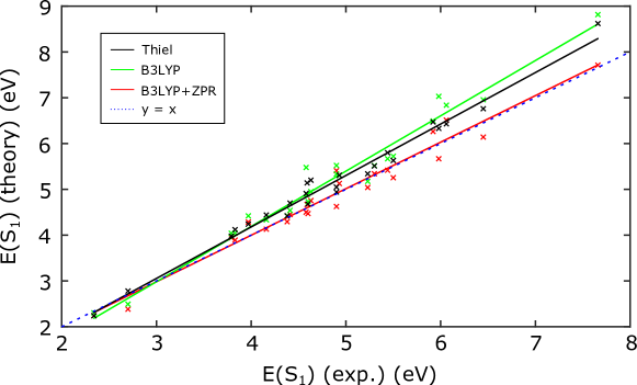
Figure 4: Comparison of the different methods used to obtain the singlet exciton energies of the Thiel set to experiment. A ‘static’ TD-DFT approach at the B3LYP level (green) performs the worst, and accurate wavefunction-based methods reported in the literature (black) improve overall agreement (the values in black refer to the CASPT2 Thiel values [22] for single excitations, corresponding to the states computed within TD-DFT here). However, accounting for the zero-point renormalization (ZPR) of exciton energies due to molecular quantum fluctuations leads to the best agreement with experiment (red), even when ignoring beyond-TD-DFT electronic effects.

	bias (eV)	rel.bias	RMSE (eV)	rel.RMSE
B3LYP	$0.343$	$0.0673$	$0.495$	$0.091$
Thiel	$0.283$	$0.0545$	$0.357$	$0.067$
B3LYP+ZPR	$0.011$	$0.0003$	$0.231$	$0.050$

Table 1: Statistical measures of the accuracy of the different methods. The average values of the (relative) bias and the (relative) root mean-squared error (RMSE) as defined in the text are given. The comparisons to experiment refer to the $24$ molecules for which experimental data was found (see SI section S2).

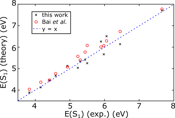
Figure 5: Comparison of the exciton energies obtained within our Monte Carlo approach employing TD-DFT and accounting for nuclear quantum effects (B3LYP+ZPR), to the values reported in Ref. [12] using the nuclear ensemble method in conjunction with coupled cluster calculations. Both methods lead to excellent agreement with experiment.

	bias (eV)	rel.bias	RMSE (eV)	rel.RMSE
Bai et al. [12]	$0.211$	$0.040$	$0.250$	$0.047$
This work	$0.011$	$0.003$	$0.218$	$0.037$

Table 2: Statistical measures of the accuracy of our work within a Monte Carlo (B3LYP+ZPR) approach and the results reported in [12] using the nuclear ensemble method combined with coupled cluster calculations. The average values of the (relative) bias and the (relative) root mean-squared error (RMSE) as defined in the text are given. The comparison is restricted to the structures for which the same exciton state has been studied in our work and in Ref. [12].

We employ four different statistical measures in order to rigorously compare the accuracy of the different methods presented in Figure 4, which we summarize in Table 1. In particular, for our $n=24$ studied molecules with computed exciton energies $b_{i}$ and experimental exciton energies $a_{i}$, we compute the average values of the bias: $\text{bias}=\frac{1}{n}\sum_{i}(b_{i}-a_{i})$, the root mean-squared error: $\text{RMSE}=\sqrt{\frac{1}{n}\sum_{i}(b_{i}-a_{i})^{2}}$, as well as the relative values to these quantities: $(\text{rel.bias})=\frac{1}{n}\sum\frac{b_{i}-a_{i}}{a_{i}}$, $(\text{rel.RMSE})=\sqrt{\frac{1}{N}\sum_{i}\frac{(b_{i}-a_{i})^{2}}{a_{i}^{2}}}$. The reason that we also consider the relative quantities is that the largest errors for the static TD-DFT and Thiel approaches are found in the region of large exciton energies, hence these molecules dominate the bias and root mean-squared error. For example, the static TD-DFT exciton energy of ethene is renormalized from $8.8$ eV to $7.7$ eV once we account for nuclear quantum effects. Using the relative bias and root mean-squared error, which are calculated by dividing by $a_{i}$ and $a_{i}^{2}$ respectively, we achieve a fairer comparison without under-representing the effect of molecules with lower exciton energies. We see from Table 1 that the average value of all the employed statistical measures is minimized when using TD-DFT at the B3LYP level combined with the zero-point renormalization (B3LYP+ZPR) of exciton energies due to molecular vibrations. We therefore quantitatively confirm the observation of Figure 4: for the studied set of molecules, corrections to static exciton energies due to nuclear quantum motion are generally larger than corrections due to beyond-TD-DFT electronic effects that are included in the Thiel values. We also quantify the spread of the four statistical quantities around their average value by computing their standard deviation, which is given in SI Table S32. We find that the spread of the B3LYP+ZPR values is in every case comparable to that of the Thiel values, and significantly smaller than that of the static TD-DFT (B3LYP) values.

Similar results to ours were presented in Ref. [12] using the nuclear ensemble method and coupled cluster calculations, although the computed values were not compared to experiment in that case. In Figure 5 we compare our results obtained within the Monte Carlo method at the TD-DFT level to those of Ref. [12]. We restrict the comparison to fourteen structures for which the same exciton state has been studied, as Ref. [12] also reports the energies of some excitons that are not necessarily the lowest-lying ones, which we chose to study in this work. We see that both computational methods lead to excellent agreement with experiment, and a rigorous comparison is made in Table 2. Among the reported statistical measures, the RMSE and relative RMSE are the ones that most accurately capture the accuracy of the two methods, as they do not suffer from effects such as cancellations of errors, which are evidently present in the bias and relative bias when using TD-DFT due to some values underestimating and some others overestimating experiment. This is not a problem with coupled cluster calculations in the studied molecules, since these generally predict an exciton energy value that is higher compared to TD-DFT, which also becomes apparent from the fact that the values in Ref. [12] tend to slightly overestimate experiment, as seen in Figure 5. Since the agreement of our results within TD-DFT to experiment is comparable to the agreement of the results of Bai et al. which were obtained using coupled cluster calculations, it is once again highlighted that at least for the specific set of studied molecules, the ZPR of exciton energies provides a larger, or at least comparable, correction to the static TD-DFT exciton energies compared to the correction obtained by using more accurate electronic structure methods. Of course it is still generally the case that one needs both an accurate description of the electronic structure and of vibrational effects in order to achieve better quality results. To demonstrate this fact, we have chosen four molecules for which TD-DFT calculations at the B3LYP level provide a poor starting point for the static exciton energy, as well as inaccurate values once ZPR is accounted for, and we now perform a Monte Carlo sampling by employing significantly more accurate coupled cluster singles and doubles (CCSD) calculations. These molecules are benzoquinone, cyclopropene, formamide, and pyrrole, and the results are summarized in Table 3. In all cases, the corrected exciton energy obtained by using CCSD calculations within our Monte Carlo sampling is closer to the experimental value compared to the TD-DFT case. However, even in this case the experimental values for benzoquinone and cyclopropene are overestimated by $0.2-0.3$ eV. We attribute this behavior to the still limited treatment of correlations within CCSD compared to more accurate methods, which results in these calculations commonly overestimating excited state energies as also observed in the results of Ref. [12] shown in Figure 5.

molecule	B3LYP	B3LYP+ZPR	CCSD	CCSD+ZPR	experiment
benzoquinone	$2.493$	$2.383(15)$	$3.126$	$2.999(15)$	$2.7$ [34]
cyclopropene	$6.956$	$6.141(30)$	$7.508$	$6.663(32)$	$6.45$ [35]
formamide	$5.722$	$5.254(57)$	$5.876$	$5.456(56)$	$5.5$ [36]
pyrrole	$7.030$	$5.668(43)$	$6.822$	$5.935(78)$	$5.98$ [37]

Table 3: Comparison of the energy of the first excited state computed at the different levels of theory to experimental values. For the cases where zero-point renormalization (ZPR) is computed, the associated statistical uncertainty of the final exciton energy is given in parenthesis.

3.2 Exciton energy renormalization at different levels of theory

Ideally, one would combine accurate electronic structure calculations with our approach for accounting for nuclear quantum motion. However, for most of the studied molecules we found that a minimum of approximately $50$ points is required to converge the Monte Carlo sampling of the integral in equation 4. While the cost of $50$ TD-DFT calculations of small molecules is reasonably low, it quickly becomes very high as one moves to more accurate wavefunction-based methods. It is therefore reasonable to wonder whether the vibrational corrections to exciton energies could be computed at one (cheaper) level of theory and applied to the static exciton energy obtained at another (more accurate) level of theory. Some first conclusions on this can be drawn from the comparison of the excited state energy corrections at the TD-DFT B3LYP and CCSD levels of Table 3; with the exception of pyrrole for which the B3LYP correction is $1.5$ times larger than the CCSD one, the maximum deviation of the B3LYP zero-point renormalization from the CCSD value is $13\%$. While of course this is encouraging, these data points alone are not enough to draw a general conclusion. However, given this good agreement between the few B3LYP and CCSD excited state energy corrections that we compared, the fact that hybrid functionals such as B3LYP are known to lead to an accurate description of the electron-vibration interactions in organic molecules [38], and also the excellent agreement between theory and experiment in Figure 4, it seems a reasonable conclusion that hybrid functionals provide an accurate description of exciton-vibration coupling and the zero-point renormalization this induces.

In order to check whether the vibrational correction to exciton energies changes when using different electronic structure methods in a more systematic manner, we repeated our Monte Carlo sampling using the local density approximation (LDA) and pure Hartree-Fock (HF) exchange within TD-DFT, while using the vibrational modes obtained at the B3LYP level. This choice of functionals allows us to comment on the role of exact exchange for exciton-vibration interactions: in particular, LDA includes no exact exchange, while B3LYP includes $20\%$ and HF represents the case of including full exact exchange. Since the included fraction of exchange is generally known to have little effect on the structure of a molecule and the computed ground-state vibrational modes [38], using the B3LYP geometries and vibrational modes is a reasonable approximation. Therefore, all differences in the values of the exciton energy renormalization between the different functionals are purely due to the variations of the excited state wavefunction as obtained from TD-DFT.

The numerical results of the calculations employing the different functionals are presented in SI section S1. We compare the LDA and HF energy corrections to the B3LYP ones and find that on average, LDA predicts a red-shift of the excited state energy which is $1.3$ times greater than B3LYP, and HF $1.8$ times greater. This is in agreement with reports on electron-vibration interactions being strongly affected by the fraction of exact exchange included in the calculation [38]. The results suggest that LDA provides a reasonable approximation to B3LYP for computing zero-point renormalization in the studied organic molecules, with only a few structures showing very strong deviations. As shown in SI Figure S1, the largest differences between the corrections predicted by LDA and B3LYP are found for smaller molecules with less than $60$ electrons. We attribute this observation to the fact that the excited states of these smaller structures have a greater electronic density in the vicinity of the localized high-frequency vibrations that can dominate in organics, hence leading to a very strong coupling that is very sensitive to the detailed structure of the excited state wavefunction. These points are revisited in subsections 3.3 and 3.5 where the impact of molecular size and individual vibrational modes on zero-point renormalization are discussed respectively.

Overall, we find that in most organic structures, hybrid functionals such as B3LYP provide a good approximation to the values of zero-point renormalization computed with more accurate methods such as CCSD. For several of the studied molecules, even the complete omission of exact exchange through the use of LDA seems to also give reasonable results within $30\%$ of the B3LYP values. Most strong deviations between electronic structure methods are found for smaller molecules, which is in a sense encouraging, since these are the ones that can commonly be studied using more expensive methods without too great of a computational cost.

3.3 The impact of the molecular size

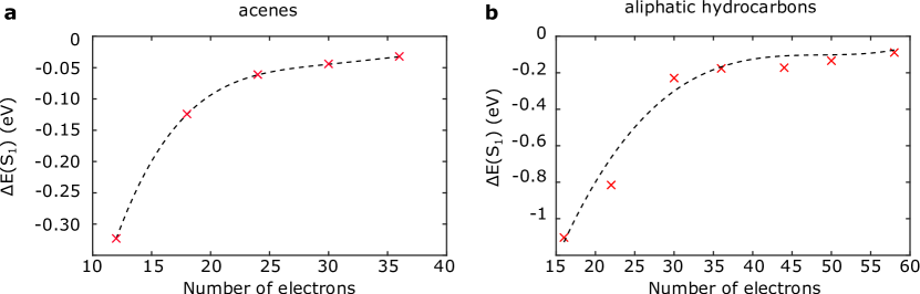
Figure 6: Size dependence of the correction $\Delta\text{E}(\text{S}_{1})$ that nuclear quantum motion induces to the singlet exciton energies of the acene (panel a) and aliphatic hydrocarbon (panel b) families of molecules.

We found in Ref. [13] for periodic molecular crystals that the correction to exciton energies due to nuclear quantum motion becomes more important for smaller molecules. For the single-molecule systems studied here we find that the same trend holds, as shown in Figure 6 for the acene and aliphatic hydrocarbons families of molecules. The results in Figure 6 are obtained at the TD-DFT B3LYP level of theory. We believe that the reason for the observed trend is that smaller molecules have a greater electronic density in the vicinity of localized atomic motions that are activated due to quantum fluctuations, hence leading to stronger exciton-vibration interactions. Another way of reaching the same conclusion is using Hückel theory. Let us consider the example of linear polyenes, such as ethene, butadiene, hexatriene and octatetraene that are studied here and are included among other aliphatic hydrocarbons in Figure 6b, showing a decrease in the exciton energy correction with increasing system size. For a linear polyene consisting of $N$ carbon atoms, Hückel theory predicts the energy of the $i^{\text{th}}$ orbital is: $E_{i}=\alpha+2\beta\cos{(2\pi n/(N+1))}$, with $\alpha,\beta$ the Hückel parameters, and $i=1,2,...,N$. From this, we find for the HOMO-LUMO gap:

$$E_{\text{gap}}\propto\sin(\frac{\pi}{2(N+1)}).$$ (11)

In the limit of $N\rightarrow\infty$, this gives $E_{\text{gap}}\propto 1/N$. A similar result can be obtained for cyclic polyenes. Assuming that the same holds for any general conjugated molecule, this suggests that in larger systems the HOMO is less bonding and the LUMO less anti-bonding than in comparably smaller systems. Therefore, from the intuitive picture of Figure 2, the curvature of the ground and excited state surfaces of large molecules is similar, and the difference in their normal mode frequencies is small. Hence, according to the expression 10 that results from the quadratic approximation, the correction to the exciton energy is also smaller than that for a smaller molecule. This is encouraging, in the sense that corrections due to nuclear quantum motion are mostly important for small systems, for which they are cheaper to compute.

3.4 Accuracy and speed of the quadratic method

Having established the accuracy of the Monte Carlo method for computing the exciton energy renormalization due to nuclear quantum motion, we now proceed to use it as a benchmark to assess the accuracy of the quadratic method. Figure 7 visualizes the quadratic versus the Monte Carlo correction for each of the studied molecules, using TD-DFT and the B3LYP functional, along with the cc-pVDZ basis set. The better the agreement between the two methods for a given molecule, the closer the associated point lies to the $y=x$ line (dashed line). Overall, the agreement between the two methods is good, and we propose that the quadratic method can indeed be used to make quantitative predictions of exciton energies including vibrational renormalization effects. Particularly for smaller molecules, this has the additional advantage that it comes at a lower computational cost compared to Monte Carlo sampling (see also theoretical background section and the discussion accompanying Figure 9 below). The converged values for the exciton energies as predicted by the quadratic method are summarized in SI section S5.

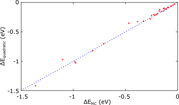
Figure 7: Comparison of values predicted by the quadratic and Monte Carlo methods for the zero-point renormalization of the exciton energy of the different molecules. The $y=x$ line is given in blue for reference.

As already mentioned in subsection 2.3, when computing the quadratic correction to the exciton energies, one needs to make a choice for the displacement $\delta u$ appearing in equation 8. We find that generally a displacement of $\delta u=\sigma$, where $\sigma$ is the standard deviation of the thermal quantum distribution appearing in equation 6, leads to results that are in very close agreement with the computed Monte Carlo values. Figures 8a and 8b show the quadratic correction of pyrazine and tetracene respectively, comparing the quadratic values at different values of $\delta u$ (red crosses) with the Monte Carlo correction (blue line) and its associated statistical uncertainty (blue shaded region). The variation of the quadratic correction due to changes in $\delta u$ is generally comparable to the statistical uncertainty of the Monte Carlo method.

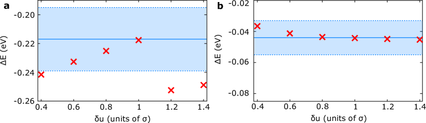
Figure 8: Zero-point renormalization $\Delta E$ of the exciton energy predicted by the quadratic method, with respect to the displacement $\delta u$ appearing in equation 8), for the case of pyrazine (panel a) and tetracene (panel b). The energy shift predicted by the Monte Carlo approach is given for reference (blue line) and its statistical uncertainty indicated with the blue shaded region.

We also explore the computational cost of the quadratic method and compare to that of a Monte Carlo sampling. In Figure 9 we visualize the CPU hours required to compute the correction to the static exciton energies that is induced by the zero-point motion of the different molecules. For the Monte Carlo sampling, the calculation always includes taking an average over $100$ configurations as mentioned previously, which we find leads to converged results and small statistical uncertainties to the final exciton energies (SI section S4). Overall, the quadratic method is cheaper to use for smaller structures with fewer electrons, where we also argue that the correction to exciton energies due to vibrations is larger (see Figure 6 and discussion). Therefore, given also the accuracy of this method and the mode-resolved information it provides (see subsection 3.5), we propose that it is the better alternative once one approaches the limit of smaller molecules. For larger structures with several vibrational normal modes we find that the Monte Carlo method provides a faster estimate of the red-shift and should thus be preferred.

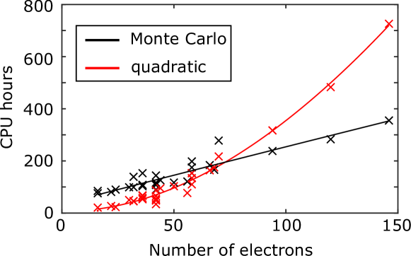
Figure 9: Comparison of the CPU hours required to compute the exciton energy correction of the different molecules due to nuclear quantum motion, using the Monte Carlo (black crosses) and quadratic (red crosses) methods. The solid lines are given as guides to the eye.

3.5 Mode-resolved picture for the exciton energy renormalization

While the quadratic method for computing the renormalization of exciton energies due to quantum fluctuations is in principle less accurate than performing a Monte Carlo sampling, it is a cheaper and simpler method that is easier to implement computationally. However, perhaps its most important advantage is the fact that it separates the contributions of the individual vibrational normal modes to the exciton energy renormalization, as revealed by equation 8. In Figures 10b and 11b we visualize the mode-resolved renormalization of the exciton energy of pyrazine and ethene respectively, at $T=0$ K. From these figures, it becomes evident that for both molecules, it is only a few modes that dominate the zero-point renormalization of the exciton energy. In both cases, the most important mode for the exciton energy renormalization is highlighted in a red circle. For pyrazine, this dominant mode is responsible for $35$% of the exciton energy renormalization, while for ethene for $56$%.

In order to gain a deeper microscopic understanding of the effect of the specific vibrational modes on the exciton states of these molecules, we plot the undistorted ‘static’ exciton wavefunctions (represented by the transition density) in Figures 10a and 11a respectively, together with the wavefunction at a typical distorted configuration ($\delta u=\sigma$) along these dominant modes, visualized in Figures  10d and 11d. For comparison, we also plot the exciton wavefunction when the molecule is displaced along a mode which is weakly coupled to the exciton in Figures 10c and 11c, together with the displacement pattern of these motions. These weakly coupled vibrational modes are highlighted in green in Figures 10b and 11b. It is evident that while the displacement of the dominant modes leads to a significant change of the excitonic wavefunction from its form at the equilibrium geometry, this is not the case for weakly coupled modes.

The dominating modes for exciton renormalization can sometimes be qualitatively explained from a chemically intuitive perspective by considering the conventional skeletal structures of the ground and excited state molecules, and (from equation 10) which stretching modes are likely to be far weaker (lower frequency) in the excited state compared to the ground state. For pyrazine in Figure 10, as an aromatic molecule similar to benzene, it has two principal resonance structures as shown in Figure 10e. The HOMO and LUMO are both $\pi$ orbitals and excitation to $\text{S}_{1}$ can be qualitatively drawn as breaking a $\pi$ bond, leading to a (singlet) biradical. The biradical [39] has numerous possible resonance structures, three of which are drawn in Figure 10e. These quinoidal structures suggest that in the $\text{S}_{1}$ state, for a given nitrogen it will be easier to elongate one C-N bond while shortening the other to form a quinoidal-like biradical. This corresponds to the dominant stretching vibration in Figure 10d.

Similarly, for ethene in Figure 11, in the ground $\text{S}_{0}$ state the molecule is planar due to the $\pi$ bond, although this causes some small steric hindrance between hydrogen atoms of different carbons. Upon exciting to the $\text{S}_{1}$ state, the $\pi$ bond is broken, such that it is much easier to rotate around the central C-C bond as shown in Figure 11e and we would expect the frequency of this mode to drastically reduce, leading to a large renormalization by equation 10. This rotation is the dominating mode as shown in Figure 11d.

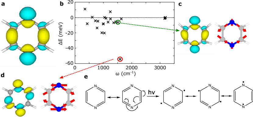
Figure 10: Mode-resolved zero-point renormalization of the exciton energy of pyrazine. The renormalization of the exciton energy due to the various normal modes of vibration is given in panel b, with a weakly coupled mode highlighted in green (displacement pattern in panel c), and the most strongly coupled mode highlighted in red (displacement pattern in panel d). The exciton wavefunction (transition density) is visualized in panel a in the optimized geometry, and along the weakly and strongly coupled modes in panels c and d respectively. The resonance structures of pyrazine in the ground state and upon photoexcitation are shown in panel e.

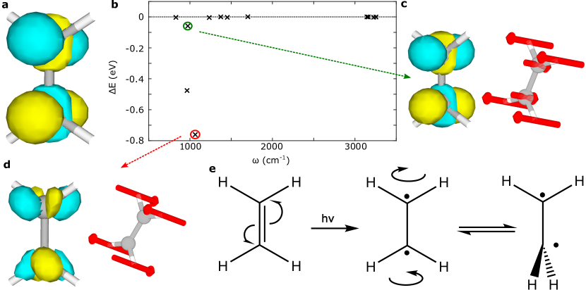
Figure 11: Mode-resolved zero-point renormalization of the exciton energy of ethene. The renormalization of the exciton energy due to the various normal modes of vibration is given in panel b, with a weakly coupled mode highlighted in green (displacement pattern in panel c), and the most strongly coupled mode highlighted in red (displacement pattern in panel d). The exciton wavefunction (transition density) is visualized in panel a in the optimized geometry, and along the weakly and strongly coupled modes in panels c and d respectively. The resonance structures of ethene in the ground state and upon photoexcitation are shown in panel e.

It is not always true that a subset of modes can be identified to dominate the exciton energy renormalization, however some patterns can still be observed. Perhaps the most obvious one is a ring-breathing mode of frequency in the vicinity of $1600$ $\text{cm}^{-1}$, which is largely responsible for the exciton energy renormalization in several cyclic compounds, which can be intuitively understood as in the case of pyrazine in Figure 10e, where this motion contributes $35\%$ of the renormalization. Similarly for other cyclic structures: benzoquinone ($20$%), pyridine ($38$%), pyrimidine ($39$%), tetrazine ($62$%) and triazine ($30$%). For each of the studied molecules, we give the percentage of contribution of the mode that most strongly couples to the exciton energy renormalization, along with the frequency of this motion, in SI section S5. Overall, in most molecules high-frequency modes dominate the renormalization of exciton energies, with the average frequency of the most strongly coupled mode being $\bar{\omega}_{\text{dominant}}=(1024\pm 121$) $\text{cm}^{-1}$. This dominance of high-frequency modes is consistent with our observation of subsection 3.3 that zero-point renormalization is, for the molecules studied here, more prominent in smaller molecular structures. The excited states of these systems have a greater electronic density in the vicinity of localized high-frequency motions, such as carbon-carbon stretches, hence the corresponding wavefunctions show stronger variations upon displacement of the atoms. It is for the same reasons that larger differences in the computed energy corrections between the different functionals tend to appear for smaller molecular structures, as was seen in subsection 3.2; the strong exciton-vibration interactions in these systems can be very sensitive to the local structure of the excited state wavefunctions, which depends on the level of electronic structure theory.

4 Conclusions

In this work we have presented an intuitive picture for the red-shift of exciton energies that is caused by nuclear quantum motion, and two computational approaches for estimating its magnitude. We find that this red-shift can indeed be very substantial, reaching values of more than $1$ eV in some cases. We rigorously compare our results for the exciton energies of a large set of molecules, obtained within a Monte Carlo framework and time-dependent density functional theory, to experiment and previous computational studies, and find that accounting for the effects of nuclear quantum motion in this manner leads to predictive accuracy for exciton energies. We show that the magnitude of the red-shift provided by quantum fluctuations is typically larger for smaller molecules, a result which we explain within a Hückel theory picture. Moreover, we find that while the predicted red-shift caused by vibrations depends on the level of theory used for the exciton calculations, TD-DFT employing hybrid functionals should provide a good compromise between accuracy and computational cost for estimating its magnitude. Naturally, further improvement of the results can be achieved by combining our Monte Carlo approach with more accurate methods of electronic structure calculations, such as coupled cluster, as we also demonstrate for a subset of the studied molecules. Additionally, we employ a quadratic approximation for computing the magnitude of exciton energy renormalization due to zero-point motion, which allows us to disentangle the contribution of individual normal modes to this effect. While this method is conceptually easier to implement compared to a Monte Carlo sampling, it is in principle less accurate as well. Nevertheless, we find that it performs very well for the diverse set of molecules which are studied here, and it also provides a cheaper way of computing the renormalization of exciton energies in smaller molecules, where this effect is also most relevant. By using the quadratic method we find that for several molecules the renormalization of the exciton energy is dominated by a few normal modes of vibration, with a ring-breathing motion playing a prominent role in the red-shift of the exciton energy in several cyclic compounds. Overall, our study provides critical microscopic insights into the effect of nuclear quantum motion on exciton energies at equilibrium, and emphasizes its importance for achieving predictive accuracy.

Supplementary Material

See supplementary material for the full results of the Monte Carlo sampling using different functionals, details for the comparison of these results to experiment, convergence tests and results at $300$ K. Detailed data on the vibrational modes dominating the quadratic correction of the exciton energy are also provided.

Data availability

The data that support the findings of this study are openly available in Apollo, the University of Cambridge repository, at https://doi.org/10.17863/CAM.70585, reference number [40].

References

- [1] J. Frenkel. On the transformation of light into heat in solids. I. Physical Review, 37:17–44, 1931.
- [2] Akshay Rao and Richard H Friend. Harnessing singlet exciton fission to break the Shockley–Queisser limit. Nature Reviews Materials, 2:17063, October 2017.
- [3] Antonios M. Alvertis, Steven Lukman, Timothy J H Hele, Eric G Fuemmeler, Jiaqi Feng, Jishan Wu, Neil C Greenham, Alex W Chin, and Andrew J Musser. Switching between Coherent and Incoherent Singlet Fission via Solvent-Induced Symmetry Breaking. Journal of the American Chemical Society, 141:17558, 2019.
- [4] Sebastian Reineke. Organic light-emitting diodes: Phosphorescence meets its match. Nature Photonics, 8(4):269–270, 2014.
- [5] Emrys W. Evans, Yoann Olivier, Yuttapoom Puttisong, William K. Myers, Timothy J.H. Hele, S. Matthew Menke, Tudor H. Thomas, Dan Credgington, David Beljonne, Richard H. Friend, and Neil C. Greenham. Vibrationally Assisted Intersystem Crossing in Benchmark Thermally Activated Delayed Fluorescence Molecules. Journal of Physical Chemistry Letters, 9(14):4053–4058, 2018.
- [6] M. Petersilka, U. J. Gossmann, and E. K.U. Gross. Excitation energies from time-dependent density-functional theory. Physical Review Letters, 76(8):1212–1215, 1996.
- [7] Rodney J. Bartlett. Coupled-cluster approach to molecular structure and spectra: A step toward predictive quantum chemistry. Journal of Physical Chemistry, 93(5):1697–1708, 1989.
- [8] Per Åke Malmqvist and Björn O. Roos. The CASSCF state interaction method. Chemical Physics Letters, 155(2):189–194, 1989.
- [9] Michael Rohlfing and Steven G. Louie. Electron-hole excitations and optical spectra from first principles. Physical Review B - Condensed Matter and Materials Physics, 62(8):4927–4944, 2000.
- [10] Denis Jacquemin, Ivan Duchemin, and Xavier Blase. Benchmarking the Bethe-Salpeter Formalism on a Standard Organic Molecular Set. Journal of Chemical Theory and Computation, 11(7):3290–3304, 2015.
- [11] Denis Jacquemin, Ivan Duchemin, Aymeric Blondel, and Xavier Blase. Benchmark of Bethe-Salpeter for Triplet Excited-States. Journal of Chemical Theory and Computation, 13(2):767–783, 2017.
- [12] Shuming Bai, Ritam Mansour, Ljiljana Stojanović, Josene M. Toldo, and Mario Barbatti. On the origin of the shift between vertical excitation and band maximum in molecular photoabsorption. Journal of Molecular Modeling, 26(5), 2020.
- [13] Antonios M. Alvertis, Raj Pandya, Loreta A. Muscarella, Nipun Sawhney, Malgorzata Nguyen, Bruno Ehrler, Akshay Rao, Richard H. Friend, Alex W. Chin, and Bartomeu Monserrat. Impact of exciton delocalization on exciton-vibration interactions in organic semiconductors. Physical Review B - Condensed Matter and Materials Physics, 102:081122(R), 2020.
- [14] Fabrizio Santoro, Roberto Improta, Alessandro Lami, Julien Bloino, and Vincenzo Barone. Effective method to compute franck-condon integrals for optical spectra of large molecules in solution. The Journal of Chemical Physics, 126(8):084509, 2007.
- [15] Azzam Charaf-Eddin, Thomas Cauchy, François Xavier Felpin, and Denis Jacquemin. Vibronic spectra of organic electronic chromophores. RSC Advances, 4(98):55466–55472, 2014.
- [16] Alberto Baiardi, Julien Bloino, and Vincenzo Barone. General time dependent approach to vibronic spectroscopy including franck-condon, herzberg-teller, and duschinsky effects. Journal of Chemical Theory and Computation, 9(9):4097–4115, 2013.
- [17] K. Kunc and Richard M. Martin. Ab initio force constants of GaAs: A new approach to calculation of phonons and dielectric properties. Physical Review Letters, 48(6):406–409, 1982.
- [18] Bartomeu Monserrat. Electron – phonon coupling from finite differences. Journal of Physics Condensed Matter, 30, 2018.
- [19] Rachel Crespo-Otero and Mario Barbatti. Spectrum simulation and decomposition with nuclear ensemble: Formal derivation and application to benzene, furan and 2-phenylfuran. Theoretical Chemistry Accounts, 131(6):1–14, 2012.
- [20] Antonios M. Alvertis, Florian A.Y.N. Schröder, and Alex W. Chin. Non-equilibrium relaxation of hot states in organic semiconductors: Impact of mode-selective excitation on charge transfer. Journal of Chemical Physics, 151(8), 2019.
- [21] Shahnawaz Rafiq, Bo Fu, Bryan Kudisch, and Gregory D. Scholes. Interplay of vibrational wavepackets during an ultrafast electron transfer reaction. Nature Chemistry, 13(1):70–76, 2021.
- [22] Marko Schreiber, Mario R. Silva-Junior, Stephan P.A. Sauer, and Walter Thiel. Benchmarks for electronically excited states: CASPT2, CC2, CCSD, and CC3. Journal of Chemical Physics, 128(13), 2008.
- [23] Subhayan Roychoudhury, Stefano Sanvito, and David D. O’Regan. Neutral excitation density-functional theory: an efficient and variational first-principles method for simulating neutral excitations in molecules. Scientific Reports, 10(1):1–12, 2020.
- [24] Fabien Bruneval, Samia M. Hamed, and Jeffrey B. Neaton. A systematic benchmark of the ab initio Bethe-Salpeter equation approach for low-lying optical excitations of small organic molecules. Journal of Chemical Physics, 142(24), 2015.
- [25] Tonatiuh Rangel, Samia M. Hamed, Fabien Bruneval, and Jeffrey B. Neaton. An assessment of low-lying excitation energies and triplet instabilities of organic molecules with an ab initio Bethe-Salpeter equation approach and the Tamm-Dancoff approximation. Journal of Chemical Physics, 146(19), 2017.
- [26] Peter William Atkins. Molecular quantum mechanics. Oxford University Press, New York, 4th edition, 2005.
- [27] Bartomeu Monserrat. Vibrational averages along thermal lines. Physical Review B, 93(1):1–10, 2016.
- [28] So Hirata and Martin Head-Gordon. Time-dependent density functional theory within the Tamm-Dancoff approximation. Chemical Physics Letters, 314(3-4):291–299, 1999.
- [29] Axel D. Becke. A new mixing of Hartree-Fock and local density-functional theories. The Journal of Chemical Physics, 98(2):1372–1377, 1993.
- [30] E. Aprà et al. NWChem: Past, present, and future. The Journal of chemical physics, 152(18):184102, 2020.
- [31] Pierre François Loos, Nicolas Galland, and Denis Jacquemin. Theoretical 0-0 Energies with Chemical Accuracy. Journal of Physical Chemistry Letters, 9(16):4646–4651, 2018.
- [32] Francisco J.Avila Ferrer, Javier Cerezo, Emiliano Stendardo, Roberto Improta, and Fabrizio Santoro. Insights for an accurate comparison of computational data to experimental absorption and emission spectra: Beyond the vertical transition approximation. Journal of Chemical Theory and Computation, 9(4):2072–2082, 2013.
- [33] Kerstin Andersson, Per Åke Malmqvist, Björn O. Roos, Andrzej J. Sadlej, and Krzysztof Wolinski. Second-order perturbation theory with a CASSCF reference function. Journal of Physical Chemistry, 94(14):5483–5488, 1990.
- [34] Johannes Weber, Karsten Malsch, and Georg Hohlneicher. Excited electronic states of p-benzoquinone. Chemical Physics, 264(3):275–318, 2001.
- [35] M. B. Robin, Harold Basch, N. A. Kuebler, K. B. Wiberg, and G. B. Ellison. Optical spectra of small rings. ii. the unsaturated three‐membered rings. The Journal of Chemical Physics, 51(1):45–52, 1969.
- [36] Leigh B Clark. Polarization Assignments in the Vacuum UC Spectra of the Primary Amide, Carboxyl, and Peptide Groups. Journal of the American Chemical Society, 117:7974–7986, 1995.
- [37] Wayne M. Flicker, Oren A. Mosher, and Aron Kuppermann. Electron impact investigation of electronic excitations in furan, thiophene, and pyrrole. The Journal of Chemical Physics, 64(4):1315–1321, 1976.
- [38] Jonathan Laflamme Janssen, Michel Côté, Steven G. Louie, and Marvin L. Cohen. Electron-phonon coupling in C60 using hybrid functionals. Physical Review B - Condensed Matter and Materials Physics, 81(7):2–5, 2010.
- [39] Thijs Stuyver, Bo Chen, Tao Zeng, Paul Geerlings, Frank De Proft, and Roald Hoffmann. Do Diradicals Behave like Radicals? Chemical Reviews, 119(21):11291–11351, 2019.
- [40] Timothy J.H. Hele, Bartomeu Monserrat, and Antonios M. Alvertis. Data supporting: ‘Systematic improvement of molecular excited state calculations by inclusion of nuclear quantum motion: a mode-resolved picture and the effect of molecular size’, Apollo, University of Cambridge repository, https://doi.org/10.17863/CAM.70585. 2021.