Interstellar and Circumgalactic Properties of an Unseen $z=6.84$ Galaxy:
Abundances, Ionization, and Heating in the Earliest Known Quasar Absorber

Abstract

We analyze relative abundances and ionization conditions in a strong absorption system at $z=6.84$, seen in the spectrum of the $z=7.54$ background quasar ULAS J134208.10+092838.61. Singly ionized C, Si, Fe, Mg, and Al measurements are consistent with a warm neutral medium that is metal-poor but not chemically pristine. Firm non-detections of C IV and Si IV imply that any warm ionized phase of the IGM or CGM has not yet been enriched past the ultra-metal-poor regime ($<0.001Z_{\odot}$), unlike lower redshift DLAs where these lines are nearly ubiquitous. Relative abundances of the heavy elements 794 Myr after the Big Bang resemble those of metal-poor damped Lyman Alpha systems at intermediate redshift and Milky Way halo stars, and show no evidence of enhanced [$\alpha$/Fe], [C/Fe] or other signatures of yields dominated by massive stars. A detection of the C II* fine structure line reveals local sources of excitation from heating, beyond the level of photo-excitation supplied by the CMB. We estimate the total and [C II] cooling rates, balancing against ISM heating sources to develop an heuristic two-phase model of the neutral medium. The implied heating requires a surface density of star formation slightly exceeding that of the Milky Way but not at the level of a strong starburst. For a typical (assumed) $N_{\rm HI}$=$10^{20.6}$, an abundance of [Fe/H]$=-2.2$ matches the columns of species in the neutral phase. To remain undetected in C IV, a warm ionized phase would either need much lower [C/H]$<-4.2$ over an absorption path of 1 kpc, or else a very small absorption path (a few pc). While still speculative, these results suggest a significant reduction in heavy element enrichment outside of neutral star forming regions of the ISM, as would be expected in early stages of galactic chemical evolution.

1 Introduction

As increasing numbers of quasars are discovered at $z>6.5$ (Mortlock et al., 2011; Yang et al., 2020; Bañados et al., 2018; Wang et al., 2018; Reed et al., 2019; Venemans et al., 2015; Mazzucchelli et al., 2017; Wang et al., 2019), their spectra provide pathlength for detecting randomly intervening absorption systems via heavy-element lines. Although the incidence rate of highly-ionized C IV systems declines toward higher redshift (D’Odorico et al., 2013; Simcoe et al., 2011), the frequency of $W_{r}<1$Å Mg II absorbers and other singly-ionized lines remains nearly constant to the highest redshifts yet observed (though stronger systems do evolve; Becker et al., 2011; Chen et al., 2017; Matejek & Simcoe, 2012; Zou et al., 2020). Few $z>6$ heavy element absorbers have been observed at finer than echellette spectral resolution ($\sim 50$ km s^-1), but their high Mg II, C II, and Si II  column densities and non-evolving number counts suggest an association with early circumgalactic or even interstellar gas rather than the widespread intergalactic medium.

From $0<z<5.5$, the most prominent signpost of circumgalactic gas is the C IV doublet, which arises in matter that has density $n\sim 10^{-4}-10^{-3}$ cm^-3 and is at or near equilibrium with the ambient UV radiation background. New evidence is accumulating that before $z\sim 6$, observational signatures of this highly ionized phase of the CGM are diminishing (Cooper et al., 2019; Becker et al., 2011).

The most distant absorption system in the literature is seen towards the $z=7.54$ quasar ULAS J134208.10+092838.61 (hereafter ULAS J1342, Bañados et al., 2018). Besides being the redshift record-holder, this absorber also presents strong characteristics of low-ionization systems that are rare at $z<6$ but appear to dominate the population at high redshift. It is one of several such examples with $N_{\rm CII}\gg N_{\rm CIV}$ identified by Cooper et al. (2019). They argued that a softening of the UV background is responsible for the disappearance of the highly ionized phase within this population as a whole, based on artificially softened toy models of the background spectrum, modified from Haardt & Madau (2012).

Figure 1: Velocity stack of key ions centered at $z=6.84314$, as observed in a 10-hour FIRE spectrum (left panel) and a 23-hour XShooter spectrum (right panel). Data are shown in black bins, with 75 absorption profiles drawn randomly from the posterior model distribution (red). Light gray curves show $1\sigma$ error vector for spectral data. Regions of high Poisson noise near sky lines are shown with reduced line transparency (appearing grayed) in the spectrum for clarity.

Here we present a detailed analysis of this exemplar absorber, including more sophisticated fits to observed column densities (or their upper limits) using a new Markov Chain Monte Carlo metal-absorption fitter, and evaluation of the derived relative abundances of C, Fe, Si, Al, and Mg. These measurements include detection of the C II* excited fine structure line from ions in the ${}^{2}P_{3/2}$ state, which we use to develop an interstellar heating/cooling model of a two-phase ISM, inspired by earlier work of Wolfe et al. (2003). We then examine the ratios of C IV/C II and Si IV/Si II compared to lower redshift examples, and discuss implications for the ISM’s ionized phase, as well as the role of the UV background radiation field at $z=6.84$. Throughout analysis we adopt cosmological parameters $H_{0}=69.6$ km s^-1 Mpc^-1, $\Omega_{\rm M}=0.286$ and $\Omega_{\Lambda}=0.714$.

2 Observations

Our analysis uses FIRE (Simcoe et al., 2013) and XShooter (Vernet et al., 2011) spectra of ULAS J1342 obtained over multiple different observing runs. The first FIRE run from January 2017 was for the discovery spectrum reported in Bañados et al. (2018). Additional data were obtained in April 2018 and added to the original to increase signal-to-noise ratio. The total effective exposure time for the combined FIRE data is 10 hours. All data were taken in FIRE’s echelle mode with a $0.^{\prime\prime}6$ slit, yielding R=6000 from $0.8<\lambda<2.5\mu$m. Reductions were made with the firehose package and corrected for telluric absorption using A0V standard stars.

To improve sensitivity we include an independently-obtained XShooter spectrum of J1342, combined from two programs (PID: P0100.A-0898(A) and P098.B-0537(A)) with integration time 22.67 hours, initially presented in Schindler et al. (2020). These data were reduced using the PypeIt reduction package (Prochaska et al., 2020), and use XShooter’s $0.^{\prime\prime}6$ slit, yielding $R=8100$ spectra over the same wavelength range. The XShooter spectra were corrected for telluric absorption using a joint fit of a telluric model and quasar continuum PCA, in contrast to the FIRE data which employed A0V stars.

Rather than co-adding spectra from different instruments and different resolution, we performed the analysis below using a single forward physical model to fit pixel data from both spectra simultaneously, with appropriate instrumental convolution kernels. This preserves independence of the data sets but requires a match between model and data in both cases. Though both spectra were used in every portion of the analysis, the deep XShooter spectrum had higher SNR at $\lambda<1.2\mu$m, while the FIRE data had higher SNR at $\lambda>1.8\mu$m (they are comparable in the $H$ band). XShooter’s contribution was therefore critical for detection of the C II* line, while FIRE was needed for proper characterization of Mg II and set important limits on non-detection of Mg I.

Prior to calculating absorption properties, we fit a continuum spline to normalize the data, with knots initially spaced in 1500 km/s increments and set to median flux levels with rejection of outlying pixels. These were adjusted slightly by hand to remove knots that were contaminated by strong absorption systems, or add structure around emission line peaks and other regions where one finds strong variation on small spatial scales. As with other analyses of narrow absorption lines, the continuum fit is very smooth across the $\sim 150$ km s^-1 velocity scale characteristic of the foreground system.

3 Absorption Line Fits

Figure 2: Marginalized posterior distributions of ion column density for transitions as listed in Table 1. Non-detections are evident for C IV, Si IV, Mg I and Al III, whose posterior distributions extend to the minimum value of their (uniform) input priors

We developed a new python-based code to fit column densities directly to the spectral data using Markov Chain Monte Carlo (MCMC) samplers, which capture degeneracies in the fitting parameters. This approach also explores the effect of saturation on the posterior probability distributions of column density more comprehensively than curve-of-growth or apparent optical depth (Savage & Sembach, 1991) methods.

The software creates an absorption Model class hierarchy consisting of one or more fitting Components, which are specified by a redshift, a thermal $b$ parameter (which maps to temperature), and a turbulent $b_{turb}$ parameter. Each Component has multiple Ion children, which are specified by their name (e.g. C II) and column density, and a dictionary of Transitions. The Transitions correspond to a single line, and are characterized by rest wavelength, and fundamental atomic data (Morton, 2003).

The user builds up a Model by entering Components, Ions, and Transitions, along with their associated priors on $z,N,b$ and (optionally) $b_{turb}$, and appropriate fitting regions, which can be drawn from multiple spectra using different instruments and resolutions. The Model class contains methods to construct Voigt profiles smoothed by the instrumental line spread function, given a vector of fit parameters. By arranging the model hierarchy in this fashion, one naturally fits absorption components with multiple ions and column densities, but a single value for redshift or Doppler parameter, that is perturbed for all lines together during the fit, or a single $N$ for each Transition of an Ion. A model for a single component with column densities measured for 11 distinct species contains 14 fit parameters. As a default we fit regions within $\Delta v=\pm 125$  km s^-1 of the transition center, with some adjustments for individual noisy regions.

The input model is passed to the emcee sampler package (Foreman-Mackey et al., 2013) to run MCMC chains and evaluate the posterior distributions of Model parameters. By default the model is set up with flat priors on all redshifts, turbulent $b$ parameters, temperatures and column densities with $11<\log(N)<17$, $3<\log T<5$, and $2<b<100$ km s^-1.

Table 1: MCMC Voigt Profile Fitting Results

$z$	$b_{turb}$ (km s-1)	$T$(K)	Ion	$N$(cm-2)
6.84336 [6.84332,6.84341]	21.8 [17.4,26.2]	10176 [1213,80700]	C II	15.09 [14.86,15.54]
			Si II	13.55 [13.47,13.62]
			Si II	14.09 [14.00,14.20]
			Mg II	13.90 [13.73,14.20]
6.84128 [6.84106,6.84148]	35.6 [28.8,46.2]	11267 [1300,77841]	C II	13.67 [13.56,13.77]
			Si II	12.96 [11.56,13.23]
			Mg II	13.10 [13.00,13.21]
6.84529 [6.84519,6.84541]	7.1 [3.5,12.6]	6514 [1169,58562]	C II	13.97 [13.76,14.44]
			Si II	12.62 [11.42,13.08]
			Mg II	13.42 [13.04,14.19]
Totals:			C II	15.15 [14.94,15.56]
			C II∗	13.55 [13.47,13.62]
			C IV	$<$12.50
			C I	$<$12.85
			Si II	14.14 [14.04,14.24]
			Si IV	$<$11.85
			Si I	$<$12.63
			Mg II	14.12 [13.93,14.43]
			Mg I	$<$11.72
			Fe II	13.86 [13.77,14.01]
			Al II	12.44 [12.38,12.50]
			Al III	$<$11.82

Note. — Bracketed values encompass 95% of MCMC posterior distributions. For non-detections, the upper limits represent exclusions at the 95% confidence level.

The code yields upper limits on $N$ for non-detected ions, because the posterior extends from the lower limit of the prior interval to the maximum $N$ consistent with the spectral data. The model parameters for $z$ and $b$ in undetected ions are constrained by other ions in the same component that have significant detections. The reported upper limits for non-detections represent the value below which 95% of the posterior distribution is found. As such they are weakly dependent on the lower bound of the chosen prior interval (since the posterior extends to that bound for a non-detection), but our overall scientific conclusions are not sensitive to the particulars of this selection.

Figure 3: 2D posterior showing correlation of C II column density and turbulent $b_{turb}$. The red contours show allowed space for the favored 3-component model described in the text, and blue contours show allowed space for the alternative 1-component model. Although the blue model achieves a comparabe goodness of fit, we disfavor it because it requires $b$ much larger than is typically observed in lower $z$ heavy-element absorbers observed at high-resolution.

When testing the MCMC code, we explored the sensitivity of our derived column densities to the possible presence of multiple narrow components, unresolved in our echellette-resolution (50 km s^-1) spectra. Cooper et al. (2019) noted in HIRES spectra of O I for some $z>6$ absorbers that there is a very simple velocity structure, with intrinsic $b<7$ km s^-1 (i.e. much smaller than FIRE’s resolution element), and little evidence for complex kinematics—similar to what was reported by Becker et al. (2011) at $z>6$. Traditional lore holds that in blended systems, the summed column density of all components may be well-constrained, even though the $N$ of the individual components is highly uncertain. Put another way, the components may trade column density between each other leading to large individual errors, but their cumulative total is well-specified. Our tests verified that this was indeed the case for the MCMC fitter.

4 Results

4.1 Column Densities

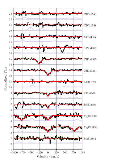
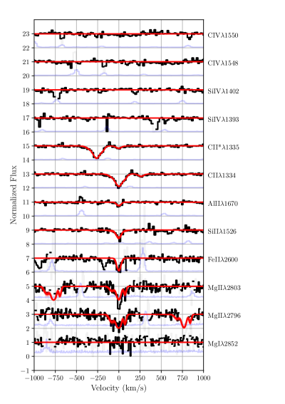
Figure 1 displays the spectral data from FIRE (left) and XShooter (Right) with the fitted model profiles overlaid in red. The model is the same for both panels; the only difference is in the convolution profile of the line spread function applied to data from each instrument. A randomly chosen sample of 75 models from the posterior distribution is plotted, making the width of the red curve a projection of model uncertainty onto the basis of the data. Associated fit parameters are listed in Table 1, reported as median values, with associated 5% and 95% confidence intervals of the posterior distributions. For undetected ions we report a 95% upper bound.

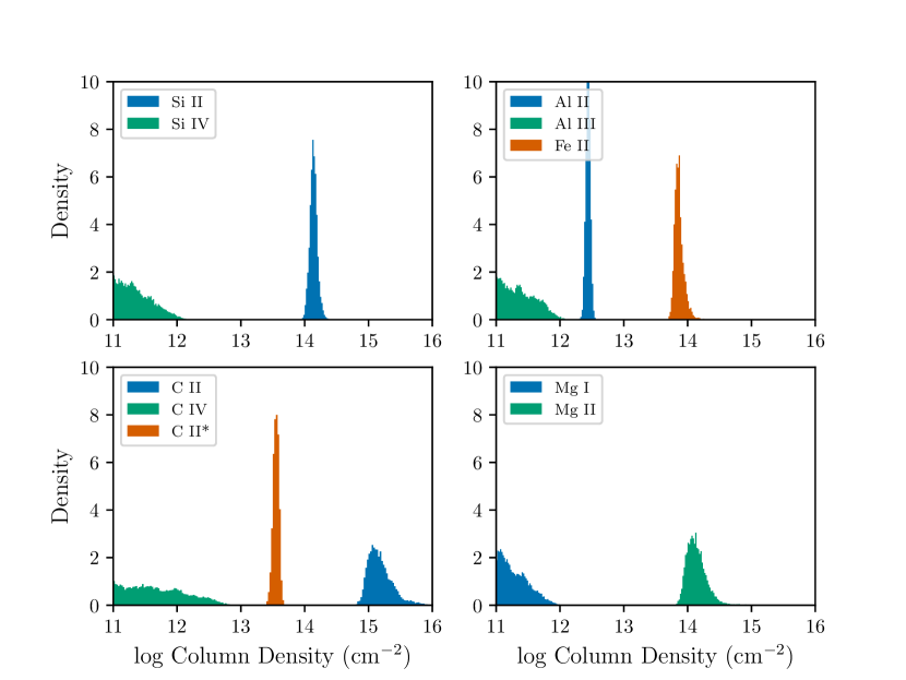
Our preferred model incorporates three absorption components: one strong line at $z=6.84329$, and weaker flanking components at $\Delta v=-73$ km s^-1 and $+76$ km s^-1. All three have best-fit $T\sim 7000-10000$ K and turbulent $b_{turb}\sim 25$ km s^-1. These three components spanning 150 km s^-1 are needed to fit broadened C II and Mg II profiles that are well-resolved (spaning three resolution elements of the spectrograph). The three-component model fits 26 independent parameters, achieving a reduced $\chi^{2}_{\nu}=0.94$ per degree of freedom. The full posterior parameter distributions are shown in Figure 2. For C II, Mg II, and Si II in this figure we show the summed total $N$ of the three absorption components.

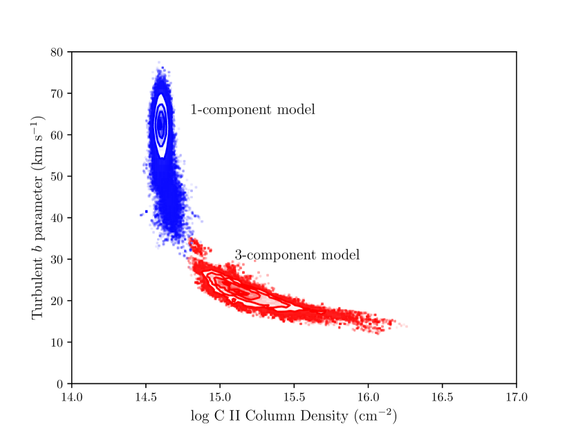
It is possible to achieve a similar quality of fit ($\chi_{\nu}=1.06$ per degree of freedom) using a one-component model with just 14 fit parameters, which would seem attractive because of simplicity. However this model requires a large turbulent broadening ($b_{t}=62$ km s^-1) driven by the need to span the resolved width of the C II and Mg II profiles. Figure 3 illustrates this effect by plotting contours of the 2D $N_{\rm CII}-b$ space explored by the MCMC walker, with blue contours tracing the one-component fit.

Although the one-component fit yields a narrower marginal distribution in C II column density and might therefore seem a “better” fit, this is only possible if $55<b<70$ km s^-1. Such extremely broad systems have not been obseved in metal absorbers at lower redshift, and even at $z>6$ the majority of O I and C II lines observed with HIRES exhibit low temperatures and quiescent kinematics (Becker et al., 2011; Cooper et al., 2019). We therefore disfavor the one-component model on physical grounds and concentrate on the three-component model for remaining analysis.

Figure 4: Detailed profile of the C II$\lambda$1334.5Å and C II*$\lambda$1335.7Å lines, without normalization by the continuum fit. Red curves indicate the continuum+absorption model for 100 random draws of the MCMC posterior.

Figure 5: Relative abundance of C, Si, Al and Mg relative to Fe, derived from singly ionized species of each element with no ionization correction applied. The new $z=6.84$ measurement is illustrated with a black star; literature measurements are indicated from lower-redshift quasar absorption line systems (Becker et al., 2012; Cooke et al., 2011; Dessauges-Zavadsky et al., 2003). The Solar scale is taken from Asplund et al. (2009). The offset histograms to the right of each panel show the abundance distribution of metal-poor stars in the Milky Way’s halo and in local dwarf galaxies (Abohalima & Frebel, 2018). We do not see evidence at $z=6.84$ for modified yields as might be expected for Population III stars or an evolving IMF. There is also no evidence for a change in the [$\alpha$/Fe] ratio as measured with C, Si and Mg, even though the Hubble time is just 794 Myr.

In the favored model, C II and Mg II arise in mildly saturated components that are individually unresolved by FIRE, but the overall complex contains discrete substructures whose kinematic motions are resolved. For C II, this leads to a high-end tail in the column density distribution that can reach as high as $10^{16}$ cm^-2 (Figures 2 and 3), but is concentrated between $10^{14.75}-10^{15.50}$ for $10<b<25$ km s^-1, which is more typical of metal absorbers at lower redshift.

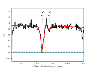
We obtain a highly significant detection and measure precise column density for the C II* excited state fine structure line, having verified that the absorption (which is visualized more clearly in Figure 4, along with the local continuum fit) is not from interloping systems at other redshift. This line is detected in many DLAs at lower redshift; it is sensitive to local heating in the neutral phase of interstellar gas, and will be discussed in depth below.

Figure 6: Ratio of triply-ionized to singly-ionized column density for C and Si, with increasing degree of ionization toward the upper right. The posterior distribution for the $z=6.84$ absorber in ULAS J1342 is shown in the contour/scatter distribution at lower left. Selected samples from the literature are shown with colored points as labeled in the legend and referenced in the text. This system has the strongest ionization limits yet observed, because of strong detections for C II and Si II  but sensitive upper limits on C IV  and Si IV. Some high-$N_{\rm HI}$ but metal-poor DLAs at lower redshift may overlap if more sensitive data are obtained.

Remarkably, we do not detect absorption from triply ionized species of any element — the upper limits on C IV are nearly 2 dex below the measured C II column. Unfortunately we cannot observe C III ($\lambda 977$Å) or Si III ($\lambda 1206$Å) because of Gunn-Petersen blanketing in the Ly $\alpha$ forest. The presence of singly-ionized species (and non-detection of Mg I) suggests that this gas is exposed to radiation in the $E=0.5-1.0$ Ryd band, but that the radiation field at harder energies (dominated by AGN) is weak compared to what is seen at lower redshifts.

4.2 Relative Abundances

Measurements of absolute heavy element abundances on a hydrogen scale are impossible at $z>6$ because H I  is blended in the forest. However our detection of Fe II enables evaluation of relative heavy element abundances compared to the Solar pattern, which we normalize to the photospheric scale of Asplund et al. (2009). This constitutes the earliest direct measurement of any abundance, well within the first Gyr of cosmic history.

Motivated by our non-detection of doubly- or triply-ionized species, we follow the approach used for abundance analysis of Damped Lyman Alpha (DLA) absorbers at low redshift, assuming all gas is in the neutral phase, and no ionization correction is required (Wolfe et al., 2005). This assumption is self-consistent if the absolute abundance is below roughly [Fe/H]$\leq-2.0$; at these levels the H I column density implied by our C II and Si II measurements would exceed $N_{\rm HI}=10^{20.3}$ cm^-2 (the canonical DLA $N_{\rm HI}$), using the Solar abundance scale of Asplund et al. (2009). We further verified with cloudy calculations that for $N_{\rm HI}=10^{21}$ cm^-2, the ionization fractions of our observed transitions were all $\gtrsim 95$%, and abundance corrections were at the 0.01-0.02 dex level, far below random observational errors. If the absolute abundance is higher, then the H I column would be lower and an ionization correction may be required. We revisit this assumption in Section 4.3.

Table 2: Relative Abundance Measurements

Ratio	Median Value
[C/Fe]	$+0.36~{}[+0.24,+0.54]$
[Si/Fe]	$+0.26~{}[+0.19,+0.33]$
[Al/Fe]	$-0.37~{}[-0.45,-0.31]$
[Mg/Fe]	$+0.16~{}[+0.03,+0.30]$

Note. — Bracketed values encompass 16/84% of MCMC posterior distributions.

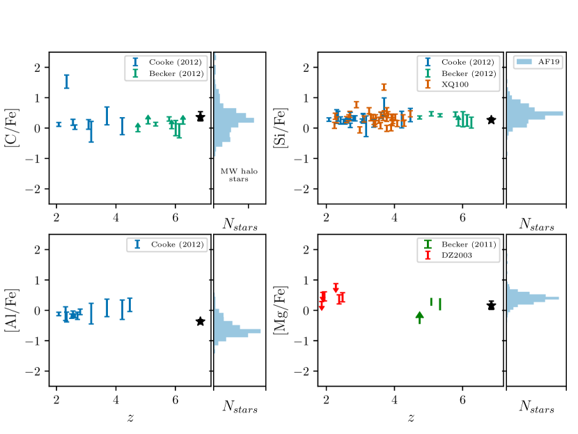
Figure 5 shows the abundances of C, Si, Al and Mg relative to Fe. In each panel, we show abundances of the same element measured in other quasar absorption systems at lower redshifts (Becker et al., 2012; Cooke et al., 2011; Dessauges-Zavadsky et al., 2003), and also distributions for metal-poor stars in the Milky Way and nearby dwarf galaxies taken from the JINAbase literature compilation (Abohalima & Frebel, 2018). The $z=6.84$ absorption system is shown as a black star at right.

We do not see any clear evidence at $z=6.84$ of anomalous relative abundances that would suggest an evolution in heavy element yield patterns. In particular we do not observe evidence of a large C enhancement, as has been seen in some metal-poor halo stars and suggested as a signature of early metal enrichment (Frebel et al., 2005).

There is tentative evidence of a sub-solar Al abundance, which is intriguing because metal-poor DLAs at $2<z<4$ appear to follow the Solar pattern, but metal-poor local stars are also centered around [Al/Fe]$\sim-0.5$. Some metal-pool LLS at $2<z<3.5$ also appear to be deficient in Al (Glidden et al., 2016).

Perhaps the most interesting implication is that the [$\alpha$/Fe] ratio as probed by C, Si, and Mg does not show any marked enhancement in a cross-section selected gas cloud just $\sim 800$ Myr after the Big Bang. This means that Fe production must already be robust even though enrichment from Type Ia supernovae is unlikely to be fully underway (Matteucci & Recchi, 2001). Similar findings have been extensively documented in broad line regions of $z>6.5$ quasars (De Rosa et al., 2014; Onoue et al., 2020; Mazzucchelli et al., 2017; Barth et al., 2003; Dietrich et al., 2003). However absorber-derived abundances should be more representative of the general IGM/CGM than an AGN broad-line region, and they should also be less susceptible to systematic offsets caused by local ionizing sources. This extends the findings of Becker et al. (2012) at $z=6.1$ (922 Myr after the Big Bang) now to $z=6.84$ (794 Myr). The absence of strong evidence for unusual yield patterns suggests that early generations of Population II-like stars were forming in this neighborhood by $z\gtrsim 10$.

4.3 Ion Ratios

Ratios of singly- to triply-ionized species of the same element encode information about ionization, independent of uncertainty of nucleosynthetic yields or relative abundances. A striking aspect of the $z=6.84$ absorber is its very strong C II and Si II with sensitive non-detections of C IV and Si IV. Undetected high-ionization-potential lines yield only a one-sided constraint on ionization. However unlike systems where both C II and C IV are detected, these systems have no ambiguity about whether gas giving rise to absorption from different species occupies a different phase region in the temperature-density plane.

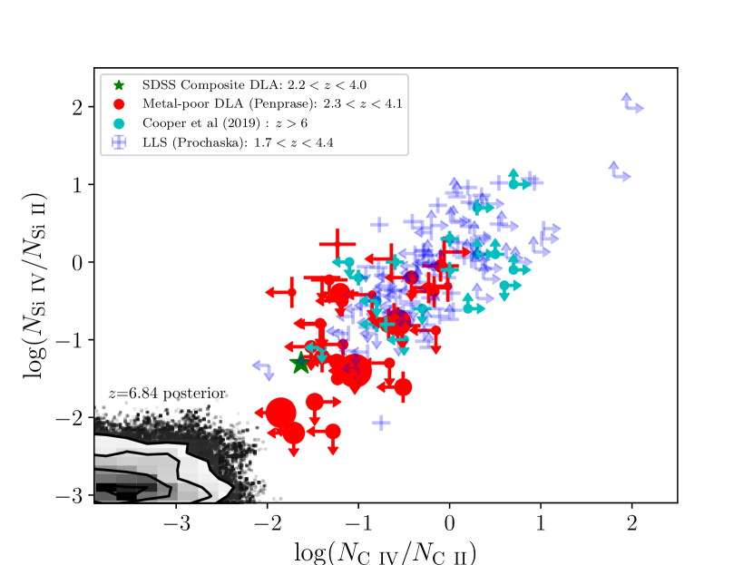
In Figure 6, we show with gray 2D contours the allowed posterior region in the $N_{\rm CIV}/N_{\rm CII}$ vs. $N_{\rm SiIV}/N_{\rm SiII}$ plane for the $z=6.84$ absorber. The ratios are configured such that more highly ionized systems appear at the upper right of the plot. The allowed region for the $z=6.84$ absorber is at the extreme bottom left—in fact it extends off the corner of the plot, because of non-detections in C IV and Si IV.

We estimate with 95% confidence that $N_{\rm SiII}:N_{\rm SiIV}>28:1$ and $N_{\rm CII}:N_{\rm CIV}>130:1$; the posterior is centered around a region of much lower ionization, near $N_{\rm CII}:N_{\rm CIV}=1200:1$.

To contextualize this result, we show the ratio derived from other selected samples in the literature that list $N$ for all four ions, at both low and high redshift. Light blue points indicate the locus of Lyman Limit Systems at $z\sim 3$ (Prochaska et al., 2015); red points correspond to a Penprase et al. (2010) sample of metal-poor DLAs at similar redshift. For the DLA sample, the point size scales with H I column density. A green star shows the value for a composite spectrum of DLAs stacked from the SDSS (Khare et al., 2012).

The absorber studied here has the highest redshift, and also the lowest ionization ratios yet observed for carbon and silicon. This is especially true for the C IV/C II ratio, which has limits 1-2 dex below the values observed for many LLS and DLAs.

Several points are shown in cyan from Cooper et al. (2019), who measured a larger sample of low-ionization absorbers at high redshift. Many of these may also overlap with the system studied here, but they generally have two-sided upper limits on these ratios that are less sensitive. Better spectra could place them in the region measured for our absorber.

The large majority of LLS have well-bounded, unsaturated detections of all transitions, or else a detection of C IV and Si IV without any detection of C II or Si II, placing them firmly in the top right of the ionization plane. The ULAS J1342 absorber is qualitatively distinct from low redshift LLS in its ion ratios.

A portion of the Penprase et al. (2010) metal-poor DLAs could occupy the same ionization space as the $z=6.84$ absorber, if the true value of $N_{\rm CIV}$ for the Penprase systems is well below their measured upper limits (for non-detections) and the true value of $N_{\rm CII}$ is well above their lower limits (from saturation). This is consistent with the interpretation advanced in Cooper et al. (2019), where low-ionization absorbers at $z>6$ are early analogs of DLAs, except that all are younger and more metal-poor. The distinct space occupied by the high redshift system in this diagram is a consequence of slightly more sensitive upper limits on $N_{\rm CIV}$ and $N_{\rm SiIV}$, but significantly higher estimates of the column density for both low ionization species.

5 Analysis of the Observed Neutral Medium

At low to intermediate redshifts, DLAs are often interpreted as an absorption-line manifestation of the multi-phase interstellar medium described by McKee & Ostriker (1977) and further refined by Wolfire et al. (1995). At $z=6.84$ it is unlikely that interstellar matter would be gathered into a large, dynamically cold disk. However the concept of multiple phases in pressure equilibrium and governed by heating and cooling processes is instructive.

In this paradigm, absorption line measurements can trace four different states of interstellar matter (Draine, 2011). First, a Cold Neutral Medium (CNM) with $T\sim 100$K exists in filamentary structures with galactic volume filling factor of a few percent, but a substantial fraction of the baryonic mass. Second, a Warm Neutral Medium (WNM) with $T\sim 7000$ K and lower density occupies $\sim 20\%$ of the volume, often at the boundary between the widespread ISM and smaller CNM regions or molecular clouds. These two phases are rich in neutral atomic gas and produce the damped H I profiles used to classify DLAs. Third, a Warm Ionized Medium (WIM) with $T\sim 10-15,000$ K—similar to the temperatures inferred from our Voigt profile fits—and low neutral fraction fills much of the ISM and is seen in diffuse H$\alpha$, rotation measure of radio sources, and C IV absorption. These phases are all in pressure equilibrium with a fourth Coronal hot phase, made up of tenuous ($n\sim 10^{-3}$ cm^-3) ionized gas with $T-10^{5}-10^{7}$ K. The hot corona fills 30-70% of the Milky Way’s ISM, extends into the wider circumgalactic medium, and is seen chiefly in O VI, X-ray line absorption, or optically thin H I absorption against background continuum sources.

In nearly all DLAs at $z<6$, one sees evidence for all of these phases (Prochaska et al., 2003), as a single sightline can penetrate regions of CNM, WNM, WIM, and coronal absorption in a single galaxy. As Figure 6 hints, essentially every $z<6$ DLA with neutral (e.g. Mg I) or singly ionized (e.g. C II, Si II) metal lines from the CNM or WNM also exhibits ions from the WIM (C IV, Si IV) or even O VI (Fox et al., 2007) that could come from the hot phase. This follows naturally from the fact that absorption probability depends on covering factors or geometric cross-section (Stern et al., 2016). The ionized ISM and corona have higher filling factor than the CNM and WNM, and extend into the CGM. This explains why highly ionized species are always found in systems selected by DLA absorption at lower redshift, while the converse is not true.

In many absorbers at $z>6$ (Cooper et al., 2019), and most strikingly in the system studied here at $z=6.84$, randomly-intercepted metal absorbers appear to trace some combination of the WNM and CNM, but the WIM and hot coronal phase are either not present or they can no longer be traced by rest-UV metal absorption lines.

We speculate three possible explanations for the WIM’s disappearance:

1. The WIM does not exist, or has not been heated into equilibrium with the CNM and WNM. This interpretation seems unlikely because our detection of C II* implies some amount of local heating in the neutral medium. If this heating is driven by star formation and supernovae, the same processes would also naturally yield a hot phase. In the CGM, much of the heating is driven by ubiquitous gravitational processes.

2. The WIM phase exists but has not been enriched with heavy elements. This could affect the cooling properties of the ISM at early times.

3. Any photoionization of tenuous gas in the CGM is driven by a background radiation field with low ionization parameter and/or soft spectrum.

We evaluate these interpretations by developing a two-phase model of the neutral medium consistent with all absorption columns plus the observed heating implied by detection of C II*. We then examine the expected properties of an unseen interstellar or circumgalactic hot phase for comparison with observational constraints.

5.1 C II^∗ and Local Sources of Heating and Cooling

Detections of C II* require that some fraction of bound electrons in C⁺ have been excited from the ${}^{2}P_{1/2}$ to the ${}^{2}P_{3/2}$ state, at which point they radiate fine structure [C II] photons at $\lambda=158\mu$m. This highly efficient line dominates overall cooling of the ISM in the Milky Way and local galaxies, and is routinely observed at high redshift using ALMA.

The emission rate of [C II] 158$\mu$m radiation (per H atom) can be measured for C⁺ atoms whose ${}^{2}P_{3/2}$ abundance is measured via C II* absorption (Pottasch et al., 1979):

$$l_{c} = h\nu_{ul}A_{ul}N_{\rm CII*}/N_{\rm HI}$$ (1)

$$= 10^{-26.6}\left({{N_{\rm HI}}\over{10^{20.6}{~{}\rm cm}^{-2}}}\right)^{-1}{~{}\rm erg}~{}{\rm s}^{-1}~{}{\rm H}^{-1}.$$ (2)

In Equation (2) we have substituted our measured value for $N_{\rm CII*}$ from Table 1, and scaled to $N_{\rm HI}$$=10^{20.6}$. $A_{ul}=2.36\times 10^{-6}$ s^-1 is the coefficient for spontaneous decay through [C II] photon emission, and $h\nu=1.26\times 10^{-14}$ erg is the energy of that photon.

Wolfe et al. (2003) developed a framework for estimating the star formation surface density in DLAs where the C II* abundance can be measured. The premise behind this method is that the ${}^{2}P_{3/2}$ state must be populated by a combination of (a) radiative excitation from CMB photons and optical pumping, and (b) local sources of heating, most of which scale with the local star formation rate (SFR, hereafter $\dot{\psi}$, measured as a surface density in units of $M_{\odot}$ yr^-1 kpc^-2).

For a fixed SFR, the balance of local heating and cooling results in an emergent two-phase medium (Wolfire et al., 1995), as is seen in the Milky Way’s ISM. The phase diagram $P(n)$ reveals a small range of $n$ where two dynamically stable solutions (i.e. $dP/dn>0$) can co-exist at different density but the same pressure. These are conventionally associated with the WNM and CNM. Gas in these phases is in pressure, but not thermal equilibrium. As the SFR increases and heating is enhanced, the characteristic $n,T$ and $P$ of these stable solutions for the CNM and WNM increase accordingly.

The same heating/cooling balance calculations used to estimate $(n,T,P)$ for a given $\dot{\psi}$ also naturally yield a curve of [CII] emissivity versus density $l_{c}(n)$, since the 158 $\mu$m line must be accounted in any budget of ISM cooling. The emissivity varies with both metallicity and dust depletion, both of which are observable in DLAs.

This leads to the following iterative procedure to find the SFR surface density $\dot{\psi}$ in a DLA where C II* is detected:

1. Calculate observational bounds on $l_{c}$ using measurements of $N_{\rm CII*}$, an assumption for $N_{\rm HI}$, and Equation (1).

2. Specify an initial guess for $\dot{\psi}$, and generate a phase curve $P(n)$ for that balance of heating and cooling (described below).

3. From the phase curve, evaluate the characteristic stable densities of the two phase medium $n_{\rm WNM}$ and $n_{\rm CNM}$, for that choice of $\dot{\psi}$.

4. Using cooling estimates from the same calculation and additional estimates of photo-excitation of the ${}^{2}P_{3/2}$ state, extract a second model curve of [CII] emissivity versus density $l_{c}(n)$.

5. Evaluate the model emissivity curve ($l_{c}(n)$) at $n=n_{\rm WNM}$ and $n=n_{\rm CNM}$ found in Step 3. These are the two possible/stable values that $l_{c}$ could take for this choice of $\dot{\psi}$.

6. Compare the model $l_{c}(n_{\rm CNM})$ and $l_{c}(n_{\rm WNM})$ to the observed value from Step (1). If the model underpredicts (exceeds) the data, increase (decrease) the model’s $\dot{\psi}$ and repeat from (2) until convergence. In general, the WNM will match the data for higher values of $\dot{\psi}$ and lower $n$ than the CNM, because [C II] has a lower fractional contribution to the cooling budget in the WNM.

Using this method, Wolfe et al. (2003) calculated star formation surface densities for $\sim 30$ DLAs, with average values of $\dot{\psi}\sim 10^{-2.2}$ $M_{\odot}$ yr^-1 kpc^-2 if the absorption is from a CNM and $\dot{\psi}\sim 10^{-1.3}$ $M_{\odot}$ yr^-1 kpc^-2 for a WNM. For comparison, the Milky Way has $\dot{\psi}\sim 10^{-2.4}$ $M_{\odot}$ yr^-1 kpc^-2 (Kennicutt, 1998) and Lyman Break Galaxies have $>1$ $M_{\odot}$ yr^-1 kpc^-2 (Pettini et al., 2001).

Figure 7: Two-phase model for the neutral ISM at $z=6.84$, assuming the cosmic ray ionization rates from Wolfe et al. (2003). (a) Phase curve of pressure vs. density, for star formation densities as indicated in the legend. For each model, at the inflection pair in the $P/k$ curve, gas at two different densities can exist at the same pressure, leading to a two-phase medium provided $dP/dn>0$ for stability. For the red curve, a warm neutral medium (left branch) matches the derived [C II] emissivity, whereas a cold medium (right branch) matches for the blue curve. Panel (b) shows the associated temperature profiles, with starred points indicating the solution matching this absorber. Panel (c) indicates the (logarithmic) ionized fraction and Panel (d) the [C II] emissivity. Solutions occur at the density $n$ where these curves both intersect the observational constraint (indicated with a black dashed line) and yield a stable two-phase medium for that SFR. Note that the two starred solutions are not in pressure equilibrium with each other. Rather, the blue star represents a unique model where a CNM can produce the observed amount of C II*, and is in pressure equilibrium with a warm phase not seen in absorption. The red star represents a model where a WNM can produce the observed C II*absorption, and is in equilibrium with a CNM that is not intersected by the sightline.

5.2 cloudy Implementation of Two-Phase ISM Model

We have built a revised version of Wolfe’s two-phase model to examine heating and cooling in the neutral medium of our $z=6.84$ absorber. Using cloudy, we simulated a plane-parallel slab of $N_{\rm HI}$$=10^{20.6}$ cm^-2 illuminated externally by a metagalactic background radiation field. The external field’s normalization and spectral shape are specified as in Faucher-Giguère (2020) for the absorber redshift. We also added a blackbody spectrum of CMB radiation for $z=6.84$, as the CMB becomes a non-negligible source of photo-excitation of the C II* fine structure line at low density.

Although we included an external radiation environment, heating of the neutral medium is in fact dominated by local processes, with the following four main contributors, all of which scale with the SFR.

5.2.1 Photoelectric Heating of Dust Grains

Far-UV radiation (6-13.6 eV) from massive stars can eject photoelectrons from dust grains, heating the ambient medium via Coulomb interactions with surrounding electrons. This heating rate depends on both the local abundance of dust grains, and the strength of the FUV radiation field which is presumed to be $\propto\dot{\psi}$.

cloudy implements dust in its solution via the grains command, which inserts a mixture of graphite and silicate grains with size distribution appropriate to the Milky Way’s ISM. However our absorber’s dust abundance should be much lower than that of the Galaxy on account of its lower heavy element abundances. We assumed that the grain abundance scales linearly with gas phase metallicity, and then applied a modest correction for depletion.

For the model specification of $N_{\rm HI}$$=10^{20.6}$, a gas phase metal abundance of [Si/H]$=-2.2$ yields the observed $N_{\rm SiII}$, and we scale dust grains downward by the same factor. An additional downward correction of $-0.43$ dex is made to the grain abundance to account for possible depletion as traced by the [Fe/Si]$=-0.2$ ratio, following Equation 7 of Wolfe et al. (2003).

We deviated slightly from Wolfe’s method of modeling the interstellar radiation field. Their analysis scales dust heating with $G_{0}$, the mean local intensity between 6-13.6 eV (Habing, 1968), correcting for different (and unknown) DLA geometries. Here we use cloudy’s Table ISM command to insert a spectral model of the ISM radiation field from Black (1987). We renormalize the local radiation field’s intensity according to the selected star formation rate, $(\dot{\psi}/10^{-2.4}~{}{\rm M}_{\odot}{\rm yr}^{-1}{\rm kpc}^{-2}$), where the normalization factor is again matched to the star formation surface density of the Milky Way.

5.2.2 Cosmic Ray Heating

We introduce cosmic ray heating using the cosmic rays background command in cloudy. Estimates of the Milky Way’s primary cosmic ray ionization rate are evolving and have been updated since publication of Wolfe et al. (2003). We therefore perform two calculations of the SFR. The first is for consistency with Wolfe et al. (2003), and assumes a primary cosmic ray ionization rate of $1.8\times 10^{-17}$ s^-1, as in Wolfire et al. (1995). The second is the default now assumed for cloudy, with a primary CR ionization rate of $2\times 10^{-16}$ s^-1 (Indriolo et al., 2007; Indriolo & McCall, 2012)—over $10\times$ higher.

As with the interstellar FUV radiation field, we scale the cosmic ray ionization rate in units of star formation rate relative to the Milky Way since supernovae are thought to be a significant source of galactic primary cosmic rays.

Because the Indriolo et al. (2007) ionization rates are higher than those of (Wolfire et al., 1995), they generate more heating per unit of SFR. Consequently these models require lower SFR to achieve levels of C II* detected in high-redshift DLAs. Cosmic ray heating is a non-negligible—and often the dominant—fraction of the total heating budget in all of the equilibrium solutions found below.

5.2.3 X-Rays, $H_{2}$, and Photoionization

Heating from X-rays and photoionization of C I is treated self-consistently by cloudy, given the input radiation spectrum from local sources and the extragalactic background.

Heating from collisional de-excitation of vibrational energy from molecular H₂ is also included self-consistently by cloudy. Our simulations show that this term becomes important at high densities, above $\gtrsim 1000$ cm^-3.

5.2.4 Grid Parameters

We executed a grid of models with the above heating inputs at fixed points in density and temperature, ranging from $-2<n<+4$ cm^-3 in steps of 0.2 dex, and $1<\log T<5$ K in steps of 0.2 dex. For each choice of $(n,T)$, we had cloudy output the total heating and cooling rates, the pressure, the H I ionization fraction, and the total [C II] 158 $\mu$m emissivity (from both cooling and photo-excitation). To fix the grid temperature in each run by fiat, we turned off cloudy’s temperature stopping criterion, and instead set the stopping condition to match $N_{\rm HI}$.

For each value of $n$, there is a single value of $T$ for which the heating and cooling rates balance. For each grid step in $n$ we interpolated the output heating and cooling curves to determine this equilibrium $T$, reducing these state variables to a one-dimensional locus.

Table 3: Two-Phase ISM Model Parameters

		CLOUDY cosmic rays		Wolfe et al. (2003) cosmic rays
		WNM	CNM	WNM	CNM	Observed
$\log\dot{\psi}$	(M⊙ yr-1 kpc-2)	-1.97	-2.55	-1.03	-1.95
$\log n$	(cm-3)	1.26	2.82	1.32	2.08
$\log T$	(K)	3.8	1.66	3.8	2.0
$P/k$	(cm-3 K)	5.18	4.53	5.18	4.13
$N_{\rm CI}$	(cm-2)	11.68	13.34	11.12	12.44	$<$12.85
$N_{\rm CII}$	(cm-2)	14.99	14.98	15.12	14.98	15.09 [14.86,15.54]
$N_{\rm CIV}$	(cm-2)	3.44	$\cdots$	9.37	$\cdots$	$<$12.50
$N_{\rm CII*}$	(cm-2)	13.81	13.73	13.76	13.96	13.55 [13.47,13.62]
$N_{\rm SiII}$	(cm-2)	14.15	14.14	14.17	14.14	14.09 [14.00,14.20]
$N_{\rm SiIV}$	(cm-2)	7.78	$\cdots$	9.60	$\cdots$	$<$11.85
$N_{\rm MgI}$	(cm-2)	11.52	12.69	11.12	11.88	$<$11.72
$N_{\rm MgII}$	(cm-2)	14.14	14.12	14.15	14.14	13.90 [13.73,14.20]
$N_{\rm FeII}$	(cm-2)	13.85	13.85	13.87	13.85	13.86 [13.77,14.01]
$N_{\rm AlII}$	(cm-2)	12.47	12.47	12.48	12.46	12.44 [12.38,12.50]
$N_{\rm AlIII}$	(cm-2)	10.11	8.80	10.86	9.73	$<$11.82

5.3 Model Results

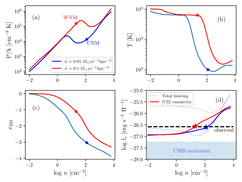
Figure 7(a) shows the resulting phase curves of $P(n)/k$, as well as (b) $T(n)$ and (c) the ionization fraction $x(n)$, for the cosmic ray normalization used by Wolfe et al. (2003). A stable two-phase medium exists at the inflection of each $P(n)$ curve, between the local maximum $P_{max}$ and minimum $P_{min}$. In this region the density may take on any value, provided $dP/dn>0$ for stability. By convention (Wolfire et al., 1995) we calculate the WNM and CNM densities at the geometric mean between the maximum and minimum pressure $P_{eq}=\sqrt{P_{min}P_{max}}$, for each model (i.e. red or blue curves)

In Panel (d), we show the total heating rate (dashed line), and the [C II] 158 $\mu$m emission rate (i.e. the model $l_{c}$) per H atom (solid line). The observed $l_{c}$ is shown with a horizontal line, because the density $n$ is not specified by observations and must be inferred by model comparison. The intersection of the dashed black data line and the solid red/blue model lines in panel (d) correspond to $(n,P,T)$ triplets for a given star formation rate, where the neutral ISM is in two phase pressure equilibrium and the [C II] emission matches observations. The model parameters corresponding to these solutions are shown in Table 3.

On each curve, we have highlighted with a starred point the CNM or WNM solution that matches the inferred C II cooling rate, $l_{c}$. Because this match occurs at a different value of $\dot{\psi}$ for the CNM and WNM, the two solutions are shown with blue and red curves, respectively. The CNM solution converges on $n=120$ cm^-3 ($\log n=2.08$), and $T=100$ K ($\log T=2.0$).

The star formation surface density that leads to a matching CNM in this model is $\dot{\psi}=10^{-1.95}~{}{\rm M}_{\odot}~{}{\rm yr}^{-1}~{}{\rm kpc}^{-2}$, about $3\times$ higher than the Milky Way but lower than starburst galaxies.

The corresponding WNM solution has $n=21$ cm^-3 ($\log n=1.32$), $T=6300$ K ($\log T=3.8$), and $\dot{\psi}=10^{-1.03}~{}{\rm M}_{\odot}~{}{\rm yr}^{-1}~{}{\rm kpc}^{-2})$, roughly $10\times$ higher than the CNM solution and $30\times$ higher than the Milky Way.

For comparison we also show in Table 2 the solution space for the alternate cosmic ray heating model of Indriolo et al. (2007) as implemented in cloudy. Recall that this model has $10\times$ higher CR ionization than Wolfe’s for a given SFR. Stable solutions exist at lower SFR, since these solutions exist where heating and cooling balance and the same CR heating is achieved at lower SFR.

For the WNM, the scaling is simple: at $10\times$ lower SFR, the model converges on the same $(n,T,P)$ triplet as the WNM for the Wolfe et al. (2003) model. In contrast, the Indriolo CNM solution occurs at only $3\times$ lower SFR, but much higher density, and lower $T$.

5.4 Comparison with Absorption Columns

The cloudy models developed above produce column density predictions for all species through the slab, which may be compared against the observed values. These are shown at the bottom of Table 2, with the Voigt profile model parameters of Table 1 reproduced in the rightmost column for ease of comparison. Recall that these solutions assume [Fe/H]=-2.2 for the gas phase, $N_{\rm HI}$=$10^{20.6}$, and modest dust depletion as in Equation 7 of Wolfe et al. (2003). Also, we have applied slight relative abundance corrections to map the overall [Fe/H] into each individual element, using the values from Table 2.

For both models of cosmic ray heating, the WNM solution predicts column densities consistent with the quoted observational confidence limits, in every ion. The inferred temperature of $T=6300$ K is also broadly consistent with the $b$ parameters of our best-fit Voigt profiles, although the line widths are smaller than our spectral resolution and hence have large uncertainty.

The CNM absorption columns largely agree for singly ionized species and above, but show tension between the models and observations for the neutral species Mg I and C I. The disagreement is minor and shown with blue text in Table 2 for the Wolfe et al. (2003) model of cosmic ray heating, but the disagreement is large for the Indriolo et al. (2007) cosmic ray model, and is shown with red text.

This tension arises because the cosmic ray heating becomes so efficient that very little star formation is needed to maintain thermal balance at high gas densities. With few massive stars, the FUV radiation field at 0.5-0.8 Rydbergs (the ionization energies of C I and Mg I) is correspondingly weak, resulting in a higher neutral fraction and correspondingly larger column densities that should be detected for these species. Our non-detections of Mg I and C I disfavor solutions where the absorption arises from a CNM with efficient CR heating.

The observations are fully consistent with models of a two-phase medium where the absorption arises in a WNM of abundance [Fe/H]=-2.2, SFR surface density modestly higher than the Milky Way, $T\sim 6000$ K, and only minor levels of dust depletion. CNM solutions with higher density and lower temperature are marginally consistent with the data, but only if the coupling between star formation and cosmic ray heating is less efficient than indicated by the most recent estimates for the Milky Way.

5.5 Effect of Varying $N_{\rm HI}$

The cloudy models developed above all assume $N_{\rm HI}$$=10^{20.6}$ cm^-2, but this value cannot be constrained by the spectral data. Here we examine whether the conclusions reached above are robust if the value of $N_{\rm HI}$ changes.

Suppose that $N_{\rm HI}$ increases by one dex. By Equation 1 the [C II] emission rate per H atom will also decrease by 1 dex, since there are 10$\times$ more H atoms per C atom. In Figure 7(d), this corresponds to a reduction of horizontal black dashed line, toward the region where CMB excitation becomes a factor in generating [C II] emissivity.

However the CMB excitation rate per H atom is also directly proportional to the carbon abundance, and therefore inversely proportional to $N_{\rm HI}$. So, even though $l_{c}$ decreases as $N_{\rm HI}$ grows, the CMB excitation rate decreases by the same amount. Put another way, the observed C II* column requires more excitation of the ${}^{2}P_{3/2}$ state than the CMB alone can provide even at $z=6.84$, no matter what value is chosen for $N_{\rm HI}$.

The total heating rate does not change as $N_{\rm HI}$ is varied, because heating is dominated by cosmic rays, which scale with SFR but not $N_{\rm HI}$. However as $N_{\rm HI}$ increases the heating rate per H atom will decrease in direct proportion, causing the dotted red/blue lines to move downward in Figure 7(d) by the same amount as the CMB excitation.

The total cooling rate is dominated by [C II] fine structure emission and is therefore constrained by the directly observed C II* column, rather than $N_{\rm HI}$. Again, because the emissivity (solid) curves in Figure 7(d) are [C II] emissivity per H atom, an increase in $N_{\rm HI}$ lowers these curves by an identical amount.

Synthesizing all of these factors: varying the H I column density shifts all of the curves in 7(d) up or down by the same amount, so the intersection of the model and observed [C II] emissivity (starred points) falls at the same value of $\log n$, and therefore corresponds to the same value for $T,P$ and the WNM and CNM solutions. There may be subtle effects if dust depletion patterns change with metallicity, or if collisional de-excitation of ro-vibrational transitions of H₂ begin to manifest at high $n$ in the CNM. However the basic features of the model, including enhanced excitation above the CMB baseline, and a stable two-phase solution at similar points of $(n,T,P)$, do not change with $N_{\rm HI}$ so long as it remains in the damped Lya or neutral state.

5.6 Order-of-Magnitude Estimates of [C II] Luminosity

The C II* column density is a direct measure of the surface density of atoms in the excited fine structure state. Together with the spontaneous decay rate, this can be used to project the [C II] 158 $\mu$m luminosity, given strong assumptions about geometry:

$$L_{[\rm CII]}=(h\nu_{ul}A_{ul}N_{\rm CII*})\times 4\pi S_{\rm[CII]}.$$ (3)

Here, $S_{\rm[CII]}$ is the integrated surface area of the [C II] emitting regions, which is model dependent. If we assume a [C II] half-light radius $r_{e}\sim 3$ kpc measured for $z\sim 6.5$ galaxies (Smit et al., 2018), and set $S_{\rm[CII]}=\pi r_{e}^{2}$, this yields a total estimated luminosity of

$$L_{\rm[CII]}\sim 10^{6.3}~{}~{}L_{\odot}$$ (4)

This estimate is highly speculative, but only partly because of the strong assumption on the half-light radius. Equally important, the absorption properties are slightly more consistent with a WNM (which has a larger volume and covering factor), yet for many galaxies the total [C II] emission is dominated by CNM gas in pressure equilibrium that is simply missed by the quasar absorption path. If the emitting region covers only a small fraction of the half light radius, then Equation 4 could overestimate the [C II] luminosity. However if the absorbing gas traces a WNM that is accompanied by stronger emission from the CNM, then Equation 4 would underestimate $L_{\rm[CII]}$.

As a separate consistency check, one can start instead with our estimates of the SFR surface density $\dot{\psi}$, calculate a total SFR integrated over the galaxy, and then use empirical or model correlations between total SFR and $L_{\rm[CII]}$ to estimate the 158 $\mu$m luminosity.

If we exclude the CNM model with cloudy’s default cosmic ray ionization (because of tension with C I and Mg I), the other models all have $\dot{\psi}\sim 0.01-0.1$ M_⊙ yr^-1 kpc^-2. Again combining this with the [C II] half-light radius $r\sim 3$ kpc (Smit et al., 2018), one derives a total star formation rate of order $0.3-2.0M_{\odot}$ yr^-1. Comparing to the [C II]-SFR correlations modeled by Lagache et al. (2018, Equation 10), we estimate:

$$L_{\rm[CII]}=10^{6.13}-10^{6.89}L_{\odot}$$ (5)

For EoR galaxies with $\log({\rm SFR})\sim 0$, Finlator et al. (2018) estimate stellar mass of $\log M_{*}\sim 8.5$ M_⊙.

These calculations, while crudely consistent, are meant to be heuristic guides rather than precise measurements. They demonstrate that absorption selection does uncover systems that are locally heated, yet produce quotidian [C II] luminosities and stellar population properties, much less extreme than the galaxies of high SFR or metallicity observed at high redshift (Neeleman et al., 2019, 2020). Such systems are predicted by numerical simulations but largely missed in all but the deepest flux-limited blind galaxy surveys.

6 Non-Detection of Warm Ionized Gas

6.1 No detection of metals in an ionized ISM

Multiphase models of the Milky Way’s ISM include a WIM in pressure equilibrium with the WNM; this WIM is traced in low surface-brightness H$\alpha$ emission (Haffner et al., 2003), rotation measures of radio sources (Taylor & Cordes, 1993), and in C IV absorption against the spectra of hot stars (Savage et al., 1997; Sembach et al., 2000). It is diffused through a large fraction of the Milky Way’s ISM volume with scale height of 1-3 kpc above the disk.

Warm ionized (C IV) and hot (O VI) gas have also both been studied in low-redshift DLAs; they are not precisely coincident in velocity space with the neutral medium that produces low-ionization lines (Fox et al., 2007). The hot O VI shows broad absorption widths and is consistent with a collisionally ionized gas at $T\approx 300,000$ K. The C IV absorption is slightly narrower and could be associated with either collisionally ionized gas at $T=100,000$ K where the C IV collisional fraction peaks, or at slightly lower $T$ with enhancement from photoionization. However standard thermal equilibrium assumptions are not always justified for the warm C IV gas. It can become unstable to cooling, yet during this cooling it can experience large departures from ionization equilibrium, such that the C IV fraction remains high as the gas cools to stability at $T=10,000$ K (Oppenheimer & Schaye, 2013).

In our multiphase model of the $z=6.84$ absorber, gas at the peak C IV ionization temperature of $T=10^{5}$ K would be in pressure equilibrium with the WNM ($P/k\sim 10^{5.2}$ cm^-3 K) if it has density $n=10^{-0.2}=0.6$ cm^-3. We ran simple cloudy calculations with these input $(n,T)$, and the WNM model values in Table 2 for the SFR $\dot{\psi}$, cloudy-default cosmic ray heating, including local+extragalactic background radiation fields. Because $N_{\rm HI}$ is not known and the ionized gas may be optically thin at the Lyman limit, we set the stopping criterion according to cloud thickness rather than $N_{\rm HI}$, using 1 kpc as a reference value.

With these inputs, if we assume the same value of [Fe/H]$=-2.2$ that was calculated for the WNM and CNM models, cloudy calculates a WIM ionized fraction of $\log x=-4.8$, and column densities:

$$N_{\rm HI} = 10^{16.51}\left({{\Delta L}\over{1~{}{\rm kpc}}}\right)$$ (6)

$$N_{\rm CIV} = 10^{14.57}\left({{\Delta L}\over{1~{}{\rm kpc}}}\right)$$ (7)

$$N_{\rm SiIV} = 10^{13.41}\left({{\Delta L}\over{1~{}{\rm kpc}}}\right).$$ (8)

While this value for H I is plausible, the predicted C IV column exceeds our observational bounds by 2.1 dex, and the Si IV limits by 1.6 dex.

To bring this WIM model C IV column into alignment with measurements, either its length scale must be reduced by a factor of $10^{-2.1}$ to $\sim 8$ pc, or the heavy element abundance must be reduced by 2.1 dex to [C/H]$<-4.2$ (95% confidence). For reference, the cloud depth required to reach DLA column densities for the WNM cloudy model (i.e. Table 2) is $\sim 20$ pc. If the WIM is enriched to the same abundance as the WNM, then it is over a $2-3\times$ smaller length scale and therefore its metals cannot be considered widely mixed into the ISM. Alternatively, any heavy elements mixed spatially into in the WIM on kpc or larger scales must be at $\sim 100\times$ lower abundance than the neutral medium where stars form. In some ways this represents an inversion of the prevailing paradigm of ISM and CGM absorption, where small neutral condensates are embedded in an ionized medium occupying a larger fraction of the volume (Stern et al., 2016). We are not arguing here that the ionized phase does not exists, only that it may not yet manifest in metal absorption because of low enrichment.

Figure 8: Corner plot of posterior distributions for the 5-parameter model discussed in Section 6.2. The narrow line in the $N_{\rm HI}$ vs. [Fe/H] plot traces out abundance values for a neutral medium, and the marginalized posterior of $N_{\rm HI}$ illustrates how DLA-like column densities are favored by the measured ratios of metal ions. The non-detection of C IV requires a weak ionization parameter $U$. A large break is required at the Lyman limit ($\tau_{\rm HI}$), so that there are enough $E<13.6$ eV photons to ionize Mg I, but few photons to produce C IV and Si IV. At the large H I columns that are favored, the system is self-shielded from hard-UV photons, so an unusually soft ionizing spectrum is not necessarily required.

A WIM with this $(n,T)$ combination and abundances is not in thermal equilibrium. The cloudy-calculated cooling rate exceeds the heating rate, meaning that C IV in a $T=10^{5}$ K WIM should cool on short timescales compared to the Hubble time. Non-equilibrium effects may enhance the C IV fraction relative to its photoionization equilibrium value as the cooling gas approaches $T\sim 10,000$ K from above.

The non-detections of C IV and Si IV imply that if this galaxy has a warm ionized component to its ISM as seen in the Milky Way and all lower redshift galaxies, then this WIM has not yet been enriched by heavy elements at $z=6.84$. Or, at least the degree of enrichment is substantially lower in abundance or occupies a smaller volume than nearby neutral regions.

6.2 No Detection of an Ionized Circumgalactic Medium

The multiphase models developed above are motivated by observations of interstellar matter in the Milky Way and other local galaxies, within their central, dynamically cold disk. Yet at lower redshift where host galaxies are more easily surveyed, most absorption systems and even many DLAs are located at large impact parameter ($10-100$ kpc) from the central galaxy and its associated ISM (Boettcher et al., 2020; Neeleman et al., 2017; Christensen et al., 2014; Tumlinson et al., 2017). If the $z=6.84$ absorption traces the extended tenuous CGM of a protogalaxy, a similar set of cloudy models can be used to constrain its ionization conditions.

Suppose we wish to generate a single-phase CGM absorption model consistent with strong detection of all low-ionization species, but sensitive non-detection of all conventional highly-ionized lines. Such a model requires some combination of a low ionization parameter $\log U$, self-shielding from a large H I column density, or a very soft spectral shape of the ionizing background radiation field.

To explore the trade space between these options, we ran a 5-dimensional grid of cloudy models varying the following parameters:

• $N_{\rm HI}$: The neutral H I column is not an observable, and must be treated as a model variable. We set a flat prior distribution in the logarithm with $19<\log N_{\rm HI}<21$ cm^-2.

• Ionization parameter: We varied $\log U$ from $-5$ to $-2$ with a flat prior in log space.

• Spectral slope: this parameter $\alpha$ sets the hardness of the UV background field $f_{\nu}\propto\nu^{\alpha}$ at energies above 1 Rydberg. We varied it between very hard values of $\alpha=0$ to very soft values of $\alpha=-6$, with flat prior.

• Spectral break $\tau_{\rm HI}$ at the Lyman edge: This is a feature of the UV background spectrum, specifying the strength of a decrement across the 1 Rydberg break. We sampled uniformly between $0<\tau_{\rm HI}<10$.

• Metallicity [Fe/H]: this parameter was varied between $-5<$[Fe/H]$<0$.

At each point on the grid, cloudy runs a simulation with stopping condition set on the specified H I column density, outputting column density predictions for every observed ion. We read these into a set of 5-d interpolation tables to calculate rapid column density predictions for any vector of model input parameters.

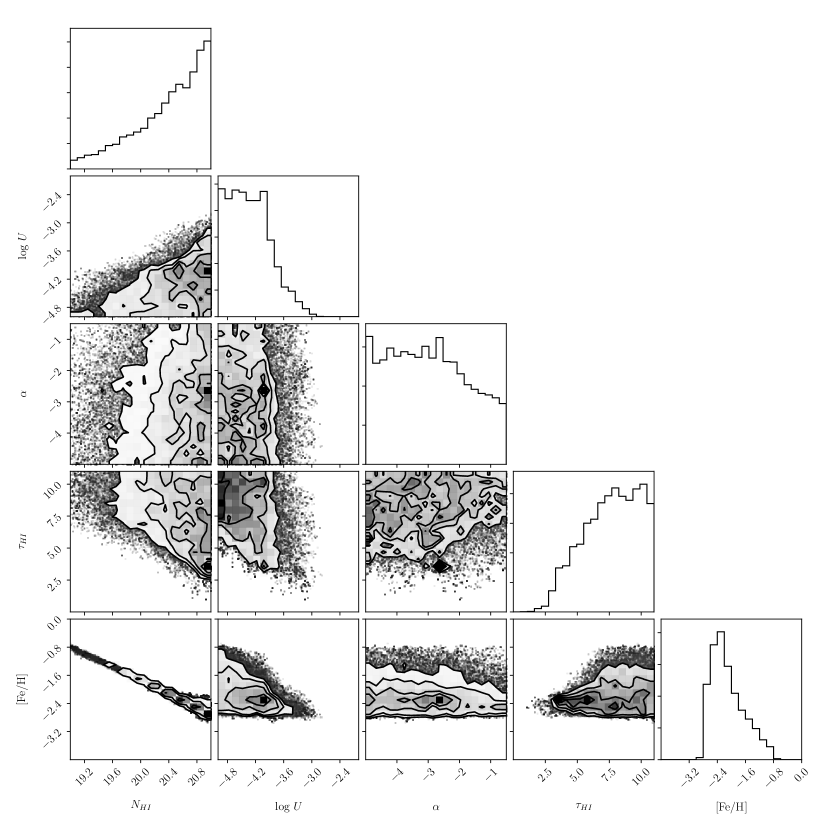
We explored the parameter space of these five variables with an emcee MCMC walker, calculating the likelihood at each step by comparing the model outputs with the measured column densities or upper limits for each ion, as described in Crighton et al. (2015). A corner plot of the output is shown in Figure 8. Because we do not measure $N_{\rm HI}$ and only have upper limits on C IV, Si IV, and Mg I, the MCMC walker does not converge on two-sided bounds for most model parameters. Instead, it delineates one-sided or diagonal bounds in each plane corresponding to allowed or disallowed regions of the parameter space.

A line of degeneracy in the [Fe/H] vs. $N_{\rm HI}$ posterior traces out the solution locus for a neutral medium with the observed metal-line columns, but the marginalized histogram of $N_{\rm HI}$ shows a clear preference for high H I column density values in the DLA range ($\log N_{\rm HI}>20.3$ by convention). The heavy element abundance is similar to the values used for the two-phase ISM model above (recall this model assumed $N_{\rm HI}$$=10^{20.6}$). Put another way, even when the walker explores a large solution space, the posterior ends up favoring a solution with H I column density characteristic of a DLA and abundance slightly below $1/100$ solar, rather than a more tenuous and ionized CGM.

The ionization parameter posterior favors very small values $U<10^{-4}$ which flow from the low C IV/C II and Si IV/Si II ratios. Importantly, for solutions with lower $N_{\rm HI}$ and higher [Fe/H] (which are more likely to require ionization corrections), the smallest values of $U$ are required to prevent overproduction of C IV.

Likewise, while all solutions require a strong break at 1 Rydberg of $\tau_{\rm HI}\gtrsim 3$, the lowest values of $N_{\rm HI}$ require the largest spectral breaks. For $N_{\rm HI}$$<10^{20}$, breaks of $\tau_{\rm HI}\gtrsim 6.5$ or more are needed. This is primarily to reproduce the large observed Mg II/Mg I ratio. Large breaks at 1 Rydberg ensure that there are enough soft-UV (0.56 Ryd) photons to ionize Mg I to Mg II, but not too many hard-UV photons that would ionize C II to C III (1.79 Ryd), or C III to C IV (3.52 Ryd).

This exercise demonstrates that even if we search a wide parameter space for single-phase solutions corresponding to more tenuous circumgalactic gas, an MCMC walker will still converge on models resembling a metal-poor but not chemically pristine DLA. In fact the inputs are very similar to the multiphase ISM model described earlier. Such systems could exist in the CGM of a protogalaxy, but would need to support some amount of local star formation to reproduce the observed C II*.

7 Discussion

The models outlined above shape our physical intuition about the environment of a star forming region randomly selected by intervening absorption cross section, when the Hubble time was just 794 Myr. This is among the first detailed characterizations of a non-extreme astrophysical environment in the epoch of reionization.

Strong absorption from singly ionized species such as C II, Si II, Al II, and Fe II requires a medium with a substantial H I neutral fraction, yet the lack of Mg I and C I implies some degree of ionization from the FUV radiation field of massive stars.

A confident detection of the C II* fine structure line constrains heating of the ISM by radiation and cosmic rays associated with those stellar populations and their associated supernovae. The inferred star formation surface density depends on whether the absorption traces a warm or cold neutral medium. However the derived SFR values are within a factor of three of what is seen in the Milky Way, and do not require exotic stellar populations, modifications to the interstellar radiation field or cosmic ray physics.

These two-phase ISM models—tuned to achieve pressure balance, heating/cooling equilibrium, and the [C II] emissivity—also correctly reproduce the observed column densities of all absorption species (except for CNM models with efficient cosmic ray heating, which overproduce Mg I). According to the cloudy outputs, neutral gas in this phase will never produce observable high-ionization absorption from C IV or Si IV.

The heavy element abundance depends upon one’s choice of $N_{\rm HI}$ (which is unconstrained by observations). For $N_{\rm HI}$$=10^{20.6}$ (a modest DLA), an abundance of [Fe/H]$=-2.2$ yields matching column densities; larger choices of $N_{\rm HI}$ lead to correspondingly smaller metallicity. This abundance is slightly lower than the median DLA metallicity at $z<4$, but not a strong outlier. Apparently rapid enrichment was already well underway in the neutral medium of this system, within its first few hundred Myr.

At lower redshifts, the C II and Si II which trace the optically thick neutral medium are always accompanied by strong C IV. This either arises in a warm-ionized phase of the ISM near the collisional ionization optimum for C IV ($T=10^{5}$ K), or else in lower density circumgalactic gas photoionized by the ambient background field. This high-ionization signature is completely absent in the system studied here, with stronger constraints than heave been measured for other DLAs at any redshift.

If a warm ionized phase exists in this system at $T\sim 10^{5}$ K, the non-detection of C IV places a degenerate constraint on its absorption pathlength and carbon abundance. For $\Delta L=1$ kpc (the scale height of the Milky Way’s WIM), one obtains [C/H]$<-4.6$ — indicating that metals produced in the neutral regions have not yet mixed throughout the ionized ISM.

The relative abundances of heavy elements do not show any noteworthy deviations from the Solar pattern, adding to the evidence that enrichment was driven by conventional Population II stars, rather than a top-heavy or Population III initial mass function.

It is possible to make order-of-magnitude estimates for the stellar mass and [C II] luminosity of the associated stellar population, under a strong assumption that the [C II] emissivity per kpc^-2 may be integrated over an area similar to the [C II] half light radius of other $z\sim 6.5$ objects (which is larger than the UV/optical half light radius). Using two different methodologies we estimate [C II] luminosity of $10^{6.1}-10^{6.9}L_{\odot}$. Integrating the SFR surface density over the [C II] half-light radius (assumed as 3 kpc), one obtains a total SFR of $O(1)$ M_⊙ yr^-1. Simulated EoR galaxies with this SFR have stellar masses in the vicinity of $M\sim 10^{8.5}M_{\odot}$, similar to the Small Magellanic Cloud.

8 Conclusions

We have analyzed in detail the most distant quasar absorption system now known, at $z=6.84$ in spectra of the $z=7.54$ quasar ULAS J1342+0928. Using data obtained over 33 combined integration hours with Magellan/FIRE and VLT/XShooter, we fit Voigt profile column densities to 12 different ionic species. Besides being the most distant quasar absorber, this is also the most extreme example of the low-ionization systems studied by Cooper et al. (2019), where large columns of C II, Mg II, and Si II are seen without any corresponding absorption from highly ionized C IV  or Si IV.

Our findings may be summarized as follows:

1. Strong detections of Mg II, C II, Si II, Fe II, Al II, and especially C II* suggest that this absorber would classify as a Damped Lyman Alpha (DLA) system, even though we cannot measure $N_{\rm HI}$ because of blending with the Ly $\alpha$ forest. Assuming a fiducial DLA column density of $N_{\rm HI}$$=10^{20.6}$ cm^-3, a heavy element abundance of [Fe/H]$=-2.2$ reproduces the observed metal line column densities, modulo small corrections for relative abundances. Larger assumed values of $N_{\rm HI}$ require proportionally lower metallicities.

2. The relative abundances of [C/Fe], [Si/Fe], [Al/Fe] and [Mg/Fe] show only modest departures from the Solar value, and are consistent with patterns observed in metal-poor DLAs at lower redshift, as well as metal-poor stars in the Milky Way’s halo. Just 800 Myr after the Big Bang, there is no evidence of enhanced [$\alpha$/Fe] as would be expected if yields were dominated by core collapse supernovae, nor is there a [C/Fe] enhancement as is seen in extremely metal-poor stars.

3. This system exhibits the lowest ratios of $N_{\rm CIV}/N_{\rm CII}$ and $N_{\rm SiIV}/N_{\rm SiII}$ of any quasar absorption system at any redshift. This results from strong detection of saturated singly ionized lines, and sensitive non-detection of the highly ionized species. If there is an ionized phase of the ISM or CGM in this environment, it has not yet been enriched detectably with heavy elements.

4. A clear detection of the C II* excited fine structure line requires local sources of heating in the neutral medium, as the implied excitation rate is $\sim 5\times$ higher than CMB photons can provide at this redshift. Following Wolfe et al. (2003) we interpret this as evidence for local star formation in proximity to the neutral medium.

5. We balance heating and cooling functions calculated by cloudy to develop a two-phase warm/cold model of the neutral medium. These models yield estimates of the SFR that can maintain the observed levels of ${}^{2}P_{3/2}$ excitation of C II, and also produce estimates of the [C II] 158 $\mu$m emissivity per square kpc. These simulations rely on evolving local calibrations for the cosmic ray primary ionization and heating rates, but yield instructive comparisons to the Milky Way.

6. The simulations show an emergent two-phase medium if the star formation surface density is slightly higher than the Milky Way but lower than starburst galaxies. We compare metal-line column densities for both the WNM and CNM solutions to observations, finding a slight tension between models and data for the cold medium. This is because the CNM models require very little star formation to excite the C II* fine structure line; the weak UV radiation field that results leads to residual neutral C I and Mg I that are ruled out by non-detection in the data. We conclude that the singly ionized species are most consistent with a warm neutral phase of the ISM.

7. Under the strong assumption that this [C II] emissivity can be integrated over a 3 kpc [C II] half light radius—motivated by galaxies at similar redshift—we estimate an order-of-magnitude total $L_{[\rm CII]}\sim 10^{6.1}-10^{6.9}~{}L_{\odot}$. This level of $L_{[\rm CII]}$ and star formation are present in numerically simulated galaxies with stellar mass $M_{*}\sim 10^{8.5}M_{\odot}$ (Finlator et al., 2018), similar to or slightly smaller than the Small Magellanic Cloud (Stanimirović et al., 2004).

8. We ran cloudy models of a warm ionized phase in pressure equilibrium with the neutral gas, to investigate why we do not detect C IV and Si IV. These models yield C IV and Si IV column densities much larger than observed upper limits, if the warm medium has a metallicity comparable to the neutral phase, and a pathlength of 1 kpc (similar to the WIM scale height in the Milky Way). This discrepancy may be reconciled if the WIM has an abundance of $\lesssim\frac{1}{100}$ that of the WNM, or if it has a very small absorption path ($\Delta L\lesssim 8$ pc). If this interpretation is correct, then heavy elements present in the WNM have not yet mixed into the ionized ISM or CGM as is observed at lower redshifts, implying that this system is still at an immature stage of chemical enrichment.

Quasar absorption systems provide our highest-SNR spectral measurements in the Epoch of Reionization, and correspondingly rich astrophysical insight about “normal” galaxies selected by straightforward cross section rather than extreme luminosity or star formation. Numerical simulations predict that many or most of the galaxies driving reionization resemble modern-day dwarfs, and will be challenging to detect even with the James Webb Space Telescope. Quasar absorption may be the best way to study such systems in detail, for the foreseeable future.

Yet analysis of absorption systems is complicated by the usual challenge of modeling geometry, and at $z>6$ the inability to measure $N_{\rm HI}$ directly adds another layer of uncertainty. Nevertheless it is possible to draw many robust conclusions from metal-line observations alone, and also to build plausible models which yield more physical insight so long as their model-dependence is suitably disclosed.

The data alone indicate that within several hundred Myr, this system has experienced substantial enrichment in gas with a high neutral fraction, and that the enrichment pattern already is dominated by conventional stellar populations rather than an exotic, or top-heavy IMF. We look forward to future observations of $z>6.5$ absorbers that are closer to the quasar’s emission redshift. In such systems the O I 1302Å line can probe both the neutral fraction and the [O/Fe] ratio, which is enhanced for a Population III-like IMF (Welsh et al., 2019; Heger & Woosley, 2010). While O I measurements have been made at $5.8\lesssim z\lesssim 6.4$ in a number of proximate DLAs (Bañados et al., 2019; D’Odorico et al., 2018) and foreground absorbers (Becker et al., 2011; Cooper et al., 2019), it appears that one needs to search even earlier epochs for clear evidence of anomalous yields.

A total abundance measurement is impossible without constraints on $N_{\rm HI}$, but for standard DLA column densities the enrichment level is in the range of $-3<$[Fe/H]$<-2$—i.e. metal-poor but not chemically pristine or even ultra-metal-poor. There is strong evidence for local heating of the neutral ISM.

Ionization models demonstrate that one can reproduce all observables if the neutral gas resides in the warm component of a two-phase neutral medium like that of the Milky Way, with star formation surface density only slightly higher than that of the Galaxy. Any inferences about an associated stellar population require aggressive assumptions about geometry. However they are at least plausibly consistent with the interpretation that the absorption is from the ISM or CGM of an SMC-like galaxy with $M\sim 10^{8}-10^{9}M_{\odot}$, a star formation rate of $O(\sim 1)M_{\odot}$ yr^-1, and modest [C II] luminosity.

The disappearance of an enriched, ionized phase of the ISM or CGM appears to be quite common at $z>6$ and this system as an extreme example provides and opportunity to investigate the phenomenon in detail.

References

- Abohalima & Frebel (2018) Abohalima, A., & Frebel, A. 2018, ApJS, 238, 36, doi: 10.3847/1538-4365/aadfe9
- Asplund et al. (2009) Asplund, M., Grevesse, N., Sauval, A. J., & Scott, P. 2009, ARA&A, 47, 481, doi: 10.1146/annurev.astro.46.060407.145222
- Astropy Collaboration et al. (2013) Astropy Collaboration, Robitaille, T. P., Tollerud, E. J., et al. 2013, A&A, 558, A33, doi: 10.1051/0004-6361/201322068
- Astropy Collaboration et al. (2018) Astropy Collaboration, Price-Whelan, A. M., Sipőcz, B. M., et al. 2018, AJ, 156, 123, doi: 10.3847/1538-3881/aabc4f
- Bañados et al. (2018) Bañados, E., Venemans, B. P., Mazzucchelli, C., et al. 2018, Nature, 553, 473, doi: 10.1038/nature25180
- Bañados et al. (2019) Bañados, E., Rauch, M., Decarli, R., et al. 2019, ApJ, 885, 59, doi: 10.3847/1538-4357/ab4129
- Barth et al. (2003) Barth, A. J., Martini, P., Nelson, C. H., & Ho, L. C. 2003, ApJ, 594, L95, doi: 10.1086/378735
- Becker et al. (2011) Becker, G. D., Sargent, W. L. W., Rauch, M., & Calverley, A. P. 2011, ApJ, 735, doi: 10.1088/0004-637X/735/2/93
- Becker et al. (2012) Becker, G. D., Sargent, W. L. W., Rauch, M., & Carswell, R. F. 2012, ApJ, 744, doi: 10.1088/0004-637X/744/2/91
- Black (1987) Black, J. H. 1987, Heating and Cooling of the Interstellar Gas, ed. D. J. Hollenbach & J. Thronson, Harley A., Vol. 134, 731, doi: 10.1007/978-94-009-3861-8_27
- Boettcher et al. (2020) Boettcher, E., Chen, H.-W., Zahedy, F. S., et al. 2020, arXiv e-prints, arXiv:2010.11958. https://arxiv.org/abs/2010.11958
- Chen et al. (2017) Chen, S.-F. S., Simcoe, R. A., Torrey, P., et al. 2017, ApJ, 850, 188, doi: 10.3847/1538-4357/aa9707
- Christensen et al. (2014) Christensen, L., Møller, P., Fynbo, J. P. U., & Zafar, T. 2014, MNRAS, 445, 225, doi: 10.1093/mnras/stu1726
- Cooke et al. (2011) Cooke, R., Pettini, M., Steidel, C. C., Rudie, G. C., & Nissen, P. E. 2011, MNRAS, 417, 1534, doi: 10.1111/j.1365-2966.2011.19365.x
- Cooper et al. (2019) Cooper, T. J., Simcoe, R. A., Cooksey, K. L., et al. 2019, ApJ, 882, 77, doi: 10.3847/1538-4357/ab3402
- Crighton et al. (2015) Crighton, N. H. M., Hennawi, J. F., Simcoe, R. A., et al. 2015, MNRAS, 446, 18, doi: 10.1093/mnras/stu2088
- De Rosa et al. (2014) De Rosa, G., Venemans, B. P., Decarli, R., et al. 2014, ApJ, 790, 145, doi: 10.1088/0004-637X/790/2/145
- Dessauges-Zavadsky et al. (2003) Dessauges-Zavadsky, M., Péroux, C., Kim, T. S., D’Odorico, S., & McMahon, R. G. 2003, MNRAS, 345, 447, doi: 10.1046/j.1365-8711.2003.06949.x
- Dietrich et al. (2003) Dietrich, M., Hamann, F., Appenzeller, I., & Vestergaard, M. 2003, ApJ, 596, 817, doi: 10.1086/378045
- D’Odorico et al. (2013) D’Odorico, V., Cupani, G., Cristiani, S., et al. 2013, MNRAS, 435, 1198, doi: 10.1093/mnras/stt1365
- D’Odorico et al. (2018) D’Odorico, V., Feruglio, C., Ferrara, A., et al. 2018, ApJ, 863, L29, doi: 10.3847/2041-8213/aad7b7
- Draine (2011) Draine, B. T. 2011, Physics of the Interstellar and Intergalactic Medium
- Faucher-Giguère (2020) Faucher-Giguère, C.-A. 2020, MNRAS, 493, 1614, doi: 10.1093/mnras/staa302
- Ferland et al. (2013) Ferland, G. J., Porter, R. L., van Hoof, P. A. M., et al. 2013, Rev. Mexicana Astron. Astrofis., 49, 137. https://arxiv.org/abs/1302.4485
- Finlator et al. (2018) Finlator, K., Keating, L., Oppenheimer, B. D., Davé, R., & Zackrisson, E. 2018, MNRAS, 480, 2628, doi: 10.1093/mnras/sty1949
- Foreman-Mackey et al. (2013) Foreman-Mackey, D., Hogg, D. W., Lang, D., & Goodman, J. 2013, PASP, 125, 306, doi: 10.1086/670067
- Fox et al. (2007) Fox, A. J., Petitjean, P., Ledoux, C., & Srianand, R. 2007, A&A, 465, 171, doi: 10.1051/0004-6361:20066157
- Frebel et al. (2005) Frebel, A., Aoki, W., Christlieb, N., et al. 2005, Nature, 434, 871, doi: 10.1038/nature03455
- Fujimoto et al. (2020) Fujimoto, S., Silverman, J. D., Bethermin, M., et al. 2020, ApJ, 900, 1, doi: 10.3847/1538-4357/ab94b3
- Glidden et al. (2016) Glidden, A., Cooper, T. J., Cooksey, K. L., Simcoe, R. A., & O’Meara, J. M. 2016, ApJ, 833, 270, doi: 10.3847/1538-4357/833/2/270
- Haardt & Madau (2012) Haardt, F., & Madau, P. 2012, ApJ, 746, 125, doi: 10.1088/0004-637X/746/2/125
- Habing (1968) Habing, H. J. 1968, Bull. Astron. Inst. Netherlands, 19, 421
- Haffner et al. (2003) Haffner, L. M., Reynolds, R. J., Tufte, S. L., et al. 2003, ApJS, 149, 405, doi: 10.1086/378850
- Heger & Woosley (2010) Heger, A., & Woosley, S. E. 2010, ApJ, 724, 341, doi: 10.1088/0004-637X/724/1/341
- Indriolo et al. (2007) Indriolo, N., Geballe, T. R., Oka, T., & McCall, B. J. 2007, ApJ, 671, 1736, doi: 10.1086/523036
- Indriolo & McCall (2012) Indriolo, N., & McCall, B. J. 2012, ApJ, 745, 91, doi: 10.1088/0004-637X/745/1/91
- Kennicutt (1998) Kennicutt, Robert C., J. 1998, ARA&A, 36, 189, doi: 10.1146/annurev.astro.36.1.189
- Khare et al. (2012) Khare, P., Vanden Berk, D., York, D. G., Lundgren, B., & Kulkarni, V. P. 2012, MNRAS, 419, 1028, doi: 10.1111/j.1365-2966.2011.19758.x
- Lagache et al. (2018) Lagache, G., Cousin, M., & Chatzikos, M. 2018, A&A, 609, A130, doi: 10.1051/0004-6361/201732019
- Matejek & Simcoe (2012) Matejek, M. S., & Simcoe, R. A. 2012, ApJ, 761, 112, doi: 10.1088/0004-637X/761/2/112
- Matteucci & Recchi (2001) Matteucci, F., & Recchi, S. 2001, ApJ, 558, 351, doi: 10.1086/322472
- Matthee et al. (2019) Matthee, J., Sobral, D., Boogaard, L. A., et al. 2019, ApJ, 881, 124, doi: 10.3847/1538-4357/ab2f81
- Mazzucchelli et al. (2017) Mazzucchelli, C., Bañados, E., Venemans, B. P., et al. 2017, ApJ, 849, 91, doi: 10.3847/1538-4357/aa9185
- McKee & Ostriker (1977) McKee, C. F., & Ostriker, J. P. 1977, ApJ, 218, 148, doi: 10.1086/155667
- Mortlock et al. (2011) Mortlock, D. J., Warren, S. J., Venemans, B. P., et al. 2011, Nature, 474, 616, doi: 10.1038/nature10159
- Morton (2003) Morton, D. C. 2003, ApJS, 149, 205, doi: 10.1086/377639
- Neeleman et al. (2017) Neeleman, M., Kanekar, N., Prochaska, J. X., et al. 2017, Science, 355, 1285, doi: 10.1126/science.aal1737
- Neeleman et al. (2019) Neeleman, M., Kanekar, N., Prochaska, J. X., Rafelski, M. A., & Carilli, C. L. 2019, ApJ, 870, L19, doi: 10.3847/2041-8213/aaf871
- Neeleman et al. (2020) Neeleman, M., Prochaska, J. X., Kanekar, N., & Rafelski, M. 2020, Nature, 581, 269, doi: 10.1038/s41586-020-2276-y
- Onoue et al. (2020) Onoue, M., Bañados, E., Mazzucchelli, C., et al. 2020, arXiv e-prints, arXiv:2006.16268. https://arxiv.org/abs/2006.16268
- Oppenheimer & Schaye (2013) Oppenheimer, B. D., & Schaye, J. 2013, MNRAS, 434, 1043, doi: 10.1093/mnras/stt1043
- Penprase et al. (2010) Penprase, B. E., Prochaska, J. X., Sargent, W. L. W., Toro-Martinez, I., & Beeler, D. J. 2010, ApJ, 721, 1, doi: 10.1088/0004-637X/721/1/1
- Pettini et al. (2001) Pettini, M., Shapley, A. E., Steidel, C. C., et al. 2001, ApJ, 554, 981, doi: 10.1086/321403
- Pottasch et al. (1979) Pottasch, S. R., Wesselius, P. R., & van Duinen, R. J. 1979, A&A, 74, L15
- Prochaska et al. (2003) Prochaska, J. X., Gawiser, E., Wolfe, A. M., Cooke, J., & Gelino, D. 2003, ApJS, 147, 227, doi: 10.1086/375839
- Prochaska et al. (2020) Prochaska, J. X., Hennawi, J. F., Westfall, K. B., et al. 2020, arXiv e-prints, arXiv:2005.06505. https://arxiv.org/abs/2005.06505
- Prochaska et al. (2015) Prochaska, J. X., O’Meara, J. M., Fumagalli, M., Bernstein, R. A., & Burles, S. M. 2015, The Astrophysical Journal Supplement Series, 221, 2, doi: 10.1088/0067-0049/221/1/2
- Reed et al. (2019) Reed, S. L., Banerji, M., Becker, G. D., et al. 2019, MNRAS, 487, 1874, doi: 10.1093/mnras/stz1341
- Savage & Sembach (1991) Savage, B. D., & Sembach, K. R. 1991, ApJ, 379, 245, doi: 10.1086/170498
- Savage et al. (1997) Savage, B. D., Sembach, K. R., & Lu, L. 1997, AJ, 113, 2158, doi: 10.1086/118427
- Schindler et al. (2020) Schindler, J.-T., Farina, E. P., Banados, E., et al. 2020, arXiv e-prints, arXiv:2010.06902. https://arxiv.org/abs/2010.06902
- Sembach et al. (2000) Sembach, K. R., Howk, J. C., Ryans, R. S. I., & Keenan, F. P. 2000, ApJ, 528, 310, doi: 10.1086/308173
- Simcoe et al. (2011) Simcoe, R. A., Cooksey, K. L., Matejek, M., et al. 2011, ApJ, 743, 21, doi: 10.1088/0004-637X/743/1/21
- Simcoe et al. (2013) Simcoe, R. A., Burgasser, A. J., Schechter, P. L., et al. 2013, PASP, 125, 270, doi: 10.1086/670241
- Smit et al. (2018) Smit, R., Bouwens, R. J., Carniani, S., et al. 2018, Nature, 553, 178, doi: 10.1038/nature24631
- Stanimirović et al. (2004) Stanimirović, S., Staveley-Smith, L., & Jones, P. A. 2004, ApJ, 604, 176, doi: 10.1086/381869
- Stern et al. (2016) Stern, J., Hennawi, J. F., Prochaska, J. X., & Werk, J. K. 2016, ApJ, 830, 87, doi: 10.3847/0004-637X/830/2/87
- Taylor & Cordes (1993) Taylor, J. H., & Cordes, J. M. 1993, ApJ, 411, 674, doi: 10.1086/172870
- Tumlinson et al. (2017) Tumlinson, J., Peeples, M. S., & Werk, J. K. 2017, ARA&A, 55, 389, doi: 10.1146/annurev-astro-091916-055240
- Venemans et al. (2015) Venemans, B. P., Bañados, E., Decarli, R., et al. 2015, ApJ, 801, L11, doi: 10.1088/2041-8205/801/1/L11
- Vernet et al. (2011) Vernet, J., Dekker, H., D’Odorico, S., et al. 2011, A&A, 536, A105, doi: 10.1051/0004-6361/201117752
- Wang et al. (2018) Wang, F., Yang, J., Fan, X., et al. 2018, ApJ, 869, L9, doi: 10.3847/2041-8213/aaf1d2
- Wang et al. (2019) —. 2019, ApJ, 884, 30, doi: 10.3847/1538-4357/ab2be5
- Welsh et al. (2019) Welsh, L., Cooke, R., & Fumagalli, M. 2019, MNRAS, 487, 3363, doi: 10.1093/mnras/stz1526
- Wolfe et al. (2005) Wolfe, A. M., Gawiser, E., & Prochaska, J. X. 2005, ARA&A, 43, 861, doi: 10.1146/annurev.astro.42.053102.133950
- Wolfe et al. (2003) Wolfe, A. M., Prochaska, J. X., & Gawiser, E. 2003, ApJ, 593, 215, doi: 10.1086/376520
- Wolfire et al. (1995) Wolfire, M. G., Hollenbach, D., McKee, C. F., Tielens, A. G. G. M., & Bakes, E. L. O. 1995, ApJ, 443, 152, doi: 10.1086/175510
- Yang et al. (2020) Yang, J., Wang, F., Fan, X., et al. 2020, ApJ, 897, L14, doi: 10.3847/2041-8213/ab9c26
- Zou et al. (2020) Zou, S., Jiang, L., Shen, Y., et al. 2020, arXiv e-prints, arXiv:2010.11432. https://arxiv.org/abs/2010.11432