Resolving the Dust-to-Metals Ratio and CO-to-H₂ Conversion Factor in the Nearby Universe

Abstract

We investigate the relationship between the dust-to-metals ratio (D/M) and the local interstellar medium environment at $\sim$2 kpc resolution in five nearby galaxies: IC342, M31, M33, M101, and NGC628. A modified blackbody model with a broken power-law emissivity is used to model the dust emission from 100 to 500 $\mu{\rm m}$ observed by Herschel. We utilize the metallicity gradient derived from auroral line measurements in Hii regions whenever possible. Both archival and new CO rotational line and Hi 21 cm maps are adopted to calculate gas surface density, including new wide field CO and Hi maps for IC342 from IRAM and the VLA, respectively. We experiment with several prescriptions of CO-to-H₂ conversion factor, and compare the resulting D/M-metallicity and D/M-density correlations, both of which are expected to be non-negative from depletion studies. The D/M is sensitive to the choice of the conversion factor. The conversion factor prescriptions based on metallicity only yield too much molecular gas in the center of IC342 to obtain the expected correlations. Among the prescriptions tested, the one that yields the expected correlations depends on both metallicity and surface density. The 1-$\sigma$ range of the derived D/M spans 0.40${-}$0.58. Compared to chemical evolution models, our measurements suggest that the dust growth time scale is much shorter than the dust destruction time scale. The measured D/M is consistent with D/M in galaxy-integrated studies derived from infrared dust emission. Meanwhile, the measured D/M is systematically higher than the D/M derived from absorption, which likely indicates a systematic offset between the two methods.

1 Introduction

Dust, the solid grains in the interstellar medium (ISM), plays an important role in shaping the interstellar radiation field and chemistry in the ISM. It absorbs or scatters a significant amount of starlight in galaxies (e.g., 30% suggested in Bernstein et al., 2002), and re-radiates in the infrared (IR; Calzetti, 2001; Buat et al., 2012). Dust is important to the formation of molecular clouds because the surface of dust grains catalyze the formation of H₂ (Gould & Salpeter, 1963; Draine, 2003; Cazaux & Tielens, 2004; Yamasawa et al., 2011; Galliano et al., 2018), and dust grains can shield gas from the interstellar radiation field and help it cool to the temperature necessary for star formation (Krumholz et al., 2011; Glover & Clark, 2012).

In the diffuse ISM of the Milky Way (MW), around $20\%$ to $50\%$ of metals reside in dust grains according to elemental depletions ($F_{*}=0$ to 1 in Jenkins, 2009). This ratio of total metals locked in solid grains is called dust-to-metals mass ratio (D/M). D/M is important to ISM physics and offers constraints on dust chemical evolution. The equilibrium D/M represents a balance between dust formation and dust destruction. Among the dust evolution mechanisms, dust injection from the winds of asymptotic giant branch (AGB) stars, dust production from Type II supernovae (SNe) and dust growth in the ISM are the major mechanisms that increase D/M, while dust destruction by SNe shock waves is the major mechanism that decreases D/M (Dwek, 1998; Lisenfeld & Ferrara, 1998; Draine, 2009; Zhukovska et al., 2016).

Among these mechanisms, there is a broad consensus that dust growth in the ISM is a critical factor that sets D/M. Dust growth proceeds by accretion of gas-phase metals in the ISM onto existing dust grains, thus the dust growth rate should be positively correlated with metallicity and ISM gas density. Several models and simulations show that when the dust growth rate becomes higher than the dust destruction rate, D/M increases with metallicity and ISM gas density. As dust growth slows down as the gas-phase metals decrease, D/M becomes roughly constant (Dwek, 1998; Hirashita, 1999; Inoue, 2003; Zhukovska et al., 2008; Asano et al., 2013; Rowlands et al., 2014; Zhukovska, 2014; De Vis et al., 2017; Hou et al., 2019; Aoyama et al., 2020).

In addition to dust growth, models show that star formation history (Zhukovska, 2014) and the change in dust size distributions (e.g. coagulation and shattering; Hirashita & Kuo, 2011; Hirashita & Aoyama, 2019; Relaño et al., 2020) also affect D/M. Simulations also suggest that the resolved D/M is correlated with a galaxy’s gas fraction (f_gas, the fraction of gas mass to the total gas and stellar mass) and stellar mass distribution (Hou et al., 2019; Li et al., 2019). Thus, observing D/M across a range of environments can provide important constraints for dust evolution modeling.

One direct way to constrain D/M is to observe elemental depletions in the ISM (i.e. the fraction of a given element in dust grains rather than in gas phase; Jenkins, 1987, 1989). Observations in Jenkins (2009) show that depletion increases with the ISM gas density along sightlines within the local part of the MW (distance ¡ 10 kpc). This also implies that D/M varies with ISM environment even when metallicity stays approximately the same. Jenkins & Wallerstein (2017) and Roman-Duval et al. (2019b) also found a varying D/M in the Magellanic Clouds (MCs), where the metallicity is assumed to be approximately constant within each galaxy. These studies also showed that the depletion of dust forming elements, e.g. silicon and iron, increases with ISM gas surface density.

However, there are several limitations to the depletion observations. Most of them are due to the necessity of obtaining high resolution UV spectroscopy with high signal-to-noise ratio (S/N). These limitations include: (a) depletions are observable mainly in sightlines with relatively low dust extinction and moderate column densities; (b) depletions are only observable in galaxies where individual stars can be resolved or background quasars can be used; (c) some key constituents of dust grains, like carbon, are not observable outside the MW due to lack of current telescope facilities at the necessary wavelengths (Jenkins & Wallerstein, 2017; Roman-Duval et al., 2019a, b).

The other common method to determine D/M is to observe dust mass, gas mass, and metallicity separately, and then combine those observations. This method suffers from the combined systematic uncertainties in our understandings from various aspects of ISM physics, but it is still the best strategy we have except direct depletion measurements. The dust mass is usually derived from far-infrared (FIR) dust emission or near-infrared dust extinction (Hildebrand, 1983; Issa et al., 1990; Lisenfeld & Ferrara, 1998; Draine & Li, 2007; Compiègne et al., 2011; Dalcanton et al., 2015; Jones et al., 2017; Galliano et al., 2018, and references therein), while the gas surface density is derived from gas emission lines like the Hi 21 cm (e.g. Walter et al., 2008) and CO rotational lines (e.g. Leroy et al., 2009). Two representative galaxy-integrated surveys using this strategy are Rémy-Ruyer et al. (2014) and De Vis et al. (2019). Rémy-Ruyer et al. (2014) surveyed 126 galaxies and found that D/M increases with metallicity in galaxies with $12+{\rm log}\textsubscript{10}({\rm O/H})<8.1$, and stays roughly constant in high-metallicity ones. On the other hand, the other survey across $\sim 500$ galaxies by De Vis et al. (2019) showed that D/M increases with metallicity across the entire observed metallicity range. De Vis et al. (2019) also showed that D/M correlates with other galaxy properties, e.g. stellar mass, specific star formation rate and f_gas. The exact dependence of D/M on galaxy properties remains controversial, which is at least partially a consequence that most of these quantities are mutually correlated.

Since most physical processes that affect D/M are associated with local ISM environments, spatially resolved D/M studies are necessary for constraining the dust models (Zhukovska, 2014; Hu et al., 2019) in addition to measuring galaxy-integrated D/M. There are several resolved studies targeting single or a few galaxies showing a varying D/M. Roman-Duval et al. (2014) and Roman-Duval et al. (2017) found the dust-to-gas ratio (the ratio of dust surface density to total gas surface density, D/G) to increase with gas surface density at fixed metallicity in the MCs. Chiang et al. (2018) and Vílchez et al. (2019) found the D/G to increase non-linearly with metallicity within the nearby spiral galaxy M101. On the other hand, Draine et al. (2014) found a constant D/M in the disk of M31. One problem that emerges in comparing across these studies is the lack of uniformity. Different studies adopted different dust modelling, dust opacity, CO-to-H₂ conversion factor ($\alpha_{\rm CO}$), and metallicity calibrations. All these factors together make it hard to compare previous D/M studies on an equal footing.

In addition to uniformity, these factors are also notorious for the level of disagreement among various methodologies. Several studies pointed out that dust opacity may vary. Gordon et al. (2014) and Chiang et al. (2018) showed that the empirical opacity depends on the dust model under the same method of calibration. Dalcanton et al. (2015) and Planck Collaboration et al. (2016) found that the dust mass estimated by the Draine & Li (2007) dust model is $\sim 2$ times larger than the dust mass measured by extinction observations, suggesting a possible offset in dust opacity. Fanciullo et al. (2015) estimated that dust opacity has a $\sim 20\%$ variation in the typical MW diffuse ISM. Clark et al. (2016) and Clark et al. (2019) showed that if D/M is fixed, dust opacity is inversely correlated with local ISM gas density, spanning a factor $\sim 8$.

The CO-to-H₂ conversion factor, $\alpha_{\rm CO}$ , is known to vary with ISM environment, especially in low-metallicity regions, where the amount of CO-dark H₂ increases as the shielding from dust becomes weaker (Israel, 1997; Wolfire et al., 2010; Leroy et al., 2011; Glover & Mac Low, 2011; Bolatto et al., 2013; Sandstrom et al., 2013; Hunt et al., 2015; Schruba et al., 2017). Several studies also find that $\alpha_{\rm CO}$ tends to be lower (2 to 10 times smaller than the disk-average value) in the centers of galaxies, possibly due to a stronger CO emission in environments with higher temperature and gas turbulence (Sandstrom et al., 2013; Cormier et al., 2018; Israel, 2020). Another problem regarding $\alpha_{\rm CO}$ selection for the purposes of measuring D/M is that many methods of measuring $\alpha_{\rm CO}$ have built-in assumptions of a fixed D/M or fixed D/G, which would not be self-consistent in studies of D/M variation. For more discussion regarding $\alpha_{\rm CO}$, we refer our readers to the Bolatto et al. (2013) review and references therein.

To determine metallicity accurately, the electron temperature (T_e) of the observed Hii region is required. T_e can be derived from temperature-sensitive auroral lines (so called “direct” measurements, e.g. Berg et al., 2015). However, the auroral lines are rarely used because their intensity is weak and thus hard to observe. The widely used “strong line” measurements make assumptions about T_e, and therefore have large systematic uncertainties between different calibrations (Kewley & Ellison, 2008).

In this work, we measure the spatially resolved D/M-environment relations in five nearby galaxies: IC342, M31, M33, M101, and NGC628. This selection is based on their distance and data availability (details in Sect. 2). By studying the resolved relation between D/M and local physical quantities across multiple galaxies, we can better constrain our understanding of the dust life cycle. We attempt to overcome the uniformity issues associated with previous studies by using the same calibrations of dust and metals. Moreover, we propose an approach to constrain the D/M and $\alpha_{\rm CO}$ simultaneously.

This paper is presented as follows. We describe our data and dust emission modelling in Sect. 2. In Sect. 3, we examine the D/M yielded from existing $\alpha_{\rm CO}$ prescriptions, and present a novel approach to constrain D/M and $\alpha_{\rm CO}$ simultaneously. We discuss the implications and interpretations of our D/M in Sect. 4. Finally, we present our conclusions in Sect. 5.

2 Sample and Data

We study the D/M-environment relations in five nearby galaxies, IC342, M31, M33, M101, and NGC628. Their properties are tabulated in Table 2. We select these galaxies by the following criteria: (a) They have the photometry data of all five bands ranging $\lambda=100{-}500\,\mu{\rm m}$ observed by Herschel PACS and SPIRE (Griffin et al., 2010; Pilbratt et al., 2010; Poglitsch et al., 2010) enabling uniform dust modeling. (b) They have both Hi and CO maps available. (c) They have metallicity gradients derived from auroral line measurement in Hii regions. (d) Their distances are within 10 Mpc, which corresponds to a physical resolution better than 2 kpc at the coarsest resolution map (SPIRE 500 $\mu{\rm m}$). Note that an exception is made for IC342 in the metallicity criteria because it has strong line metallicity measurements. We include it because it fits all other criteria. In addition, it spans the high SFR surface density ($\Sigma_{\rm SFR}$), high molecular gas surface density ($\Sigma_{\rm mol}$), and high gas volume density environments which are not covered by the other galaxies.

Table 1: Properties of selected galaxies

Name	Morph.	Distance	Incl.	P.A.	R25
		[Mpc ]	[degrees]	[degrees]	[′]
IC342	SABc	3.45	18.46	$\cdots$	9.88
M31	Sb	0.79	77.7	38.0	88.9
M33	Sc	0.92	55.0	200.0	31.0
M101	SABc	6.96	18.0	39.0	12.0
NGC628	Sc	9.77	8.7	20.8	4.94

References. — The HyperLeda database (Makarov et al., 2014). The Extragalactic Distance Database (EDD, Tully et al., 2009). Wu et al. (2014). Treated as $0.0^{\circ}$ because it is a face-on galaxy. Corbelli et al. (2010). Koch et al. (2018). Sofue et al. (1999). McQuinn et al. (2017). Lang et al. (2020).

We convolve maps from all selected galaxies to a uniform physical resolution using the astropy.convolution package (Astropy Collaboration et al., 2013, 2018) and kernels from Aniano et al. (2011). The common resolution for all multi-wavelength maps is defined as a Gaussian point spread function (PSF) with FWHM = 1.94 kpc, which is equivalent to an angular FWHM = 41$\arcsec$ for our most distant galaxy, NCG628 (here 41$\arcsec$ is the “moderate” Gaussian convolution for our coarsest resolution data, SPIRE 500; Aniano et al., 2011). After convolution, each map is then reprojected to a grid so that there are 2.5 pixels across the FWHM (i.e., we oversample at roughly the Nyquist sampling rate) using the astropy affiliated package reproject.

The IR and UV observations are blended with the cosmic background emission. To remove the background emission in the Herschel maps, we follow the steps in Chiang et al. (2018), which involves a tilted-plane fitting with iterative outlier rejection. For the WISE and GALEX maps, we use the data products from “$z=0$ Multi-wavelength Galaxy Synthesis” ($z$0MGS, Leroy et al., 2019), which have already been through background removal process.

To estimate the uncertainties of the observed quantities, we adopt the sensitivities or root-mean-square errors (rms) from the corresponding reference, multiplied by a factor of $\sqrt{N_{f}/N_{i}}$, where $N_{f}$ and $N_{i}$ are the numbers of resolution elements after and before convolution, respectively. Whenever there is only rms per channel available in the reference (e.g., Hi data in M101), we assume an average gas velocity dispersion $\sigma_{\rm z,\,gas}=11\,\rm km\,s^{-1}$ (Leroy et al., 2008) to calculate the integrated rms, that is:

$${\rm rms}=({\rm rms~{}per~{}channel})\times 2\sqrt{2\ln 2}\ \sigma_{\rm z,\,gas}~{},$$ (1)

where the $2\sqrt{2\ln 2}$ factor converts $\sigma_{\rm z,\,gas}$ to full width at half maximum.

We expect most quantities in this work to vary with galactocentric radius. The region above 3$\sigma$ detection is up to $\sim 0.8{\rm R}\textsubscript{25}$. For the galaxy with largest inclination, M31, the pixels near the minor axis and the center of the galaxy are severely blended with pixels in other radial regions after convolution. Thus, we blank M31 data in the $\pm 45^{\circ}$ region around the minor axis. The central $0.4{\rm R}\textsubscript{25}$ region of M31 is also blanked due to lack of metallicity data. The blanked region is shown in Figure 1. All the surface density ($\Sigma$) terms presented in this work are corrected by a factor of $\cos(i)$ to account for inclination. This term will not be shown in the following equations.

2.1 Dust mass

2.1.1 Herschel FIR data

We use the $\lambda=100{-}500\,\mu{\rm m}$ FIR images observed by the Herschel PACS and SPIRE (Griffin et al., 2010; Pilbratt et al., 2010; Poglitsch et al., 2010) to derive dust properties. We use the $z$0MGS data products (Leroy et al., 2019, J. Chastenet et al. in preparation). The original observations were made by: IC342 (Kennicutt et al., 2011), M31 (Fritz et al., 2012; Groves et al., 2012; Draine et al., 2014), M33 (Kramer et al., 2010; Boquien et al., 2011; Xilouris et al., 2012), M101 (Kennicutt et al., 2011), and NGC628 (Kennicutt et al., 2011).

The native FWHMs are approximately $7\farcs 0$, $11\farcs 2$, $18\farcs 2$, $24\farcs 9$, and $36\farcs 1$ for the 100, 160, 250, 350, and 500 $\mu{\rm m}$ band images, respectively. We do not include the $70\,\mu{\rm m}$ flux because the stochastic heating from small dust grains makes non-negligible contribution in that spectral range (e.g. Draine & Li, 2007), which is not accounted for by the dust emission model we employ in this study.

2.1.2 Fitting Dust Emission SED

We adopt a modified blackbody model (MBB) (Schwartz, 1982; Hildebrand, 1983) with a broken power-law emissivity to fit the dust emission spectral energy distribution (SED, represented by $I_{\nu}$) with the 100 to 500 $\mu{\rm m}$ Herschel data. The free parameters in this model are dust surface density ($\Sigma_{d}$), dust temperature (${\rm T}_{d}$) and the long-wavelength power-law index for emissivity ($\beta_{2}$). This model selection is based on the model comparison in our previous work. In Chiang et al. (2018), we found the broken power-law emissivity MBB to yield a $\Sigma_{d}$ that is reasonably below the upper limit derived from metallicity, a ${\rm T}_{d}$ gradient matching the dust-heating environment, and one of the best $\chi^{2}$ value distributions among the five variants of MBB. In Chiang et al. (2018), we have shown that the $\Sigma_{d}$ derived with a MBB with a broken power-law emissivity is within 0.1 dex of the $\Sigma_{d}$ derived with the commonly-used MBB with a constant power-law emissivity ($\beta$ fixed at 2.0).

The MBB model takes the form:

$$I_{\nu}(\lambda)\,[{\rm MJy\,sr\textsuperscript{-1}}]=\kappa(\lambda)\,\Sigma_{d}\,B_{\nu}(\lambda,T_{d})~{},$$ (2)

where $\kappa(\lambda)$ is the wavelength-dependent emissivity, and $B_{\nu}(\lambda,T_{d})$ is the blackbody SED at dust temperature $T_{d}$. We adopt a broken power-law emissivity (Gordon et al., 2014; Chiang et al., 2018, also see Reach et al. 1995) described by:

$$\kappa(\lambda)=\left\{\begin{array}[]{ll}\kappa_{160}\left(\frac{\lambda_{0}}{\lambda_{\,}}\right)^{\beta}&\text{for}\quad\lambda<\lambda_{b}\\ \kappa_{160}\left(\frac{\lambda_{0}}{\lambda_{b}}\right)^{\beta}\left(\frac{\lambda_{b}}{\lambda_{\,}}\right)^{\beta_{2}}&\text{for}\quad\lambda\geq\lambda_{b}\end{array}\right.,$$ (3)

where $\lambda_{b}$ is the break wavelength fixed at 300 $\mu{\rm m}$ and $\beta$ is the short-wavelength power-law index fixed at 2.0; the long-wavelength power-law index ($\beta_{2}$) is left as a free parameter in the fitting; $\lambda_{0}=160\,\mu{\rm m}$ is the reference wavelength for $\kappa(\lambda)$.

The reference emissivity $\kappa_{160}$ is calibrated with the depletion measurements and FIR SED in the MW cirrus (Jenkins, 2009; Gordon et al., 2014). The calibrated value for our model is $\kappa_{160}=20.73\pm 0.97\,{\rm cm\textsuperscript{2}\,g\textsuperscript{-1}}$ (Chiang et al., 2018). This calibration method is known to produce $\Sigma_{d}$ values not exceeding the upper bound given by the local available metals (Gordon et al., 2014; Chiang et al., 2018).

We fit the dust SED in all pixels with $\text{S/N}>1$ in all five Herschel bands following the grid-based fitting method presented in Gordon et al. (2014) and Chiang et al. (2018). We build a multidimensional grid with each grid point representing a combination of possible model parameters. At each pixel of the maps, we calculate the likelihood that a given model fits the observations, and repeat at all grid points. Finally, we compute the expectation values of the model parameters. The likelihood is calculated with a covariance matrix consisting of both variance of each band and the band-to-band covariance. This method allows us to directly account for the band-to-band correlation due to noise from astronomical sources, e.g. background galaxies and MW cirrus, which dominate the far-IR background noise. For more details, we refer to sect. 3.2 of Chiang et al. (2018) or sect. 4 of Gordon et al. (2014).

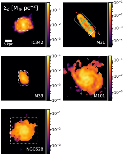
Figure 1: The fitted dust surface densities ($\Sigma_{d}$ [${\rm M_{\odot}\,pc\textsuperscript{-2}}$]) at the common resolution (a Gaussian PSF with FWHM=1.94 kpc). The levels of $\Sigma_{d}$ are indicated by the colorbars attached to each panel. Note that the scales in the panels are not identical. The white dotted line marks the boundary where we have detections in all observations, which we constrain our analysis to. This boundary is defined by CO in most cases. The boundary of M101 is outside the plotting range. The cyan dashed line marks the region removed in M31 due to inclination and lacking metallicity data (see Sect. 2). The scale bar at the top left shows the 5 kpc length for all panels. The dust SED fitting is only performed in regions where $\text{S/N}>1$ in all five Herschel bands. The region with $\text{S/N}\leq 1$ in any of the five Herschel bands appears in black. The $>1\,{\rm dex}$ range in $\Sigma_{d}$ within each galaxy indicates that we resolve the exponential disks at this resolution.

The fitting is done at the common resolution. Figure 1 shows the resulting dust maps. Although the angular resolution has been degraded substantially for some galaxies, the range of $\Sigma_{d}$ at the common resolution is still more than one order of magnitude in each galaxy. This indicates the $\sim 2\,{\rm kpc}$ resolution resolves the exponential disks of our selected galaxies.

2.1.3 Fitting errors

For each model parameter ($X={\rm log}\textsubscript{10}\Sigma_{d}$, $T_{d}$, or $\beta_{2}$), we use the marginalized likelihood-weighted 16-/84-percentile ($X_{16}$ and $X_{84}$, respectively) at each pixel to represent the $1{\text{-}}\sigma$ distribution. We then quote the maximum difference between the expectation value ($X_{\rm exp}$) and the $1{\text{-}}\sigma$ distribution as the fitting error $\epsilon_{X}$, that is:

$$\epsilon_{X}=\max\left((X_{84}-X_{\rm exp}),\ (X_{\rm exp}-X_{16})\right)~{}.$$ (4)

This is the same method as in Chiang et al. (2018).

2.2 Gas masses

We calculate the total gas surface density ($\Sigma_{\rm gas}$) as:

$$\Sigma_{\rm gas}=\Sigma_{\rm atom}+\Sigma_{\rm mol}~{},$$ (5)

where $\Sigma_{\rm atom}$ is the atomic gas surface density and $\Sigma_{\rm mol}$ is the molecular gas surface density.

2.2.1 Atomic gas mass

We use new and archival Hi 21 cm line emission ($I_{\textsc{Hi}}$) data to trace $\Sigma_{\rm atom}$. The data sources are: IC342 (P.I. K. M. Sandstrom; I. Chiang et al. in preparation), M31 (Braun et al., 2009), M33 (Koch et al., 2018), M101 (Walter et al., 2008), and NGC628 (Walter et al., 2008). The resolution of the Hi data is always high enough that it never limits our analysis. For M31 and M33, the two galaxies with largest angular scales, a short-spacing correction with GBT data has been included in the original works (Braun et al., 2009; Koch et al., 2018). The short-spacing correction is not applied in IC342, M101 and NGC628.

Among these three galaxies, IC342 is most likely to have its $I_{\textsc{Hi}}$ underestimated with interferometric data only due to its sky coverage: the Hi 21-cm signal in IC342 spans a diameter $\sim 45\arcmin$, whereas the largest angular scale covered by the VLA D-configuration is $\sim 16\arcmin$ in the L band. The total atomic mass in our IC342 map is $\rm M_{atom}=7.9\times 10^{9}~{}M_{\odot}$, which is close to the $\rm M_{atom}=8.4\times 10^{9}~{}M_{\odot}$ in Crosthwaite et al. (2000, distance corrected). Single-dish measurement in literature (Rots, 1979, distance corrected) showed a $\rm M_{atom}=18.7\times 10^{9}~{}M_{\odot}$. However, this value is expected to be overestimated because the low spatial and velocity resolutions in Rots (1979) data are not enough to distinguish and remove the MW foreground completely.

We also compare our result with the recent single-dish data (EBHIS, Kerp et al., 2011; Winkel et al., 2016). We choose a spectral range that is free from the MW foreground, $\sim 43{-}128$ km/s (the Hi 21-cm signal in IC342 spans $\Delta v\sim 210$ km/s). We find the total flux from EBHIS data is $\sim 1.6$ times larger than our VLA measurement in this range, which indicates that a short-spacing correction is desired but confused by MW foreground emission. Since this 1.6 factor is an average value instead of an offset that can be directly applied to all pixels, we do not include it in our analysis. This factor does not affect our main conclusions due to the low atomic gas content in our region of interest, which is at the center of IC342.

We calculate $\Sigma_{\rm atom}$ from $I_{\textsc{Hi}}$ via the following equation, assuming the opacity is negligible (e.g. Walter et al., 2008):

$$\Sigma_{\rm atom}\,[{\rm M_{\odot}\,pc\textsuperscript{-2}}]=\\ 1.36\times(8.86\times 10^{3})\times\left(\frac{I_{\textsc{Hi}}\,[{\rm Jy\,beam\textsuperscript{-1}\,km\,s\textsuperscript{-1}}]}{{\rm B}\textsubscript{\rm maj}\,[\arcsec]\times{\rm B}\textsubscript{\rm min}\,[\arcsec]}\right)~{},$$ (6)

where B_maj and B_min are the full-width half-maximum (FWHM) of the major and minor axes of the synthesized beam, respectively. The $1.36$ factor accounts for the mass of helium and heavy elements.

2.2.2 Molecular Gas Mass

We use CO rotational line emission ($I_{\rm CO}$) to trace $\Sigma_{\rm mol}$. The data sources are: IC342 (A. Schruba et al. in preparation), M31 (Nieten et al., 2006), M33 (Gratier et al., 2010; Druard et al., 2014), M101 (Leroy et al., 2009), and NGC628 (Leroy et al., 2009). The CO resolution is always high enough that it never limits our analysis.

Throughout the paper, $\alpha_{\rm CO}$ is quoted for the ${{\rm CO}\,J=1\to 0}$ rotational line at 115 GHz and includes a factor to account for helium. However, we use the 230 GHz ${{\rm CO}\,J=2\to 1}$ data in M33, M101, and NGC628. In those cases, we quote a (2-1)$/$(1-0) brightness temperature ratio (R₂₁) to convert the integrated intensity, that is:

$$I_{{\rm CO}\,J=1\to 0}\,[{\rm K\,km\,s\textsuperscript{-1}}]=\frac{I_{{\rm CO}\,J=2\to 1}\,[{\rm K\,km\,s\textsuperscript{-1}}]}{{\rm R}\textsubscript{21}}~{}.$$ (7)

We use ${\rm R}\textsubscript{21}=0.8$ in M33 (Gratier et al., 2010; Druard et al., 2014), and ${\rm R}\textsubscript{21}=0.7$ in M101 and NGC628 (Leroy et al., 2013). We do not include uncertainties resulting from variations of R₂₁ in the analysis. The uncertainty in D/M due to the choice of R₂₁ is $\leq 0.05\,{\rm dex}$ in the three galaxies using CO $\rm J=2\to 1$ data (M33, M101 and NGC628). In M33 and NGC628, the measured variations of R₂₁ are reasonably small (Sandstrom et al., 2013; Druard et al., 2014). While in M101, R₂₁ could increase by $\sim 0.3$ dex in the central $\sim 0.05$ R₂₅ ($\sim 1.2$ kpc, Sandstrom et al., 2013), which indicates that we might underestimate $\Sigma_{\rm mol}$ in that small region. The R₂₁ values adopted in this study are consistent with the PHANGS measurements (${\rm R}\textsubscript{21}=0.64\pm 0.09$, J. den Brok et al. 2020, A&A submitted) considering the systematic uncertainties due to calibration (e.g., 15% for CO $\rm J=2\to 1$ data in Druard et al., 2014).

We can translate $I_{\rm CO}$ to $\Sigma_{\rm mol}$ via a CO-to-H₂ conversion factor ($\alpha_{\rm CO}$):

$$\Sigma_{\rm mol}\,[{\rm M_{\odot}\,pc\textsuperscript{-2}}]=\\ \alpha_{\rm CO}\,[{\rm M_{\odot}\,pc^{-2}\,(K\,km\,s^{-1})^{-1}}]\times I_{{\rm CO}\,J=1\to 0}\,[{\rm K\,km\,s\textsuperscript{-1}}]~{}.$$ (8)

Table 2: List of $\alpha_{\rm CO}$ prescriptions used in this work.

Prescription	$\alpha_{\rm CO}$ formula
	[${\rm M_{\odot}\,pc^{-2}\,(K\,km\,s^{-1})^{-1}}$ ]
$\alpha_{\rm CO}^{\rm MW}$	4.35
$\alpha_{\rm CO}^{\rm S12}$	$8.0\times\rm(Z/Z_{\odot})^{~{}-2.0}$
$\alpha_{\rm CO}^{\rm B13}$	$\rm 2.9\times\exp\left(\frac{0.4}{Z/Z_{\odot}}\right)\times\left\{\begin{array}[]{ll}\left(\Sigma_{\rm Total}^{100}\right)^{-0.5}&,\,\Sigma_{\rm Total}^{100}\geq 1\\ 1&,\,\Sigma_{\rm Total}^{100}<1\end{array}\right.$
$\alpha_{\rm CO}^{\rm H15}$	$\rm 4.35\times\left\{\begin{array}[]{ll}1&,\,Z\geq Z_{\odot}\\ (Z/Z_{\odot})^{-1.96}&,\,Z<Z_{\odot}\end{array}\right.$

Note. — $\Sigma_{\rm Total}^{100}$ is $\Sigma_{\rm Total}$ in $100\,{\rm M_{\odot}\,pc\textsuperscript{-2}}$. $Z/Z_{\odot}=1$ at $12+{\rm log}\textsubscript{10}({\rm O/H})=8.69$ throughout this paper.

Since D/M is sensitive to the choice of $\alpha_{\rm CO}$, we calculate our results with four $\alpha_{\rm CO}$ prescriptions in this study (see Table 2). The conventional MW $\alpha_{\rm CO}$ ($\alpha_{\rm CO}^{\rm MW}$; Solomon et al., 1987; Strong & Mattox, 1996; Abdo et al., 2010) is one of the most widely used choices for $\alpha_{\rm CO}$. It has a fixed value at 4.35 ${\rm M_{\odot}\,pc^{-2}\,(K\,km\,s^{-1})^{-1}}$ and no dependence on the environments (see footnote 1 for the conversion between $\alpha_{\rm CO}$ and $X_{\rm CO}$). The Schruba et al. (2012, their table 7, the “all galaxies” formula with HERACLES sample) prescription ($\alpha_{\rm CO}^{\rm S12}$) models $\alpha_{\rm CO}$ as a simple power law with metallicity, which is a common strategy in modelling $\alpha_{\rm CO}$ (e.g. Israel, 1997; Feldmann et al., 2012; Hunt et al., 2015; Accurso et al., 2017). $\alpha_{\rm CO}^{\rm S12}$ has the largest normalization factor among the prescriptions here, thus it results in the overall highest $\Sigma_{\rm gas}$, or the smallest D/M. Another power-law prescription we include here is the Hunt et al. (2015, Sect. 5.1) prescription ($\alpha_{\rm CO}^{\rm H15}$), which is a power law with metallicity in regions below solar metallicity ($\rm Z_{\odot}$) and a constant at $\alpha_{\rm CO}^{\rm MW}$ above $\rm Z_{\odot}$. This cut off is due to smaller amount of CO-dark H₂ at high metallicity. The Bolatto et al. (2013, Eq. 31) prescription ($\alpha_{\rm CO}^{\rm B13}$) has an exponential dependence on metallicity and a power law dependence on total surface density ($\Sigma_{\rm Total}$ = $\Sigma_{\rm gas}$ + $\Sigma_{\star}$) in the regions with highest surface densities. Note that we assume $\Sigma_{\rm GMC}=100\,{\rm M_{\odot}\,pc\textsuperscript{-2}}$ in the $\alpha_{\rm CO}^{\rm B13}$ case.

2.3 Metallicity

Table 3: 12+log₁₀(O/H) data.

Name	Reference	12+log10(O/H) at the galaxy center	Slope
		[dex]	[${\rm dex}\,{\rm kpc}^{-1}$]	[${\rm dex}\,{\rm R}\textsubscript{25}^{-1}$]
IC342	K. Kreckel et al. in preparation	8.64 ($\pm 0.01$)	-0.012 ($\pm 0.003$)	-0.12 ($\pm 0.03$)
M31	Zurita & Bresolin (2012)	8.72 ($\pm$0.18)	-0.026 ($\pm$0.013)	-0.52 ($\pm$0.26)
M33	Bresolin (2011)	8.50 ($\pm$0.02)	-0.041 ($\pm$0.005)	-0.34 ($\pm$0.04)
M101	Croxall et al. (2016); Berg et al. (2020)	8.78 ($\pm$0.04)	-0.031 ($\pm$0.002)	-0.75 ($\pm$0.06)
NGC628	Berg et al. (2015, 2020)	8.71 ($\pm$0.06)	-0.027 ($\pm$0.007)	-0.38 ($\pm$0.10)

We use the oxygen abundance, 12+log₁₀(O/H), to trace metallicity in this work. We adopt $12+{\rm log}\textsubscript{10}({\rm O/H})_{\odot}=8.69$ (Asplund et al., 2009). We adopt measurements from multiple sources (Table 3). We use gradients of 12+log₁₀(O/H) derived from auroral line measurements in Hii regions in all galaxies except IC342. For IC342, we use the S-calibration for strong lines from Pilyugin & Grebel (2016, hereafter PG16S), which is a calibration showing good agreement with direct metallicity measurements (Croxall et al., 2016; Kreckel et al., 2019). Within the region of interest in this work, the 12+log₁₀(O/H) ranges from 8.2 to 8.8. Note that in M31, the metallicity gradient is derived with data outside 0.4 R₂₅ only (Zurita & Bresolin, 2012), thus we blank all M31 data within 0.4 R₂₅ in the D/M analysis.

In the calculation of D/M, we need to convert the 12+log₁₀(O/H) to metallicity ($Z=\Sigma_{\rm metal}/\Sigma_{\rm gas}$, note that $\Sigma_{\rm gas}$ includes the mass of heavy elements in our notation) because a complete measurement of abundance of all elements is unavailable. We use a fixed oxygen-to-metals ratio, $\rm M_{O}/M_{metal}=0.51$, calculated from the solar neighborhood chemical composition (Lodders, 2003). The complete conversion is:

$$Z=\frac{1}{\rm M_{O}/M_{metal}}\frac{\rm m_{O}}{\rm 1.36m_{H}}10^{\left(12+{\rm log}\textsubscript{10}({\rm O/H})\right)-12}~{},$$ (9)

where $\rm m_{O}$ and $\rm m_{H}$ are the atomic masses for oxygen and hydrogen, respectively; the 1.36 factor converts hydrogen mass to total gas, which is consistent with the conversion in Sect. 2.2. We do not include a correction of [O/H] due to depletion of oxygen in Hii regions, which is estimated to be $\lesssim 0.1\,{\rm dex}$ (Esteban et al., 1998; Peimbert & Peimbert, 2010).

Although we do our best to quote the most reliable metallicity, we would like to remind the readers of two remaining caveats in our methodology: (a) A fixed oxygen-to-metals ratio across all ISM environments might not be true considering the variation of chemical composition in the ISM (e.g. the variation of log₁₀(N/O) in Croxall et al., 2016). Currently, there is no good observational method to characterize this ratio for all environments. Simulation results suggest that it is reasonable to treat it as a constant at this point (e.g. Ma et al., 2016). (b) We use metallicity gradients instead of a complete metallicity map, which might cause an artificial correlation between D/M and galactocentric radius. In massive spiral galaxies, the variation of metallicity is dominated by the radial gradient, and the azimuthal scatter is considered second order. Croxall et al. (2016) and Berg et al. (2015) measure representative azimuthal scatter of $\sim 0.1\,{\rm dex}$ in M101 and NGC628, which is small compared to the radial gradient but non-negligible. Kreckel et al. (2019) found that the typical scatter of 12+log₁₀(O/H) at a given radius in the PHANGS-MUSE samples is small, which is around 0.03 to 0.05 dex. There are ongoing efforts in fitting a complete 12+log₁₀(O/H) map from sightlines of Hii regions (T. Williams et al. in preparation). Their preliminary results also show that the radial gradient dominates the variation in 12+log₁₀(O/H).

2.4 Star Formation Rate and Stellar Mass

We use the GALEX (Martin et al., 2005) and WISE (Wright et al., 2010) maps to trace star formation rate surface density ($\Sigma_{\rm SFR}$) and stellar mass surface density ($\Sigma_{\star}$). For both GALEX and WISE maps, we use the $z$0MGS data products (Leroy et al., 2019) with a resolution of 15″. The correction for the MW extinction in the GALEX maps have been included in the $z$0MGS data products.

The continuum at the GALEX FUV band ($\sim 154\,{\rm nm}$) is dominated by the light from relatively young ($\lesssim 100\,{\rm Myr}$) stars, so we can estimate $\Sigma_{\rm SFR}$ from the FUV flux ($I_{\rm FUV}$). Since interstellar dust absorbs the starlight and re-emits it in the IR (Calzetti et al., 2007; Kennicutt & Evans, 2012), we further improve the estimation by correcting the $I_{\rm FUV}$ with local dust extinction using WISE W4 ($\sim 22\,\mu{\rm m}$) flux ($I_{\rm W4}$). We adopt the hybrid SFR calibrations in table 7 of Leroy et al. (2019):

$$\Sigma_{\rm SFR}\,[{\rm M_{\odot}\,yr}^{-1}\,{\rm kpc}^{-2}]\approx\\ 8.85\times 10^{-2}I_{\rm FUV}\,[{\rm MJy\,sr\textsuperscript{-1}}]+3.02\times 10^{-3}I_{\rm W4}\,[{\rm MJy\,sr\textsuperscript{-1}}]~{}.$$ (10)

Note that although we adopt GALEX FUV maps that have been corrected for the MW extinction, the IC342 $\Sigma_{\rm SFR}$ derived from GALEX FUV could be uncertain due to its high MW extinction. However, the impact is small since the $\Sigma_{\rm SFR}$ is dominated by the WISE W4 term.

We use the WISE W1 ($\sim 3.4\,\mu{\rm m}$) maps to trace $\Sigma_{\star}$. We adopt a stellar-to-W1 mass-to-light ratio, $\Upsilon^{3.4}_{\star}$, from $z$0MGS (Leroy et al., 2019). We then use this $\Upsilon^{3.4}_{\star}$ to calculate $\Sigma_{\star}$ from WISE W1 flux ($I_{\rm W1}$):

$$\Sigma_{\star}\,[{\rm M_{\odot}\,pc\textsuperscript{-2}}]\approx 3.3\times 10^{2}\left(\frac{\Upsilon^{3.4}_{\star}}{0.5}\right)I_{\rm W1}\,[{\rm MJy\,sr\textsuperscript{-1}}]~{}.$$ (11)

2.5 Ratios and Fractions

We use three derived ratios and fractions in the following analysis, which are calculated with the following formulas:

$${\rm D/M}\equiv\frac{\Sigma_{d}}{\Sigma_{\rm metal}}=\frac{\Sigma_{d}}{\Sigma_{\rm gas}\times Z}~{},$$ (12)

$${\rm f}\textsubscript{{\rm H}\textsubscript{2}}\equiv\frac{\Sigma_{\rm mol}}{\Sigma_{\rm gas}}~{},$$ (13)

$${\rm f}\textsubscript{\rm gas}\equiv\frac{\Sigma_{\rm gas}}{\Sigma_{\rm gas}+\Sigma_{\star}}~{}.$$ (14)

Note that whenever we calculate the galaxy-averaged or radial-binned values of these quantities, we calculate the ratio of averages, instead of the average of ratios.

2.6 Dynamical Equilibrium Pressure

We use the mid-plane dynamical equilibrium pressure ($P_{\rm DE}$) to trace the volume density of gas in the ISM. We estimate $P_{\rm DE}$ with the same basic formulism in Elmegreen (1989), Leroy et al. (2008), Gallagher et al. (2018) and Sun et al. (2020):

$$P_{\rm DE}=\frac{\pi G}{2}\Sigma_{\rm gas}^{2}+\Sigma_{\rm gas}\sqrt{2G\rho_{\star}}\sigma_{\rm gas,\,z}~{}.$$ (15)

The first term represents the weight of the ISM due to the self-gravity of the ISM disk ($P_{\rm DE,\,self}$). The second term is the weight of the ISM due to stellar gravity ($P_{\rm DE,\,\star}$). $\sigma_{\rm gas,\,z}$ is the vertical gas velocity dispersion. We adopt a constant value of $\sigma_{\rm gas,\,z}=11\,\rm km\,s^{-1}$ from Leroy et al. (2008). $\rho_{\star}$ is the stellar mass volume density near the mid-plane. We estimate $\rho_{\star}$ with:

$$\rho_{\star}=\frac{\Sigma_{\star}}{4H_{\star}}=\frac{\Sigma_{\star}}{0.12{\rm R}\textsubscript{25}}~{},$$ (16)

where $H_{\star}$ is the stellar scale height. We estimate $H_{\star}$ with a fixed flattening ratio ${\rm R}\textsubscript{25}/H_{\star}=33.6$ (Leroy et al., 2008; Sun et al., 2020). The systematic uncertainty in $P_{\rm DE}$ resulting from the adopted $\sigma_{\rm gas,\,z}$ and the R₂₅-to-$H_{\star}$ conversion is $\sim 0.1{-}0.2$ dex (Leroy et al., 2008; Sun et al., 2020). This is not included in the following Monte Carlo analysis since it is not a random error.

3 D/M and the CO-to-H₂ Conversion Factor

In this section, we propose a novel approach to constraining D/M and $\alpha_{\rm CO}$ simultaneously by examining the resolved environmental dependence of D/M on metallicity and ISM gas density. We expect that if all relevant quantities are accurately measured, we should observe D/M to increase or stay constant with both metallicity and ISM gas density. It has been demonstrated in several depletion-based D/M studies that D/M is positively correlated with both metallicity and gas volume density (Jenkins, 2009, 2014; Roman-Duval et al., 2019b; Péroux & Howk, 2020). From a theoretical perspective, it is also shown that if dust growth dominates over other dust input mechanisms, D/M would be positively correlated with both metallicity and ISM gas density; if the dust growth rate is lower due to either low dust or gas-phase metals abundance, D/M would stay roughly constant (Hirashita, 1999; Inoue, 2003; Zhukovska et al., 2008; Asano et al., 2013; Rowlands et al., 2014; De Vis et al., 2017; Hou et al., 2019; Aoyama et al., 2020).

We take 12+log₁₀(O/H) and $P_{\rm DE}$ as tracers for metallicity and ISM gas density, respectively. We calculate the Pearson correlation coefficients of the radial dependence to quantify the D/M-12+log₁₀(O/H) and D/M-$P_{\rm DE}$ correlations. In Sect. 3.1, we first calculate D/M with four existing $\alpha_{\rm CO}$ prescriptions, and examine the D/M-12+log₁₀(O/H) and D/M-$P_{\rm DE}$ correlations. In Sect. 3.2, we attempt to constrain D/M and $\alpha_{\rm CO}$ simultaneously with the expected correlations. In Sect. 3.3, we summarize the results in the above two sections. We show the profiles of all measurements calculated with $\alpha_{\rm CO}^{\rm B13}$ in Appendix A.

3.1 Inspecting $\alpha_{\rm CO}$ Prescriptions

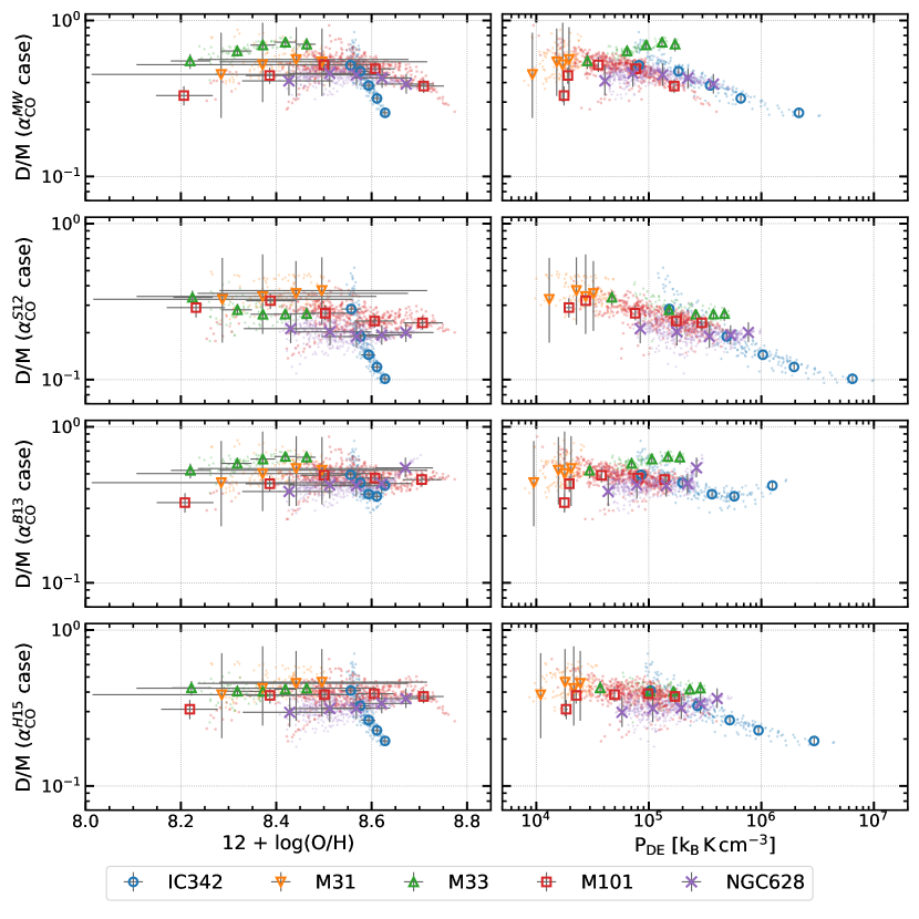
Figure 2: Measured D/M as calculated with four different $\alpha_{\rm CO}$ prescriptions. The large symbols are radial-binned values, while the small, faint symbols are the pixel-by-pixel values where detection is above $3\sigma$. The errorbar shows the 16-/84-percentile distribution from 1000 Monte Carlo tests assuming Gaussian error in measurements. The $x$-axes are 12+log₁₀(O/H) and $P_{\rm DE}$, which are our tracers for metallicity and gas volume density, respectively.

Table 4: Pearson correlation coefficients of the radial D/M-12+log₁₀(O/H) and D/M-$P_{\rm DE}$ dependence within each galaxy. The upper and lower variances are quoted from the 16- and 84-percentiles of 1000 Monte Carlo tests (see text).

Galaxy	Quantity	Prescription
		$\alpha_{\rm CO}^{\rm MW}$	$\alpha_{\rm CO}^{\rm S12}$	$\alpha_{\rm CO}^{\rm B13}$	$\alpha_{\rm CO}^{\rm H15}$
IC342	corr(D/M, 12+log10(O/H))	$-0.99^{+0.02}_{-0.01}$	$-0.99^{+0.01}_{-0.01}$	$-0.65^{+0.23}_{-0.13}$	$-0.99^{+0.01}_{-0.01}$
	corr(D/M, $P_{\rm DE}$)	$-0.89^{+0.01}_{-0.10}$	$-0.78^{+0.01}_{-0.21}$	$-0.31^{+0.01}_{-0.46}$	$-0.83^{+0.01}_{-0.16}$
M31	corr(D/M, 12+log10(O/H))	$0.90^{+0.09}_{-0.99}$	$0.99^{+0.01}_{-1.79}$	$0.92^{+0.07}_{-1.07}$	$0.98^{+0.01}_{-1.25}$
	corr(D/M, $P_{\rm DE}$)	$0.93^{+0.01}_{-0.36}$	$0.54^{+0.21}_{-1.01}$	$0.91^{+0.02}_{-0.38}$	$0.75^{+0.09}_{-0.49}$
M33	corr(D/M, 12+log10(O/H))	$0.94^{+0.02}_{-0.28}$	$-0.89^{+0.35}_{-0.05}$	$0.97^{+0.01}_{-0.43}$	$-0.02^{+0.71}_{-0.60}$
	corr(D/M, $P_{\rm DE}$)	$0.86^{+0.11}_{-0.18}$	$-0.81^{+0.17}_{-0.14}$	$0.91^{+0.05}_{-0.34}$	$0.13^{+0.52}_{-0.78}$
M101	corr(D/M, 12+log10(O/H))	$0.42^{+0.17}_{-0.14}$	$-0.83^{+0.21}_{-0.08}$	$0.82^{+0.07}_{-0.08}$	$0.75^{+0.14}_{-0.20}$
	corr(D/M, $P_{\rm DE}$)	$-0.13^{+0.42}_{-0.01}$	$-0.89^{+0.12}_{-0.08}$	$0.47^{+0.25}_{-0.01}$	$0.40^{+0.34}_{-0.06}$
NGC628	corr(D/M, 12+log10(O/H))	$-0.30^{+0.97}_{-0.43}$	$-0.63^{+1.40}_{-0.27}$	$0.85^{+0.09}_{-0.18}$	$0.96^{+0.03}_{-0.29}$
	corr(D/M, $P_{\rm DE}$)	$-0.62^{+1.22}_{-0.17}$	$-0.46^{+1.18}_{-0.47}$	$0.84^{+0.05}_{-0.26}$	$0.98^{+0.01}_{-0.35}$

We calculate $\Sigma_{\rm gas}$ and D/M with four widely used $\alpha_{\rm CO}$ prescriptions (Sect. 2.2.2), and examine their resulting D/M-environment relations. In Figure 2, we show D/M versus 12+log₁₀(O/H) and $P_{\rm DE}$ calculated from the four $\alpha_{\rm CO}$ prescriptions. The Pearson correlation coefficients of the radial trends within each galaxy are presented in Table 4. The variances of the correlation coefficients are derived with the 16-/84-percentiles from 1000 Monte Carlo tests, assuming Gaussian uncertainties in $\Sigma_{d}$, $\Sigma_{\star}$, $\Sigma_{\rm atom}$, $I_{\rm CO}$, and coefficients in the 12+log₁₀(O/H) gradients.

In Figure 2, we notice that IC342 deviates from the other galaxies in the D/M-12+log₁₀(O/H) trend except for $\alpha_{\rm CO}^{\rm B13}$. We also notice that M31 has large uncertainties in D/M, mainly due to its uncertainties in the metallicity gradient, which makes its correlation coefficients in Table 4 less meaningful.

If we put IC342 and M31 aside for a moment, we find all $\alpha_{\rm CO}$ prescriptions except $\alpha_{\rm CO}^{\rm S12}$ to yield reasonable D/M-12+log₁₀(O/H) and D/M-$P_{\rm DE}$ correlation coefficients. Meanwhile, the correlation coefficients are sensitive to the choice of $\alpha_{\rm CO}$. $\alpha_{\rm CO}^{\rm MW}$ yields significant positive or insignificant D/M-12+log₁₀(O/H) and D/M-$P_{\rm DE}$ correlations. $\alpha_{\rm CO}^{\rm S12}$ yields significant negative correlations in M33 and M101, and insignificant correlations in NGC628. $\alpha_{\rm CO}^{\rm B13}$ yields significant positive correlations. $\alpha_{\rm CO}^{\rm H15}$ yields significant positive correlations in M101 and NGC628, and insignificant correlations in M33.

In IC342, we observe strong negative correlations with small variances with $\alpha_{\rm CO}^{\rm MW}$, $\alpha_{\rm CO}^{\rm S12}$ and $\alpha_{\rm CO}^{\rm H15}$. $\alpha_{\rm CO}^{\rm B13}$ yields weaker and less significant negative correlations. Meanwhile, the D/M-12+log₁₀(O/H) trend in IC342 stays within the range among the other galaxies with $\alpha_{\rm CO}^{\rm B13}$ in Figure 2. One possible reason for the distinct behavior of IC342 is the starburst region in its center, which could affect dust SED fitting and $\alpha_{\rm CO}$ due to its temperature and gas velocity dispersion. Regarding the dust SED fitting in the center, we have a fairly good fit quality ($\chi^{2}\lesssim 1$) and a derived dust temperature ($T_{d}\sim 25\,\rm K$) that can be well described by an MBB within $\lambda=100-500\,\mu{\rm m}$, thus we trust our derived $\Sigma_{d}$. Among the $\alpha_{\rm CO}$ prescriptions, $\alpha_{\rm CO}^{\rm B13}$ is the only one that considers the decrease of $\alpha_{\rm CO}$ due to gas temperature and gas dynamics. These effects are modelled by $\Sigma_{\rm Total}$ in Bolatto et al. (2013). This consideration likely results in the least negative D/M-12+log₁₀(O/H) and D/M-$P_{\rm DE}$ correlation coefficients.

In summary, given that we expect D/M to increase or stay constant with both 12+log₁₀(O/H) and $P_{\rm DE}$, $\alpha_{\rm CO}^{\rm B13}$ seems to give the most reasonable D/M among the four prescriptions across all environments. The D/M calculated with $\alpha_{\rm CO}^{\rm B13}$ has a mean value of 0.46, and a 1-$\sigma$ range spanning $0.40{-}0.58$. $\alpha_{\rm CO}^{\rm MW}$ and $\alpha_{\rm CO}^{\rm H15}$ yield reasonable correlations in M33, M101 and NGC628, but result in strong negative correlations in IC342. Two effects likely contribute to this: (i) the distinct behavior of $\alpha_{\rm CO}$ due to the high $\Sigma_{\rm gas}$ and $\Sigma_{\star}$, which is not considered in $\alpha_{\rm CO}$ prescriptions parameterized by metallicity only, e.g., $\alpha_{\rm CO}^{\rm S12}$ and $\alpha_{\rm CO}^{\rm H15}$; and (ii) due to the high f_H2 in IC342, the variation of $\alpha_{\rm CO}$ has a larger impact on D/M, $P_{\rm DE}$, and their relevant correlations.

3.2 Constraining $\alpha_{\rm CO}$ with D/M-12+log₁₀(O/H) and D/M-$P_{\rm DE}$ Relations

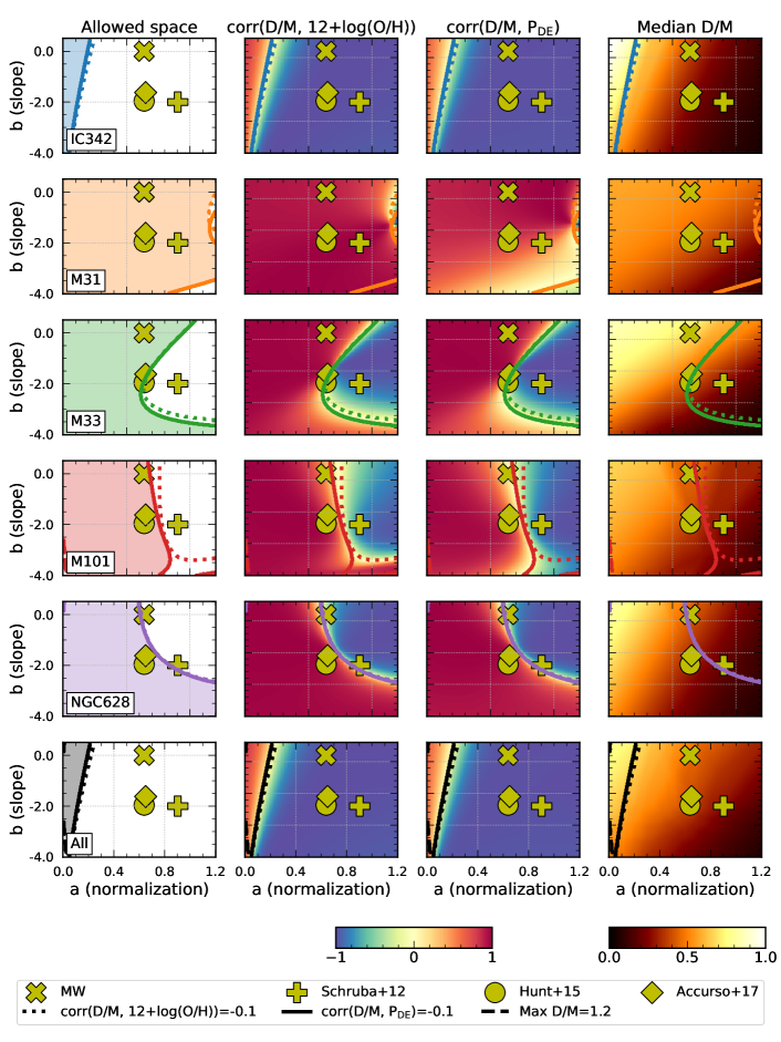
Figure 3: Power-law parameter space with the three constraints in each galaxy. In the “allowed space” column, the shaded area shows the region where all three constraints are satisfied. The x, plus, circle and diamond symbols mark the locations of $\alpha_{\rm CO}^{\rm MW}$, $\alpha_{\rm CO}^{\rm S12}$, $\alpha_{\rm CO}^{\rm H15}$ and the Accurso et al. (2017) $\alpha_{\rm CO}$ in the parameter space, respectively. The dotted, solid and dashed lines show the boundaries of the D/M-12+log₁₀(O/H) correlation, D/M-$P_{\rm DE}$ correlation and the D/M upper limit constraints, respectively. In the central two columns, the colormap shows the Pearson correlation coefficients. In the “Median D/M” column, the colormap shows the pixel-by-pixel median D/M. To fit the 2-dimensional space, we assume $Z<Z_{\odot}$ for $\alpha_{\rm CO}^{\rm H15}$, and assume $\rm\Delta MS=0$ for the Accurso et al. (2017) prescription. All $\alpha_{\rm CO}$ prescriptions shown here locate outside the space satisfying all constraints, which implies that extra parameters are needed in $\alpha_{\rm CO}$ modeling to obtain a reasonable D/M across physical environments.

We demonstrated that the resolved behavior of D/M is sensitive to the assumed conversion factor. Here, we propose a novel approach to constrain $\alpha_{\rm CO}$ by the expected D/M-metallicity and D/M-ISM gas density behaviors, which aims for solving D/M and $\alpha_{\rm CO}$ simultaneously. In the following, we present a first attempt at using this novel method to study the parameter space for the widely-used simple metallicity power-law prescriptions for $\alpha_{\rm CO}$.

We model $\alpha_{\rm CO}$ as a simple power-law parameterized with metallicity, that is,

$${\rm log}\textsubscript{10}\frac{\alpha_{\rm CO}}{1\,{\rm M_{\odot}\,pc^{-2}\,(K\,km\,s^{-1})^{-1}}}=\\ a+b\times\left(12+{\rm log}\textsubscript{10}({\rm O/H})-8.69\right)~{}.$$ (17)

We then constrain the parameter space $[a,\,b]$ to only include the non-negative D/M-12+log₁₀(O/H) and D/M-$P_{\rm DE}$ correlations. We further constrain the parameter space with $\text{D/M}<1$ to ensure the sanity of the resulting prescription. Practically, we relax the lower bound of the correlation coefficient to $\rho>-0.1$ to compensate for uncertainties in measurements. For the same reason, we relax the maximum D/M to $1.2$.

We explore the parameter space $0.0\leq a\leq 1.25$, which is equivalent to a normalization of $0.25\leq\alpha_{\rm CO}/\alpha_{\rm CO}^{\rm MW}\leq 4.0$ at solar metallicity. The range of $b$ is $-4\leq b\leq 0.5$, which generously encompasses the slopes from previous extragalactic studies, which typically find $\alpha_{\rm CO}\propto Z^{-1}$ to $Z^{-3}$ (Bolatto et al., 2013).

The constraints are visualized in the power-law parameter space in Figure 3. In the “allowed space” column, we see the maximum D/M constraints the minimum normalization so that the resulting $\alpha_{\rm CO}$ does not yield unphysical D/M in galaxy centers. The D/M-12+log₁₀(O/H) and D/M-$P_{\rm DE}$ correlations constrain the maximum normalization at fixed slope. They limit the upper bound of $\Sigma_{\rm gas}$, thus the lower bound of D/M, in galaxy centers, so the $\alpha_{\rm CO}$ does not yield negative correlations. The boundary drawn by the two correlation constraints are similar to each other, while the constraint set by the D/M-$P_{\rm DE}$ correlation is usually more strict than the D/M-12+log₁₀(O/H) correlation constraint.

Among the galaxies, IC342 has the narrowest allowed space, which primarily defines the parameter space allowed in all galaxies. The median D/M in this allowed space is high within IC342 and across all galaxies, implying that this space satisfies all constraints by minimizing $\Sigma_{\rm gas}$ and creating a high, flat D/M. In M31, all constraints are easily satisfied within the parameter space we explore. M33, M101, and NGC628 have a large overlapping region in the allowed parameter space. The D/M upper limit constraint in M101 marks part of the boundary of the parameter space allowed in all galaxies.

We overlay four power-law or power-law-like $\alpha_{\rm CO}$ prescriptions, i.e. $\alpha_{\rm CO}^{\rm MW}$, $\alpha_{\rm CO}^{\rm S12}$, $\alpha_{\rm CO}^{\rm H15}$, and the Accurso et al. (2017) prescription, on the parameter space. For $\alpha_{\rm CO}^{\rm H15}$, we only plot its low-metallicity solution. The complete $\alpha_{\rm CO}^{\rm H15}$ formula would be the space between $\alpha_{\rm CO}^{\rm MW}$ and $\alpha_{\rm CO}^{\rm H15}$ in Figure 3. We show Accurso et al. (2017) because it is a widely-used power-law $\alpha_{\rm CO}$. We did not include it in the previous analysis because it yields results similar with $\alpha_{\rm CO}^{\rm S12}$. To fit the Accurso et al. (2017) into the 2-dimensional space, we assume $\rm\Delta MS=0$ in their eq. 25. In M33, M101, and NGC628, these prescriptions sit near the boundary of the correlation constraints. In IC342, these prescriptions are far from the allowed space.

The space that satisfies all constraints in all galaxies (bottom left panel in Figure 3) has a small normalization and a flat slope. The normalization spans $0.2\lesssim\alpha_{\rm CO}/\alpha_{\rm CO}^{\rm MW}\lesssim 0.3$ at solar metallicity, and the slope spans $-1\lesssim b\lesssim 0.5$. Although we do find a parameter space where all constraints are satisfied, it is almost solely defined by IC342. We do not proceed the D/M analysis with this parameter space as it yields a median D/M that seems to high compared to depletion observations.

The results from this test demonstrate that in galaxies except IC342, a simple power law $\alpha_{\rm CO}$ parameterized with metallicity can yield expected physics. Among the tested existing $\alpha_{\rm CO}$ prescriptions, the $\alpha_{\rm CO}^{\rm MW}$, $\alpha_{\rm CO}^{\rm H15}$, and the Accurso et al. (2017) satisfy most constraints in galaxies except IC342, while $\alpha_{\rm CO}^{\rm S12}$ seems to have a normalization that is too high (2$\alpha_{\rm CO}^{\rm MW}$ at $Z_{\odot}$). When we include IC342, the only space that satisfies all constraints yields D/M that seems too high, and the tested existing $\alpha_{\rm CO}$ prescriptions are far outside this allowed space. This suggests that one would probably need a more sophisticated functional form to properly model $\alpha_{\rm CO}$ across all environments (e.g., the starburst region in IC342). One example is the Bolatto et al. (2013) prescription, where the authors attempt to model the decrease of $\alpha_{\rm CO}$ in the high-$\Sigma_{\rm Total}$ regions due to the combined effects of gas temperature and velocity dispersion.

3.3 Section Summary

We showed that the D/M is sensitive to the choice of $\alpha_{\rm CO}$. Among the prescriptions in Sect. 3.1, $\alpha_{\rm CO}^{\rm B13}$ gives the most reasonable D/M. This is inferred from the D/M-12+log₁₀(O/H) and D/M-$P_{\rm DE}$ correlations, especially in IC342. In Sect. 3.2, we use a new approach to constrain D/M and $\alpha_{\rm CO}$ simultaneously. However, in this first attempt, we show that the $\alpha_{\rm CO}$ satisfying all constraints yields D/M too high compared to depletion observations. Thus, we proceed with the $\alpha_{\rm CO}^{\rm B13}$ case for the following analysis.

The median and the 16-/84-percentile of our observed D/M calculated with $\alpha_{\rm CO}^{\rm B13}$ is $0.46^{+0.12}_{-0.06}$. This is consistent with the values adopted in Clark et al. (2016, 2019), which are $0.5\pm 0.1$ and $0.4\pm 0.2$, respectively. The median D/M and the 16-/84-percentile in each galaxy are $0.41^{+0.11}_{-0.05}$, $0.50^{+0.11}_{-0.06}$, $0.60^{+0.05}_{-0.06}$, $0.48^{+0.06}_{-0.05}$ and $0.43^{+0.03}_{-0.04}$ for IC342, M31, M33, M101 and NGC628, respectively. Due to our limited understanding of the CO-to-H₂ conversion factor, we cannot conclusively determine the environmental dependence of D/M. We present the observed environmental dependence calculated with $\alpha_{\rm CO}^{\rm B13}$ in Appendix A.

4 Discussion

4.1 Implications of the Observed D/M

In Sect. 3, we calculate D/M with several common $\alpha_{\rm CO}$ prescriptions and the parameter space of a power-law $\alpha_{\rm CO}$ parameterized by metallicity. Although we have not fully explored all possible descriptions of $\alpha_{\rm CO}$, we proceed the analysis with the most reasonable prescription, $\alpha_{\rm CO}^{\rm B13}$, at the moment. The $\alpha_{\rm CO}^{\rm B13}$ yields a fairly constant D/M over a wide range of physical environments, with a median $\rm D/M=0.46$. From dust evolution simulations (Dwek, 1998; Asano et al., 2013; Aoyama et al., 2020), one possible explanation for a constant D/M is that dust growth dominates the increase of D/M, and the dust growth rate slows down as the available dust-forming metals in gas phase decreases. Thus, D/M would stay roughly constant when most dust-forming metals are already locked in dust grains.

This idea can be demonstrated with the toy model in Aniano et al. (2020), which considers dust growth in the ISM, dust injection from AGB stars and supernovae, and dust destruction. It is assumed that the effective dust growth time scale ($\tau_{a}$) is much smaller than the dust injection time scale ($\tau_{\star}$), thus this model only applies to ISM environments where dust formation is dominated by dust growth in the ISM. With a quasi-steady state assumption, the model gives D/M as a function of metallicity:

$${\rm D/M}=0.5\frac{f_{m}}{Z^{\prime}}\left\{\left(Z^{\prime}-\frac{\tau_{a}}{\tau_{d}}\right)+\left[\left(Z^{\prime}-\frac{\tau_{a}}{\tau_{d}}\right)^{2}+4\frac{\tau_{a}}{\tau_{\star}}Z^{\prime}\right]^{1/2}\right\}~{},$$ (18)

where $\tau_{d}$ is the effective dust destruction time scale; $Z^{\prime}$ is the metallicity relative to solar value. Again, we use $12+{\rm log}\textsubscript{10}({\rm O/H})_{\odot}=8.69$ ; $f_{m}$ is the mass fraction of dust-forming metals to mass of total metals, that is:

$$f_{m}=\frac{\rm Mass~{}of~{}dust{\text{-}}forming~{}metals}{\rm Mass~{}of~{}total~{}metals}~{}.$$ (19)

In Aniano et al. (2020), $f_{m}$ is fixed at $\sim 45.5\%$. The dust injection time scale has minor impact on the prediction. We fix $\tau_{a}/\tau_{\star}=10^{-2}$ through out all models since we expect $\tau_{a}\sim\mathcal{O}(10^{7})$ yr and $\tau_{\star}\sim\mathcal{O}(10^{9})$ yr in the nearby spiral galaxies, e.g., discussions in Draine (2009) and Asano et al. (2013). Note that we do not expect our measurements to follow one single parameter set because the variation in gas density and SFR will reflect on the change in $\tau_{a}/\tau_{d}$ (Asano et al., 2013; Aniano et al., 2020).

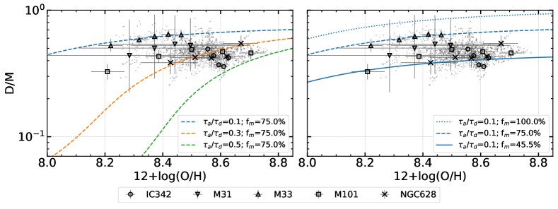
Figure 4: Our measurements and the Aniano et al. (2020) dust evolution model. Left: Fixing $f_{m}$ and varying $\tau_{a}/\tau_{d}$, showing that the variation of D/M is smaller with lower $\tau_{a}/\tau_{d}$. Right: Fixing $\tau_{a}/\tau_{d}$ and varying $f_{m}$, showing that larger $f_{m}$ results in higher D/M. Black: This work. Each marker corresponds to each galaxy as shown in the legend.

We overlay our observed D/M with the model predictions in Figure 4. All the models predict a higher D/M at higher 12+log₁₀(O/H), and the D/M asymptotically approaches $f_{m}$ toward high 12+log₁₀(O/H). In the left panel, we fix $f_{m}=75\%$ and plot three different $\tau_{a}/\tau_{d}$ ratios: 0.1, 0.3 and 0.5. As dust growth becomes faster relative to dust destruction ($\tau_{a}/\tau_{d}$ decreases), the model predicts a smaller variance in D/M in our observed 12+log₁₀(O/H) range. In other words, with a lower $\tau_{a}/\tau_{d}$, D/M approaches $f_{m}$ at a smaller 12+log₁₀(O/H).

In the right panel of Figure 4, we fix $\tau_{a}/\tau_{d}$ at 0.1 and vary $f_{m}$. The major part of our measurements have D/M above the $f_{m}=45.5\%$ model, which means that the fraction of dust-forming metals is probably higher than the value estimated in Aniano et al. (2020). For IC342, M31, M101, and NGC628, most measured D/M values are between the $f_{m}=45.5\%$ and $f_{m}=75\%$ models. This could indicate that the fraction of dust-forming metals is lower than 75% in these galaxies. M33 has the overall highest D/M. Within the frame of this model, it can indicate that the chemical composition of the ISM or dust is different in M33, or $\tau_{a}/\tau_{d}$ in M33 is smaller than in the other galaxies. We will discuss more in Sect. 4.3.

4.2 Previous Multi-Galaxy Observations of D/M

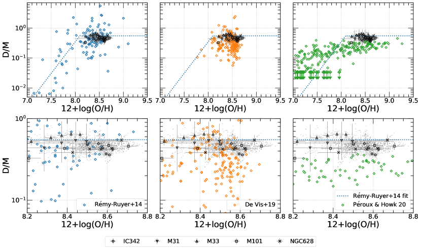
Figure 5: D/M measured in this work overlay with previous observations. Data points with arrows shows the upper limit. Dotted line: the broken power-law fit from Rémy-Ruyer et al. (2014, table 1). Black: This work. Each marker corresponds to each galaxy as shown in the legend. The bottom panels are a zoom-in of the top panels. Left: the Rémy-Ruyer et al. (2014) observations ($\rm X_{CO,\,Z}$ case). Middle: the De Vis et al. (2019) observations (PG16S calibration). Right: the Péroux & Howk (2020) observations. Our measurements are consistent with Rémy-Ruyer et al. (2014) and De Vis et al. (2019), while the Péroux & Howk (2020) measurements are systematically lower than ours.

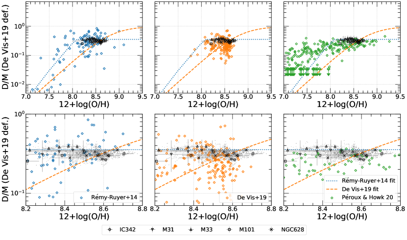
Figure 6: Same as Figure 5, but plotted with the D/M definition in De Vis et al. (2019) (except the Péroux & Howk (2020) data, see main text). Orange dashed line: the De Vis et al. (2019) D/G-12+log₁₀(O/H) fit, converted to D/M-12+log₁₀(O/H) space.

In this section, we compare our measured D/M to previous multi-galaxy D/M observations, including both IR-based and abundance-based measurements. Further, we inspect if there are significant differences in the D/M-metallicity relations between the resolved and galaxy-integrated measurements.

Rémy-Ruyer et al. (2014) and De Vis et al. (2019) are two IR-based galaxy-integrated studies in the nearby universe. With sample size $>100$ galaxies, both works are the benchmarks of our current understanding of the galaxy-integrated dust properties in the nearby universe. Péroux & Howk (2020) derive D/M from elemental abundance ratio with the dust-correction model (De Cia et al., 2016, 2018) in $\gtrsim 200$ Damped Lyman-$\alpha$ systems. Their samples have redshifts ranging $0.1\lesssim z\lesssim 5$, providing us a point of view with different sample selection and methodology. We quote Rémy-Ruyer et al. (2014) data points from their table A.1; De Vis et al. (2019) have their data public on their website; Péroux & Howk (2020) include the data table as one of their supplement materials.

Since De Vis et al. (2019) adopt a different definition of D/M from ours, we show the comparison with both definitions. In this work, we assume that the depletion in Hii regions, where we get the 12+log₁₀(O/H) measurements, is negligible ($\lesssim 0.1\,{\rm dex}$, e.g. Peimbert & Peimbert, 2010); on the other hand, De Vis et al. (2019) assume the 12+log₁₀(O/H) measured in Hii regions only traces gas-phase metals, thus one needs to consider the mass locked in dust grains to get the total metal mass, that is:

$$\rm{(D/M)}_{D19}\equiv\frac{\Sigma_{d}}{\Sigma_{d}+\Sigma_{\rm metal}}~{}.$$ (20)

We show the D/M derived with our definition in Figure 5, and the D/M derived with the De Vis et al. (2019) definition in Figure 6. Note that the Péroux & Howk (2020) measurements are not converted in either figure due to their D/M-derivation methodology. Péroux & Howk (2020) derive D/M with a dust-corrected model (De Cia et al., 2016, 2018), which already includes both the gas-phase metal and metal in dust.

In Figures 5 and 6, we show the Rémy-Ruyer et al. (2014) measurements in the left panels and their fit (the gas-to-dust ratio fit with a broken power-law converted to D/M-to-12+log₁₀(O/H). $\rm X_{CO,\,Z}$ case) in all panels. Our measurements locate roughly in the center of their measurements at the same metallicity, and our measurements are also consistent with their broken power law in the high-metallicity end. Both facts suggest that our D/M-to-metallicity relations are consistent with the Rémy-Ruyer et al. (2014) measurements. Note that in the high-metallicity region, the Rémy-Ruyer et al. (2014) broken power law gives a constant D/M, which matches our measurements that D/M is roughly a constant across galaxies. In Figure 5, there are some Rémy-Ruyer et al. (2014) measurements with $\text{D/M}>1$. Since their adopted $\alpha_{\rm CO}$ (Schruba et al., 2012) has relatively large normalization (see Figure 2), those high D/M values are not likely due to underestimating $\Sigma_{\rm gas}$ from the choice of $\alpha_{\rm CO}$. Instead, it is more likely an issue in the adopted dust opacity function, differences in dust SED fitting techniques, or differences in metallicity calibration.

In the middle panels of Figures 5 and 6, we present the De Vis et al. (2019) measurements (PG16S calibration) and ours. We only select data points where both Hi and H₂ measurements are available in De Vis et al. (2019). We also convert their D/G-12+log₁₀(O/H) fit to a D/M-12+log₁₀(O/H) and plot it in all panels in Figure 6. Note that this fit is not created for the purpose of predicting D/M, thus it is possible to generate unphysical D/M at high metallicity due to its power-law nature in our definition of D/M. Our measured D/M scatters around the upper end of the De Vis et al. (2019) data range in both figures.

We present the Péroux & Howk (2020) measurements in the right panels of Figures 5 and 6. Péroux & Howk (2020) derived their D/M by converting observed elemental abundance ratios into depletion with the empirical formulas in De Cia et al. (2016, 2018). They show that as metallicity increases, D/M increases and the scatter of D/M decreases. This trend is shown over all redshifts. In Figure 5, our measured D/M is systematically higher than the D/M in Péroux & Howk (2020). There are two possible causes for the offset. First, the sample selection in Péroux & Howk (2020) is based on Hi column density and a lot of the data comes from Hi-dominated regions, while most of our data points are in H₂-dominated regions. In other words, the offset might come from the difference in dust evolution in Hi- and H₂-dominated regions. Second, there might be a systematic offset between the IR-based and abundance-based D/M determination.

4.3 The High D/M in M33

In our measurements, we find M33 has a higher D/M than the other galaxies at the same metallicity. One possibility is that the $\alpha_{\rm CO}$ in M33 is larger than $\alpha_{\rm CO}^{\rm B13}$. In Gratier et al. (2010) and Druard et al. (2014), the authors suggest a constant $\alpha_{\rm CO}=2\alpha_{\rm CO}^{\rm MW}$, which is larger than $\alpha_{\rm CO}^{\rm B13}$ everywhere in M33. If we use 2$\alpha_{\rm CO}^{\rm MW}$ for M33, the median D/M in M33 will slightly decrease from 0.60 to 0.56, which brings it closer to the other galaxies.

On the other hand, we could also try to interpret this higher D/M with the Aniano et al. (2020) dust evolution model. The first possibility is that $f_{m}$ is higher in M33. That means the ISM chemical composition is different in M33, and there is a larger fraction of dust-forming metals, or a higher ratio of dust-forming metals to oxygen abundance. The second possibility is a shorter $\tau_{a}$ or a longer $\tau_{d}$ in M33. This explanation is less likely because M33 does not seem to have a higher $P_{\rm DE}$ or $\Sigma_{\rm SFR}$ relative to the other galaxies, which are the two key factors affecting $\tau_{a}$ and $\tau_{d}$.

4.4 Future Perspectives in $\alpha_{\rm CO}$ Constraints

In Sect. 3.1, we show that D/M is sensitive to the choice of $\alpha_{\rm CO}$. We find the most reasonable D/M with $\alpha_{\rm CO}^{\rm B13}$, however, we still have negative D/M-metallicity and D/M-density correlations, especially in IC342. In Sect. 3.2, we demonstrate that a $\alpha_{\rm CO}$ prescription described by simple power law with metallicity is not enough to solve the negative correlations. We need a more complex functional form, or taking the effects from other environmental parameters into account, e.g. gas temperature or velocity dispersion. Unfortunately, we do not have enough data points with high $\Sigma_{\rm Total}$, and currently the fitting results are biased toward the centers of IC342 if we do adopt the Bolatto et al. (2013) functional form with our constraints.

To continue investigating on the effect of $\Sigma_{\rm Total}$, one needs to study nearby galaxies with high resolution $\Sigma_{\rm gas}$ data, e.g., the PHANGS (The Physics at High Angular resolution in Nearby GalaxieS Surveys, A. K. Leroy et al. in preparation) galaxies. Meanwhile, the analysis is also limited by the resolution of dust maps and FIR observations. Among the existing and retired FIR telescopes, Herschel has the highest spatial resolution, $\sim 1.8\,{\rm kpc}$ at a distance of 10 Mpc. The resolution is not enough if we want to resolve a $<1\,{\rm kpc}$ high surface density region. A future mission of FIR photometry at higher resolution is needed to improve our understanding of ISM dust.

Meanwhile, the Bolatto et al. (2013) functional form is less applicable to distant galaxies because it is built on resolved measurements of $\Sigma_{\rm gas}$ and $\Sigma_{\star}$. One possible approach to apply the $\alpha_{\rm CO}^{\rm B13}$ prescription to distant galaxies is to derive a conversion from galaxy-integrated quantities to total molecular gas mass derived with $\alpha_{\rm CO}^{\rm B13}$ in resolved galaxies. A larger sample of galaxies with CO emission, stellar mass, and resolved metallicity measurements is required for this approach. Auxiliary data like SFR and total atomic gas mass might also be helpful in the derivation.

5 Summary

We investigate the relation between dust-to-metals ratio (D/M) and various local ISM environmental quantities in five nearby galaxies: IC342, M31, M33, M101, and NGC628. The multi-wavelength data from both archival and new observations are processed uniformly. A modified blackbody model with a broken power-law emissivity is used to model the dust emission SED, together with the fitting techniques and dust opacity calibration proposed by Gordon et al. (2014) and implemented in Chiang et al. (2018) (Sect. 2.1). We utilize metallicity gradients derived from auroral line measurements in Hii regions to ensure a uniform and high-quality metallicity determination wherever possible. We calibrate and image a new IC342 Hi 21 cm map from new VLA observations. This is part of the observations in the EveryTHINGS project (P.I. K. M. Sandstrom; I. Chiang et al. in preparation). All maps are convolved to a common physical resolution at $\sim 2\,{\rm kpc}$ for a uniform analysis.

We propose a new approach to constrain D/M and the CO-to-H₂ conversion factors ($\alpha_{\rm CO}$), that is, we use the expected D/M-metallicity and D/M-ISM gas density correlations measured by depletion studies to evaluate the results. We use this conceptual approach to examine the D/M yielded by existing $\alpha_{\rm CO}$ prescriptions, and demonstrate our first attempt in utilizing this approach to constrain simple metallicity power-law $\alpha_{\rm CO}$. We find the following key points:

1. Among the prescriptions we test, $\alpha_{\rm CO}^{\rm B13}$ yields the most reasonable D/M.

2. With $\alpha_{\rm CO}^{\rm B13}$, the D/M is roughly a constant ($0.46^{+0.12}_{-0.06}$) across a large range of ISM environments.

3. When we exclude IC342, $\alpha_{\rm CO}^{\rm MW}$ and $\alpha_{\rm CO}^{\rm H15}$ can satisfy most constraints set by the D/M-metallicity and D/M-$P_{\rm DE}$ correlations, while $\alpha_{\rm CO}^{\rm S12}$ seems to have a normalization that is too high (2$\alpha_{\rm CO}^{\rm MW}$ at $Z_{\odot}$).

4. The most obvious difference between $\alpha_{\rm CO}^{\rm B13}$ and other prescriptions is the dependence on the total surface density ($\Sigma_{\rm Total}=\Sigma_{\rm gas}+\Sigma_{\star}$), which decreases $\alpha_{\rm CO}$ in the regions with $\Sigma_{\rm Total}>100\,{\rm M_{\odot}\,pc\textsuperscript{-2}}$. This is mostly important in the centers of galaxies, and likely starburst regions.

5. To properly account for the H₂ gas in IC342, it seems that an $\alpha_{\rm CO}$ prescription parameterized by 12+log₁₀(O/H) only is not enough. The $\alpha_{\rm CO}^{\rm B13}$, which depends on $\Sigma_{\rm Total}$, yields the most reasonable D/M in IC342.

6. New FIR observations with spatial resolution better than Herschel are needed for investigating D/M and $\alpha_{\rm CO}$ at high surface density regions.

In Sect. 4, we interpret our observations with the dust evolution model from Aniano et al. (2020). We also compare our results to the previous galaxy-integrated D/M measurements. We find the following implications regarding our results:

1. The roughly constant D/M implies a shorter dust growth time scale ($\tau_{a}$) relative to the dust destruction time scale ($\tau_{d}$).

2. Most of our measurements fall in the range between $f_{m}=45.5\%$ and $f_{m}=75\%$, with $f_{m}$ being the mass fraction of dust forming metals.

3. Our measured D/M is consistent with previous IR-based, galaxy-integrated measurements in the nearby universe (Rémy-Ruyer et al., 2014; De Vis et al., 2019).

4. However, our results are systematically higher than the D/M measured in the abundance-based measurements by Péroux & Howk (2020). This could indicate a systematic offset between IR-based and abundance-based methods.

Our results demonstrate that D/M is sensitive to the choice of $\alpha_{\rm CO}$. The $\alpha_{\rm CO}^{\rm B13}$ is our current best choice of $\alpha_{\rm CO}$, which models the decrease of $\alpha_{\rm CO}$ due to gas temperature and velocity dispersion. Our results show a roughly constant D/M across ISM environments. Further investigation is needed to constrain D/M and $\alpha_{\rm CO}$ simultaneously.

Appendix A Measurements with $\alpha_{\rm CO}^{\rm B13}$

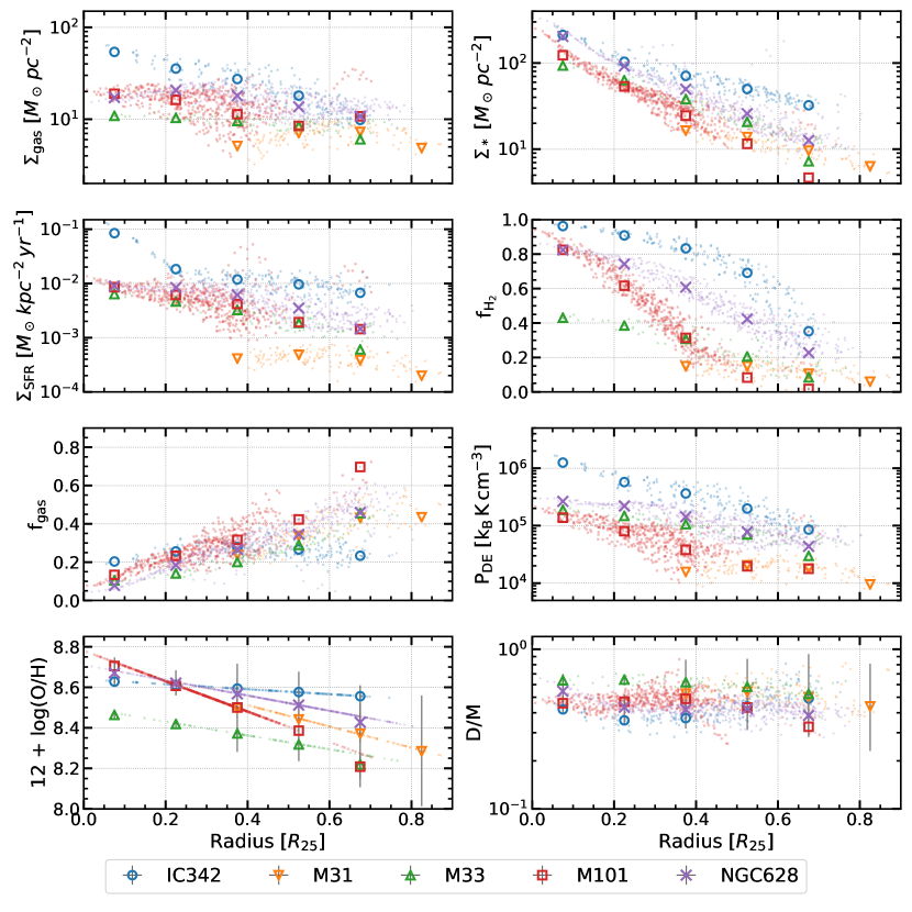
Figure 7: Radial profiles of the observed and derived quantities calculated with $\alpha_{\rm CO}^{\rm B13}$. Small markers: pixel-by-pixel data where detection is above $3\sigma$. Large markers: average in radial bins. The errorbar shows the 16-/84-percentile distribution from 1000 Monte Carlo tests, assuming Gaussian error in measurements.

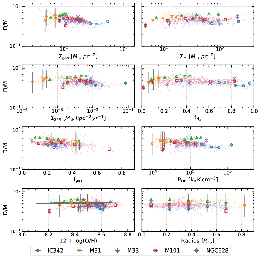
Figure 8: Relations between the physical quantities and D/M calculated with $\alpha_{\rm CO}^{\rm B13}$. The variation of D/M is minimum across all quantities displayed. Small markers: pixel-by-pixel data where detection is above $3\sigma$. Large markers: average in radial bins. The errorbar shows the 16-/84-percentile distribution from 1000 Monte Carlo tests, assuming Gaussian error in measurements.

As we have stated in Sect. 3.3, due to our limited understanding of the CO-to-H₂ conversion factor, we do not intend to conclusively determine the environmental dependence of D/M with the current measurements. However, it is still informative to show our measurements with $\alpha_{\rm CO}^{\rm B13}$ here. We present the radial profiles of the measured and derived quantities in Figure 7. D/M is roughly constant as radius increases. On the other hand, most measured quantities decreases as radius increases except f_gas, which increases with radius.

Figure 8 shows the relationship between the physical quantities and D/M. Generally speaking, the D/M is roughly constant across most physical environments. We also notice D/M tend to decrease as f_gas increases, which is a similar trend found in the galaxy-integrated measurements in De Vis et al. (2019).

References

- Abdo et al. (2010) Abdo, A. A., Ackermann, M., Ajello, M., et al. 2010, ApJ, 710, 133
- Accurso et al. (2017) Accurso, G., Saintonge, A., Catinella, B., et al. 2017, MNRAS, 470, 4750
- Aniano et al. (2011) Aniano, G., Draine, B. T., Gordon, K. D., & Sandstrom, K. 2011, PASP, 123, 1218
- Aniano et al. (2020) Aniano, G., Draine, B. T., Hunt, L. K., et al. 2020, ApJ, 889, 150
- Aoyama et al. (2020) Aoyama, S., Hirashita, H., & Nagamine, K. 2020, MNRAS, 491, 3844
- Asano et al. (2013) Asano, R. S., Takeuchi, T. T., Hirashita, H., & Inoue, A. K. 2013, Earth, Planets, and Space, 65, 213
- Asplund et al. (2009) Asplund, M., Grevesse, N., Sauval, A. J., & Scott, P. 2009, ARA&A, 47, 481
- Astropy Collaboration et al. (2013) Astropy Collaboration, Robitaille, T. P., Tollerud, E. J., et al. 2013, A&A, 558, A33
- Astropy Collaboration et al. (2018) Astropy Collaboration, Price-Whelan, A. M., Sipőcz, B. M., et al. 2018, AJ, 156, 123
- Berg et al. (2020) Berg, D. A., Pogge, R. W., Skillman, E. D., et al. 2020, ApJ, 893, 96
- Berg et al. (2015) Berg, D. A., Skillman, E. D., Croxall, K. V., et al. 2015, ApJ, 806, 16
- Bernstein et al. (2002) Bernstein, R. A., Freedman, W. L., & Madore, B. F. 2002, ApJ, 571, 56
- Bolatto et al. (2013) Bolatto, A. D., Wolfire, M., & Leroy, A. K. 2013, ARA&A, 51, 207
- Boquien et al. (2011) Boquien, M., Calzetti, D., Combes, F., et al. 2011, AJ, 142, 111
- Braun et al. (2009) Braun, R., Thilker, D. A., Walterbos, R. A. M., & Corbelli, E. 2009, ApJ, 695, 937
- Bresolin (2011) Bresolin, F. 2011, ApJ, 730, 129
- Buat et al. (2012) Buat, V., Noll, S., Burgarella, D., et al. 2012, A&A, 545, A141
- Calzetti (2001) Calzetti, D. 2001, PASP, 113, 1449
- Calzetti et al. (2007) Calzetti, D., Kennicutt, R. C., Engelbracht, C. W., et al. 2007, ApJ, 666, 870
- Cazaux & Tielens (2004) Cazaux, S., & Tielens, A. G. G. M. 2004, ApJ, 604, 222
- Chiang et al. (2018) Chiang, I.-D., Sandstrom, K. M., Chastenet, J., et al. 2018, ApJ, 865, 117
- Clark et al. (2016) Clark, C. J. R., Schofield, S. P., Gomez, H. L., & Davies, J. I. 2016, MNRAS, 459, 1646
- Clark et al. (2019) Clark, C. J. R., De Vis, P., Baes, M., et al. 2019, MNRAS, 489, 5256
- Compiègne et al. (2011) Compiègne, M., Verstraete, L., Jones, A., et al. 2011, A&A, 525, A103
- Corbelli et al. (2010) Corbelli, E., Lorenzoni, S., Walterbos, R., Braun, R., & Thilker, D. 2010, A&A, 511, A89
- Cormier et al. (2018) Cormier, D., Bigiel, F., Jiménez-Donaire, M. J., et al. 2018, MNRAS, 475, 3909
- Crosthwaite et al. (2000) Crosthwaite, L. P., Turner, J. L., & Ho, P. T. P. 2000, AJ, 119, 1720
- Croxall et al. (2016) Croxall, K. V., Pogge, R. W., Berg, D. A., Skillman, E. D., & Moustakas, J. 2016, ApJ, 830, 4
- Dalcanton et al. (2015) Dalcanton, J. J., Fouesneau, M., Hogg, D. W., et al. 2015, ApJ, 814, 3
- De Cia et al. (2016) De Cia, A., Ledoux, C., Mattsson, L., et al. 2016, A&A, 596, A97
- De Cia et al. (2018) De Cia, A., Ledoux, C., Petitjean, P., & Savaglio, S. 2018, A&A, 611, A76
- De Vis et al. (2017) De Vis, P., Gomez, H. L., Schofield, S. P., et al. 2017, MNRAS, 471, 1743
- De Vis et al. (2019) De Vis, P., Jones, A., Viaene, S., et al. 2019, A&A, 623, A5
- Draine (2003) Draine, B. T. 2003, ApJ, 598, 1017
- Draine (2009) Draine, B. T. 2009, in Astronomical Society of the Pacific Conference Series, Vol. 414, Cosmic Dust - Near and Far, ed. T. Henning, E. Grün, & J. Steinacker, 453
- Draine & Li (2007) Draine, B. T., & Li, A. 2007, ApJ, 657, 810
- Draine et al. (2014) Draine, B. T., Aniano, G., Krause, O., et al. 2014, ApJ, 780, 172
- Druard et al. (2014) Druard, C., Braine, J., Schuster, K. F., et al. 2014, A&A, 567, A118
- Dwek (1998) Dwek, E. 1998, ApJ, 501, 643
- Elmegreen (1989) Elmegreen, B. G. 1989, ApJ, 338, 178
- Esteban et al. (1998) Esteban, C., Peimbert, M., Torres-Peimbert, S., & Escalante, V. 1998, MNRAS, 295, 401
- Fanciullo et al. (2015) Fanciullo, L., Guillet, V., Aniano, G., et al. 2015, A&A, 580, A136
- Feldmann et al. (2012) Feldmann, R., Gnedin, N. Y., & Kravtsov, A. V. 2012, ApJ, 747, 124
- Fritz et al. (2012) Fritz, J., Gentile, G., Smith, M. W. L., et al. 2012, A&A, 546, A34
- Gallagher et al. (2018) Gallagher, M. J., Leroy, A. K., Bigiel, F., et al. 2018, ApJ, 858, 90
- Galliano et al. (2018) Galliano, F., Galametz, M., & Jones, A. P. 2018, ARA&A, 56, 673
- Glover & Clark (2012) Glover, S. C. O., & Clark, P. C. 2012, MNRAS, 421, 9
- Glover & Mac Low (2011) Glover, S. C. O., & Mac Low, M. M. 2011, MNRAS, 412, 337
- Gordon et al. (2014) Gordon, K. D., Roman-Duval, J., Bot, C., et al. 2014, ApJ, 797, 85
- Gould & Salpeter (1963) Gould, R. J., & Salpeter, E. E. 1963, ApJ, 138, 393
- Gratier et al. (2010) Gratier, P., Braine, J., Rodriguez-Fernandez, N. J., et al. 2010, A&A, 522, A3
- Griffin et al. (2010) Griffin, M. J., Abergel, A., Abreu, A., et al. 2010, A&A, 518, L3
- Groves et al. (2012) Groves, B., Krause, O., Sandstrom, K., et al. 2012, MNRAS, 426, 892
- Hildebrand (1983) Hildebrand, R. H. 1983, QJRAS, 24, 267
- Hirashita (1999) Hirashita, H. 1999, ApJ, 510, L99
- Hirashita & Aoyama (2019) Hirashita, H., & Aoyama, S. 2019, MNRAS, 482, 2555
- Hirashita & Kuo (2011) Hirashita, H., & Kuo, T.-M. 2011, MNRAS, 416, 1340
- Hou et al. (2019) Hou, K.-C., Aoyama, S., Hirashita, H., Nagamine, K., & Shimizu, I. 2019, MNRAS, 485, 1727
- Hu et al. (2019) Hu, C.-Y., Zhukovska, S., Somerville, R. S., & Naab, T. 2019, MNRAS, 487, 3252
- Hunt et al. (2015) Hunt, L. K., García-Burillo, S., Casasola, V., et al. 2015, A&A, 583, A114
- Hunter (2007) Hunter, J. D. 2007, CSE, 9, 90
- Inoue (2003) Inoue, A. K. 2003, PASJ, 55, 901
- Israel (1997) Israel, F. P. 1997, A&A, 328, 471
- Israel (2020) —. 2020, A&A, 635, A131
- Issa et al. (1990) Issa, M. R., MacLaren, I., & Wolfendale, A. W. 1990, A&A, 236, 237
- Jenkins (1989) Jenkins, E. 1989, in IAU Symposium, Vol. 135, Interstellar Dust, ed. L. J. Allamandola & A. G. G. M. Tielens, 23
- Jenkins (1987) Jenkins, E. B. 1987, Element Abundances in the Interstellar Atomic Material, Vol. 134 (D. Reidel Publishing Company), 533
- Jenkins (2009) —. 2009, ApJ, 700, 1299
- Jenkins (2014) —. 2014, arXiv e-prints, arXiv:1402.4765
- Jenkins & Wallerstein (2017) Jenkins, E. B., & Wallerstein, G. 2017, ApJ, 838, 85
- Jones et al. (2017) Jones, A. P., Köhler, M., Ysard, N., Bocchio, M., & Verstraete, L. 2017, A&A, 602, A46
- Joye & Mandel (2003) Joye, W. A., & Mandel, E. 2003, in Astronomical Society of the Pacific Conference Series, Vol. 295, Astronomical Data Analysis Software and Systems XII, ed. H. E. Payne, R. I. Jedrzejewski, & R. N. Hook, 489
- Kennicutt & Evans (2012) Kennicutt, R. C., & Evans, N. J. 2012, ARA&A, 50, 531
- Kennicutt et al. (2011) Kennicutt, R. C., Calzetti, D., Aniano, G., et al. 2011, PASP, 123, 1347
- Kerp et al. (2011) Kerp, J., Winkel, B., Ben Bekhti, N., Flöer, L., & Kalberla, P. M. W. 2011, Astronomische Nachrichten, 332, 637
- Kewley & Ellison (2008) Kewley, L. J., & Ellison, S. L. 2008, ApJ, 681, 1183
- Koch et al. (2018) Koch, E. W., Rosolowsky, E. W., Lockman, F. J., et al. 2018, MNRAS, 479, 2505
- Kramer et al. (2010) Kramer, C., Buchbender, C., Xilouris, E. M., et al. 2010, A&A, 518, L67
- Kreckel et al. (2019) Kreckel, K., Ho, I. T., Blanc, G. A., et al. 2019, ApJ, 887, 80
- Krumholz et al. (2011) Krumholz, M. R., Leroy, A. K., & McKee, C. F. 2011, ApJ, 731, 25
- Lang et al. (2020) Lang, P., Meidt, S. E., Rosolowsky, E., et al. 2020, ApJ, 897, 122
- Leroy et al. (2008) Leroy, A. K., Walter, F., Brinks, E., et al. 2008, AJ, 136, 2782
- Leroy et al. (2009) Leroy, A. K., Walter, F., Bigiel, F., et al. 2009, AJ, 137, 4670
- Leroy et al. (2011) Leroy, A. K., Bolatto, A., Gordon, K., et al. 2011, ApJ, 737, 12
- Leroy et al. (2013) Leroy, A. K., Walter, F., Sandstrom, K., et al. 2013, AJ, 146, 19
- Leroy et al. (2019) Leroy, A. K., Sandstrom, K. M., Lang, D., et al. 2019, ApJS, 244, 24
- Li et al. (2019) Li, Q., Narayanan, D., & Davé, R. 2019, MNRAS, 490, 1425
- Lisenfeld & Ferrara (1998) Lisenfeld, U., & Ferrara, A. 1998, ApJ, 496, 145
- Lodders (2003) Lodders, K. 2003, ApJ, 591, 1220
- Ma et al. (2016) Ma, X., Hopkins, P. F., Faucher-Giguère, C.-A., et al. 2016, MNRAS, 456, 2140
- Makarov et al. (2014) Makarov, D., Prugniel, P., Terekhova, N., Courtois, H., & Vauglin, I. 2014, A&A, 570, A13
- Martin et al. (2005) Martin, D. C., Fanson, J., Schiminovich, D., et al. 2005, ApJ, 619, L1
- McKinney (2010) McKinney, W. 2010, in Proceedings of the 9th Python in Science Conference, ed. S. van der Walt & J. Millman, 51
- McMullin et al. (2007) McMullin, J. P., Waters, B., Schiebel, D., Young, W., & Golap, K. 2007, in Astronomical Society of the Pacific Conference Series, Vol. 376, Astronomical Data Analysis Software and Systems XVI, ed. R. A. Shaw, F. Hill, & D. J. Bell, 127
- McQuinn et al. (2017) McQuinn, K. B. W., Skillman, E. D., Dolphin, A. E., Berg, D., & Kennicutt, R. 2017, AJ, 154, 51
- Nieten et al. (2006) Nieten, C., Neininger, N., Guélin, M., et al. 2006, A&A, 453, 459
- Peimbert & Peimbert (2010) Peimbert, A., & Peimbert, M. 2010, ApJ, 724, 791
- Péroux & Howk (2020) Péroux, C., & Howk, J. C. 2020, ARA&A, 58, annurev
- Pilbratt et al. (2010) Pilbratt, G. L., Riedinger, J. R., Passvogel, T., et al. 2010, A&A, 518, L1
- Pilyugin & Grebel (2016) Pilyugin, L. S., & Grebel, E. K. 2016, MNRAS, 457, 3678
- Planck Collaboration et al. (2016) Planck Collaboration, Ade, P. A. R., Aghanim, N., et al. 2016, A&A, 586, A132
- Poglitsch et al. (2010) Poglitsch, A., Waelkens, C., Geis, N., et al. 2010, A&A, 518, L2
- Reach et al. (1995) Reach, W. T., Dwek, E., Fixsen, D. J., et al. 1995, ApJ, 451, 188
- Relaño et al. (2020) Relaño, M., Lisenfeld, U., Hou, K. C., et al. 2020, A&A, 636, A18
- Rémy-Ruyer et al. (2014) Rémy-Ruyer, A., Madden, S. C., Galliano, F., et al. 2014, A&A, 563, A31
- Roman-Duval et al. (2017) Roman-Duval, J., Bot, C., Chastenet, J., & Gordon, K. 2017, ApJ, 841, 72
- Roman-Duval et al. (2014) Roman-Duval, J., Gordon, K. D., Meixner, M., et al. 2014, ApJ, 797, 86
- Roman-Duval et al. (2019a) Roman-Duval, J., Aloisi, A., Gordon, K., et al. 2019a, BAAS, 51, 458
- Roman-Duval et al. (2019b) Roman-Duval, J., Jenkins, E. B., Williams, B., et al. 2019b, ApJ, 871, 151
- Rots (1979) Rots, A. H. 1979, A&A, 80, 255
- Rowlands et al. (2014) Rowlands, K., Gomez, H. L., Dunne, L., et al. 2014, MNRAS, 441, 1040
- Sandstrom et al. (2013) Sandstrom, K. M., Leroy, A. K., Walter, F., et al. 2013, ApJ, 777, 5
- Schruba et al. (2012) Schruba, A., Leroy, A. K., Walter, F., et al. 2012, AJ, 143, 138
- Schruba et al. (2017) Schruba, A., Leroy, A. K., Kruijssen, J. M. D., et al. 2017, ApJ, 835, 278
- Schwartz (1982) Schwartz, P. R. 1982, ApJ, 252, 589
- Sofue et al. (1999) Sofue, Y., Tutui, Y., Honma, M., et al. 1999, ApJ, 523, 136
- Solomon et al. (1987) Solomon, P. M., Rivolo, A. R., Barrett, J., & Yahil, A. 1987, ApJ, 319, 730
- Strong & Mattox (1996) Strong, A. W., & Mattox, J. R. 1996, A&A, 308, L21
- Sun et al. (2020) Sun, J., Leroy, A. K., Ostriker, E. C., et al. 2020, ApJ, 892, 148
- Tully et al. (2009) Tully, R. B., Rizzi, L., Shaya, E. J., et al. 2009, AJ, 138, 323
- van der Walt et al. (2011) van der Walt, S., Colbert, S. C., & Varoquaux, G. 2011, CSE, 13, 22
- Vílchez et al. (2019) Vílchez, J. M., Relaño, M., Kennicutt, R., et al. 2019, MNRAS, 483, 4968
- Walter et al. (2008) Walter, F., Brinks, E., de Blok, W. J. G., et al. 2008, AJ, 136, 2563
- Winkel et al. (2016) Winkel, B., Kerp, J., Flöer, L., et al. 2016, A&A, 585, A41
- Wolfire et al. (2010) Wolfire, M. G., Hollenbach, D., & McKee, C. F. 2010, ApJ, 716, 1191
- Wright et al. (2010) Wright, E. L., Eisenhardt, P. R. M., Mainzer, A. K., et al. 2010, AJ, 140, 1868
- Wu et al. (2014) Wu, P.-F., Tully, R. B., Rizzi, L., et al. 2014, AJ, 148, 7
- Xilouris et al. (2012) Xilouris, E. M., Tabatabaei, F. S., Boquien, M., et al. 2012, A&A, 543, A74
- Yamasawa et al. (2011) Yamasawa, D., Habe, A., Kozasa, T., et al. 2011, ApJ, 735, 44
- Zhukovska (2014) Zhukovska, S. 2014, A&A, 562, A76
- Zhukovska et al. (2016) Zhukovska, S., Dobbs, C., Jenkins, E. B., & Klessen, R. S. 2016, ApJ, 831, 147
- Zhukovska et al. (2008) Zhukovska, S., Gail, H.-P., & Trieloff, M. 2008, A&A, 479, 453
- Zurita & Bresolin (2012) Zurita, A., & Bresolin, F. 2012, MNRAS, 427, 1463