Two-Step Meta-Learning for Time-Series Forecasting Ensemble 

Abstract

Amounts of historical data collected increase and business intelligence applicability with automatic forecasting of time series are in high demand. While no single time series modeling method is universal to all types of dynamics, forecasting using an ensemble of several methods is often seen as a compromise. Instead of fixing ensemble diversity and size, we propose to predict these aspects adaptively using meta-learning. Meta-learning here considers two separate random forest regression models, built on 390 time-series features, to rank 22 univariate forecasting methods and recommend ensemble size. The forecasting ensemble is consequently formed from methods ranked as the best, and forecasts are pooled using either simple or weighted average (with a weight corresponding to reciprocal rank). The proposed approach was tested on 12561 micro-economic time-series (expanded to 38633 for various forecasting horizons) of M4 competition where meta-learning outperformed Theta and Comb benchmarks by relative forecasting errors for all data types and horizons. Best overall results were achieved by weighted pooling with a symmetric mean absolute percentage error of 9.21% versus 11.05% obtained using the Theta method.

Keywords: business intelligence, univariate time-series model, forecasting ensemble, meta-learning, random forest, M4 competition

1 Introduction

Forecasting key performance indicators and any essential dynamics for an organization should be a high-priority business intelligence task. The aim is to envisage indicator values into the future, based on historical observations. An accurate forecast mitigates uncertainties about the future outlook and can reduce errors in decisions and planning, directly influencing the achievability of goals and contributing to risk management. Forecasting should be an integral part of the decision-making activities in management [Hyndman, 2010] since the strategic success of the organization depends upon the practical relation between accuracy of forecast and flexibility of resource allocation plan [Wacker and Lummus, 2002]. It is expected that increasing amounts of historical data records, which constitute valuable resources for the forecasting task, will facilitate accurate forecasting and boost these forecasts’ importance. Although [Petropoulos et al., 2014], while researching main determinants of forecasting accuracy, found that increasing time-series length has a small positive effect on forecasting accuracy, which contradicts insights from the machine learning and deep learning fields.

Almost 40 years ago worldwide, Makridakis forecasting competitions had started (organized in 1982, 1993, 2000, 2018, and 2020) with a goal to benchmark progress in forecasting techniques and derive scientific insights in time-series forecasting. During these events, teams of participants compete to obtain forecasts for ever-increasing amounts of time-series from diverse fields. Results are summarized into recommendations on the usefulness of various time-series models or their ensembles. In the recent M4 competition [Makridakis et al., 2018] the leading forecasting techniques (12 from 17 most accurate ones) featured model ensembles that pool forecasts of several, mainly statistical, models. The best solution was submitted by Uber Technologies, where the hybrid technique combined a statistical forecasting model with neural network architecture. The next most successful submission [Montero-Manso et al., 2020] featured an ensemble of statistical models where weights were thoroughly tuned, and the machine learning model learned these weight recommendations for later prediction. Insights after an older M3 competition [Makridakis and Hibon, 2000] were that forecasts from univariate time-series models almost always (except for annual data) are more accurate than forecasts from multivariate time-series models with external variables (i.e., macroeconomic indicators). Comparison between univariate approaches revealed that more complex models do not guarantee higher accuracy.

Proceeding from results of Makridakis competitions [Makridakis et al., 2018, Makridakis and Hibon, 2000] and numerous academic researches [Clemen, 1989, Hansen and Salamon, 1990, Hendry and Clements, 2004, Timmermann, 2006, Kolassa, 2011] it can be concluded that an ensemble of univariate time-series models often outperforms the best member of the ensemble with respect to forecasting accuracy. The success of forecasting ensemble lies in the diversity of its members [Oliveira and Torgo, 2015], which contributes to robustness against concept drift [Zang et al., 2014] and enhances algorithmic stability [Zou and Yang, 2004]. Besides ensemble diversity, the individual accuracy of its members is also of utmost importance [Lemke and Gabrys, 2010]. A simple arithmetic average with all members weighted equally often outperforms more complex strategies for combining forecasts from several models. Advanced strategies seek to find optimal weights, for example, based on the model’s Akaike information criterion [Kolassa, 2011] or model’s in-sample forecasting errors [Smith and Wallis, 2009] on the last dynamics of time-series in question. In practice, to avoid corrupting the final forecast by a single inaccurate model, variants of robust average or simply median are recommended in forecast pooling [Hendry and Clements, 2004]. Choice of weights for ensemble members often relies upon in-sample forecasting errors. However, when the approximate ranking of the model pool is available instead of exact errors, the weight could be derived from the model’s reciprocal rank [Aiolfi and Timmermann, 2006].

There exists no forecasting method that performs best on all types of time-series [Bauer et al., 2020]. However, efforts to create more universal approaches seek to adjust ensemble size and choose potential members or weights adaptively based on dynamics we try to extrapolate into the future. The argument that the relative accuracy of forecasting methods depends upon the properties of the time-series and information on dynamics at hand can be exploited to choose a suitable model is an old one [Reid, 1972].

Our research explores an adaptive construction of a forecasting ensemble consisting of various statistical and a few machine learning methods with a meta-learning approach. Meta-learners here seek to rank a pool of methods and recommend ensemble size based on historical time-series data characteristics. Recommendations of introduced forecasting assistants are based on training regression meta-models through forecasting experiments on a diverse set of real-world examples - micro-economic time-series from M4 competition. Experiments compare introduced forecasting ensemble based on recommendations from assistants with the best benchmark methods from M4 competition - Theta and Comb, which were outperformed only by 17 out of 49 submissions in M4 competition [Makridakis et al., 2018, Makridakis et al., 2020].

2 Related work

The usefulness of statistics summarizing the data available in a time-series in predicting the relative accuracy of different forecasting methods was explored in [Meade, 2000] where they created regression models to predict the expected error of the forecasting method for the time-series at hand. More similar research to our idea of forecasting assistants, after early expert system with rules derived by human analysts in [Collopy and Armstrong, 1992], are forecasting techniques based on meta-learning [Lemke and Gabrys, 2010, Talagala et al., 2018, Bauer et al., 2020] and recommendation rules [Wang et al., 2009, Zuefle et al., 2019]. In general, meta-learner after the induction phase is capable of indicating which learning method is the most appropriate to a given problem [Rokach, 2006]. The meta-learning concept for time-series forecasting uses a machine learning model (i.e., decision tree or ensemble of trees) and trains it on a set of features, – various characteristics of time-series – to recommend the most suitable univariate time-series model. It was also found that meta-learning is effective even when the meta-learner is trained on time-series from one domain and tested on time-series from another [Ali et al., 2018], suggesting machine learning universal capability more widely known as transfer learning. FFORMS (Feature-based FORecast Model Selection) [Talagala et al., 2018] idea was implemented in R package seer besides participation in M4 competition. However, due to mediocre performance, it was further developed into adaptive weight-producing forecasting ensemble FFORMA (Feature-based FORecast Model Averaging) [Montero-Manso et al., 2018, Montero-Manso et al., 2020], available in R package M4metalearning, achieving second place in M4 competition. Three novel approaches for forecasting method recommendation, where the meta-learning task was based on classification or regression or both, were evaluated in [Bauer et al., 2020] with recommendation considering explicitly a machine learning-based regressor method instead of a statistical one. Meta-learning approach of weigh-producing nature featuring double-channel convolutional neural network was introduced in [Ma and Fildes, 2021]. It outperformed FFORMA and other variants of meta-learning strategies in retail sales forecasting. However, only 2 out of 9 strategies explored were univariate. In contrast, others, including the M5 winner, required influential factors (such as price, promotions, seasonality, and calendar events) with historical values and values along the forecasting horizon.

The main difference of FFORMA and M5 approaches over FFORMS and other forecasting method recommendation systems referenced above is that weights for a pool of models in an ensemble are recommended instead of a single best model. A detailed overview of historical meta-learning approaches can be found in [Ma and Fildes, 2021]. Building upon the success of FFORMA, we propose to simplify meta-learning by decomposing it into two separate regression tasks, where A1 assistant ranks the pool of potential time-series models and A2 assistant recommends ensemble size to cap the ranked list. Such simplification avoids the tedious process of weight tuning and could diminish overfitting risk due to overtuning.

3 Methodology

Assistants A1 and A2 use time-series features for modeling and meta-learning target attribute, which corresponds to a rank of a specific forecasting technique for A1 and a recommended ensemble size for A2. Each time-series used in meta-learning preparation phase is split into train/test parts. Features are calculated on the training part, while forecasts using a pool of univariate forecasting models are obtained on the testing part. Forecasting errors on the testing part are estimated, and forecasting models are ranked for A1; meanwhile, all possible ensembles are evaluated for A2. After the training phase of A1 and A2 models, their usefulness in helping with time-series forecasting is evaluated using M4-micro dataset in the testing phase. Methodology pipeline is illustrated by Fig. 1. Additionally, variable importance from A1 and A2 models is reported in performed experiments.

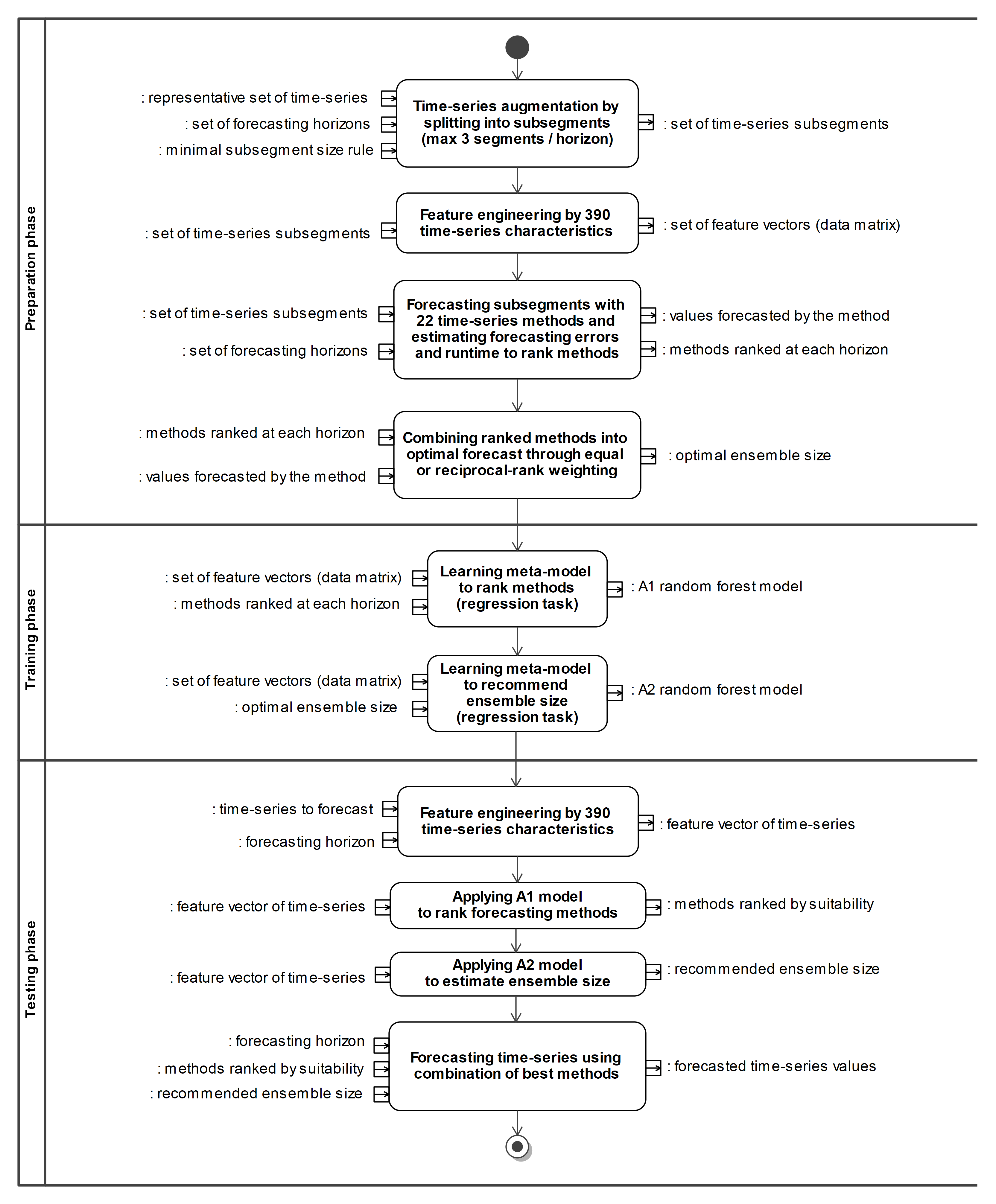
Figure 1: Methodology outline by unified modeling language activity diagram: input (left hand side) and output (right hand side) artefacts are listed besides each action block and all process is split into 3 phases. To adhere to machine learning standards, we assure that due to performed cross-validation a set of time-series in the preparation and training phases do not mach time-series in the testing phase.

3.1 Time-series features

Table 1: Overview of time-series features for meta-learning: 130 time-series characteristics in total.

Feature set	Size	R package(-s) used // detailed list of feature names
catch22	22	catch22 // DN_HistogramMode_5, DN_HistogramMode_10, CO_f1ecac, CO_FirstMin_ac, CO_HistogramAMI_even_2_5, CO_trev_1_num, MD_hrv_classic_pnn40, SB_BinaryStats_mean_longstretch1, SB_TransitionMatrix_3ac_sumdiagcov, PD_PeriodicityWang_th0_01, CO_Embed2_Dist_tau_d_expfit_meandiff, IN_AutoMutualInfoStats_40_gaussian_fmmi, FC_LocalSimple_mean1_tauresrat, DN_OutlierInclude_p_001_mdrmd, DN_OutlierInclude_n_001_mdrmd, SP_Summaries_welch_rect_area_5_1, SB_BinaryStats_diff_longstretch0, SB_MotifThree_quantile_hh, SC_FluctAnal_2_rsrangefit_50_1_logi_prop_r1, SC_FluctAnal_2_dfa_50_1_2_logi_prop_r1, SP_Summaries_welch_rect_centroid, FC_LocalSimple_mean3_stderr
tsfeats	13	tsfeatures // stability, lumpiness, crossing.points.fraction, flat.spots.fraction, nonlinearity, ur.kpss, ur.pp, arch.lm, ACF1, ACF10.SS, ACF.seas, PACF10.SS, PACF.seas
stlfeats	12	tsfeatures // nperiods, seasonal_period, trend, spike, linearity, curvature, e_acf1, e_acf10, seasonal_strength, peak, trough, lambda
hctsa	13	tsfeatures // embed2_incircle_1, embed2_incircle_2, ac_9, firstmin_ac, trev_num, motiftwo_entro3, walker_propcross, std1st_der, boot_stationarity_fixed, boot_stationarity_ac2, histogram_mode_10, outlierinclude_mdrmd, first_acf_zero_crossing
heterogeneity, portmanteau	6	tsfeatures, WeightedPortTest // arch_acf, garch_acf, arch_r2, garch_r2, lag1.Ljung.Box, lagF.Ljung.Box
stationarity, normality	10	tseries, stats, nortest // ADF, KPSS.Level, KPSS.Trend, PP, ShapiroWilk, Lilliefors, AndersonDarling, Pearson, CramerVonMises, ShapiroFrancia
kurtosis, skewness, misc	11	PerformanceAnalytics // kurtosis.fisher, kurtosis.sample, skewness.fisher, skewness.sample, skewness.variability, skewness.volatility, skewness.kurtosis.ratio, misc.smoothing.index, misc.Kelly.ratio, misc.drowpdown.average.depth, misc.drowpdown.average.length
Hurst	17	PerformanceAnalytics, longmemo, tsfeatures, liftLRD, pracma, fractal // PerformanceAnalytics, Whittle, HaslettRaftery, lifting, pracma.Hs, pracma.Hrs, pracma.He, pracma.Hal, pracma.Ht, fractal.spectral.lag.window, fractal.spectral.wosa, fractal.spectral.multitaper, fractal.block.aggabs, fractal.block.higuchi, fractal.ACVF.beta, fractal.ACVF.alpha, fractal.ACVF.HG
fractality	7	fractaldim // HallWood, DCT, wavelet, variogram, madogram, rodogram, periodogram
entropy	9	TSEntropies, ForeCA // TSE.approximate, TSE.fast.sample, TSE.fast.approx, spectral.smoothF.wosa, spectral.smoothF.direct, spectral.smoothF.multitaper, spectral.smoothT.wosa, spectral.smoothT.direct, spectral.smoothT.multitaper
anomaly	10	pracma, anomalize // fraction.TukeyMAD, twitter.iqr.fraction, twitter.iqr.infraction.pos, twitter.iqr.fraction.pos, twitter.iqr.abs.last.pos, twitter.iqr.rel.last.pos, twitter.iqr.infraction.neg, twitter.iqr.fraction.neg, twitter.iqr.abs.last.neg, twitter.iqr.rel.last.neg

Feature engineering for assistant models consisted of pooling various known time-series characteristics into a collection of 130 features (see Table 1). Almost half of all features were previously introduced as state-of-the-art time-series features, available in R packages catch22 [Lubba et al., 2019], consisting of carefully selected 22 features, and tsfeatures [Hyndman et al., 2019], consisting of 42 features also used in FFORMA framework [Montero-Manso et al., 2018, Montero-Manso et al., 2020].

Seeking to extend characteristics of time-series we considered calculating features not only on the original data (orig), but also on the results of 2 transformations (diff and log):

• diff - first differences help to improve/achieve stationarity;

• log - logarithmic transform has variance stabilizing properties.

Note that log transformation here is not applied column-wise to the table with extracted features, but to the original time-series, which seeks to achieve a variance-stabilizing effect on the dynamics at hand. Calculating 130 features on 3 variants of time-series (orig, diff and log) results in a final set of 390 features, which are later used for building assistant meta-learners.

3.2 Forecasting models

Table 2: A selected pool of 22 base models for univariate time-series forecasting. Most models are statistical, except for NNAR and xgb, which are based on machine learning. The horizontal line separates a few simple models from the remaining complex ones.

Model	R package::function	Description
SNaive	forecast::snaive	Seasonal naïve method
LinTrend	forecast::tslm	Linear trend
LinTrendSeason	forecast::tslm	Linear trend with seasonal dummies
QuadTrend	forecast::tslm	Quadratic trend
QuadTrendSeason	forecast::tslm	Quadratic trend with seasonal dummies
TSB	tsintermittent::tsb	Teunter-Syntetos-Babai method (based upon Croston for intermittent demand) with optimized parameters [Kourentzes, 2014]
ARIMA	forecast::auto.arima	Autoregressive integrated moving average [Hyndman and Khandakar, 2008]
SARIMA	forecast::auto.arima	Seasonal autoregressive integrated moving average [Hyndman and Khandakar, 2008]
ETS	forecast::ets	Family of exponential smoothing state space models [Hyndman et al., 2002, Hyndman et al., 2008]
HoltWinters	stats::HoltWinters	Holt-Winters filtering with additive seasonality [Winters, 1960]
Theta	forecast::thetaf	Theta method - simple exponential smoothing with drif [Assimakopoulos and Nikolopoulos, 2000]
STL-ARIMA	forecast::stlm	ARIMA model on seasonal decomposition of time series [Cleveland et al., 1990]
STL-ETS	forecast::stlm	ETS model on seasonal decomposition of time series [Cleveland et al., 1990]
StructTS	stats::StructTS	Basic stuctural model - local trend with seasonality [Durbin and Koopman, 2012]
BATS	forecast::tbats	Exponential smoothing with Box-Cox transform, ARMA errors, trend and complex seasonality [Livera et al., 2011]
Prophet	prophet::prophet	Decomposable time series and generalized additive model with non-linear trends [Taylor and Letham, 2017]
NNAR	forecast::nnetar	Neural network with a hidden layer and lagged inputs [Hyndman and Athanasopoulos, 2018]
xgb-none	forecastxgb::xgbar	Extreme gradient boosting model with lagged inputs [Ellis, 2016]
xgb-decompose	forecastxgb::xgbar	Extreme gradient boosting model with lagged inputs and decomposition-based seasonal adjustment [Ellis, 2016]
thief-ARIMA	thief::thief	Temporal hierarchical approach with ARIMA at each level [Athanasopoulos et al., 2017]
thief-ETS	thief::thief	Temporal hierarchical approach with ETS at each level [Athanasopoulos et al., 2017]
thief-Theta	thief::thief	Temporal hierarchical approach with Theta at each level [Athanasopoulos et al., 2017]

A representative pool of 22 univariate time-series forecasting models was selected (see Table 2). The diversity of models to consider as a potential ensemble member varies from simple, such as the seasonal naive and linear trend, to complex BATS and Prophet models. However, most of them are statistical, except for machine learning approaches NNAR and xgb. Model implementations from 6 R packages were used, where parameters when creating a model on time-series training part were chosen automatically if model implementation had that capability.

3.3 Forecasting errors

After fitting the univariate time-series model on the training part, forecasting can be performed for a required number of steps ahead, i.e., forecasting horizon. Comparing forecasted values with ground truth allows evaluating how accurate the forecast was, and forecasting errors are used for this purpose. We estimate three absolute and three relative forecasting errors.

Absolute forecasting errors considered:

• RMSE - root mean squared error;

• MAE - mean absolute error;

• MDAE - median absolute error.

Relative forecasting errors considered:

• SMAPE - symmetric mean absolute percentage error;

• MAAPE - mean arctangent absolute percentage error [Kim and Kim, 2016];

• MASE - mean absolute scaled error [Hyndman and Koehler, 2006].

The final ranking of forecasting models was constructed by averaging individual rankings, obtained for each error type separately. After averaging out individual rankings, a faster model was given priority in the final ranking in case of ties. Incorporating absolute and relative errors into the final ranking allows us to sort out models more comprehensively without less bias towards a single type of error. Relative forecasting errors were also reported in experiments to compare the introduced approach to benchmark methods (Theta and Comb).

3.4 Meta-learner model

Meta-learner for our experiments was random forest (RF) [Breiman, 2001] regression machine learning model. RF is an ensemble of many (ntrees in total) CART (classification and regression tree) instances. Each CART is built on an independent bootstrap sample of the original dataset while selecting from a random subset (of size mtry) of features at each tree node. Fast RF implementation in R package ranger [Wright and Ziegler, 2017] was chosen, which, conveniently for the specifics of our assistants, allows us to always include some variables as candidates for a binary node split besides mtry randomly selected ones. Time-series features were left for random selection, but a few critical meta-information features were set to always.split.variables parameter. Meta-information features were forecasting horizon length and data type (daily, weekly or monthly). Additionally, A1 assistant included model name (first column in Table 2) and three dummy indicators on model capabilities such as seasonality, complexity, and decomposition.

RF size ntrees was fixed at 256, as recommended in literature [Oshiro et al., 2012, Probst and Boulesteix, 2017]. Classical RF should be composed of unpruned CART, allowing growing trees to maximal possible depth, corresponding to min.node.size=1 setting, but in our case min.node.size parameter was tuned together with mtry using Bayesian optimization in R package tuneRanger with 21 warm-up and 9 tuning iterations. The minimization objective for A1 assistant was the out-of-bag root mean squared logarithmic error - a variant of RMSE penalizing errors at lower values and achieving that prediction of best-ranked cases is more precise than of worse-ranked candidates. The minimization objective for the A2 assistant was a simple out-of-bag RMSE metric. Both being RF regression models, A1 could be nick-named as a ”ranker” whereas A2 as a ”capper” due to different tasks they are dedicated to. A1 ranks 22 forecasting models to find the best candidates for the time-series at hand, while A2 tries to propose an optimal size of forecasting ensemble, i.e., a number of best-ranked models to choose for forecast pooling.

Two variants of forecast pooling, namely, Simple (arithmetic average) and Weighted (weighted average), were evaluated for meta-learning. A1 assistant was identical in both variants, but A2 was constructed separately after evaluation of cumulative pooling of forecasts from the best A1-ranked univariate time-series models, where pooling was done either with equal weights or weights derived from reciprocal rank [Aiolfi and Timmermann, 2006].

4 M4-micro dataset

We excluded two monthly cases (ID=19700 and ID=19505) from an original M4 subset of 12563 micro-economic time-series due to the lack of dynamics. Among 12561 selected cases level of aggregation was as follows: 1476 daily, 112 weekly, and 10973 monthly. All selected cases were pre-processed by segmenting them properly into train/test splits at several forecasting horizons. Forecasting horizons with a varying number of steps ahead were considered: 15, 30, 90, 180, 365, and 730 days for daily data; 4, 13, 26, 52, and 104 weeks for weekly data; 6, 12, 24, 60, and 120 months for monthly data.

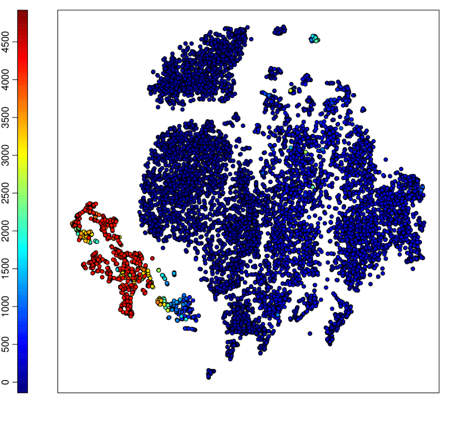
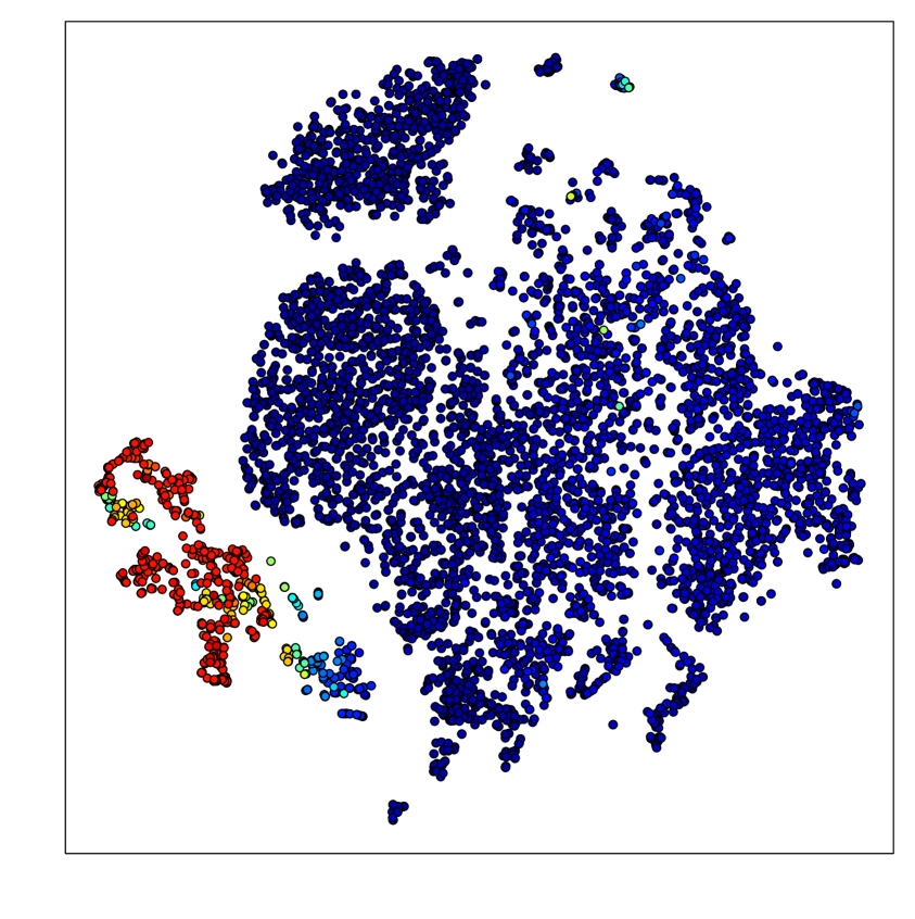
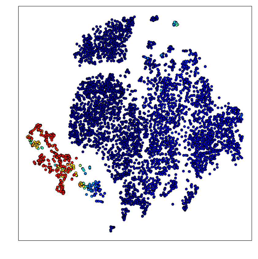
Figure 2: Visualization of M4-micro dataset by 2D $t$-SNE projection of time-series features: full sample of 12561 time-series (left) and result after balanced sampling into 2 cross-validation folds, containing 6281 (center) and 6280 (right) time-series. Color of the point denotes the length of time-series. Note that to avoid any informational leakage splitting into 2 cross-validation folds was done for the original dataset before proceeding with expansions.

Concerned with specifics of time-series representation space [Spiliotis et al., 2020] and to avoid potential concept drift situation if meta-learners are built using random sub-spaces, we split the dataset by performing a stratified 2-fold cross-validation (2-fold CV) carefully. Stratification is done here by an efficient balanced sampling [Deville and Tillé, 2004] on 3D $t$-SNE [van der Maaten, 2014] projection of time-series features, which allows splitting the time-series dataset into two equally-sized parts where each part covers the overall representation space of the initial dataset. The result of such stratification is visualized in Fig. 2 with resulting CV folds depicted after 2D $t$-SNE projection.

Table 3: Expanding M4 micro dataset for benchmarking and augmentation. The expansion was performed by segmenting each time-series into various train/test splits, fulfilling the 80/20 heuristic. Heuristic ensures that the amount of data available for time-series model training is at least four times larger than for testing. The amount of data for estimating forecasting error of the meta-learner solution is defined by the forecasting horizon. Full sample for benchmarking at the smallest forecasting horizon consists of 12561 time-series, visualized on the left of Fig. 2.

Horizon	Initial expansion for benchmarking			Final expansion for augmentation
	Full sample	CV fold 1	CV fold 2	Full sample	CV fold 1	CV fold 2
15 days	1476	736	740	4374	2178	2196
30 days	1443	720	723	4201	2100	2101
90 days	1335	667	668	3699	1853	1846
180 days	1181	593	588	3313	1661	1652
365 days	1047	524	523	2693	1346	1347
730 days	780	389	391	780	389	391
$\sum$	7262	3629	3633	19060	9527	9533
4 weeks	112	58	54	206	106	100
13 weeks	112	58	54	206	106	100
26 weeks	47	24	23	141	72	69
52 weeks	47	24	23	119	60	59
104 weeks	36	18	18	76	40	36
$\sum$	354	182	172	748	384	364
6 months	10973	5486	5487	32904	16452	16452
12 months	10973	5486	5487	22317	11166	11151
24 months	5574	2792	2782	14110	7055	7055
60 months	3432	1713	1719	3630	1813	1817
120 months	65	31	34	77	33	44
$\sum$	31017	15508	15509	73038	36519	36519
$\sum$	38633	19319	19314	92846	46430	46416

Time-series expansion by segmenting data into several train/test hold-out splits was done as follows. Initially, we expand a set of time-series from 12561 to 38633 (see initial expansion in Table 3) to be able to test various forecasting horizons. Then we increase the amount of time-series from 38633 to 92846 (see final expansion in Table 3) by considering additional splitting time-series in half to be able to train meta-learners on more data. Initial expansion was carried out to benchmark various forecasting horizons, and only recent data was split-off for testing. In contrast, final expansion was considered as a way of data augmentation to harvest more training data for meta-learners. Besides initial expansion, extra two splits were done where possible - hold-out on older and newer halves of time-series. Following the recommendation of [Cerqueira et al., 2020] for using an out-of-sample hold-out split in multiple testing periods, we consider 80/20 as a sufficient train/test ratio. After leaving out the last observations for testing (based on the forecasting horizon’s length), if the amount of the training data drops down below 80% we refuse to segment time-series.

5 Experimental results

The forecasting experiment was performed using 2-fold CV by creating assistants on CV fold 1 of final expansion and testing success of assistant-recommended forecasting ensemble on CV fold 2 of initial expansion and vice versa. Besides forecasting using the proposed approach, benchmark methods Theta and Comb were used on initial expansion, and relative forecasting errors were calculated for comparison.

Table 4: Forecasting results according to SMAPE forecasting error. $\sum$ denotes results over all horizons, the best result for each row is formatted in italic-bold.

Horizon	Theta	Comb	Simple	Weighted
15 days	2.507 $\pm$ 0.152	2.511 $\pm$ 0.146	2.326 $\pm$ 0.145	2.332 $\pm$ 0.153
30 days	3.354 $\pm$ 0.277	3.340 $\pm$ 0.282	3.233 $\pm$ 0.287	3.229 $\pm$ 0.286
90 days	5.587 $\pm$ 0.312	5.576 $\pm$ 0.318	5.060 $\pm$ 0.310	5.064 $\pm$ 0.310
180 days	8.296 $\pm$ 0.444	8.565 $\pm$ 0.452	7.298 $\pm$ 0.438	7.282 $\pm$ 0.438
365 days	17.258 $\pm$ 0.919	17.304 $\pm$ 0.895	14.098 $\pm$ 0.829	14.145 $\pm$ 0.828
730 days	18.270 $\pm$ 1.003	19.052 $\pm$ 1.042	16.396 $\pm$ 0.974	16.395 $\pm$ 0.991
$\sum$	8.003 $\pm$ 0.245	8.133 $\pm$ 0.248	7.026 $\pm$ 0.225	7.031 $\pm$ 0.226
4 weeks	9.483 $\pm$ 1.152	9.653 $\pm$ 1.198	7.941 $\pm$ 1.024	7.867 $\pm$ 1.000
13 weeks	9.365 $\pm$ 1.130	8.910 $\pm$ 1.047	8.481 $\pm$ 1.076	8.637 $\pm$ 1.222
26 weeks	8.895 $\pm$ 4.395	8.594 $\pm$ 4.404	8.184 $\pm$ 4.378	8.092 $\pm$ 4.371
52 weeks	13.340 $\pm$ 4.619	12.575 $\pm$ 4.036	10.763 $\pm$ 3.519	10.922 $\pm$ 3.784
104 weeks	17.452 $\pm$ 5.277	18.198 $\pm$ 6.037	16.273 $\pm$ 4.767	16.008 $\pm$ 4.855
$\sum$	10.690 $\pm$ 1.126	10.534 $\pm$ 1.127	9.366 $\pm$ 1.010	9.374 $\pm$ 1.041
6 months	12.150 $\pm$ 0.278	12.147 $\pm$ 0.286	9.158 $\pm$ 0.214	9.096 $\pm$ 0.212
12 months	12.183 $\pm$ 0.246	12.874 $\pm$ 0.269	10.479 $\pm$ 0.222	10.420 $\pm$ 0.220
24 months	9.544 $\pm$ 0.352	9.325 $\pm$ 0.353	8.451 $\pm$ 0.327	8.486 $\pm$ 0.333
60 months	12.724 $\pm$ 0.604	14.780 $\pm$ 0.740	11.617 $\pm$ 0.583	11.449 $\pm$ 0.567
120 months	15.051 $\pm$ 5.820	13.656 $\pm$ 4.244	10.798 $\pm$ 3.371	10.650 $\pm$ 3.329
$\sum$	11.763 $\pm$ 0.161	12.192 $\pm$ 0.174	9.774 $\pm$ 0.140	9.719 $\pm$ 0.139
$\sum$	11.047 $\pm$ 0.139	11.414 $\pm$ 0.149	9.254 $\pm$ 0.121	9.210 $\pm$ 0.120

Results by SMAPE (see Table 4) demonstrate that both Simple and Weighted variants of meta-learning outperform Theta and Comb techniques. Weighted slightly outperformed Simple variant for more than half (10 out of 16) horizons and also overall (see the last row in Table 4).

Table 5: Forecasting results according to MAAPE forecasting error. $\sum$ denotes results over all horizons, the best result for each row is formatted in italic-bold.

Horizon	Theta	Comb	Simple	Weighted
15 days	2.520 $\pm$ 0.151	2.536 $\pm$ 0.153	2.335 $\pm$ 0.148	2.335 $\pm$ 0.153
30 days	3.312 $\pm$ 0.268	3.296 $\pm$ 0.269	3.185 $\pm$ 0.273	3.183 $\pm$ 0.272
90 days	5.538 $\pm$ 0.316	5.526 $\pm$ 0.318	5.033 $\pm$ 0.317	5.036 $\pm$ 0.317
180 days	8.047 $\pm$ 0.433	8.366 $\pm$ 0.444	7.161 $\pm$ 0.434	7.142 $\pm$ 0.434
365 days	15.431 $\pm$ 0.783	15.538 $\pm$ 0.772	13.132 $\pm$ 0.766	13.165 $\pm$ 0.765
730 days	17.696 $\pm$ 0.971	17.989 $\pm$ 0.975	16.306 $\pm$ 0.993	16.286 $\pm$ 1.000
$\sum$	7.622 $\pm$ 0.226	7.719 $\pm$ 0.228	6.842 $\pm$ 0.218	6.842 $\pm$ 0.219
4 weeks	8.750 $\pm$ 1.027	8.856 $\pm$ 1.061	7.570 $\pm$ 0.953	7.514 $\pm$ 0.938
13 weeks	9.475 $\pm$ 1.146	8.896 $\pm$ 1.057	8.636 $\pm$ 1.142	8.717 $\pm$ 1.207
26 weeks	8.471 $\pm$ 4.175	8.233 $\pm$ 4.190	7.945 $\pm$ 4.213	7.849 $\pm$ 4.208
52 weeks	12.084 $\pm$ 3.451	11.620 $\pm$ 3.374	10.231 $\pm$ 3.223	10.270 $\pm$ 3.320
104 weeks	15.683 $\pm$ 3.885	16.119 $\pm$ 4.218	15.251 $\pm$ 3.890	14.979 $\pm$ 3.921
$\sum$	10.090 $\pm$ 0.955	9.891 $\pm$ 0.962	9.091 $\pm$ 0.938	9.064 $\pm$ 0.949
6 months	11.059 $\pm$ 0.242	10.983 $\pm$ 0.243	8.892 $\pm$ 0.207	8.840 $\pm$ 0.206
12 months	12.239 $\pm$ 0.244	13.203 $\pm$ 0.273	10.648 $\pm$ 0.224	10.593 $\pm$ 0.223
24 months	9.119 $\pm$ 0.320	8.906 $\pm$ 0.319	8.190 $\pm$ 0.306	8.200 $\pm$ 0.307
60 months	12.500 $\pm$ 0.601	13.512 $\pm$ 0.601	11.330 $\pm$ 0.556	11.197 $\pm$ 0.548
120 months	11.883 $\pm$ 3.194	11.499 $\pm$ 2.941	9.389 $\pm$ 2.538	9.341 $\pm$ 2.539
$\sum$	11.289 $\pm$ 0.151	11.676 $\pm$ 0.158	9.658 $\pm$ 0.136	9.607 $\pm$ 0.136
$\sum$	10.589 $\pm$ 0.129	10.916 $\pm$ 0.135	9.123 $\pm$ 0.118	9.082 $\pm$ 0.117

Results by MAAPE (see Table 5) demonstrate that both Simple and Weighted variants of meta-learning outperform Theta and Comb techniques. Weighted slightly outperformed Simple variant for more than half (11 out of 16) horizons and also overall (see the last row in Table 5).

Table 6: Forecasting results according to MASE forecasting error. $\sum$ denotes results over all horizons, the best result for each row is formatted in italic-bold.

Horizon	Theta	Comb	Simple	Weighted
115 days	1.047 $\pm$ 0.050	1.056 $\pm$ 0.055	0.963 $\pm$ 0.046	0.964 $\pm$ 0.049
30 days	1.365 $\pm$ 0.076	1.362 $\pm$ 0.077	1.311 $\pm$ 0.081	1.310 $\pm$ 0.081
90 days	2.245 $\pm$ 0.106	2.239 $\pm$ 0.107	1.997 $\pm$ 0.102	1.996 $\pm$ 0.101
180 days	3.265 $\pm$ 0.200	3.334 $\pm$ 0.200	2.910 $\pm$ 0.202	2.904 $\pm$ 0.202
365 days	5.987 $\pm$ 0.309	6.132 $\pm$ 0.320	5.053 $\pm$ 0.301	5.060 $\pm$ 0.300
730 days	7.676 $\pm$ 0.521	7.798 $\pm$ 0.517	6.747 $\pm$ 0.484	6.761 $\pm$ 0.504
$\sum$	3.115 $\pm$ 0.098	3.161 $\pm$ 0.099	2.750 $\pm$ 0.091	2.751 $\pm$ 0.092
4 weeks	0.579 $\pm$ 0.077	0.592 $\pm$ 0.084	0.480 $\pm$ 0.070	0.475 $\pm$ 0.068
13 weeks	0.486 $\pm$ 0.052	0.476 $\pm$ 0.058	0.426 $\pm$ 0.047	0.432 $\pm$ 0.051
26 weeks	0.681 $\pm$ 0.324	0.680 $\pm$ 0.350	0.622 $\pm$ 0.347	0.599 $\pm$ 0.340
52 weeks	0.993 $\pm$ 0.299	0.967 $\pm$ 0.308	0.821 $\pm$ 0.282	0.806 $\pm$ 0.286
104 weeks	1.713 $\pm$ 0.731	1.689 $\pm$ 0.701	1.564 $\pm$ 0.729	1.587 $\pm$ 0.753
$\sum$	0.733 $\pm$ 0.103	0.728 $\pm$ 0.103	0.637 $\pm$ 0.101	0.635 $\pm$ 0.103
6 months	0.642 $\pm$ 0.011	0.637 $\pm$ 0.011	0.513 $\pm$ 0.010	0.511 $\pm$ 0.010
12 months	0.730 $\pm$ 0.013	0.750 $\pm$ 0.014	0.625 $\pm$ 0.012	0.622 $\pm$ 0.012
24 months	1.153 $\pm$ 0.029	1.118 $\pm$ 0.029	0.977 $\pm$ 0.027	0.977 $\pm$ 0.027
60 months	1.986 $\pm$ 0.099	2.428 $\pm$ 0.131	1.919 $\pm$ 0.221	1.827 $\pm$ 0.130
120 months	4.217 $\pm$ 1.153	4.025 $\pm$ 1.120	3.162 $\pm$ 0.982	3.144 $\pm$ 0.989
$\sum$	0.921 $\pm$ 0.015	0.968 $\pm$ 0.018	0.797 $\pm$ 0.026	0.785 $\pm$ 0.017
$\sum$	1.332 $\pm$ 0.023	1.378 $\pm$ 0.025	1.163 $\pm$ 0.028	1.153 $\pm$ 0.023

Results by MASE (see Table 6) demonstrate that both Simple and Weighted variants of meta-learning outperform Theta and Comb techniques. Weighted slightly outperformed Simple variant for more than half (12 out of 16) horizons and also overall (see the last row in Table 5).

Forecasting errors showed an expected and consistent tendency to increase together with increasing forecasting horizon length. Interestingly, MASE errors were the lowest overall for weekly whereas SMAPE and MAAPE for daily data. To summarize over all data types and horizons: among benchmark methods, Theta tends to outperform Comb slightly, and meta-learning approaches win over both benchmarks with the Weighted variant as the best.

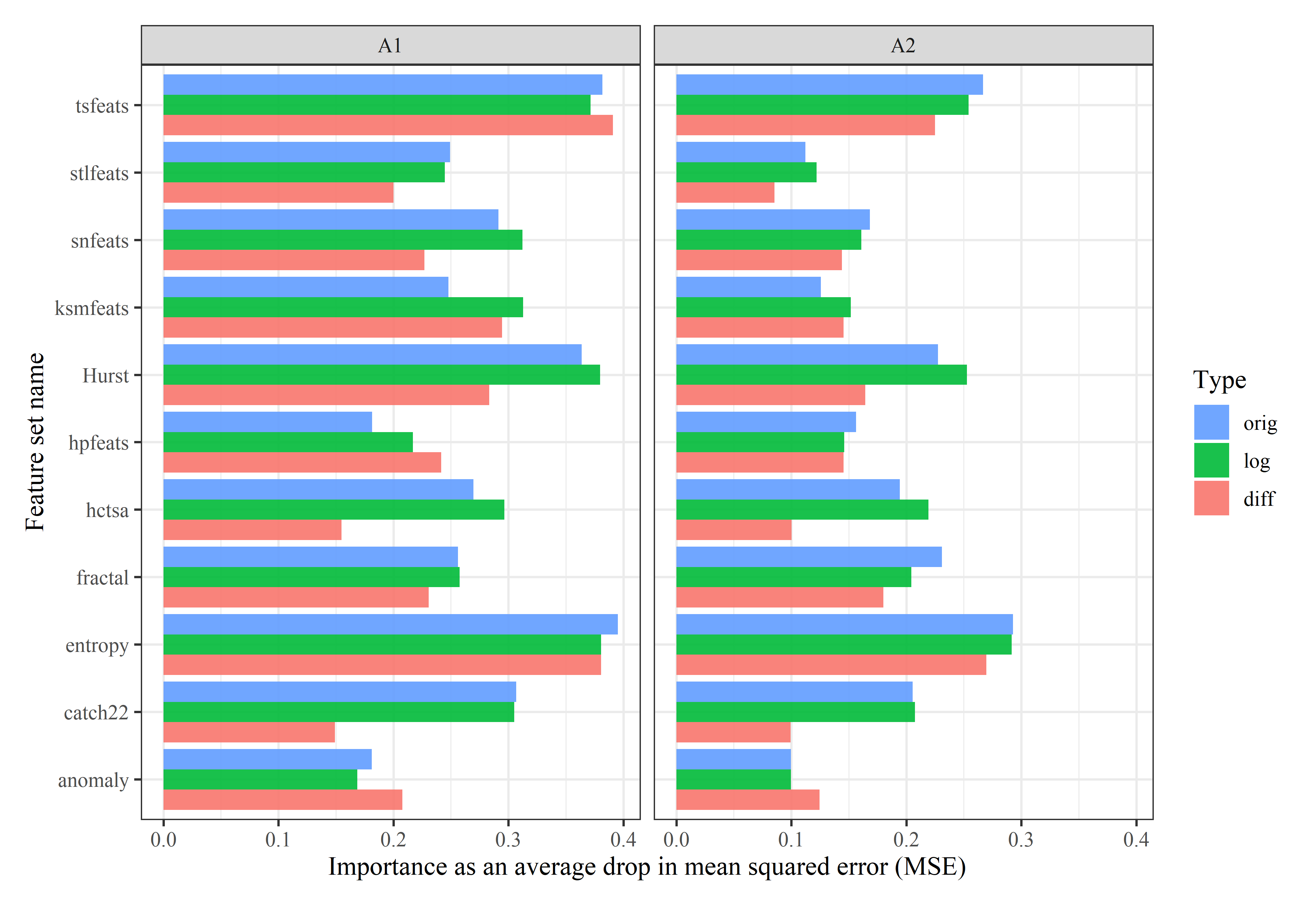
Figure 3: Permutation-based variable importance from meta-learner – a random forest regression model: A1 (left) and A2 (right) assistants.

We have measured the prognostic usefulness of time-series characteristics for additional insights into meta-learners by calculating permutation-based variable importance for a random forest model built on a full M4-micro dataset. Variable importance was measured as a drop in mean squared error of the random forest regression model after permuting each feature, i.e., how strongly distorting ties between a feature in question and a target affects the model’s accuracy. Feature sets had several features, so their corresponding individual importance estimates were averaged for a fair comparison and are reported in Fig. 3. From comparison it can be noticed that both transformations (log and diff) besides original time-series were useful, with the exception of diff transformation for hctsa and catch22 features. Interestingly, the pre-processing of time-series by log transformation was highly useful for most feature sets. The best feature sets for meta-learning tasks were entropy, tsfeats, and Hurst. Among the least useful feature sets anomaly could be considered for removal.

Since we did not use the full M4 dataset (just 12.561% from the entire dataset of 100000 time-series) and tested much more forecasting horizons, it would be improper to compare SMAPE and MASE errors directly to M4 competition results. Nonetheless, the measure ”% improvement of method over the benchmark” from Table 4 in [Makridakis et al., 2020] could lend itself for comparison with the winner of M4 competition - Smyl (Uber) reached an improvement of 9.4% in SMAPE and 7.7% in MASE over baseline Comb method. Our Weighted variant here demonstrated an improvement of 19.3% in SMAPE and 16.3% in MASE.

6 Conclusions

Extensive evaluation of the proposed meta-learning approach on micro-economic time-series from M4 competition demonstrated that meta-learning could outperform benchmark methods Theta and Comb. The best performance was achieved by pooling forecasts from assistant-recommended univariate time-series models using weighted average with weights corresponding to reciprocal rank. Lower forecasting errors were obtained using a weighted variant of forecasting ensemble over the Theta method: 9.21% versus 11.05% by SMAPE, 9.08% versus 10.59% by MAAPE, 1.15 versus 1.33 by MASE. The regression meta-learner model was more successful and had a better out-of-bag fit for A1 than for A2 assistant. All transformations were found to be useful for feature engineering and the most effective time-series characteristics for meta-learner were entropy, tsfeats, and Hurst feature sets. Considering a more extensive set of time-series data for meta-learning and exploring automatic feature engineering’s usefulness using sequence-to-sequence auto-encoder would be exciting directions for further research.

Data Availability Statement

This study was a re-analysis of existing data, which is publicly available in:

• R packages M4comp and M4comp2018

• Kaggle platform

• Zenodo platform:

  • M4 Daily Dataset [Godahewa et al., 2020a]

  • M4 Weekly Dataset [Godahewa et al., 2020c]

  • M4 Monthly Dataset [Godahewa et al., 2020b]

References

- Aiolfi and Timmermann, 2006 Aiolfi, M. and Timmermann, A. (2006). Persistence in forecasting performance and conditional combination strategies. Journal of Econometrics, 135(1-2):31–53. doi:10.1016/j.jeconom.2005.07.015.
- Ali et al., 2018 Ali, A. R., Gabrys, B., and Budka, M. (2018). Cross-domain meta-learning for time-series forecasting. Procedia Computer Science, 126:9–18. doi:10.1016/j.procs.2018.07.204.
- Assimakopoulos and Nikolopoulos, 2000 Assimakopoulos, V. and Nikolopoulos, K. (2000). The theta model: a decomposition approach to forecasting. International Journal of Forecasting, 16(4):521–530. doi:10.1016/S0169-2070(00)00066-2.
- Athanasopoulos et al., 2017 Athanasopoulos, G., Hyndman, R. J., Kourentzes, N., and Petropoulos, F. (2017). Forecasting with temporal hierarchies. European Journal of Operational Research, 262(1):60–74. doi:10.1016/j.ejor.2017.02.046.
- Bauer et al., 2020 Bauer, A., Züfle, M., Grohmann, J., Schmitt, N., Herbst, N., and Kounev, S. (2020). An automated forecasting framework based on method recommendation for seasonal time series. In Proceedings of the ACM/SPEC International Conference on Performance Engineering. ACM. doi:10.1145/3358960.3379123.
- Breiman, 2001 Breiman, L. (2001). Random forests. Machine Learning, 45:5–32. doi:10.1023/A:1010933404324.
- Cerqueira et al., 2020 Cerqueira, V., Torgo, L., and Mozetič, I. (2020). Evaluating time series forecasting models: an empirical study on performance estimation methods. Machine Learning. doi:10.1007/s10994-020-05910-7.
- Clemen, 1989 Clemen, R. T. (1989). Combining forecasts: A review and annotated bibliography. International Journal of Forecasting, 5(4):559 –583. doi:10.1016/0169-2070(89)90012-5.
- Cleveland et al., 1990 Cleveland, R. B., Cleveland, W. S., McRae, J. E., and Terpenning, I. (1990). STL: A seasonal-trend decomposition procedure based on loess (with discussion). Journal of Official Statistics, 6:3–73.
- Collopy and Armstrong, 1992 Collopy, F. and Armstrong, J. S. (1992). Rule-based forecasting: Development and validation of an expert systems approach to combining time series extrapolations. Management Science, 38(10):1394–1414. doi:10.1287/mnsc.38.10.1394.
- Deville and Tillé, 2004 Deville, J.-C. and Tillé, Y. (2004). Efficient balanced sampling: The cube method. Biometrika, 91(4):893–912. doi:10.1093/biomet/91.4.893.
- Durbin and Koopman, 2012 Durbin, J. and Koopman, S. J. (2012). Time Series Analysis by State Space Methods. Oxford University Press. doi:10.1093/acprof:oso/9780199641178.001.0001.
- Ellis, 2016 Ellis, P. (2016). Timeseries forecasting using extreme gradient boosting. http://freerangestats.info/blog/2016/11/06/forecastxgb.
- Godahewa et al., 2020a Godahewa, R., Bergmeir, C., and Webb, G. (2020a). M4 daily dataset. doi:10.5281/ZENODO.3898361.
- Godahewa et al., 2020b Godahewa, R., Bergmeir, C., and Webb, G. (2020b). M4 monthly dataset. doi:10.5281/ZENODO.3898380.
- Godahewa et al., 2020c Godahewa, R., Bergmeir, C., and Webb, G. (2020c). M4 weekly dataset. doi:10.5281/ZENODO.3898376.
- Hansen and Salamon, 1990 Hansen, L. K. and Salamon, P. (1990). Neural network ensembles. IEEE Transactions on Pattern Analysis and Machine Intelligence, 12(10):993–1001. doi:10.1109/34.58871.
- Hendry and Clements, 2004 Hendry, D. F. and Clements, M. P. (2004). Pooling of forecasts. The Econometrics Journal, 7(1):1–31. doi:10.1111/j.1368-423X.2004.00119.x.
- Hyndman and Athanasopoulos, 2018 Hyndman, R. and Athanasopoulos, G. (2018). Forecasting: Principles and Practice, chapter Neural network models, page 11.3. OTexts, 2nd edition. https://otexts.com/fpp2/nnetar.html#nnetar.
- Hyndman and Khandakar, 2008 Hyndman, R. and Khandakar, Y. (2008). Automatic time series forecasting: The forecast package for r. Journal of Statistical Software, Articles, 27(3):1–22. doi:10.18637/jss.v027.i03.
- Hyndman et al., 2008 Hyndman, R., Koehler, A., Ord, K., and Snyder, R. (2008). Forecasting with Exponential Smoothing. Springer Berlin Heidelberg. doi:10.1007/978-3-540-71918-2.
- Hyndman et al., 2019 Hyndman, R., Wang, E., Kang, Y., Talagala, T., and Yang, Y. (2019). tsfeatures: Time series feature extraction. https://github.com/robjhyndman/tsfeatures/.
- Hyndman, 2010 Hyndman, R. J. (2010). Business forecasting methods. In Lovric, M., editor, International Encyclopedia of Statistical Science, page 185–187. Springer, Berlin, Heidelberg. doi:10.1007/978-3-642-04898-2˙156.
- Hyndman and Koehler, 2006 Hyndman, R. J. and Koehler, A. B. (2006). Another look at measures of forecast accuracy. International Journal of Forecasting, 22(4):679–688. doi:10.1016/j.ijforecast.2006.03.001.
- Hyndman et al., 2002 Hyndman, R. J., Koehler, A. B., Snyder, R. D., and Grose, S. (2002). A state space framework for automatic forecasting using exponential smoothing methods. International Journal of Forecasting, 18(3):439–454. doi:10.1016/S0169-2070(01)00110-8.
- Kim and Kim, 2016 Kim, S. and Kim, H. (2016). A new metric of absolute percentage error for intermittent demand forecasts. International Journal of Forecasting, 32(3):669–679. doi:10.1016/j.ijforecast.2015.12.003.
- Kolassa, 2011 Kolassa, S. (2011). Combining exponential smoothing forecasts using Akaike weights. International Journal of Forecasting, 27(2):238–251. doi:10.1016/j.ijforecast.2010.04.006.
- Kourentzes, 2014 Kourentzes, N. (2014). On intermittent demand model optimisation and selection. International Journal of Production Economics, 156:180–190. doi:10.1016/j.ijpe.2014.06.007.
- Lemke and Gabrys, 2010 Lemke, C. and Gabrys, B. (2010). Meta-learning for time series forecasting and forecast combination. Neurocomputing, 73:2006–2016. doi:10.1016/j.neucom.2009.09.020.
- Livera et al., 2011 Livera, A. M. D., Hyndman, R. J., and Snyder, R. D. (2011). Forecasting time series with complex seasonal patterns using exponential smoothing. Journal of the American Statistical Association, 106(496):1513–1527. doi:10.1198/jasa.2011.tm09771.
- Lubba et al., 2019 Lubba, C. H., Sethi, S. S., Knaute, P., Schultz, S. R., Fulcher, B. D., and Jones, N. S. (2019). catch22: CAnonical time-series CHaracteristics. Data Mining and Knowledge Discovery, 33(6):1821–1852. doi:10.1007/s10618-019-00647-x.
- Ma and Fildes, 2021 Ma, S. and Fildes, R. (2021). Retail sales forecasting with meta-learning. European Journal of Operational Research, 288(1):111–128. doi:10.1016/j.ejor.2020.05.038.
- Makridakis and Hibon, 2000 Makridakis, S. and Hibon, M. (2000). The m3-competition: results, conclusions and implications. International Journal of Forecasting, 16(4):451–476. The M3-Competition, doi:10.1016/S0169-2070(00)00057-1.
- Makridakis et al., 2018 Makridakis, S., Spiliotis, E., and Assimakopoulos, V. (2018). The m4 competition: Results, findings, conclusion and way forward. International Journal of Forecasting, 34(4):802–808. doi:10.1016/j.ijforecast.2018.06.001.
- Makridakis et al., 2020 Makridakis, S., Spiliotis, E., and Assimakopoulos, V. (2020). The m4 competition: 100,000 time series and 61 forecasting methods. International Journal of Forecasting, 36(1):54–74. doi:10.1016/j.ijforecast.2019.04.014.
- Meade, 2000 Meade, N. (2000). Evidence for the selection of forecasting methods. Journal of Forecasting, 19(6):515–535. doi:10.1002/1099-131X(200011)19:6¡515::AID-FOR754¿3.0.CO;2-7.
- Montero-Manso et al., 2018 Montero-Manso, P., Athanasopoulos, G., Hyndman, R. J., and Talagala, T. S. (2018). Fforma: Feature-based forecast model averaging. resreport 19/18, Department of Econometrics and Business Statistics, Monash Business School, Monash University. Working Paper Series.
- Montero-Manso et al., 2020 Montero-Manso, P., Athanasopoulos, G., Hyndman, R. J., and Talagala, T. S. (2020). FFORMA: Feature-based forecast model averaging. International Journal of Forecasting, 36(1):86–92. doi:10.1016/j.ijforecast.2019.02.011.
- Oliveira and Torgo, 2015 Oliveira, M. and Torgo, L. (2015). Ensembles for time series forecasting. In Phung, D. and Li, H., editors, Proceedings of Machine Learning Research, volume 39, pages 360–370, Nha Trang City, Vietnam. PMLR. http://proceedings.mlr.press/v39/oliveira14.html.
- Oshiro et al., 2012 Oshiro, T. M., Perez, P. S., and Baranauskas, J. A. (2012). How many trees in a random forest? In Machine Learning and Data Mining in Pattern Recognition, pages 154–168. Springer Berlin Heidelberg. doi:10.1007/978-3-642-31537-4˙13.
- Petropoulos et al., 2014 Petropoulos, F., Makridakis, S., Assimakopoulos, V., and Nikolopoulos, K. (2014). ‘horses for courses’ in demand forecasting. European Journal of Operational Research, 237(1):152–163. doi:10.1016/j.ejor.2014.02.036.
- Probst and Boulesteix, 2017 Probst, P. and Boulesteix, A.-L. (2017). To tune or not to tune the number of trees in random forest. Journal of Machine Learning Research, 18(1):6673–6690. https://www.jmlr.org/papers/v18/17-269.html.
- Reid, 1972 Reid, D. (1972). A comparison of forecasting techniques on economic time series. Forecasting in Action. Operational Research Society and the Society for Long Range Planning.
- Rokach, 2006 Rokach, L. (2006). Decomposition methodology for classification tasks: a meta decomposer framework. Pattern Analysis and Applications, 9:257–271. doi:10.1007/s10044-006-0041-y.
- Smith and Wallis, 2009 Smith, J. and Wallis, K. F. (2009). A simple explanation of the forecast combination puzzle. Oxford Bulletin of Economics and Statistics, 71(3):331–355. doi:10.1111/j.1468-0084.2008.00541.x.
- Spiliotis et al., 2020 Spiliotis, E., Kouloumos, A., Assimakopoulos, V., and Makridakis, S. (2020). Are forecasting competitions data representative of the reality? International Journal of Forecasting, 36(1):37–53. doi:10.1016/j.ijforecast.2018.12.007.
- Talagala et al., 2018 Talagala, T. S., Hyndman, R. J., and Athanasopoulos, G. (2018). Meta-learning how to forecast time series. resreport 6/18, Department of Econometrics and Business Statistics, Monash Business School, Monash University. Working Paper Series.
- Taylor and Letham, 2017 Taylor, S. J. and Letham, B. (2017). Forecasting at scale. PeerJ Preprints, 5:e3190v2. doi:10.7287/peerj.preprints.3190v2.
- Timmermann, 2006 Timmermann, A. (2006). Forecast combinations. In Elliott, G., Granger, C. W. J., and Timmermann, A., editors, Handbook of Economic Forecasting, volume 1, chapter 4, pages 135–196. Elsevier. doi:10.1016/S1574-0706(05)01004-9.
- van der Maaten, 2014 van der Maaten, L. (2014). Accelerating t-SNE using tree-based algorithms. Journal of Machine Learning Research, 15(93):3221–3245. http://jmlr.org/papers/v15/vandermaaten14a.html.
- Wacker and Lummus, 2002 Wacker, J. G. and Lummus, R. R. (2002). Sales forecasting for strategic resource planning. International Journal of Operations & Production Management, 22(9):1014–1031. doi:10.1108/01443570210440519.
- Wang et al., 2009 Wang, X., Smith-Miles, K., and Hyndman, R. (2009). Rule induction for forecasting method selection: Meta-learning the characteristics of univariate time series. Neurocomputing, 72:2581–2594. doi:10.1016/j.neucom.2008.10.017.
- Winters, 1960 Winters, P. R. (1960). Forecasting sales by exponentially weighted moving averages. Management Science, 6(3):324–342. doi:10.1287/mnsc.6.3.324.
- Wright and Ziegler, 2017 Wright, M. and Ziegler, A. (2017). ranger: A fast implementation of random forests for high dimensional data in c++ and r. Journal of Statistical Software, Articles, 77(1):1–17. doi:10.18637/jss.v077.i01.
- Zang et al., 2014 Zang, W., Zhang, P., Zhou, C., and Guo, L. (2014). Comparative study between incremental and ensemble learning on data streams: Case study. Journal of Big Data, 1(1):1–5. doi:10.1186/2196-1115-1-5.
- Zou and Yang, 2004 Zou, H. and Yang, Y. (2004). Combining time series models for forecasting. International Journal of Forecasting, 20(1):69–84. doi:10.1016/s0169-2070(03)00004-9.
- Zuefle et al., 2019 Zuefle, M., Bauer, A., Lesch, V., Krupitzer, C., Herbst, N., Kounev, S., and Curtef, V. (2019). Autonomic forecasting method selection: Examination and ways ahead. In 2019 IEEE International Conference on Autonomic Computing (ICAC). IEEE. doi:10.1109/icac.2019.00028.