Qubit-excitation-based adaptive variational quantum eigensolver

I Abstract

Molecular simulations with the variational quantum eigensolver (VQE) are a promising application for emerging noisy intermediate-scale quantum computers. Constructing accurate molecular ansätze that are easy to optimize and implemented by shallow quantum circuits is crucial for the successful implementation of such simulations. Ansätze are, generally, constructed as series of fermionic-excitation evolutions. Instead, we demonstrate the usefulness of constructing ansätze with “qubit-excitation evolutions”, which, contrary to fermionic excitation evolutions, obey “qubit commutation relations”. We show that qubit excitation evolutions, despite the lack of some of the physical features of fermionic excitation evolutions, accurately construct ansätze, while requiring asymptotically fewer gates. Utilizing qubit excitation evolutions, we introduce the qubit-excitation-based adaptive (QEB-ADAPT)-VQE protocol. The QEB-ADAPT-VQE is a modification of the ADAPT-VQE that performs molecular simulations using a problem-tailored ansatz, grown iteratively by appending evolutions of qubit excitation operators. By performing classical numerical simulations for small molecules, we benchmark the QEB-ADAPT-VQE, and compare it against the original fermionic-ADAPT-VQE and the qubit-ADAPT-VQE. In terms of circuit efficiency and convergence speed, we demonstrate that the QEB-ADAPT-VQE outperforms the qubit-ADAPT-VQE, which to our knowledge was the previous most circuit-efficient scalable VQE protocol for molecular simulations.

II Introduction

Quantum computers are anticipated to enable simulations of quantum systems more efficiently and accurately than classical computers Benioff (1980); Feynman (1999). A promising algorithm to perform this task on emerging noisy intermediate-scale quantum (NISQ) Preskill (2018); Arute et al. (2019); Elfving et al. (2020) computers is the variational quantum eigensolver (VQE) McArdle et al. (2020); McClean et al. (2016); Cerezo et al. (2020a); O’Malley et al. (2016); Wang et al. (2019); Arute et al. (2020); Gonthier et al. (2020). The VQE is a hybrid quantum-classical algorithm that estimates the lowest eigenvalue of a Hamiltonian $H$ by minimizing the energy expectation value $E(\boldsymbol{\theta})=\langle\psi(\boldsymbol{\theta})|H|\psi(\boldsymbol{\theta})\rangle$ with respect to a parametrized state $|\psi(\boldsymbol{\theta})\rangle=U(\boldsymbol{\theta})|\psi_{0}\rangle$. Here, $\boldsymbol{\theta}$ is a set of variational parameters, and the unitary $U(\boldsymbol{\theta})$ is an ansatz. Compared to other purely quantum algorithms for eigenvalue estimation, like the quantum-phase-estimation algorithm Nielsen and Chuang (2002); Dorner et al. (2009), the VQE requires shallower quantum circuits. This makes the VQE more noise resistant, at the expense of requiring a higher number of quantum measurements and additional classical post-processing.

The VQE can solve the electronic structure problem McArdle et al. (2020); Helgaker et al. (2014) by estimating the lowest eigenvalue of an electronic Hamiltonian. A major challenge for the practical realization of a molecular VQE simulation on NISQ computers is to construct a variationally flexible ansatz $U(\boldsymbol{\theta})$ that: (1) accurately approximates the ground state of $H$; (2) is easy to optimize; and (3) can be implemented by a shallow circuit.

These desired qualities are satisfied, to various levels, by several types of ansätze. The unitary coupled cluster (UCC) type, was the first to be used for molecular VQE simulations Peruzzo et al. (2014). The UCC is motivated by the classical coupled cluster theory Helgaker et al. (2014), and corresponds to a series of unitary evolutions of fermionic excitation operators, which we refer to as “fermionic excitation evolutions” (see Sec. “Ansatz elements”). A prominent example of a UCC ansatz is the UCC Singles and Doubles (UCCSD) Hempel et al. (2018); Romero et al. (2018); Harsha et al. (2018); Bauman et al. (2021); Dallaire-Demers et al. (2019); Sokolov et al. (2020), which corresponds to a series of single and double fermionic-excitation evolutions. The UCCSD has been used successfully to implement the VQE for small molecules Hempel et al. (2018); Peruzzo et al. (2014); Nam et al. (2020). Due to their physically-motivated fermionic structure, UCC ansätze respect the symmetries of electronic wavefunctions, which makes these ansätze accurate and easy to optimize. Even a relatively simple UCC ansatz, like the UCCSD, is highly accurate for weakly correlated systems, such as molecules near their equilibrium configuration Hempel et al. (2018); Peruzzo et al. (2014); Lee et al. (2018); Grimsley et al. (2019a). However, UCC ansätze are general-purpose built and do not take into account details of the system of interest. They contain redundant excitation terms, resulting in unnecessarily high numbers of variational parameters as well as long ansatz circuits. Moreover, to simulate strongly correlated systems, UCC ansätze require higher-order excitations and/or multiple-step Trotterization Lee et al. (2018), which creates additional overhead for the quantum hardware.

Another type of “hardware-efficient” ansätze Kandala et al. (2017, 2018); Ganzhorn et al. (2019); Barkoutsos et al. (2018); Gard et al. (2020) correspond to universal unitary transformations implemented as periodic sequences of parametrized one- and two-qubit gates. These ansätze are implemented by shallow circuits, and can be highly variationally flexible. However, as they lack physically-motivated structure, these ansätze require a large number of variational parameters and may suffer by vanishing energy gradients along their variational parameters, making classical optimization intractable for large molecules Bittel and Kliesch (2021); McClean et al. (2018). In some scenarios, this is known as the barren-plateau problem McClean et al. (2018); Wang et al. (2020); Cerezo et al. (2020b); Abbas et al. (2020).

Recently, a number of works Grimsley et al. (2019b); Tang et al. (2021); Rattew et al. (2019); Ryabinkin et al. (2020); Lang et al. (2020); Sim et al. (2020); Daniel Claudino and Humble (2020); Matsuo (2020); Liu et al. (2020) suggested new “iterative” VQE protocols, which instead of using general-purpose, fixed ansätze, construct problem-tailored ansätze on the go. These algorithms can construct arbitrarily accurate ansätze that are optimized in the number of variational parameters and the ansatz circuit depth, at the expense of requiring a larger number of quantum computer measurements. The ADAPT-VQE protocols Grimsley et al. (2019b); Tang et al. (2021) are perhaps the most prominent family of iterative VQE protocols. The fermionic-ADAPT-VQE Grimsley et al. (2019b), which was the first iterative VQE protocol, constructs its ansatz by iteratively appending parametrized unitary operators, which we refer to as “ansatz elements”. The ansatz element at each iteration is sampled from a pool of spin-complement single and double fermionic excitation evolutions, based on an energy gradient hierarchy. The fermionic-ADAPT-VQE was demonstrated to achieve chemical accuracy ($10^{-3}$ Hartree), using an ansatz with several times fewer variational parameters, and a correspondingly shallower circuit, than the UCCSD. In the follow-up work Tang et al. (2021), the qubit-ADAPT-VQE utilizes an ansatz element pool of more variationally flexible and rudimentary Pauli string exponentials. Due to this, the qubit-ADAPT-VQE constructs even shallower ansatz circuits than the fermionic-ADAPT-VQE, thus being, to the best of our knowledge, the currently most circuit-efficient, physically-motivated VQE algorithm. However, the use of more rudimentary unitary operations comes at the expense of requiring additional variational parameters and iterations to construct an ansatz for a given accuracy.

In this work, we utilize unitary operations that, despite the lack of some of the physical features captured by fermionic excitation evolutions, achieve the accuracy of fermionic excitations evolutions as well as the hardware efficiency of Pauli string exponentials. These operations can be used to construct circuit-efficient molecular ansätze without incurring as many additional variational parameters and iterations, as the qubit-ADAPT-VQE. We call these unitary operations “qubit excitation evolutions”. Qubit excitation evolutions Xia and Kais (2020); Nam et al. (2020); Wu and Lidar (2002); Yordanov et al. (2020) are unitary evolutions of “qubit excitation operators”, which satisfy “qubit commutation relations” Wu and Lidar (2002); Yordanov et al. (2020). Qubit excitation evolutions can be implemented by circuits that act on fixed numbers of qubits, as opposed to fermionic excitation evolutions, which act on a number of qubits that scales at least as $O(\log_{2}N_{\mathrm{MO}})$ with the number of considered molecular spin-orbitals $N_{\mathrm{MO}}$. We show numerically, that qubit excitation evolutions can approximate an electronic wavefunction almost as accurately as fermionic excitation evolutions can. On the other hand, qubit-excitation evolutions enjoy higher complexity than Pauli string exponentials, thus allowing for a more rapid construction of the ansatz. We utilize qubit excitation evolutions to introduce the qubit-excitation based adaptive variational quantum eigensolver (QEB-ADAPT-VQE) protocol. As the name suggests, the QEB-ADAPT-VQE is an ADAPT-VQE protocol for molecular simulations that grows a problem-tailored ansatz from an ansatz-element pool of qubit excitation evolutions. The QEB-ADAPT-VQE also features a modified ansatz-growing strategy, which allows for a more efficient ansatz construction at the expense of a constant-factor increase of quantum computer measurement. We benchmark the performance of the QEB-ADAPT-VQE with classical numerical simulations for small molecules: LiH, H₆ and $\text{BeH}_{2}$. In Sec. “Energy dissociation curves”, we compare the QEB-ADAPT-VQE to the standard UCCSD-VQE by presenting energy dissociation curves obtained with each of the two methods. In Sec. “Energy convergence”, we compare the QEB-ADAPT-VQE to the fermionic-ADAPT-VQE and to the qubit-ADAPT-VQE by presenting energy convergence plots, obtained with each of the three ADAPT-VQE protocols.

III Results

III.1 Theoretical background and notation

We begin with a theoretical introduction (required for the self-completeness of the paper) and by defining our notation. Finding the ground-state electron wavefunction $|E_{0}\rangle$ and corresponding energy $E_{0}$ of a molecule (or an atom) is known as the “electronic structure problem” Helgaker et al. (2014). This problem can be solved by solving the time-independent Schrödinger equation $H|\Phi_{0}\rangle=E_{0}|\Phi_{0}\rangle$, where $H$ is the electronic Hamiltonian of the molecule. Within the Born-Oppenheimer approximation, where the nuclei of the molecule are treated as motionless, $H$ can be second quantized as

$${H}=\sum_{i,k}^{N_{{}_{\mathrm{MO}}}}h_{i,k}^{\ }{a}_{i}^{\dagger}{a}_{k}^{\ }+\sum_{i,j,k,l}^{N_{{}_{\mathrm{MO}}}}h_{i,j,k,l}^{\ }{a}_{i}^{\dagger}{a}_{j}^{\dagger}{a}_{k}^{\ }{a}_{l}^{\ }.$$ (1)

As already mentioned, $N_{{}_{\mathrm{MO}}}$ is the number of molecular spin-orbitals, ${a}^{\dagger}_{i}$ and ${a}_{i}$ are fermionic creation and annihilation operators, corresponding to the $i^{\mathrm{th}}$ molecular spin-orbital, and the factors $h_{ij}$ and $h_{ijkl}$ are one- and two-electron integrals, written in a spin-orbital basis Helgaker et al. (2014). The Hamiltonian expression in equation (1) can be mapped to quantum-gate operators using an encoding method, e.g. the Jordan-Wigner Wigner and Jordan (1928) or the Bravyi-Kitaev Bravyi and Kitaev (2002) methods. Throughout this work, we assume the more straightforward Jordan-Wigner encoding, where the occupancy of the $i^{{\mathrm{th}}}$ molecular spin-orbital is represented by the state of the $i^{{\mathrm{th}}}$ qubit.

The fermionic operators ${a}^{\dagger}_{i}$ and ${a}_{i}$ satisfy anti-commutation relations

$$\{a_{i},a^{\dagger}_{j}\}=\delta_{i,j},\ \ \{a_{i},a_{j}\}=\{a_{i}^{\dagger},a^{\dagger}_{j}\}=0.$$ (2)

Within the Jordan-Wigner encoding, ${a}^{\dagger}_{i}$ and ${a}_{i}$ can be written in terms of quantum gate operators as

$$a_{i}^{\dagger}=Q_{i}^{\dagger}\prod_{r=0}^{i-1}Z_{r}=\frac{1}{2}(X_{i}-\mathrm{i}Y_{i})\prod_{r=0}^{i-1}Z_{r}\;\;\mathrm{and}$$ (3)

$$a_{i}=Q_{i}\prod_{r=0}^{i-1}Z_{r}=\frac{1}{2}(X_{i}+\mathrm{i}Y_{i})\prod_{r=0}^{i-1}Z_{r},$$ (4)

where

$$Q_{i}^{\dagger}\equiv\frac{1}{2}(X_{i}-\mathrm{i}Y_{i})\;\;\mathrm{and}$$ (5)

$$\ Q_{i}\equiv\frac{1}{2}(X_{i}+\mathrm{i}Y_{i}).$$ (6)

We refer to ${Q_{i}^{\dagger}}$ and ${Q_{i}}$ as qubit creation and annihilation operators, respectively. They act to change the occupancy of spin-orbital $i$. The Pauli-$z$ strings, in equations (3) and (4), compute the parity of the state and act as exchange phase factors that account for the fermionic anticommutation of $a^{\dagger}$ and $a$. Substituting equations (3) and (4) into equation (1), $H$ can be written as

$${H}=\sum_{r}h_{r}\prod_{s=0}^{N_{MO}-1}\sigma_{s}^{r},$$ (7)

where $\sigma_{s}$ is a Pauli operator ($X_{s}$, $Y_{s}$, $Z_{s}$ or $I_{s}$) acting on qubit $s$, and $h_{r}$ (not to be confused with $h_{ik}$ and $h_{ijkl}$) is a real scalar coefficient. The number of terms in equation (7) scales as $O(N_{{}_{\mathrm{MO}}}^{4})$.

Once $H$ is mapped to a Pauli operator representation, the VQE can be used to minimize the expectation value $E(\boldsymbol{\theta})=\langle\psi(\boldsymbol{\theta})|H|\psi(\boldsymbol{\theta})\rangle$. The VQE relies upon the Rayleigh-Ritz variational principle

$$\langle\psi(\boldsymbol{\theta})|H|\psi(\boldsymbol{\theta})\rangle\geq E_{0},$$ (8)

to find an estimate for $E_{0}$. The VQE is a hybrid quantum-classical algorithm that uses a quantum computer to prepare the trial state $|\psi(\boldsymbol{\theta})\rangle$ and evaluate $E(\boldsymbol{\theta})$, and a classical computer to process the measurement data and update $\boldsymbol{\theta}$ at each iteration. The trial state $|\psi(\boldsymbol{\theta})\rangle=U(\boldsymbol{\theta})|\psi_{0}\rangle$ is generated by an ansatz, $U(\boldsymbol{\theta})$, applied to an initial reference state $|\psi_{0}\rangle$.

III.2 The ADAPT-VQE protocols

The ADAPT-VQE protocols iteratively construct problem tailored ansätze on the go. At the $m^{\mathrm{th}}$ iteration one or several unitary operators, $\{U^{(m)}_{r}(\theta^{(m)}_{r})\}$, which we refer to as ansatz elements, are appended to the left of the already existing ansatz, $U(\boldsymbol{\theta}^{(m-1)})$:

$$U(\boldsymbol{\theta}^{(m)})=\prod_{r}U^{(m)}_{r}(\theta^{(m)}_{r})U(\boldsymbol{\theta}^{(m-1)})=\prod_{p=m}^{1}\prod_{r}U^{(p)}_{r}(\theta^{(p)}_{r}).$$ (9)

The ansatz elements, $\left\{U^{(m)}_{r}(\theta^{(m)}_{r})\right\}$, at each iteration, are chosen from a finite ansatz element pool $\mathbb{P}$, based on an ansatz-growing strategy that aims to achieve the lowest estimate of $E(\boldsymbol{\theta}^{(m)})$. After a new ansatz $U(\boldsymbol{\theta}^{(m)})$ is constructed, the new set of variational parameters $\boldsymbol{\theta}^{(m)}=\boldsymbol{\theta}^{(m-1)}\cup\left\{\theta^{(m)}_{r}\right\}$ is optimized by the VQE, and a new estimate for $E(\boldsymbol{\theta}^{(m)})$ is obtained. This iterative greedy strategy results in an ansatz that is tuned specifically to the system being simulated, and can approximate the ground eigenstate of the system with considerably fewer variational parameters and a shallower ansatz circuit, than general-purpose fixed ansätze, like the UCCSD.

In the fermionic-ADAPT-VQE, the ansatz element pool $\mathbb{P}$ is a set of spin-complement pairs of single and double fermionic excitation evolutions. In the qubit-ADAPT-VQE, $\mathbb{P}$ is a set of parametrized exponentials of $XY$-Pauli strings. The growth strategy of the fermionic-ADAPT-VQE and the qubit-ADAPT-VQE is to add, at each iteration, the ansatz element with the largest energy gradient magnitude

$$\left|\frac{\partial}{\partial\theta^{(m)}}\langle\psi^{(m-1)}|U^{(m)\dagger}(\theta^{(m)})HU^{(m)}(\theta^{(m)})|\psi^{(m-1)}\rangle\right|_{\theta=0},$$

where $|\psi^{(m-1)}\rangle$ is the trial state at the end of the $(m-1)^{\mathrm{th}}$ iteration. For detailed descriptions of the fermionic-ADAPT-VQE and the qubit-ADAPT-VQE, we refer the reader to Refs. Grimsley et al. (2019b) and Tang et al. (2021), respectively.

III.3 Ansatz elements

Single and double fermionic excitation evolutions can construct an ansatz that approximates an electronic wavefuction to an arbitrary accuracy Mazziotti (2020); Nooijen (2000). Single and double fermionic excitation operators, are defined, respectively, by the skew-Hermitian operators

$$T_{ik}\equiv a^{\dagger}_{i}a_{k}-a^{\dagger}_{k}a_{i}\;\;\mathrm{and}$$ (10)

$$T_{ijkl}\equiv a^{\dagger}_{i}a^{\dagger}_{j}a_{k}a_{l}-a^{\dagger}_{k}a^{\dagger}_{l}a_{i}a_{j}.$$ (11)

Single and double fermionic excitation evolutions are thus given, respectively, by the unitaries

$$A_{ik}(\theta)=e^{\theta T_{ik}}=\exp\left[\theta(a^{\dagger}_{i}a_{k}-a^{\dagger}_{k}a_{i})\right]\;\;\mathrm{and}$$ (12)

$$A_{ijkl}(\theta)=e^{\theta T_{ijkl}}=\exp\left[\theta(a^{\dagger}_{i}a^{\dagger}_{j}a_{k}a_{l}-a^{\dagger}_{k}a^{\dagger}_{l}a_{i}a_{j})\right].$$ (13)

Using equations (3) and (4), for $i<j<k<l$, $A_{ik}$ and $A_{ijkl}$ can be expressed in terms of quantum gate operators as

$$A_{ik}(\theta)=\exp\left[\mathrm{i}\frac{\theta}{2}(X_{i}Y_{k}-Y_{i}X_{k})\prod_{r=i+1}^{k-1}Z_{r}\right]\;\;\mathrm{and}$$ (14)

$$A_{ijkl}(\theta)=\exp\Bigg{[}\mathrm{i}\frac{\theta}{8}(X_{i}Y_{j}X_{k}X_{l}+Y_{i}X_{j}X_{k}X_{l}+Y_{i}Y_{j}Y_{k}X_{l}+Y_{i}Y_{j}X_{k}Y_{l}$$

$$-X_{i}X_{j}Y_{k}X_{l}-X_{i}X_{j}X_{k}Y_{l}-Y_{i}X_{j}Y_{k}Y_{l}-X_{i}Y_{j}Y_{k}Y_{l})\prod_{r=i+1}^{j-1}Z_{r}\prod_{r^{\prime}=k+1}^{l-1}Z_{r^{\prime}}\Bigg{]}.$$ (15)

As seen from equations (14) and (III.3), fermionic excitation evolutions act on a number of qubits that scales as $O(N_{{}_{\mathrm{MO}}}$). Therefore, they are implemented by circuits whose size (in terms of number of $CNOT$s) also scales as $O(N_{{}_{\mathrm{MO}}})$. We derived a $CNOT$-efficient method to construct circuits for fermionic excitations evolutions in Ref. Yordanov et al. (2020). The circuits for a single and a double fermionic excitation evolutions have $CNOT$ counts of $2(k-i)+1$ and $2(l+j-i-k)+9$, respectively.

Qubit excitation operators are defined by the qubit annihilation and creation operators, $Q_{i}$ and $Q^{\dagger}_{i}$ [equations (5) and (6)], which satisfy the qubit commutation relations

$$\{Q_{i},Q_{i}^{\dagger}\}=\delta_{i,j},[Q_{i},Q^{\dagger}_{j}]=0\text{ if }\ i\neq j,\;\;\mathrm{and}\;\;[Q_{i},Q_{j}]=[Q_{i}^{\dagger},Q^{\dagger}_{j}]=0\text{ for all }i,j.$$ (16)

Some authors have referred to these commutation relations as parafermionic Wu and Lidar (2002). Single and double qubit excitation operators are given, respectively, by the skew-Hermitian operators

$$\tilde{T}_{ik}\equiv Q^{\dagger}_{i}Q_{k}-Q^{\dagger}_{k}Q_{i}\;\;\mathrm{and}$$ (17)

$$\tilde{T}_{ijkl}\equiv Q^{\dagger}_{i}Q^{\dagger}_{j}Q_{k}Q_{l}-Q^{\dagger}_{k}Q^{\dagger}_{l}Q_{i}Q_{j}.$$ (18)

Thus, single and double qubit-excitation evolutions are given, respectively, by the unitary operators

$$\tilde{A}_{ik}(\theta)=e^{\theta\tilde{T}_{ik}}=\exp\big{[}\theta(Q^{\dagger}_{i}Q_{k}-Q^{\dagger}_{k}Q_{i})\big{]}\;\;\mathrm{and}$$ (19)

$$\tilde{A}_{ijkl}(\theta)=e^{\theta\tilde{T}_{ijkl}}=\exp\left[\theta(Q^{\dagger}_{i}Q^{\dagger}_{j}Q_{k}Q_{l}-Q^{\dagger}_{k}Q^{\dagger}_{l}Q_{i}Q_{j})\right].$$ (20)

Using equations (5) and (6), $\tilde{A}_{ik}$ and $\tilde{A}_{ijkl}$ can be re-expressed in terms of quantum gate operators as

$$\tilde{A}_{ik}(\theta)=\exp\left[\mathrm{i}\frac{\theta}{2}(X_{i}Y_{k}-Y_{i}X_{k})\right]\;\;\mathrm{and}$$ (21)

$$\tilde{A}_{ijkl}(\theta)=\exp\Bigg{[}\mathrm{i}\frac{\theta}{8}(X_{i}Y_{j}X_{k}X_{l}+Y_{i}X_{j}X_{k}X_{l}+Y_{i}Y_{j}Y_{k}X_{l}+Y_{i}Y_{j}X_{k}Y_{l}$$

$$-X_{i}X_{j}Y_{k}X_{l}-X_{i}X_{j}X_{k}Y_{l}-Y_{i}X_{j}Y_{k}Y_{l}-X_{i}Y_{j}Y_{k}Y_{l})\Bigg{]}.$$ (22)

As seen from equations (21) and (III.3), unlike fermionic excitation evolutions, qubit excitation evolutions act on a fixed number of qubits, and can be implemented by circuits that have a fixed number of $CNOT$s. Single qubit excitation evolutions can be performed by the circuit in Fig. 1, with a $CNOT$ count of $2$. Double qubit excitation evolutions can be performed by the circuit in Fig. 2, which was introduced in Ref. Yordanov et al. (2020), with a $CNOT$ count of $13$.

Figure 1: A circuit to implement a single qubit excitation evolution. A single qubit excitation evolution is defined by the unitary operator $\tilde{A}_{ik}(\theta)=\exp\left[\mathrm{i}\frac{\theta}{2}(X_{i}Y_{k}-Y_{i}X_{k})\right]$, where $X$ and $Y$ are the Pauli $x$ and $y$ operators (the subscript denotes the qubit on which these operators act). $q_{i}$ denote the state of qubit $i$. $R_{x}(\theta)$ and $R_{z}(\theta)$ denote single-qubit rotation gates around the $x$ and $z$ axes, respectively, by $\theta$.

Figure 2: A circuit to implement a double qubit excitation evolution. A double qubit excitation evolution is defined by the unitary operator $\tilde{A}_{ijkl}(\theta)=\exp\Bigg{[}\mathrm{i}\frac{\theta}{8}(X_{i}Y_{j}X_{k}X_{l}+Y_{i}X_{j}X_{k}X_{l}+Y_{i}Y_{j}Y_{k}X_{l}+Y_{i}Y_{j}X_{k}Y_{l}-X_{i}X_{j}Y_{k}X_{l}-X_{i}X_{j}X_{k}Y_{l}-Y_{i}X_{j}Y_{k}Y_{l}-X_{i}Y_{j}Y_{k}Y_{l})\Bigg{]}$, where $X$ and $Y$ are the Pauli $x$ and $y$ operators. $q_{i}$ denote the state of qubit $i$. $H$ denotes the Hadamard gate (not to be confused with the molecular Hamiltonian), and $R_{y}(\theta)$ and $R_{z}(\theta)$ denote single-qubit rotation gates around the $y$ and $z$ axes, respectively, by $\theta$.

For larger systems, qubit excitation evolutions are increasingly more $CNOT$-efficient compared to fermionic excitation evolutions, whose $CNOT$ count scales as $O(N_{{}_{\mathrm{MO}}})$ in the Jordan-Wigner encoding and as $O(\log N_{{}_{\mathrm{MO}}})$ in the Bravyi-Kitaev encoding. On the other hand, single and double qubit excitation evolutions, as seen from equations (21) and (III.3), correspond to combinations of $2$ and $8$, mutually commuting Pauli string exponentials, respectively. Hence, by constructing ansätze with qubit excitation evolutions instead of Pauli string exponentials, we decrease the number of variational parameters. A further advantage of qubit excitation evolutions is that they allow for the local circuit-optimizations of Ref. Yordanov et al. (2020), which Pauli string exponentials do not.

When comparing the QEB-ADAPT-VQE with the fermionic-ADAPT-VQE (see Sec. “Energy convergence”), we assume the use of the qubit- and fermionic-excitation evolutions circuits derived in Ref. Yordanov et al. (2020). To our knowledge, these are the most $CNOT$-efficient circuits for these two types of unitary operations. For the qubit-ADAPT-VQE, we assume that an exponential of a Pauli string of length $l$ is implemented by a standard $CNOT$ staircase construction Whitfield et al. (2011); McArdle et al. (2020); Yordanov et al. (2020), with a $CNOT$ count of $2(l-1)$. Global circuit optimization is beyond the scope of this paper.

III.4 The QEB-ADAPT-VQE protocol

In the previous section, we formally introduced qubit excitation evolutions and presented the circuits that implement such unitary evolutions. Here, we describe the three preparation components, and the fourth iterative component, of the QEB-ADAPT-VQE protocol.

First, we transform the molecular Hamiltonian $H$ to a quantum-gate-operator representation as described earlier. This transformation is a standard step in every VQE algorithm. It involves the calculation of the one- and two-electron integrals $h_{ik}$ and $h_{ijkl}$ [equation (1)], which can be done efficiently (in time polynomial in $N_{{}_{\mathrm{MO}}}$) on a classical computer McArdle et al. (2020).

Second, we define an ansatz element pool $\mathbb{P}(\tilde{A},N_{{}_{\mathrm{MO}}})$ of all unique single and double qubit excitation evolutions, $\tilde{A}_{ik}(\theta)$ and $\tilde{A}_{ijkl}(\theta)$, respectively, for $i,j,k,l\in\{0,N_{{}_{\mathrm{MO}}}-1\}$. The size of this pool is $||\mathbb{P}(\tilde{A},N_{{}_{\mathrm{MO}}})||=\binom{N_{{}_{\mathrm{MO}}}}{2}+3\binom{N_{{}_{\mathrm{MO}}}}{4}$. Here, $||\cdot||$ denotes a set’s cardinality.

Third, we choose an initial reference state $|\psi_{0}\rangle$. For faster convergence, $|\psi_{0}\rangle$ should have a significant overlap with the unknown ground state, $|E_{0}\rangle$. In the classical numerical simulations presented in this paper we use the conventional choice of the Hartree-Fock state Helgaker et al. (2012).

Fourth, we initialize the iteration number to $m=1$, and the ansatz to the identity $U\rightarrow U^{(0)}=I$. Then, we initiate the QEB-ADAPT-VQE iterative loop. We start by describing the six steps of the $m^{\mathrm{th}}$ iteration of the QEB-ADAPT-VQE. We then comment on these steps.

1. Prepare state $|\psi^{(m-1)}\rangle=U(\boldsymbol{\theta}^{(m-1)})|\psi_{0}\rangle$, with $\boldsymbol{\theta}^{(m-1)}$ as determined in the previous iteration.

2. For each qubit excitation evolution $\tilde{A_{p}}(\theta_{p})=e^{\theta_{p}\tilde{T}_{p}}\in\mathbb{P}(\tilde{A},N_{{}_{\mathrm{MO}}})$, calculate the energy gradient:

   $$\frac{\partial}{\partial\theta_{p}}E^{(m-1)}(\theta_{p})\Big{|}_{\theta_{p}=0}=\frac{\partial}{\partial\theta_{p}}\langle\psi^{(m-1)}|\tilde{A_{p}}^{\dagger}(\theta_{p})H\tilde{A_{p}}(\theta_{p})|\psi^{(m-1)}\rangle\Big{|}_{\theta_{p}=0}=\langle\psi^{(m-1)}|[H,\tilde{T_{p}}]|\psi^{(m-1)}\rangle.$$ (23)

3. Identify the set of $n$ qubit excitation evolutions, $\mathbb{\tilde{A}}^{(m)}(n)$, with largest energy gradient magnitudes. For $\tilde{A_{p}}(\theta_{p})\in\mathbb{\tilde{A}}^{(m)}(n)$:

   1. Run the VQE to find $\min\limits_{\boldsymbol{\theta}^{(m-1)},\theta_{p}}E(\boldsymbol{\theta}^{(m-1)},\theta_{p})=\min\limits_{\boldsymbol{\theta}^{(m-1)},\theta_{p}}\langle\psi_{0}|U^{\dagger}(\boldsymbol{\theta}^{(m-1)})\tilde{A_{p}}^{\dagger}(\theta_{p})H\tilde{A_{p}}(\theta_{p})U(\boldsymbol{\theta}^{(m-1)})|\psi_{0}\rangle.$

   2. Calculate the energy reduction $\Delta{E}^{(m)}_{p}=E^{(m-1)}-\min\limits_{\boldsymbol{\theta}^{(m-1)},\theta_{p}}E(\boldsymbol{\theta}^{(m-1)},\theta_{p})$ for each $p$.

   3. Save the (re)optimized values of $\boldsymbol{\theta}^{(m-1)}\cup\{\theta_{p}\}$ as $\boldsymbol{\theta}^{(m)}_{p}$ for each $p$.

4. Identify the largest energy reduction $\Delta{E}^{(m)}\equiv\Delta{E}_{p^{\prime}}^{(m)}=\max\limits_{p}\big{\{}\Delta{E}_{p}^{(m)}\big{\}}$, and the corresponding qubit excitation evolution $\tilde{A}^{(m)}(\theta^{(m)})\equiv\tilde{A}_{p^{\prime}}(\theta_{p^{\prime}})$.

   If $\Delta E^{(m)}<\epsilon$, where $\epsilon>0$ is an energy threshold:

   1. Exit

   Else:

   1. Append $\tilde{A}^{(m)}(\theta^{(m)})$ to the ansatz: $U(\boldsymbol{\theta}^{(m)})=\tilde{A}^{(m)}(\theta^{(m)})U(\boldsymbol{\theta}^{(m-1)})$

   2. Set $E^{(m)}=E^{(m-1)}-\Delta{E}^{(m)}_{p^{\prime}}$

   3. Set the values of the new set of variational parameters, $\boldsymbol{\theta}^{(m)}=\boldsymbol{\theta}^{(m-1)}\cup\{\theta_{p^{\prime}}\}$, to $\boldsymbol{\theta}^{(m)}_{p^{\prime}}$

5. (Optional) If the ground state of the system of interest is known, a priori, to have the same spin as $|\psi_{0}\rangle$, append to the ansatz the spin-complementary of $\tilde{A}^{(m)}(\theta^{(m)})$, $\tilde{A}^{\prime(m)}(\theta^{\prime(m)})$, unless $\tilde{A}^{(m)}(\theta^{(m)})\equiv\tilde{A}^{\prime(m)}(\theta^{\prime(m)}$:

   $$U(\boldsymbol{\theta}^{(m)})=\tilde{A}^{\prime(m)}(\theta^{\prime(m)})\tilde{A}^{(m)}(\theta^{(m)})U(\boldsymbol{\theta}^{(m-1)}).$$ (24)

6. Enter the $m+1$ iteration by returning to step $1$

We now provide some more information about the steps of the protocol. The QEB-ADAPT-VQE loop starts by preparing the trial state $|\psi^{(m-1)}\rangle$ obtained in the $(m-1)^{\mathrm{th}}$ iteration. To identify a suitable qubit excitation evolution to append to the ansatz, first we calculate (step 2) the gradient of the energy expectation value, with respect to the variational parameter of each qubit excitation evolution in $\mathbb{P}(\tilde{A},N_{{}_{\mathrm{MO}}})$.The gradients are evaluated at $\theta_{p}=0$ because of the presumption that $|\psi_{0}\rangle$ is close to the ground state, which suggests that the optimized value of $\theta_{p}$ is close to $0$. The gradients [equation (23)] are calculated by measuring, on a quantum computer, the expectation value of the commutator of $H$ and the corresponding qubit excitation operator $\tilde{T}_{p}$, with respect to $|\psi^{(m-1)}\rangle$. The expression for the gradient in equation (23) is derived explicitly in Supplementary Note 1. Note that, Steps 1 and 2 are identical to those of the original fermionic-ADAPT-VQE.

The gradients calculated in step 2, indicate how much each qubit excitation can decrease $E^{(m-1)}$. However, the largest gradient does not necessarily correspond to the largest energy reduction, optimized over all variational parameters. In step 3, we identify the set of $n$ qubit excitation evolutions with the largest energy gradient magnitudes: $\mathbb{\tilde{A}}^{(m)}(n)\in\mathbb{P}(\tilde{A},N_{{}_{\mathrm{MO}}})$. We assume that $\mathbb{\tilde{A}}^{(m)}(n)$ likely contains the qubit excitation evolution that reduces $E^{(m-1)}$ the most. For each of the $n$ qubit excitation evolutions in $\mathbb{\tilde{A}}^{(m)}(n)$, we run the VQE with the ansatz from the previous iteration to calculate how much it contributes to the energy reduction. Step 3 is not present in the original fermionic-ADAPT-VQE, which directly grows its ansatz by the ansatz element with largest energy-gradient magnitude (equivalent to $n=1$). Performing step 3 for $n>1$ further reduces the ansatz circuit at the expense of more quantum computer measurements. A study of the performance of the QEB-ADAPT-VQE for different values of $n$ is presented in Supplementary Note 5. The study shows that for the three molecules considered in this paper, LiH, H₆ and BeH₂, a $CNOT$ reduction between $15\%$ to $25\%$ is achieved for $n=10$.

In step 4, we pick the qubit excitation, $\tilde{A}^{(m)}(\theta^{(m)})$, with the largest contribution to the energy reduction, $\Delta{E}^{(m)}$. If $\Delta{E}^{(m)}$ is below some threshold $\epsilon>0$, we exit the iterative loop. If instead the $|\Delta{E}^{(m)}|>\epsilon$, we add $\tilde{A}^{(m)}(\theta^{(m)})$ to the ansatz.

If it is known, a priori, that the ground state of the simulated system has spin zero, as the Hartree-Fock state does, we assume that qubit-excitation evolutions come in spin-complement pairs. Hence, we append the spin-complement of $\tilde{A}^{(m)}(\theta^{(m)})$, $\tilde{A}^{\prime(m)}(\theta^{\prime(m)})$ (step 5) to the ansatz. However, unlike the fermionic-ADAPT-VQE, the QEB-ADAPT-VQE assigns independent variational parameters to the two spin-complement excitation evolutions. The reason for this is that qubit excitation evolutions do not account for the parity of the state. Hence, additional variational flexibility is required to obtain the correct relative sign between the two spin-complement qubit excitation evolutions. Performing step 5 roughly halves the number of iterations required to construct an ansatz for a particular accuracy.

In Supplementary Note 4, we discuss the computational complexity of the QEB-ADAPT-VQE. As a worst case estimate, the QEB-ADAPT-VQE might require as many as $O(n{N_{MO}}^{16})$ quantum computer measurements.

III.5 Classical numerical simulations

We perform classical numerical VQE simulations for LiH, H₆ and $\text{BeH}_{2}$ to compare the use of qubit and fermionic excitations in the construction of molecular ansätze and to benchmark the performance of the QEB-ADAPT-VQE. LiH and BeH₂ have been simulated with VQE-based protocols on real quantum computers and are often used in the field of quantum computational chemistry to classically benchmark various VQE protocols Grimsley et al. (2019b); Lang et al. (2020); Hempel et al. (2018); Ryabinkin et al. (2020); Romero et al. (2018). Similarly to Refs. Tang et al. (2021); Grimsley et al. (2019b), we use H₆ as a prototype of a molecule with a strongly correlated ground state. Our numerical results are based on a custom code, designed to implement ADAPT-VQE protocols for arbitrary ansatz-element pools and ansatz-growing strategies. The code is optimized to analytically calculate excitation-based statevectors (see Supplementary Note 2). The code uses the openfermion-psi4 McClean et al. (2020) package to second-quantize the Hamiltonian, and subsequently to transform it to quantum-gate-operator representation. For all simulations presented in this paper, we represent the molecular Hamiltonians in the Slater type orbital-$3$ Gaussians (STO-3G) spin-orbital basis set Ditchfield et al. (1971); Hehre et al. (1969), without assuming frozen orbitals. In this basis set, LiH, H₆ and $\text{BeH}_{2}$, have $12$, $12$ and $14$ spin-orbitals, respectively, which are represented by $12$, $12$ and $14$ qubits. For the optimization of variational parameters, we use the gradient-descend Broyden Fletcher Goldfarb Shannon (BFGS) minimization method Fletcher (2013) from Scipy Virtanen et al. (2020). We also supply to the BFGS an analytically calculated energy gradient vector (see Supplementary Note 3), for a faster optimization. We note that in the presence of high noise levels, gradient-descend minimizers are likely to struggle to find the global energy minimum Podewitz et al. (2011); Lavrijsen et al. (2020), while direct search minimizers, like the Nelder-Mead Nelder and Mead (1965), are likely to perform better Kokail et al. (2019); Barron et al. (2020).

III.6 Qubit versus fermionic excitations

In this section, we compare qubit and fermionic excitation evolutions in their ability to construct ansätze to approximate electronic wavefunctions. Directly comparing the QEB-ADAPT-VQE and the fermionic-ADAPT-VQE (as we do in Sec. “Energy convergence”) does not constitute a fair comparison of the two types of excitation evolutions: the QEB-ADAPT-VQE assigns one variational parameter per qubit excitation evolution in its ansatz, whereas the fermionic-ADAPT-VQE assigns one variational parameter per spin-complement pair of fermionic excitation evolutions. Consequently, here we compare the QEB-ADAPT-VQE for $n=1$ and step 5 not implemented, to the fermionic-ADAPT-VQE when it grows its ansatz by appending individual fermionic excitation evolutions (instead of spin-complement pairs of fermionic excitation evolutions). In this way, the two protocols differ only in using a pool of qubit excitation evolutions, and a pool of fermionic excitation evolutions, respectively.

Figure 3: Comparison of qubit and fermionic excitation evolutions at equilibrium bond distances. The three subfigures present energy convergence plots for the ground states of: (a) LiH, (b) H₆ and (c) $\text{BeH}_{2}$, in the STO-3G orbital basis set, at bond distances of $r_{Li-H}=1.546\textup{\AA}$, $r_{H-H}=1.5\textup{\AA}$ and $r_{Be-H}=1.316\textup{\AA}$, respectively. The blue plots are obtained with the QEB-ADAPT-VQE for $n=1$ and step 5 not implemented. The red plots are obtained with the fermionic-ADAPT-VQE using an ansatz element pool of non-spin-complement fermionic excitation evolutions. The plots are terminated at $\epsilon=10^{-12}$ Hartree.

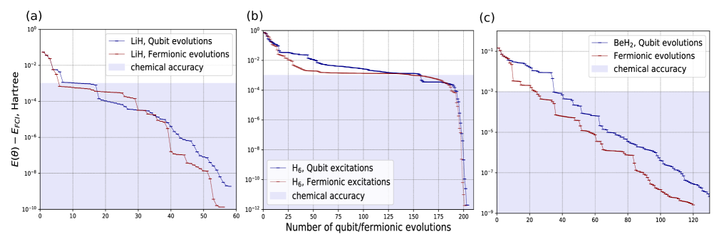
Figure 3 shows energy convergence plots, obtained with the two protocols as explained above, for the ground states of LiH (Fig. 3.a), H₆ (Fig. 3.b) and BeH₂ (Fig. 3.c) at bond distances of $r_{\text{Li-H}}=1.546{\textup{\AA}}$, $r_{\text{H-H}}=1.5{\textup{\AA}}$ and $r_{\text{Be-H}}=1.316{\textup{\AA}}$, respectively. All plots are terminated for $\epsilon=10^{-12}$ Hartree. The two protocols converge similarly, with the fermionic-ADAPT-VQE converging slightly faster for more than $\sim 50$ ansatz elements. This difference is most evident for the more strongly correlated H₆ (Fig. 3.b), where the fermionic-ADAPT-VQE requires up to $20\%$ fewer excitation evolutions than the QEB-ADAPT-VQE to achieve a given accuracy. These observations suggest that fermionic-excitation-based ansätze might be able to approximate strongly correlated states a bit better than qubit-excitation-based ansätze. To further investigate this observation, in Fig. 4 we include energy convergence plots, similar to those in Fig. 3, but for bond distances of $r_{\text{Li-H}}=3{\textup{\AA}}$ (Fig. 4.a), $r_{\text{H-H}}=3{\textup{\AA}}$ (Fig. 4.b) and $r_{\text{Be-H}}=3{\textup{\AA}}$ (Fig. 4.c). At larger bond distances the ground states of the LiH, and BeH₂ are more strongly correlated, so we expect to see larger difference in the convergence rates of the two protocols.

Figure 4: Comparison of qubit and fermionic excitation evolutions at large bond distances. The three subgifures present energy convergence plots for the ground states of: (a) LiH, (b) H₆ and (c) $\text{BeH}_{2}$, in the STO-3G orbital basis set, at bond distances of $r_{Li-H}=3\textup{\AA}$, $r_{H-H}=3\textup{\AA}$ and $r_{Be-H}=3\textup{\AA}$, respectively. The blue plots are obtained with the QEB-ADAPT-VQE for $n=1$ and step 5 not implemented. The red plots are obtained with the fermionic-ADAPT-VQE using an ansatz element pool of non-spin-complement fermionic excitation evolutions. The plots are terminated at $\epsilon=10^{-12}$ Hartree.

In Fig. 4a,c we see that for LiH and BeH₂, at $r_{\text{Li-H}}=3{\textup{\AA}}$ and $r_{\text{Be-H}}=3{\textup{\AA}}$, respectively, indeed there is a larger difference in the convergence rates of the two protocols, in favour of the fermionic-ADAPT-VQE. This is more evident for BeH₂ where the fermionic-ADAPT-VQE requires about $20\%$ fewer ansatz elements, on average, than the QEB-ADAPT-VQE, to achieve a given accuracy. These results further indicate that fermionic-excitation-based ansätze can approximate strongly correlated states better than qubit-excitation-based ansätze.

III.7 Energy dissociation curves

Figure 5 shows energy dissociation curves for LiH, H₆ and $\text{BeH}_{2}$, obtained with the QEB-ADAPT-VQE for $n=10$ and energy-reduction thresholds $\epsilon_{4}=10^{-4}$ Hartree, $\epsilon_{6}=10^{-6}$ Hartree and $\epsilon_{8}=10^{-8}$ Hartree. Dissociation curves obtained with the Hartree-Fock (HF) method, the full configuration interaction (FCI) method, and the VQE, using an untrotterized UCCSD ansatz (UCCSD-VQE) are also included for comparison. The UCCSD includes spin-conserving single and double fermionic evolutions only, for a fairer comparison to the QEB-ADAPT-VQE.

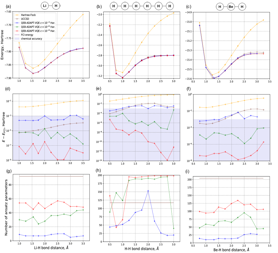
Figure 5: Energy dissociation curves for LiH, H₆ and $\text{BeH}_{2}$ molecules in the STO-3G orbital basis set. (a,b,c) Absolute energy as function of bond distance. (d,e,f) Energy error with respect to the exact FCI energy as function of bond distance. (g,h,i) Number of ansatz variational parameters required to reach the energy accuracies in (d,e,f). The QEB-ADAPT-VQE is performed for $n=10$ and step 5 implemented. The number of variational parameters for the UCCSD is $92$, $117$ and $204$ for LiH, H₆ and BeH₂, respectively. The number of variational parameters is also equivalent to the number of ansatz elements of each ansatz.

Figures 5a,b,c show the absolute values for the ground-state energy estimates. All methods except the HF, produce close energy estimates that cannot be clearly distinguished. In Figs. 5d,e,f the exact FCI energy is subtracted in order to differentiate better the different methods and their corresponding errors.

The UCCSD-VQE achieves chemical accuracy over all bond distances for LiH (Fig. 5d) and over bond distances close to equilibrium configuration for H₆(Fig. 5e) and BeH₂(Fig. 5f). However, the UCCSD-VQE fails to achieve chemical accuracy for bond distances away from equilibrium configuration for H₆ and BeH₂, where the ground states become more strongly correlated.

The QEB-ADAPT-VQE for $\epsilon_{4}$, similarly to the UCCSD-VQE, struggles to achieve chemical accuracy for strongly correlated ground states. However, for $\epsilon_{6}$ and $\epsilon_{8}$ the QEB-ADAPT-VQE achieves chemical accuracy over all investigated bond distances, for all three molecules. This indicates that the QEB-ADAPT-VQE can successfully construct ansätze to accurately approximate strongly correlated states.

However, the real strength of the QEB-ADAPT-VQE, similarly to other ADAPT-VQE protocols, is not just in constructing accurate ansätze, but in constructing accurate problem-tailored ansätze with few variational parameters, and corresponding shallow ansatz circuits. Figures 5g.h.i show plots of the number of variational parameters used by the ansatz of each method as function of bond distance. In the cases of LiH (Fig. 5g) and BeH₂ (Fig. 5i), the ansätze constructed by the QEB-ADAPT-VQE for $\epsilon_{6}$ and $\epsilon_{8}$ are not only more accurate than the UCCSD, but also have significantly fewer parameters. However, in the case of H₆ the QEB-ADAPT-VQE on average requires more parameters than the UCCSD. The reason for this is that H₆ is more strongly correlated than LiH and BeH₂, so even an optimally constructed ansatz would require more variational parameters than the UCCSD, to accurately approximate the ground state of H₆.

An interesting observation is the abrupt changes in the number of variational parameters used by the QEB-ADAPT-VQE for H₆ at bond distances of around $1\text{\AA}$ , $2\text{\AA}$, and $2.75\text{\AA}$. The reason for these changes are molecular structure transformations, where different eigenstates of H become lowest in energy (energy-level crossings).

III.8 Energy convergence

In this section we compare the QEB-ADAPT-VQE against the fermionic-ADAPT-VQE and the qubit-ADAPT-VQE using energy convergence plots (see Fig. 6). To ensure a fair comparison we choose the following settings for the three protocols: We perform the QEB-ADAPT-VQE for $n=1$, using an ansatz element pool of all unique single and double qubit excitation evolutions. The fermionic-ADAPT-VQE is performed as in Ref. Grimsley et al. (2019b), using a ansatz element pool of all unique single and double spin-complement fermionic excitation evolutions. For the qubit-ADAPT-VQE we use an ansatz element of all evolutions of $XY$-Pauli strings of length $2$ and $4$ that have an odd number of $Y$s. This pool consists of $O(N^{4})$ Pauli string evolutions that can be combined to obtain all qubit excitation evolutions in the ansatz element of the QEB-ADAPT-VQE (see Sec. “Ansatz elements”). Because of this the comparison between the QEB-ADAPT-VQE and qubit-ADAPT-VQE, in terms of ansatz-circuit efficiency, can be considered fair. We note that the authors of Ref. Tang et al. (2021) proved that the qubit-ADAPT-VQE actually can construct an ansatz that exactly recovers the FCI wavefunction, using a reduced ansatz element pool of only $2N_{MO}-2$ Pauli string evolutions. This reduced pool can decrease the number of quantum computer measurements required to evaluated the energy gradients at each iteration (see step 2 of the QEB-ADAPT-VQE) from $O(N_{MO}^{8})$ to $O(N_{MO}^{5})$. However, the reduced ansatz element pool will also result in a slower and less circuit-efficient ansatz construction, so using this reduced pool in the comparison with the QEB-ADAPT-VQE would not be fair.

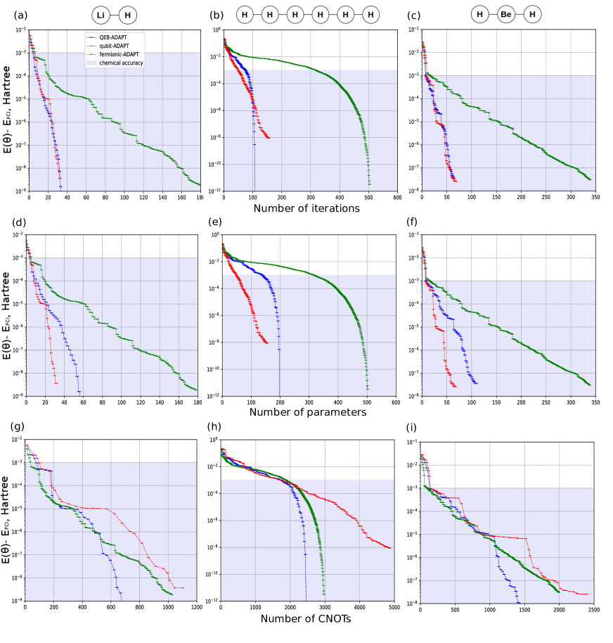
Figure 6: Comparison of the QEB-ADAPT-VQE, the fermionic-ADAPT-VQE and the qubit-ADAPT-VQE. The subfigures above present energy convergence plots for the ground states of LiH, H₆ and $\text{BeH}_{2}$, in the STO-3G orbital basis set, at bond distances $r_{\text{Li-H}}=1.546{\textup{\AA}}$, $r_{\text{H-H}}=1.5{\textup{\AA}}$ and $r_{\text{Be-H}}=1.316{\textup{\AA}}$. The plots compare the QEB-ADAPT-VQE (blue), the fermionic-ADAPT-VQE (red) and the qubit-ADAPT-VQE (green) protocols in terms of number of iterations (a,b,c), number of parameters (d,e,f) and number of $CNOT$s (g,h,i). The QEB-ADAPT-VQE is performed for $n=1$. All convergence plots are terminated for an energy-reduction threshold of $\epsilon=10^{-12}$ Hartree. The $CNOT$ counts in g,h,i are obtained assuming the use of the quantum circuits discussed in Sec. “Ansatz elements”.

We compare the three protocols in terms of three cost metrics, required to construct an ansatz to achieve a specific accuracy: (1) the number of iterations; (2) the number of variational parameters; and (3) the number of $CNOT$s. The number of iterations and the number of variational parameters (the number of iterations is the same as the number of variational parameters for the fermionic-ADAPT-VQE and the qubit-ADAPT-VQE, but not for the QEB-ADAPT-VQE) determine the total number of quantum computer measurements (see Supplementary Note 4). The $CNOT$ count of the ansatz circuit is approximately proportional to its depth. Hence, the $CNOT$ count can be used as a measure of the run time of the quantum subroutine of the VQE, which also reflects the error accumulated by the quantum hardware. Due to the limited coherence times of NISQ computers, the $CNOT$ count is considered as a primary cost metric.

Figure 6 shows energy convergence plots, obtained with the three ADAPT-VQE protocols, for LiH, H₆ and $\text{BeH}_{2}$ at bond distances of $r_{Li-H}=1.546{\textup{\AA}}$, $r_{H-H}=1.5{\textup{\AA}}$ and $r_{Be-H}=1.316{\textup{\AA}}$, respectively. All energy convergence plots are terminated at $\epsilon=10^{-12}$ Hartree.

In Figs. 6a,b,c we notice that the QEB-ADAPT-VQE and the fermionic-ADAPT-VQE perform similarly in terms of the number of iterations. This implies that the QEB-ADAPT-VQE and the fermionic-ADAPT-VQE use approximately the same number of qubit and fermionic excitation evolutions, respectively, when constructing their respective ansätze. This result is expected, because the two types of excitation evolutions perform similarly in constructing electronic wavefunction ansätze. Since qubit excitation evolutions are implemented by simpler circuits than fermionic excitation evolutions, the QEB-ADAPT-VQE systematically outperforms the fermionic-ADAPT-VQE in terms of $CNOT$ count in Figs. 6g,h,i.

While the QEB-ADAPT-VQE and the fermionic-ADAPT-VQE require similar numbers of iterations (Fig. 6a,b,c), the QEB-ADAPT-VQE requires up to twice as many variational parameters (Fig. 6d,e,f). This difference is due to the fact that the QEB-ADAPT-VQE assigns one parameter to each qubit excitation evolutions in its ansatz, whereas the fermionic-ADAPT-VQE assigns one parameter to a pair of spin-complement fermionic excitation evolutions.

Figures 6a,b,c,d show that the QEB-ADAPT-VQE converges faster, requiring systematically fewer iterations and variational parameters than the qubit-ADAPT-VQE. As suggested in Sec. “Ansatz elements”, this result is due to the fact that single and double qubit excitation evolutions correspond to combinations of $2$ and $8$ Pauli string exponentials.

In terms of CNOT count (Figs. 6 g,h,i), the qubit-ADAPT-VQE is more efficient than the QEB-ADAPT-VQE at low accuracies. However, for higher accuracies, and correspondingly larger ansätze, the QEB-VQE-ADAPT starts to systematically outperform the qubit-ADAPT-VQE in terms of $CNOT$-efficiency. This result can be attributed to the fact that qubit evolutions allow for the local circuit optimizations introduced in Ref. Yordanov et al. (2020), whereas Pauli string evolutions, albeit more variationally flexible, do not allow for any local circuit optimizations.

As a side point, it is interesting to note that when the fermionic-ADAPT-VQE is performed with a pool of independent single and double fermionic evolutions (Figs. 3 and 4) it is able to converge, albeit more slowly, to higher final accuracies than when it is performed with a pool of spin-complement pairs of single and double fermionic evolutions (Fig. 6). This is owing to the fact that the pool of independent fermionic excitation is more variationally flexible.

IV Discussion

In this work, we investigated the use of qubit excitations to construct electronic VQE ansätze. We demonstrated numerically that in general an ansatz of qubit excitation evolutions can approximate a molecular electronic wavefunction almost as accurately as an ansatz of fermionic excitation evolutions. However, fermionic-excitation-based ansätze were found to be slightly more accurate per number of excitation evolutions when approximating strongly correlated states. These results suggest that, on their own, the Pauli-$z$ strings, which measure the parity of the state and account for the anticommutation of the fermionic excitation operators, play little role in the variational flexibility of an electronic wavefunction ansatz. These results agree with previous findings in Refs. Xia and Kais (2020); Tang et al. (2021). Another advantage of fermionic excitation evolutions is that they can form spin-complement pairs of fermionic excitation evolutions. Such spin-complement pairs can then be used to enforce parity conservation and thus reduce the number of variational parameters of an ansatz by up to a factor of $2$. Nonetheless, fermionic excitation evolutions are implemented by circuits whose size, in terms of $CNOT$ count, scales linearly (logarithmically) in the Jordan-Wigner (Bravyi-Kitaev) encoding with the system size, as opposed to qubit excitation evolutions, which enjoy the quantum-computational benefit of being implemented by fixed-size circuits. Therefore, for NISQ devices, where the number of CNOTs is a primary cost factor, qubit excitation evolutions are more suitable for constructing electronic ansätze.

Motivated by the accuracy and circuit efficiency of qubit-excitations-based ansätze, we introduce the qubit-excitation based adaptive variational quantum eigensolver (QEB-ADAPT-VQE). The QEB-ADAPT-VQE simulates molecular electronic ground states with a problem-tailored ansatz, grown iteratively by appending single and double qubit excitation evolutions. We benchmarked the performance of the QEB-ADAPT-VQE with classical numerical simulations for LiH, H₆ and $\text{BeH}_{2}$. In particular, we compared the QEB-ADAPT-VQE to the original fermionic-ADAPT-VQE, and its more slowly converging, but more circuit-efficient cousin, the qubit-ADAPT-VQE. Compared to the fermionic-ADAPT-VQE, the QEB-ADAPT-VQE requires up to twice as many variational parameters. However, the QEB-ADAPT-VQE requires asymptotically fewer $CNOT$s, owing to its use of qubit excitation evolutions.

The simulations also showed that the qubit-ADAPT-VQE is more $CNOT$-efficient than the QEB-ADAPT-VQE in achieving low accuracies that correspond to small ansatz circuits. However, for higher accuracies and correspondingly larger ansatz circuits, the QEB-ADAPT-VQE systematically outperformed the qubit-ADAPT-VQE in terms of $CNOT$-efficiency. The primary reason for this is that qubit evolutions allow for local circuit optimizations, whilst the more rudimentary Pauli string evolutions, utilized by the qubit-ADAPT-VQE, do not. In practice, we are often just interest in reaching chemical accuracy. Therefore, one might question what is the usefulness of constructing more $CNOT$-efficient ansätze with the QEB-ADAPT-VQE for accuracies higher than chemical accuracy. Although the numerical results presented here are not sufficient to draw a general conclusion, they indicate that the $CNOT$-efficiency of the QEB-ADAPT-VQE becomes more evident for larger ansatz circuits. Therefore, for larger molecules, the QEB-ADAPT-VQE will likely be able to reach chemical accuracy using fewer $CNOT$s than the qubit-ADAPT-VQE. Our simulation results also demonstrated that in terms of convergence speed, the QEB-ADAPT-VQE requires fewer variational parameters, and correspondingly fewer ansatz-constructing iterations, than the qubit-ADAPT-VQE.

These results imply that the QEB-ADAPT-VQE is more circuit-efficient and converges faster than the qubit-ADAPT-VQE, which to our knowledge was the previously most circuit-efficient, scalable VQE protocol for molecular modelling. We do remark though, that in our comparison of the QEB-ADAPT-VQE and the qubit-ADAPT-VQE, we ignored the fact that the latter protocol can use a reduced ansatz element of $O(N_{MO})$ Pauli string evolutions, as shown in Ref. Tang et al. (2021). Using a reduced ansatz element pool would decrease the number of required quantum computer measurements, but will also result in a slower and less efficient ansatz construction. Moreover, the complexity of a single iteration of both the QEB-VQE-ADAPT and the qubit-ADAPT-VQE, might actually be dominated by running the VQE (see Supplementary Note 4). Therefore, reducing the size of the ansatz element pool might not affect the overall complexity of the protocol. We also note that, in theory, hardware-efficient ansätze and the ansätze of the IQCC protocol suggested in Refs. Ryabinkin et al. (2020); Lang et al. (2020) can be implement by shallower circuits than the ansätze constructed by the QEB-ADAPT-VQE. However, hardware-efficient ansätze and the IQCC are unlikely to be scalable for large systems: the optimization of hardware-efficient ansätze is likely to become intractable for large systems; and the IQCC requires evaluating a number of expectation values, exponential in the number of variational parameters.

As further work, three potential upgrades to the QEB-VQE-ADAPT can be considered. First, the ansatz element pool of the QEB-VQE-ADAPT can be expanded to include non-symmetry-preserving terms as suggested in Ref. Choquette et al. (2020). Potentially, this expanded pool could further improve the speed of convergence and boost the resilience to symmetry-breaking errors of the QEB-VQE-ADAPT. Second, methods from Ref. Sim et al. (2020) can be used to “prune”, from the already constructed ansatz, qubit excitation evolutions that have little contribution to the energy reduction. This could potentially optimize further the constructed ansatz. Third, the QEB-VQE-ADAPT functionality can be expanded to enable estimations of energies of low lying excited states. This will be the topic of another work (see Ref. Yordanov et al. (2021) for a preprint).

V Code availability

The code used to perform the numerical simulations presented in this paper is publicly available at https://github.com/JordanovSJ. Data generated during the study is available upon request from the authors (E-mail: yy387@cam.ac.uk or drma2@cam.ac.uk).

Appendix A Supplementary note 1

The expression for the single parameter energy gradient in equation (23) of the main text, can be derived as follows:

$$\frac{\partial}{\partial\theta_{p}}E^{(m-1)}(\theta_{p})=\frac{\partial}{\partial\theta_{p}}\langle\psi^{(m-1)}|\tilde{A_{p}}^{\dagger}(\theta_{p})H\tilde{A_{p}}(\theta_{p})|\psi^{(m-1)}\rangle=\frac{\partial}{\partial\theta_{p}}\langle\psi^{(m-1)}|e^{\theta_{p}\tilde{T_{p}}^{\dagger}}He^{\theta_{p}\tilde{T_{p}}}|\psi^{(m-1)}\rangle=$$

$$\langle\psi^{(m-1)}|e^{\theta_{p}\tilde{T_{p}}^{\dagger}}\tilde{T_{p}}^{\dagger}He^{\theta_{p}\tilde{T_{p}}}|\psi^{(m-1)}\rangle+\langle\psi^{(m-1)}|e^{\theta_{p}\tilde{T_{p}}^{\dagger}}H\tilde{T_{p}}e^{\theta_{p}\tilde{T_{p}}}|\psi^{(m-1)}\rangle=$$ (25)

$$\langle\psi^{(m-1)}|e^{\theta_{p}\tilde{T_{p}}^{\dagger}}[H,\tilde{T_{p}}]e^{\theta_{p}\tilde{T_{p}}}|\psi^{(m-1)}\rangle$$ (26)

In going from (25) to (26) we use that $\tilde{T_{p}}$ is skew-Hermitian, so that $\tilde{T_{p}}^{\dagger}=-\tilde{T_{p}}$. In the limit $\theta_{p}\rightarrow 0$ expression (26) becomes equivalent to the expression in equation (23) of the main text.

Appendix B Supplementary note 2

Here we outline the method used to calculate the trial statevectors $|\psi(\boldsymbol{\theta})\rangle$ in the classical numerical simulations used for the results in this paper. Calculating the trial statevectors, is the most time consuming part of the numerical simulations, and optimizing it is vital.

In this work, we are concerned with states of the form

$$|\psi(\boldsymbol{\theta})\rangle=U(\boldsymbol{\theta})|\psi_{0}\rangle=\prod_{i=N_{U}}^{1}e^{\theta_{i}S_{i}}|\psi_{0}\rangle,$$ (27)

where $N_{U}$ is the size (the number of ansatz elements) of the ansatz $U(\boldsymbol{\theta})$, $|\psi_{0}\rangle$ is the initial reference state, and $S_{i}$ is a skew-Hermitian operator, which in this paper corresponds to either a qubit excitation operator, a fermionic excitation operator, or a string of Pauli operators. Each of these three types of skew-Hermitian operators, also satisfies the relation

$$S_{i}^{3}=-S_{i}.$$ (28)

To calculate the $2^{N_{{}_{\mathrm{MO}}}}$-dimensional state-vector representing $|\psi(\boldsymbol{\theta})\rangle$, classically, we need to calculate the $N_{U}$ exponents $\{e^{\theta_{i}S_{i}}\}$ in equation (27), and then multiply them sequentially to $|\psi_{0}\rangle$. Each $S_{i}$ is represented by an $2^{N_{{}_{\mathrm{MO}}}}\times 2^{N_{{}_{\mathrm{MO}}}}$-dimensional matrix. Hence, the complexity of estimating each exponent $e^{\theta_{i}S_{i}}$, directly, is $O(2^{3N_{{}_{\mathrm{MO}}}})$. However, we can make use of relation (28) and write each exponent in equation (27) as

$$e^{\theta_{i}S_{i}}=\sum_{r=0}^{\infty}\frac{\theta_{i}^{r}S_{i}^{r}}{r!}=I+\sum_{r_{1}=0}^{\infty}\frac{(-1)^{r_{1}}\theta_{i}^{2r_{1}+1}}{(2r_{1}+1)!}S_{i}+\sum_{r_{2}=1}^{\infty}\frac{(-1)^{r_{2}}\theta_{i}^{2r_{2}}}{(2r_{2})!}S_{i}^{2}=I+\sin\theta S_{i}+(1-\cos\theta)S_{i}^{2}.$$ (29)

The operators $\{S_{i}\}$ are fixed throughout a simulation. Therefore, if we compute in advance and store the matrix representations of each $S_{i}$ and $S_{i}^{2}$, we can evaluate the expression in equation (29) by performing matrix addition only, which has a complexity of $O(2^{2N_{{}_{\mathrm{MO}}}})$. Hence, the calculation of $|\psi(\boldsymbol{\theta})\rangle$, requires $N_{U}$ matrix-to-vector multiplications and $N_{U}$ matrix additions, which gives a total complexity of $O(N_{U}2^{2N_{{}_{\mathrm{MO}}}})$.

The drawback of the method outlined above is that we need to store the matrices for all $S_{i}$ and $S_{i}^{2}$ operators. For example, the most memory demanding simulation in this work, running the qubit-ADAPT-VQE for $\text{BeH}_{2}$, required around $2$GB of RAM to store the matrices for all Pauli string operators, which define the ansatz element pool of the qubit-ADAPT-VQE, and their respective squares. However, in this case, a speed-up of nearly a factor of $20$ was achieved, in comparison to calculating $|\psi(\boldsymbol{\theta})\rangle$ with the general IBM’s Qiskit statevector simulator.

Appendix C Supplementary note 3

When using a gradient-descent minimizer, e.g. the BFGS, we have the option to supply a function that returns the gradient vector of the minimized function. If we are close to the global minimum, supplying a gradient vector function guarantees a faster optimization of the variational parameters. In the case of minimizing the Hamiltonian expectation value $E(\boldsymbol{\theta})=\langle\psi(\boldsymbol{\theta})|H|\psi(\boldsymbol{\theta})\rangle$, the $i^{\mathrm{th}}$ component of the energy gradient vector, $\boldsymbol{\nabla}E(\boldsymbol{\theta})$, is given by

$$\boldsymbol{\nabla}_{i}E(\boldsymbol{\theta})=\frac{\partial}{\partial\theta_{i}}\langle\psi(\boldsymbol{\theta})|H|\psi(\boldsymbol{\theta})\rangle=\frac{\partial}{\partial\theta_{i}}\langle\psi_{0}|U^{\dagger}(\boldsymbol{\theta})HU(\boldsymbol{\theta})|\psi_{0}\rangle=\frac{\partial}{\partial\theta_{i}}\langle\psi_{0}|\prod^{k_{1}=N_{U}}_{1}e^{\theta_{k_{1}}S^{\dagger}_{k_{1}}}H\prod_{k_{2}=N_{U}}^{1}e^{\theta_{k_{2}}S_{k_{2}}}|\psi_{0}\rangle=$$ (30)

$$\langle\psi(\boldsymbol{\theta})|H\prod_{k_{1}=N_{u}}^{i+1}e^{\theta_{k_{1}}S_{k_{1}}}S_{i}\prod_{k_{1}=i}^{1}e^{\theta_{k_{2}}S_{k_{2}}}|\psi_{0}\rangle+\langle\psi_{0}|\prod_{k_{1}=1}^{i}e^{\theta_{k_{1}}S^{\dagger}_{k_{1}}}S_{i}^{\dagger}\prod_{k_{1}=i+1}^{N_{U}}e^{\theta_{k_{2}}S^{\dagger}_{k_{2}}}|H|\psi(\boldsymbol{\theta})\rangle=2\langle\alpha_{i}(\boldsymbol{\theta})|S_{i}|\beta_{i}(\boldsymbol{\theta})\rangle,$$ (31)

where

$$|\beta_{i}(\boldsymbol{\theta})\rangle=\prod_{k=i}^{1}e^{\theta_{k}S_{k}}|\psi_{0}\rangle\ \ \text{and}$$ (32)

$$|\alpha_{i}(\boldsymbol{\theta})\rangle=\prod_{k=i+1}^{N_{u}}e^{\theta_{k}S_{k}^{\dagger}}H|\psi(\boldsymbol{\theta})\rangle,$$ (33)

and $N_{U}$ is the size (the number of ansatz elements) of the ansatz $U(\boldsymbol{\theta})$.

For the numerical simulations presented in this paper, the $N_{U}$ components of $\boldsymbol{\nabla}E(\boldsymbol{\theta})$ can be calculated with minimum number of matrix multiplications by updating $|\beta_{i}(\boldsymbol{\theta})\rangle$ and $|\alpha_{i}(\boldsymbol{\theta})\rangle$ in the following way:

1. For $i=N_{U}$, initiate

   $$|\alpha_{N_{U}}(\boldsymbol{\theta})\rangle=H|\psi(\boldsymbol{\theta})\rangle\ \ \text{and}$$ (34)

   $$|\beta_{N_{U}}(\boldsymbol{\theta})\rangle=|\psi(\boldsymbol{\theta})\rangle$$ (35)

2. For $1<i<N_{U}$, update

   $$|\alpha_{i-1}(\boldsymbol{\theta})\rangle=e^{\theta_{i}S_{i}^{\dagger}}|\alpha_{i}(\boldsymbol{\theta})\rangle\ \ \text{and}$$ (36)

   $$|\beta_{i-1}(\boldsymbol{\theta})\rangle=(e^{\theta_{i}S_{i}})^{-1}|\beta_{i}(\boldsymbol{\theta})\rangle=e^{\theta_{i}S_{i}^{\dagger}}|\beta_{i}(\boldsymbol{\theta})\rangle,$$ (37)

   where in equation (37), we use that $S_{i}$ is skew-Hermitian, so $S_{i}^{\dagger}=-S_{i}$.

Assuming that we have already computed and stored the matrices of the exponentials $\{e^{\theta_{i}S_{i}}\}$, when calculating $|\psi(\boldsymbol{\theta})\rangle$, to calculate each component of $\boldsymbol{\nabla}E(\boldsymbol{\theta})$ we need to perform $3$ matrix-to-vector multiplications. Thus, overall to calculate $\boldsymbol{\nabla}E(\boldsymbol{\theta})$ we need to perform $3N_{U}$ matrix-to-vector multiplications, resulting in a total cost of $O(3N_{U}2^{2N_{{}_{\mathrm{MO}}}})$ operations.

The cost of calculating $\boldsymbol{\nabla}E(\boldsymbol{\theta})$ is about $3$ times the cost of calculating $|\psi(\boldsymbol{\theta})\rangle$. However, we find that using the energy gradient vector in the optimization subroutine of the VQE, reduces the number of VQE iterations by at least an order of magnitude, which justifies the use of the gradient vector.

Appendix D Supplementary note 4

Here, we consider the computational complexity in terms of number of quantum computer measurements, and total run time. The computational complexity of the QEB-ADAPT-VQE is determined by steps 2 and 3.

Given that the electronic Hamiltonian, $H$, is represented by up to $O(N_{MO}^{4})$ Pauli strings (see equation (7) of the main text), calculating each gradient in step 2 would require $O(N_{MO}^{4})$ quantum computer measurements. Since $|\mathbb{P}(\tilde{A},N_{MO})|\propto N_{MO}^{4}$, the complexity of step 2, in terms of quantum computer measurements is $O(N_{MO}^{8})$. Step 2 is completely parallelizable so if multiple quantum computers are available, its time complexity can be arbitrarily reduced down to the time required to evaluate the expectation value of a single Pauli string term, which is proportional to the ansatz circuit depth, scaling as $O(m/N_{MO})$ (a $N_{MO}$-qubits circuit of $m$ qubit excitation evolutions), where $m$ is the iteration number of the QEB-ADAPT-VQE.

Using the BFGS minimizer, optimizing ansatz $U^{(m)}\big{(}\vec{\theta}^{(m)}\big{)}$, which has $O(m)$ variational parameters, would require $O(m^{2})$ VQE energy evaluations. Therefore, each VQE run in step 3 would require $O(m^{2}N_{MO}^{4})$ quantum computer measurement. Hence, the overall complexity of step 3 in terms of measurements would be $O(nm^{2}N_{MO}^{4})$. This complexity is a worst case estimate, assuming that at each iteration, all parameters $\vec{\theta}^{(m)}$ are initialized at zero. In fact, we initiate $\vec{\theta}^{(m)}$ as $\vec{\theta}^{(m-1)}\cup{0}$, so we will need fewer VQE energy evaluations to optimize the new ansatz, $U^{(m)}\big{(}\vec{\theta}^{(m)}\big{)}$. However, the complexity can also be higher if we use a direct search minimizer, like the Nelder-Mead, which is likely to be the case in practice, when noisy quantum hardware is used. Again, if multiple quantum devices are available, each of the $n$ VQE runs can be executed in parallel. Hence, the time complexity would be lower bounded by the run-time of a single VQE run, $O(m^{3}/N_{MO})$ (the ansatz circuit depth is $O(m/N_{MO})$ and we need to perform $O(m^{2})$ VQE energy evaluations).

Overall, the QEB-ADAPT-VQE would require $O\big{(}N_{U}(N_{MO}^{8}+nN_{U}^{2}N_{MO}^{4})\big{)}$ quantum computer measurements, and its run-time complexity would be lower bounded by $O(N_{U}^{4}/N_{MO})$. The size of the ansatz, $N_{U}$, depends on the desired accuracy, and also is problem specific. Therefore, it is difficult to predict how it would scale with $N_{MO}$. For strongly correlated states, achieving chemical accuracy might require an ansatz that consist of as many as $O(N_{MO}^{4})$ qubit excitation evolutions. However, for weakly correlated states, the scaling of $N_{U}$ with $N_{MO}$ is likely to be lower. Assuming the worst case scenario, the time complexity of the QEB-ADAPT-VQE will be lower-bounded by $O(N_{MO}^{15})$ and it will require $O(nN_{MO}^{16})$ quantum computer measurements. For comparison, the UCCSD-VQE has a time complexity of $O(N_{MO}^{11})$, assuming maximum parallelization, and requires $O(N_{MO}^{12})$ quantum computer measurements.

Appendix E Supplementary note 5

Here, we investigate the performance of the QEB-ADAPT-VQE for different values of $n$, the number of qubit excitation evolutions considered in step 3 of the QEB-ADAPT-VQE. As we increase $n$, we increase the chance to pick at each iteration the qubit excitation evolution that, added to the ansatz, achieves largest energy reduction. Following this greedy strategy is no guarantee for an optimal ansatz, since qubit evolutions do not commute in general. Nevertheless, we do expect, on average, to construct a more circuit-efficient ansatz by increasing $n$ up to some saturation value.

To test this presumption we perform classical numerical simulations to obtain energy convergence plots for the ground states of LiH, H₆ and BeH₂ in the STO-3G basis. The simulations for the three molecules are performed for bond distances $r_{Li-H}=3\text{\AA}$, $r_{H-H}=3\text{\AA}$ and $r_{Be-H}=3\text{\AA}$, away from equilibrium configurations, where correlation effects are stronger, and the effect of increasing $n$ should be more evident. The simulation results are presented in Supplementary figure 7.

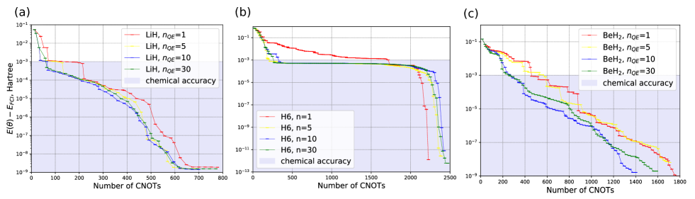
Figure 7: Performance of the QEB-ADAPT-VQE for different values of the protocol parameter $n$. The subfigures above present energy convergence plots obtained with the QEB-ADAPT-VQE with different values of $n$ for the ground states of LiH (a), H₆ (b) and BeH₂ (c) in the SO-3G basis, at bond distances of $r_{Li-H}=3\text{\AA}$, $r_{H-H}=3\text{\AA}$ and $r_{Be-H}=3\text{\AA}$. The plots are terminated at $\epsilon=10^{-12}$ Hartree.

The table below summarizes the average (over number of qubit excitation evolutions) $CNOT$ count reductions, with respect to $n=1$, for each molecule and different value of $n$:

	$n=5$	$n=10$	$n=30$
LiH	$16\%$	$20\%$	$16\%$
BeH2	$3\%$	$26\%$	$22\%$
H6	$15\%$	$12\%$	$13\%$

Table 1: Average (over number of qubit excitation evolutions) $CNOT$ count reduction for QEB-ADAPT-VQE($n_{qe}>1$) as compared to QEB-ADAPT-VQE($n_{qe}=1$).

For LiH (Supplementary figure 7.a), the QEB-ADAPT-VQE clearly constructs ansatz circuits with fewer $CNOT$s as $n$ is increased above $1$. For BeH₂ (Supplementary figure 7.c), a significant $CNOT$ count reduction is obtained for $n=10$ and $n=30$, but not for $n=5$. For H₆ (Supplementary figure 7.b), the average $CNOT$ reduction is about the same for $n=5$, $n=10$ and $n=30$, but strangely the ansatz constructed by the QEB-ADAPT-VQE for $n=1$ is the most $CNOT$-efficient for accuracies higher than $10^{-4}$ Hartree. Also, for all three molecules we observe no further $CNOT$ reduction for $n=30$ as compared to $n=10$. Actually for $n=30$ the $CNOT$ reduction is a bit lower. As noted above these inconsistencies can be explained by the fact that the greedy strategy to obtain the lowest estimate for $E(\vec{\theta})$ at each iteration is no guarantee for constructing an optimal ansatz, because qubit excitation evolutions do not commute.

Nonetheless, there is a clear advantage in terms of $CNOT$ count, in performing step 3 of the QEB-ADAPT-VQE for $n>1$. Despite the associated overhead in the number of quantum computer measurements with increasing $n$, this is justified as long as the bottleneck of NISQ computers is the quantum gate fidelity. Furthermore, we can expect the $CNOT$ count reduction for $n>1$ to increase for larger molecules, because the QEB-ADAPT-VQE will have to consider a larger ansatz element pool.

References

- Benioff (1980) P. Benioff, Journal of statistical physics 22, 563 (1980).
- Feynman (1999) R. P. Feynman, Int. J. Theor. Phys 21 (1999).
- Preskill (2018) J. Preskill, Quantum 2, 79 (2018).
- Arute et al. (2019) F. Arute, K. Arya, R. Babbush, D. Bacon, J. C. Bardin, R. Barends, R. Biswas, S. Boixo, F. G. Brandao, D. A. Buell, et al., Nature 574, 505 (2019).
- Elfving et al. (2020) V. E. Elfving, B. W. Broer, M. Webber, J. Gavartin, M. D. Halls, K. P. Lorton, and A. Bochevarov, (2020), arXiv:2009.12472 .
- McArdle et al. (2020) S. McArdle, S. Endo, A. Aspuru-Guzik, S. C. Benjamin, and X. Yuan, Rev. Mod. Phys. 92, 015003 (2020).
- McClean et al. (2016) J. R. McClean, J. Romero, R. Babbush, and A. Aspuru-Guzik, New Journal of Physics 18, 023023 (2016).
- Cerezo et al. (2020a) M. Cerezo, A. Arrasmith, R. Babbush, S. C. Benjamin, S. Endo, K. Fujii, J. R. McClean, K. Mitarai, X. Yuan, L. Cincio, et al., arXiv preprint arXiv:2012.09265 (2020a).
- O’Malley et al. (2016) P. J. J. O’Malley, R. Babbush, I. D. Kivlichan, J. Romero, J. R. McClean, R. Barends, J. Kelly, P. Roushan, A. Tranter, N. Ding, B. Campbell, Y. Chen, Z. Chen, B. Chiaro, A. Dunsworth, A. G. Fowler, E. Jeffrey, E. Lucero, A. Megrant, J. Y. Mutus, M. Neeley, C. Neill, C. Quintana, D. Sank, A. Vainsencher, J. Wenner, T. C. White, P. V. Coveney, P. J. Love, H. Neven, A. Aspuru-Guzik, and J. M. Martinis, Phys. Rev. X 6, 031007 (2016).
- Wang et al. (2019) D. Wang, O. Higgott, and S. Brierley, Phys. Rev. Lett. 122, 140504 (2019).
- Arute et al. (2020) F. Arute, K. Arya, R. Babbush, D. Bacon, J. C. Bardin, R. Barends, S. Boixo, M. Broughton, B. B. Buckley, D. A. Buell, et al., arXiv preprint arXiv:2004.04174 (2020), 10.1126/science.abb9811.
- Gonthier et al. (2020) J. F. Gonthier, M. D. Radin, C. Buda, E. J. Doskocil, C. M. Abuan, and J. Romero, arXiv preprint arXiv:2012.04001 (2020).
- Nielsen and Chuang (2002) M. A. Nielsen and I. Chuang, “Quantum computation and quantum information,” (2002).
- Dorner et al. (2009) U. Dorner, R. Demkowicz-Dobrzanski, B. J. Smith, J. S. Lundeen, W. Wasilewski, K. Banaszek, and I. A. Walmsley, Phys. Rev. Lett. 102, 040403 (2009).
- Helgaker et al. (2014) T. Helgaker, P. Jorgensen, and J. Olsen, Molecular electronic-structure theory (John Wiley & Sons, 2014).
- Peruzzo et al. (2014) A. Peruzzo, J. McClean, P. Shadbolt, M.-H. Yung, X.-Q. Zhou, P. J. Love, A. Aspuru-Guzik, and J. L. O’brien, Nature communications 5, 4213 (2014).
- Hempel et al. (2018) C. Hempel, C. Maier, J. Romero, J. McClean, T. Monz, H. Shen, P. Jurcevic, B. P. Lanyon, P. Love, R. Babbush, A. Aspuru-Guzik, R. Blatt, and C. F. Roos, Phys. Rev. X 8, 031022 (2018).
- Romero et al. (2018) J. Romero, R. Babbush, J. R. McClean, C. Hempel, P. J. Love, and A. Aspuru-Guzik, Quantum Science and Technology 4, 014008 (2018).
- Harsha et al. (2018) G. Harsha, T. Shiozaki, and G. E. Scuseria, The Journal of chemical physics 148, 044107 (2018).
- Bauman et al. (2021) N. Bauman, J. Chládek, L. Veis, J. Pittner, and K. Kowalski, Quantum Science and Technology (2021).
- Dallaire-Demers et al. (2019) P.-L. Dallaire-Demers, J. Romero, L. Veis, S. Sim, and A. Aspuru-Guzik, Quantum Science and Technology 4, 045005 (2019).
- Sokolov et al. (2020) I. O. Sokolov, P. K. Barkoutsos, P. J. Ollitrault, D. Greenberg, J. Rice, M. Pistoia, and I. Tavernelli, The Journal of Chemical Physics 152, 124107 (2020).
- Nam et al. (2020) Y. Nam, J.-S. Chen, N. C. Pisenti, K. Wright, C. Delaney, D. Maslov, K. R. Brown, S. Allen, J. M. Amini, J. Apisdorf, et al., npj Quantum Information 6, 1 (2020).
- Lee et al. (2018) J. Lee, W. J. Huggins, M. Head-Gordon, and K. B. Whaley, Journal of chemical theory and computation 15, 311 (2018).
- Grimsley et al. (2019a) H. R. Grimsley, D. Claudino, S. E. Economou, E. Barnes, and N. J. Mayhall, Journal of Chemical Theory and Computation (2019a), https://doi.org/10.1021/acs.jctc.9b01083.
- Kandala et al. (2017) A. Kandala, A. Mezzacapo, K. Temme, M. Takita, M. Brink, J. M. Chow, and J. M. Gambetta, Nature 549, 242 (2017).
- Kandala et al. (2018) A. Kandala, K. Temme, A. D. Corcoles, A. Mezzacapo, J. M. Chow, and J. M. Gambetta, arXiv preprint arXiv:1805.04492 (2018), 10.1038/s41586-019-1040-7.
- Ganzhorn et al. (2019) M. Ganzhorn, D. J. Egger, P. Barkoutsos, P. Ollitrault, G. Salis, N. Moll, M. Roth, A. Fuhrer, P. Mueller, S. Woerner, et al., Physical Review Applied 11, 044092 (2019).
- Barkoutsos et al. (2018) P. K. Barkoutsos, J. F. Gonthier, I. Sokolov, N. Moll, G. Salis, A. Fuhrer, M. Ganzhorn, D. J. Egger, M. Troyer, A. Mezzacapo, S. Filipp, and I. Tavernelli, Phys. Rev. A 98, 022322 (2018).
- Gard et al. (2020) B. T. Gard, L. Zhu, G. S. Barron, N. J. Mayhall, S. E. Economou, and E. Barnes, npj Quantum Information 6, 1 (2020).
- Bittel and Kliesch (2021) L. Bittel and M. Kliesch, arXiv preprint arXiv:2101.07267 (2021).
- McClean et al. (2018) J. R. McClean, S. Boixo, V. N. Smelyanskiy, R. Babbush, and H. Neven, Nature communications 9, 1 (2018).
- Wang et al. (2020) S. Wang, E. Fontana, M. Cerezo, K. Sharma, A. Sone, L. Cincio, and P. J. Coles, arXiv preprint arXiv:2007.14384 (2020).
- Cerezo et al. (2020b) M. Cerezo, A. Sone, T. Volkoff, L. Cincio, and P. J. Coles, arXiv preprint arXiv:2001.00550 (2020b).
- Abbas et al. (2020) A. Abbas, D. Sutter, C. Zoufal, A. Lucchi, A. Figalli, and S. Woerner, arXiv preprint arXiv:2011.00027 (2020).
- Grimsley et al. (2019b) H. R. Grimsley, S. E. Economou, E. Barnes, and N. J. Mayhall, Nature communications 10, 1 (2019b).
- Tang et al. (2021) H. L. Tang, V. Shkolnikov, G. S. Barron, H. R. Grimsley, N. J. Mayhall, E. Barnes, and S. E. Economou, PRX Quantum 2, 020310 (2021).
- Rattew et al. (2019) A. G. Rattew, S. Hu, M. Pistoia, R. Chen, and S. Wood, arXiv preprint arXiv:1910.09694 (2019).
- Ryabinkin et al. (2020) I. G. Ryabinkin, R. A. Lang, S. N. Genin, and A. F. Izmaylov, Journal of Chemical Theory and Computation 16, 1055 (2020).
- Lang et al. (2020) R. A. Lang, I. G. Ryabinkin, and A. F. Izmaylov, arXiv preprint arXiv:2002.05701 (2020).
- Sim et al. (2020) S. Sim, J. Romero, J. F. Gonthier, and A. A. Kunitsa, arXiv preprint arXiv:2010.00629 (2020).
- Daniel Claudino and Humble (2020) A. J. M. Daniel Claudino, Jerimiah Wright and T. S. Humble, arXiv preprint arXiv:2011.01279 (2020).
- Matsuo (2020) A. Matsuo, arXiv preprint arXiv:2006.05643 (2020).
- Liu et al. (2020) J. Liu, Z. Li, and J. Yang, arXiv preprint arXiv:2012.07047 (2020).
- Xia and Kais (2020) R. Xia and S. Kais, Quantum Science and Technology (2020), https://doi.org/10.1088/2058-9565/abbc74.
- Wu and Lidar (2002) L.-A. Wu and D. Lidar, Journal of Mathematical Physics 43, 4506 (2002).
- Yordanov et al. (2020) Y. S. Yordanov, D. R. M. Arvidsson-Shukur, and C. H. W. Barnes, Phys. Rev. A 102, 062612 (2020).
- Wigner and Jordan (1928) E. Wigner and P. Jordan, Z. Phys 47, 631 (1928).
- Bravyi and Kitaev (2002) S. B. Bravyi and A. Y. Kitaev, Annals of Physics 298, 210 (2002).
- Mazziotti (2020) D. A. Mazziotti, Phys. Rev. A 102, 030802 (2020).
- Nooijen (2000) M. Nooijen, Phys. Rev. Lett. 84, 2108 (2000).
- Whitfield et al. (2011) J. D. Whitfield, J. Biamonte, and A. Aspuru-Guzik, Molecular Physics 109, 735 (2011).
- Helgaker et al. (2012) T. Helgaker, S. Coriani, P. Jorgensen, K. Kristensen, J. Olsen, and K. Ruud, Chemical reviews 112, 543 (2012).
- McClean et al. (2020) J. McClean, N. Rubin, K. Sung, I. D. Kivlichan, X. Bonet-Monroig, Y. Cao, C. Dai, E. S. Fried, C. Gidney, B. Gimby, et al., Quantum Science and Technology (2020), 10.1088/2058-9565/ab8ebc.
- Ditchfield et al. (1971) R. Ditchfield, W. J. Hehre, and J. A. Pople, The Journal of Chemical Physics 54, 724 (1971).
- Hehre et al. (1969) W. J. Hehre, R. F. Stewart, and J. A. Pople, The Journal of Chemical Physics 51, 2657 (1969).
- Fletcher (2013) R. Fletcher, Practical methods of optimization (John Wiley & Sons, 2013).
- Virtanen et al. (2020) P. Virtanen, R. Gommers, T. E. Oliphant, M. Haberland, T. Reddy, D. Cournapeau, E. Burovski, P. Peterson, W. Weckesser, J. Bright, et al., Nature methods 17, 261 (2020).
- Podewitz et al. (2011) M. Podewitz, M. T. Stiebritz, and M. Reiher, Faraday discussions 148, 119 (2011).
- Lavrijsen et al. (2020) W. Lavrijsen, A. Tudor, J. Müller, C. Iancu, and W. de Jong, arXiv preprint arXiv:2004.03004 (2020).
- Nelder and Mead (1965) J. A. Nelder and R. Mead, The Computer Journal 7, 308 (1965), https://academic.oup.com/comjnl/article-pdf/7/4/308/1013182/7-4-308.pdf .
- Kokail et al. (2019) C. Kokail, C. Maier, R. van Bijnen, T. Brydges, M. K. Joshi, P. Jurcevic, C. A. Muschik, P. Silvi, R. Blatt, C. F. Roos, et al., Nature 569, 355 (2019).
- Barron et al. (2020) G. S. Barron, B. T. Gard, O. J. Altman, N. J. Mayhall, E. Barnes, and S. E. Economou, arXiv preprint arXiv:2003.00171 (2020).
- Choquette et al. (2020) A. Choquette, A. Di Paolo, P. K. Barkoutsos, D. Sénéchal, I. Tavernelli, and A. Blais, arXiv preprint arXiv:2008.01098 (2020).
- Yordanov et al. (2021) Y. S. Yordanov, C. H. Barnes, and D. R. Arvidsson-Shukur, arXiv preprint arXiv:2106.06296 (2021).