Gas compression and stellar feedback in the tidally interacting and ram-pressure stripped Virgo spiral galaxy NGC 4654

Due to an environment that promotes gravitational interactions and ram pressure stripping, galaxies within clusters are particularly likely to present unusual interstellar medium (ISM) properties. NGC 4654 is a Virgo cluster galaxy seen almost face-on, which undergoes nearly edge-on gas ram pressure stripping and a fly-by gravitational interaction with another massive galaxy, NGC 4639. NGC 4654 shows a strongly compressed gas region near the outer edge of the optical disk, with $\rm{H\textsc{i}}$ surface densities ($\rm{high\ H\textsc{i}\ surface\ density\ region}$) significantly exceeding the canonical value of 10-15 $\rm{M_{\odot}pc^{-2}}$. New IRAM 30m HERA CO(2-1) data of NGC 4654 are used to study the physical conditions of the ISM and its ability to form stars in the region where gas compression occurs. The CO-to-H₂ conversion factor was estimated by (i) simultaneously solving for the conversion factor and the dust-to-gas ratio by assuming that the latter is approximately constant on giant molecular cloud scales and (ii) by assuming that the dust-to-gas ratio is proportional to the metallicity. The CO-to-H₂ conversion factor was found to be one to two times the Galactic value. Based on the comparison with a region of similar properties in NGC 4501, we favor the higher value. We observe a significant decrease in the ratio between the molecular fraction and the total ISM pressure in the $\rm{high\ H\textsc{i}\ surface\ density\ region}$. The gas in this region is self-gravitating, with a Toomre parameter below the critical value of $Q=1$. However, the star-formation efficiency ($\rm SFE_{H_{2}}=\Sigma_{SFR}/\Sigma_{H_{2}}$) is 1.5 to 2 times higher, depending on the assumed conversion factor, in the $\rm{high\ H\textsc{i}\ surface\ density\ region}$ than in the rest of the disk. Analytical models were used to reproduce radial profiles of the SFR and the atomic and molecular surface densities to better understand which physical properties are mandatory to maintain such $\rm{high\ H\textsc{i}\ surface\ density\ region}$s. We conclude that a Toomre parameter of $\rm Q\sim 0.8$ combined with an increase in the velocity dispersion of $\Delta v_{\rm disp}\sim 5\ \rm{km\leavevmode\nobreak\ s^{-1}}$ are necessary conditions to simultaneously reproduce the gas surface densities and the SFR. A dynamical model that takes into account both gravitational interactions and ram pressure stripping was used to reproduce the gas distribution of NGC 4654. While the ISM properties are well reproduced in the whole disk, we find that the model SFR is significantly underestimated in the $\rm{high\ H\textsc{i}\ surface\ density\ region}$ due to the absence of gas cooling and stellar feedback. The comparison between the velocity dispersion given by the moment 2 map and the intrinsic 3D velocity dispersion from the model were used to discriminate between regions of broader linewidths caused by a real increase in the velocity dispersion and those caused by an unresolved velocity gradient only. We found that the 5 km s^-1 increase in the intrinsic velocity dispersion predicted by the model is compatible with the observed velocity dispersion measured in the $\rm{high\ H\textsc{i}\ surface\ density\ region}$. During a period of gas compression through external interactions, the gas surface density is enhanced, leading to an increased SFR and stellar feedback. Our observations and subsequent modeling suggest that, under the influence of stellar feedback, the gas density increases only moderately (by less than a factor of two). The stellar feedback acts as a regulator of star-formation, significantly increasing the turbulent velocity within the region.

1 Introduction

To understand how galaxies form stars from gas, it is essential to study disturbed disk galaxies. This is because it is possible to observe the influence of the perturbations on the interstellar medium (ISM) and its ability to form stars in these systems.

Galaxy clusters represent ideal laboratories for studying perturbations due to environmental interactions. Proximity between individual galaxies promotes gravitational interactions (slow galaxy-galaxy interactions or harassment) that affect both the stellar and dense gas distribution on larges scales. Moreover, the hydrodynamical interaction created by the motion of a galaxy through the hot and tenuous gas that constitutes the intracluster medium (ICM) also strongly affects the distribution of the interstellar medium (ISM). This effect - known as ram pressure stripping - depends on the ICM density and the velocity of the galaxy with respect to the cluster mean. Both quantities increase with a decreasing distance to the cluster center.

The main ingredient required for star-formation is dense molecular gas. Within spiral galaxies, a strong correlation has been identified between the molecular gas ($\rm{H_{2}}$) and the star-formation rate (SFR) (e.g, Kennicutt 1998, Bigiel et al. 2008, Kennicutt & Evans 2012, Bolatto et al. 2017). Therefore, one of the major quantities that has to be investigated is the star-formation efficiency with respect to the molecular gas, $\rm{SFE_{\rm{H_{2}}}}$. Past studies have shown that variations in the $\rm{SFE_{\rm{H_{2}}}}$ are wider between galaxies than within the same galactic disk (e.g, Leroy et al. 2008, Bigiel et al. 2008, Genzel et al. 2010, Schruba et al. 2011, Saintonge et al. 2017, Tacconi et al. 2018). The molecular ISM usually presents a constant depletion time of $t_{\rm{dep}}^{\rm{H_{2}}}$ $\rm\sim 2.35\ Gyr$ with a 1$\sigma$ scatter of 0.24dex (Bigiel et al. 2011). Only few extreme cases of interacting galaxies where the star-formation efficiency is significantly different have been found. This is the case for NGC 4438, which undergoes a tidal interaction and ram pressure stripping with $t_{\rm{dep}}^{\rm{H_{2}}}$ $\rm\sim 6\ Gyr$ (Vollmer et al. 2009, Vollmer et al. 2012b), as well as the Taffy system, a head-on collision between two massive spiral galaxies with $t_{\rm{dep}}^{\rm{H_{2}}}$ $\rm\sim 6\ Gyr$ (Vollmer et al. 2012a). Wong & Blitz (2002) highlighted a second correlation that describes the division of the molecular and the atomic phases within the ISM. The molecular fraction $R_{\rm{mol}}$ $\equiv$ $\rm{\Sigma_{\rm{H_{2}}}}$/$\rm{\Sigma_{\rm{HI}}}$ is approximately proportional to the total ISM pressure, $P_{\rm tot}$ (see Eq. 15). The natural question that arises from this observation is whether or not we can find galaxies among the cases of disturbed disk galaxies, especially those affected by ram pressure stripping, where these relations do not hold.

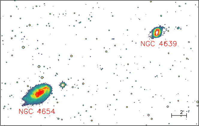
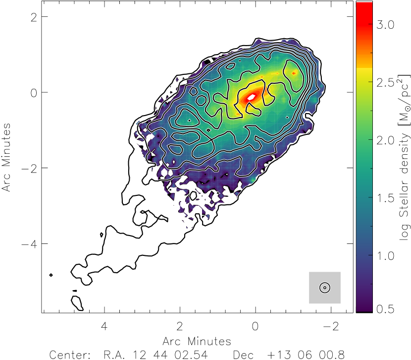
Figure 1: Environment and interstellar medium distribution of NGC 4654. Top panel: NGC 4654 and its companion NGC 4639 (SDSS9 extracted via Aladin v10 (Nebot Gomez-Moran et al. 2020)). Bottom panel: Hi surface density (contours) on the stellar surface density based on 3.6 $\rm{\mu}m$ SPITZER data (color). Contour levels are 1, 5, 10, 15, 20, and 30 $\rm{M_{\odot}pc^{-2}}$. The resolution is 16”.

Using the VIVA survey (VLA Imaging of Virgo galaxies in Atomic gas), Chung et al. (2007) revealed the presence of seven galaxies within the Virgo cluster with truncated $\rm{H\textsc{i}}$ disks and an extended $\rm{H\textsc{i}}$ gas tail on the opposite side. Among this sample, one galaxy in particular attracts our attention, NGC 4654. The $\rm{H\textsc{i}}$ disk of NGC 4654 is sharply truncated in the northwestern side of the disk and presents an unusually dense region of atomic hydrogen surface density (about 25 $\rm{M_{\odot}pc^{-2}}$ including Helium) at the edge of the optical disk (Fig. 1.). Such high surface densities are exceptional and have only been observed in very rare cases (e.g, in the interacting Eyelid galaxy, Elmegreen et al. 2016). In addition to being affected by ram pressure stripping, NGC 4654 underwent a gravitational interaction with another Virgo galaxy, NGC 4639, about 500 millions years ago (Vollmer 2003). NGC 4654 presents an asymmetric stellar distribution with a dense stellar arm toward the northwest (Fig. 1). A strongly enhanced $\rm{H\alpha}$ emission is also observed in the region of the highest atomic gas surface density (Fig. 2). The gravitational interaction and ram pressure stripping gave rise to asymmetric ridges of polarized radio continuum emission whereas the sudden ridge is most probably due to shear motions induced by the gravitational interaction and the western ridge is caused by ram pressure compression (Soida et al. 2006).

Table 1: NGC 4654 general properties

Morphological type	SAB(rs)cd
Optical diameter	5.17’ $\times$ 1.41’
Distance	17 Mpc
$\alpha$(J2000)	12h 43m 56.6s
$\delta$(J2000)	13$\degree$ 07’ 36”
Inclination angle	51$\degree$
Systemic velocity	1060 $\rm km\ s^{-1}$
Rotational velocity	170 $\rm km\ s^{-1}$
Total SFR	1.84 M⊙/yr
$\rm{H\textsc{i}}$ mass	3.4 $\times$ 109 M⊙
H2 mass	2.3 $\times$ 109 M⊙
Stellar mass	2.8 $\times$ 1010 M⊙

Chung & Kim (2014) conducted a study on NGC 4654 by combining the $\rm{H\textsc{i}}$ VIVA data with the extragalactic CO CARMA Survey Toward Infrared- bright Nearby Galaxies (STING, Rahman et al. 2011). They showed that the star-formation efficiency with respect to the molecular gas ($\rm SFE_{H_{2}}$) reaches unusually high values in the northwestern, high atomic gas surface density region. At the same time, they found that the R_mol/P_tot ratio is unusually low in this same region. As the $\rm{SFE_{\rm{H_{2}}}}$ and $R_{\rm{mol}}/P_{\rm{tot}}$ both depend on the surface density of the molecular gas, it is essential to determine the CO-to-$\rm{H_{2}}$ conversion factor as precisely as possible.

The purpose of this paper is to investigate the influence of gas compression and stellar feedback on the gas distribution and SFR within spiral galaxies through the study of NGC 4654 and its overdense northwestern region. We refer to the high atomic gas surface density region as ”Hi$\Sigma_{\rm HI}$” for the remainder of the paper. This article is organized in the following way. In Sect. 2 and Sect. 3, the new CO(2-1) IRAM 30m data are presented, with ancillary data in introduced in Sect. 4. The CO-to-H₂ conversion factor is estimated using the HERSCHEL 250$\rm\mu m$ data and direct metallicity measurements from Skillman et al. (1996) in Sect. 5. In Sect. 6, we use this conversion factor to compute molecular and the total gas maps of NGC 4654, and use the resulting maps to investigate the relation between molecular fraction and total mid-plane pressure of the gas (Sect. 7), the star-formation efficiency (Sect. 8), and the Toomre stability criterion (Sect. 9). An analytical model is used in Sect. 10.1 to reproduce the observed radial profiles. In Sect. 10.2, a dynamical model is used to reproduce the available observations. All the results are discussed in Sect. 11. We give our conclusions in Sect. 12. The general physical properties used for NGC 4654 in this study are presented in Table 1.

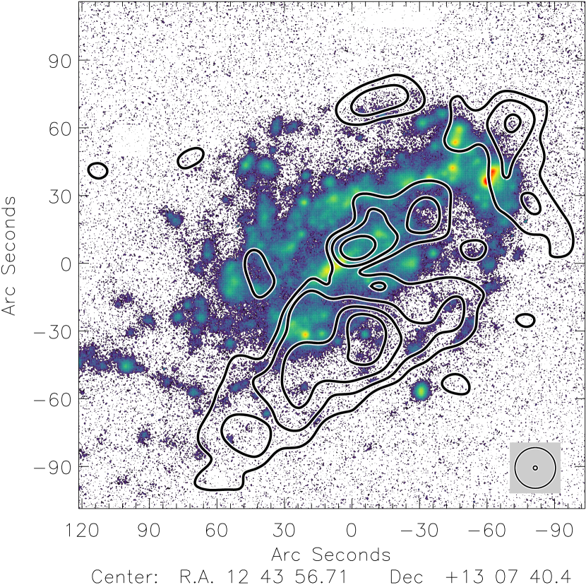
Figure 2: NGC 4654: 6cm polarized radio continuum emission (contours) on the GOLDMINE H$\alpha$ emission map in color levels (Gavazzi et al. 2003). The spatial resolutions are 18” and 1.8”.

2 Observations

NGC 4654 CO(2-1) data were observed by François Nehlig with the IRAM 30m single-dish telescope at Pico Veleta, Spain. OTF maps have been done to cover the entire galaxy using EMIR instrument in four different positions with a scanning speed of 5”/s, using FTS backends. The velocity window goes from 770 $\rm km\ s^{-1}$ to 1410 $\rm km\ s^{-1}$ with spectral resolution channel of 10.4 $\rm km\ s^{-1}$. We reached an average rms noise of 7 mK after a total of 25 hours of observation. We obtained a data cube with a spatial resolution of 12” using CLASS GILDAS xy_map routine. The pixel size is 3”. Compared to the interferometric data CARMA STING used by Chung & Kim (2014) our data are four times deeper and are sensitive to extended large-scale emission.

We produced CO moment maps using the VIVA $\rm{H\textsc{i}}$ data cube assuming that the CO line is located within the $\rm{H\textsc{i}}$ line profile (see Vollmer et al. 2012a). To do so, we resampled the channels of the $\rm{H\textsc{i}}$ data cube to fit the CO data cube. A first 3D binary mask was produced by clipping the $\rm{H\textsc{i}}$ data cube at the 4$\sigma$ level. For the CO data cube, we calculated the rms noise level for each spectrum at velocities devoid of an $\rm{H\textsc{i}}$ signal and subtracted a constant baseline. A second 3D binary mask was produced based on the CO data cube. If the maximum intensity of a spectrum exceeded 5 times the rms, we fit a Gaussian profile to the CO spectrum and fixed the mask limit to $\pm$3.2$\sigma$. The $\rm{H\textsc{i}}$ and CO 3D binary masks were added, applied to the CO data cube, and moment 0, 1, and 2 maps were created.

3 Results

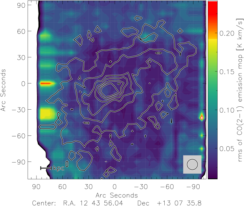
Figure 31: CO(2-1) rms noise with $\rm{\Sigma_{\rm{H_{2}}}}$ contours.

The integrated CO(2-1) map was obtained from the reduced, windowed data cube (Fig. 3). The associated rms map is presented in Fig. 31. The global emission distribution is asymmetric, the signal being detected up to 8 kpc to the northwest and 7 kpc to the southeast. The maximum value of 19.3 K $\rm km\ s^{-1}$ is reached in the galaxy center. The emission map presents an enhanced flux all along the galaxy spiral arm extending toward the northwest, corresponding closely to the dense stellar arm distribution. Within the spiral arm, the CO(2-1) flux is almost constant from 4 to 5 K $\rm km\ s^{-1}$. These values are 2 to 3 times higher than those in the inter-arm, and 4 to 5 times higher than the southeast region at the same distance from the galaxy center.

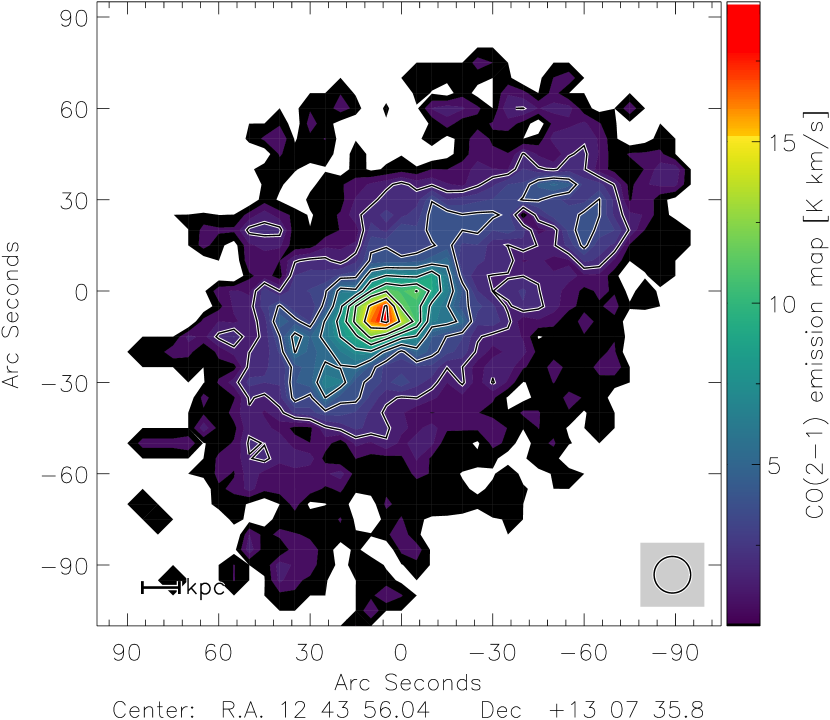
Figure 3: NGC 4654 CO(2-1) emission map. Contour levels are 2, 4, 6, 8, 10, 12, 15 and 18 K $\rm km\ s^{-1}$. The resolution is 12”.

As a consequence of the gravitational interaction between NGC 4654 and NGC 4369, the CO velocity field (Fig. 4) shows an asymmetric profile along the major axis, with a constant velocity plateau reached in the southeast that is absent in the northwest. We determine the systemic velocity at 1060 $\rm km\ s^{-1}$, measured in the optical center of the galaxy using $\rm{H\alpha}$ data from GOLDMINE (Gavazzi et al. 2003). This is consistent with the value of $1050\ \rm km\ s^{-1}$ given by the SDSS DR12 catalog (Alam et al. 2015). Considering 1060 $\rm km\ s^{-1}$, the maximum velocities reached in the southeast and the northwest regions are +150 $\rm km\ s^{-1}$ and -170 $\rm km\ s^{-1}$, respectively.

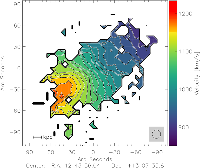
Figure 4: NGC 4654 CO(2-1) velocity field. Contours levels are from 900 to 1200 $\rm km\ s^{-1}$ in steps of 20 $\rm km\ s^{-1}$.

The position-velocity diagrams along the major and the minor axis of the galaxy are presented in Fig. 5. In the southeast, the behavior of the diagram is standard: a gradient around the center of the galaxy ending with a velocity plateau at 3 kpc. On the other hand, in the northwest, the plateau is reached at 2 kpc and is followed by a second gradient at 4 kpc. The position-velocity diagram along the minor axis does not show any strong asymmetry.

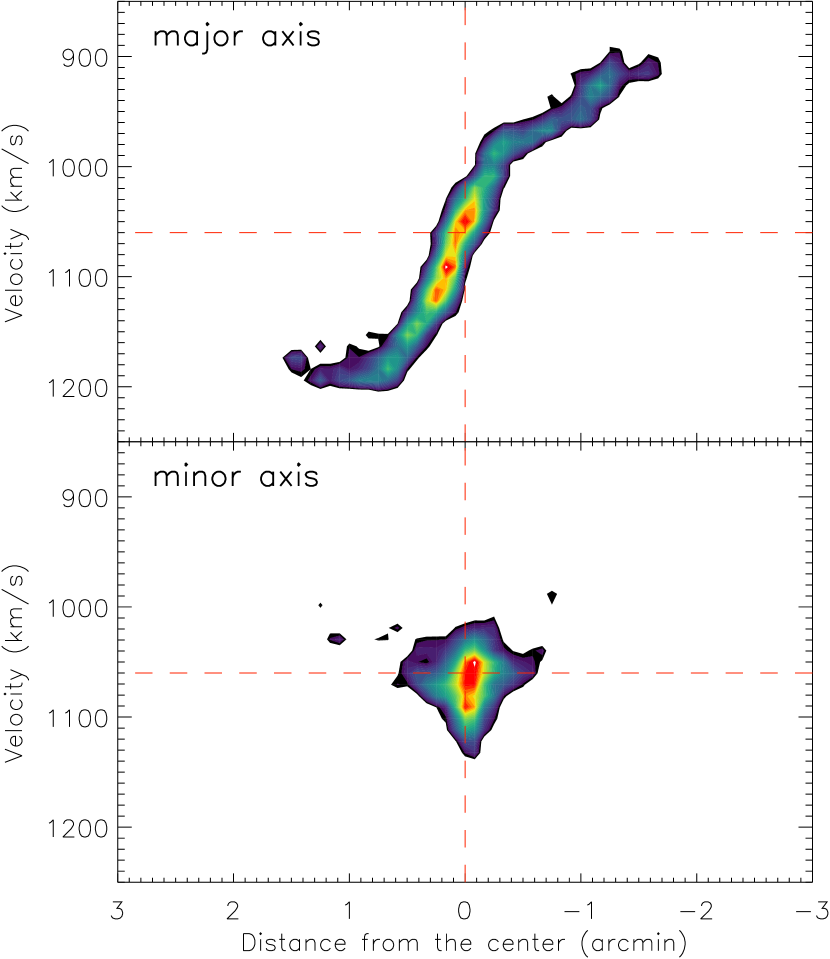
Figure 5: Position-velocity diagram of the CO(2-1) emission. Top panel: Along the major axis. Bottom panel: Along the minor axis. The dotted red line corresponds to the systemic velocity of 1060 $\rm km\ s^{-1}$.

The moment 2 map for the CO(2-1) data cube is presented in Fig. 6. Because of galactic rotation, the observed velocity dispersion strongly increases in the region around the center of the galaxy, with $\Delta\nu$ $\simeq$ 40 $\rm km\ s^{-1}$. In the northwestern high $\rm{H\textsc{i}}$ surface density region, the CO(2-1) linewidth is 5-10 $\rm km\ s^{-1}$ broader than in the inner arm between the $\rm{H\textsc{i}}$ region and the center of the galaxy.

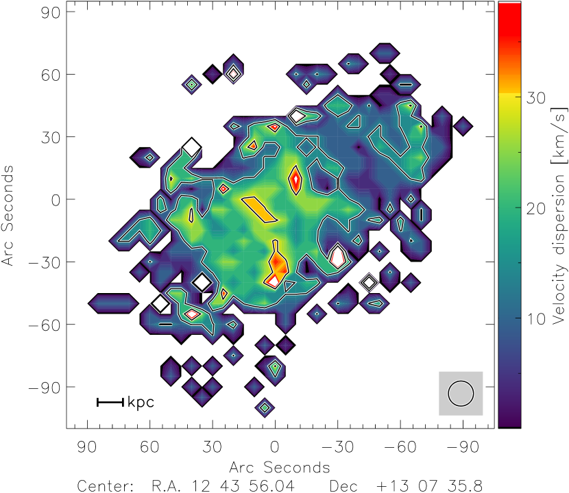
Figure 6: CO(2-1) moment 2 map. Contour levels correspond to 15 and 30 $\rm km\ s^{-1}$.

4 Ancillary data

In order to compute the SFR, the total gas and the ISM pressure, we used existing FUV 1528 Å data from GALEX (Martin et al. 2005), infrared 3.6$\rm{\mu m}$ and 24$\rm{\mu m}$ from SPITZER (Werner et al. 2004), $\rm{H\alpha}$ emission from GOLDMINE Gavazzi et al. (2003) and $\rm{H\textsc{i}}$ data from VIVA survey Chung et al. (2008). The above-mentioned data are presented in the following subsections :

4.1 Atomic gas

The atomic gas surface density $\rm{\Sigma_{\rm{HI}}}$ is obtained using the VLA $\rm{H\textsc{i}}$ data from Chung et al. (2008):

$$\frac{\Sigma_{\rm{HI}}}{(\rm{M_{\odot}pc^{-2}})}=0.020\ \frac{{I_{21cm}}}{(\rm{K\leavevmode\nobreak\ \rm km\ s^{-1}})}\leavevmode\nobreak\ ,$$ (1)

with ${I_{21cm}}$ converted from Jy/beam to K $\rm km\ s^{-1}$. The expression contains a coefficient of 1.36 to reflect the presence of Helium. The rms at 3 $\sigma$ is about 0.5 $\rm{M_{\odot}pc^{-2}}$ and the spatial resolution is 16”. The contour map of $\rm{\Sigma_{\rm{HI}}}$ is shown in Fig. 1. For the following sections, we will consider the $\rm{high\ H\textsc{i}\ surface\ density\ region}$ as the northwestern area where $\rm{\Sigma_{\rm{HI}}}$ ¿ 28 $\rm{M_{\odot}pc^{-2}}$.

4.2 Star-formation rate

Chung & Kim (2014) computed the SFR of NGC 4654 using the 1.4 GHz radio continuum data from the NRAO VLA Sky Survey (NVSS, Condon et al. 1998). However, the conversion between the radio continuum emission and SFR has a large scatter (Vollmer et al. 2020) and is uncertain in galaxies whose ISM is affected by ram pressure stripping (Murphy et al. 2006). We therefore use GALEX FUV all-sky survey (Martin et al. 2005) and SPITZER $24\rm{\mu}$m data (PI: J.D.P. Kenney) for the calculation of the star-formation map. We computed the SFR following Leroy et al. (2008):

$$\dot{\Sigma}_{\star}(FUV+24{\mu}m)=8.1\times 10^{-2}I_{FUV}+3.2\times 10^{-3}I_{24{\mu}m}\ ,$$ (2)

where $\dot{\Sigma}_{\star}(FUV+24\leavevmode\nobreak\ \rm{\mu}m)$ is the SFR in $\rm{M_{\odot}}$ kpc^-2 yr^-1 and $I_{FUV}$ and $I_{24\rm{\mu}m}$ are given in MJy/sr. The maximum of 0.27 $\rm{M_{\odot}}$ kpc^-2 yr^-1 is reached in the high atomic gas surface density region at the outer edge of the stellar arm. This value is 1.5 times higher than that of the galaxy center. The total integrated SFR is 1.84 $\rm{M_{\odot}}$yr^-1, which places NGC 4654 on the star-forming main sequence, considering its stellar mass (e.g, Brinchmann et al. 2004, Noeske et al. 2007, Daddi et al. 2007). The $\rm{high\ H\textsc{i}\ surface\ density\ region}$ concentrates 20% of the total SFR of NGC 4654 (0.37 $\rm{M_{\odot}}$kpc^-2yr^-1). The compact region of high star-formation, where $\rm{\dot{\Sigma}_{\star}}$ ¿ 0.20 $\rm{M_{\odot}}$kpc^-2yr^-1, accounts for 5% of the total SFR of NGC 4654 (0.09 $\rm{M_{\odot}}$kpc^-2yr^-1), which corresponds to $\sim$25% of the SFR in the entire $\rm{high\ H\textsc{i}\ surface\ density\ region}$.

Figure 7: Star-formation rate based on GALEX FUV and SPITZER 24 $\rm{\mu}m$ data. Contour levels correspond to 0.02, 0.05, 0.10, and 0.20 $\rm{M_{\odot}}$kpc^-2yr^-1. The resolution is 6”.

These results are consistent within 5% with the SFR computed using the $\rm{H\alpha}$ emission from GOLDMINE Gavazzi et al. (2003), following Leroy et al. (2008). A third method was tested, combining the FUV data with the TIR emission computed from the 3.6, 24 (SPITZER), 100 and 160$\rm{\mu}m$ flux (HERSCHEL). The method is described in Hao et al. (2011) and Galametz et al. (2013). The SFR_FUV+TIR shows slightly different results with a maximum of the SFR in the center of the galaxy. This is expected because the interstellar radiation field (ISRF), which heats the dust emitting in the infrared, contains a significant fraction of optical starlight. In the $\rm{high\ H\textsc{i}\ surface\ density\ region}$, $\dot{\Sigma}_{\star}(FUV+24\rm{\mu}m)$ is about 2 times higher than $\dot{\Sigma}_{\star}(FUV+TIR)$. The total integrated SFR using TIR as infrared contribution gives 1.53 $\rm{M_{\odot}}$yr^-1, which is 20% lower than the total SFR calculated from the FUV + 24 $\rm{\mu}m$ or $\rm{H\alpha}$ recipes.

4.3 Stellar surface density

The stellar surface density $\Sigma_{\star}$ is obtained from 3.6 $\rm{\mu}m$ SPITZER data following Leroy et al. (2008):

$$\frac{\Sigma_{\star}}{\rm{(M_{\odot}pc^{-2})}}=280\frac{I_{3.6\leavevmode\nobreak\ \rm{\mu}m}}{\rm{(MJy\leavevmode\nobreak\ sr^{-1})}}\leavevmode\nobreak\ .$$ (3)

The resulting map is presented in Fig. 1. The stellar surface density makes it possible to calculate the vertical stellar velocity dispersion, $v_{\rm{disp}}^{\star}$, necessary to estimate the ISM pressure of the disk:

$$v_{\rm{disp}}^{\star}=\sqrt{\Sigma_{\star}\frac{2\pi Gl_{\star}}{7.3}}\ ,$$ (4)

where $l_{\star}$ is the stellar scale length computed from the radial profile of the stellar surface density. To do so, we averaged the stellar surface density within ellipsoidal annuli of 0.6 kpc width and determined the slope in lin-log space. We obtained $l_{\star}$ = 2.3 kpc. The exponential stellar scale height is assumed constant with $l_{\star}$/$h_{\star}$ = 7.3 $\pm$ 2.2 (Kregel et al. 2002), corresponding to $h_{\star}\sim 0.3$ kpc.

5 CO-to-$\rm{H_{2}}$ conversion factor from dust emission

The CO-to-H₂ conversion factor is critical for our estimation of the molecular surface density and for the subsequent physical quantities of this study, the star-formation efficiency and the molecular fraction. For non-starburst spiral galaxies at low redshift, it is quite common to use the Milky Way standard value of $\rm{X_{\rm{CO}}^{\rm{MW}}}$ = 2 $\times$ 10²⁰ $\rm{cm^{-2}(K\ \rm km\ s^{-1})^{-1}}$ (e.g, Bolatto et al. 2013). In the following sections, we will use the equivalent expression of the conversion factor expressed in solar masses, $\rm{\alpha_{\rm{CO}}^{\rm{MW}}}$ = 4.36 $\rm{M_{\odot}(K\ \rm km\ s^{-1}\ pc^{2})^{-1}}$ that takes into account a factor of 1.36 for the presence of Helium.

Bolatto et al. (2013) suggested that below $\sim$1/2-1/3 of the solar metallicity, the conversion factor tends to increase significantly. Since the high $\rm{H\textsc{i}}$ surface density region is located close to the optical radius, where generally the metallicity is Z $\sim$ 1/2-1/3 Z_⊙, a higher conversion factor is not excluded in this region. Chung & Kim (2014) also suggested that the conversion factor in this region might be higher than the Galactic standard value. We estimated the CO-to-H₂ conversion factor using the hydrogen column density $N_{H}$ calculated from the far infrared HERSCHEL bands at 250$\rm{\mu}m$ and 350$\rm{\mu}m$ and the dust-to-gas ratio, DGR, by applying the method presented in Leroy et al. (2011). By combining the dust emission with the CO and $\rm{H\textsc{i}}$ data, the following equation can be established:

$$\frac{N_{\rm{H}}^{\rm{dust}}}{\eta}=N_{\rm{H}}^{\rm{HI}}+2\leavevmode\nobreak\ N_{\rm{H}}^{\rm{H_{2}}}=N_{\rm{H}}^{\rm{HI}}+2\leavevmode\nobreak\ X_{\rm{CO}}\leavevmode\nobreak\ I_{\rm{CO}}(1-0)\ ,$$ (5)

where $I_{CO(1-0)}$ is the CO(1-0) emission computed from the CO(2-1) emission assuming a line ratio $\rm{I_{CO(1-0)}=I_{CO(2-1)}/0.8}$ (Hasegawa 1997) and $\eta$ = DGR/DGR_⊙ is the DGR normalized by the solar DGR (DGR_⊙ $\sim$ 1/100, Draine et al. 2007). The use of $\eta$ introduces a metallicity dependence in the calculations. The optical depth is given by:

$$\tau_{\nu}=\int\sigma_{\nu}\leavevmode\nobreak\ N_{\rm{H}}\leavevmode\nobreak\ ds\ ,$$ (6)

where $\sigma_{\nu}$ is the absorption coefficient such that $\sigma_{\nu}$ $\propto$ $\nu\leavevmode\nobreak\ ^{\beta}$ with $\beta$ = 2. In order to calculate the column density, it is necessary to determine the temperature of the dust at each point of the galaxy using:

$$\frac{F_{250\rm{\mu}m}}{F_{350\rm{\mu}m}}=\frac{B_{250\rm{\mu}m}(T)}{B_{350\rm{\mu}m}(T)}\leavevmode\nobreak\ \left(\frac{\nu_{250\rm{\mu}m}}{\nu_{350\rm{\mu}m}}\right)^{\beta}\ ,$$ (7)

where $\rm{F_{250\mu m}}$ and $\rm{F_{250\mu m}}$ are the HERSCHEL fluxes and $\rm{B_{\nu}(T)}$ is a modified black-body function. The resulting map is shown in Fig. 8. The maximum of the dust temperature, reached in the galaxy center, is about 27 K. The dust is significantly warmer along the dense stellar arm than in the inter-arm region with a local maximum of 22 K in the $\rm{high\ H\textsc{i}\ surface\ density\ region}$. The temperature is 5 K higher in this region than in the rest of the disk at the same radius.

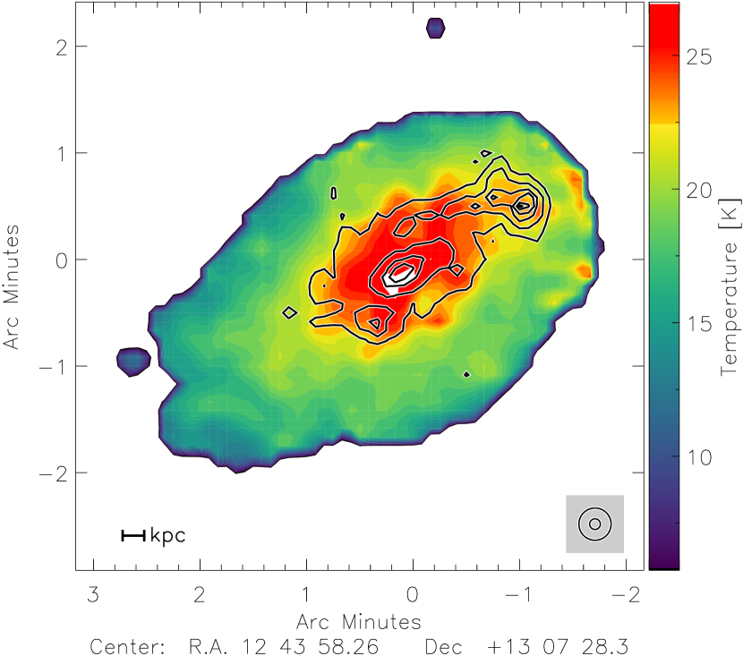
Figure 8: Dust temperature map based on HERSCHEL 250$\rm{\mu}m$ and 350$\rm{\mu}m$ data. Contour levels correspond to $\dot{\Sigma}_{\star}=$ 0.02, 0.05, 0.10, and 0.20 $\rm{M_{\odot}}$kpc^-2yr^-1.

The hydrogen column density is obtained using the 250 $\rm{\mu}$m band together with a dust absorption coefficient $\sigma_{250\rm{\mu}m}$:

$$N_{\rm{H}}^{\rm{dust}}=\frac{F_{250\rm{\mu}m}}{B_{250\rm{\mu}m}(T)\leavevmode\nobreak\ \sigma_{250\rm{\mu}m}}\ .$$ (8)

The dust absorption coefficient $\sigma_{250\rm{\mu}m}$ is calibrated in a region where no CO is detected (i.e, I_CO = 0) by combining Eq. 5 and Eq. 8:

$$\sigma_{250\rm{\mu}m}\leavevmode\nobreak\ \eta=\frac{F_{250\rm{\mu}m}}{B_{250\rm{\mu}m}(T)N_{\rm{H}}^{\rm{HI}}}\ .$$ (9)

At this point, we only determine the value of the product between $\eta$ and $\sigma_{250\rm{\mu}m}$ but not their respective contributions. For a comparison with the Galactic absorption coefficient, we assume that the DGR evolves linearly with the metallicity of the gas. Gordon et al. (2014) calculated the grain absorption cross section per unit mass $\kappa_{\lambda}$ using the Herschel HERITAGE survey (Meixner et al. 2014):

$$\kappa_{\lambda}=\kappa_{160\mu m}\ \left(\frac{\lambda}{160}\right)^{-\beta}\ ,$$ (10)

where $\kappa_{160\mu m}$ = 30.2 cm² g^-1 (SMBB model in Table 2 of Gordon et al. 2017). With a coefficient $\beta$ = 2, the solar neighborhood value within the Milky Way at 250 $\rm{\mu}m$ is $\kappa_{250\rm{\mu}m}^{\leavevmode\nobreak\ \rm{MW}}$ = 12.36 cm²g^-1. Eq. 9 and Eq. 10 lead to the relation:

$$\sigma_{250\rm{\mu}m}\ \eta=\left(\frac{Z}{Z_{\odot}}\right)\kappa_{250\rm{\mu}m}^{\leavevmode\nobreak\ \rm{MW}}m_{p}\rm{DGR}_{\odot}\ .$$ (11)

We calculated this ratio in regions without any CO detection and found metallicity of $\sim$1/2 Z_⊙ at 9 kpc from the galaxy center. This result is consistent with direct measurements of Skillman et al. (1996) in Fig. 10. We obtained $\sigma_{\rm{dust}}$ = 8.0 $\times$ 10^-26 cm², which is consistent with the standard value of 1.1 $\times$ 10^-25 cm² (Draine & Lee 1984). We used this value in Eq. 8. and computed the hydrogen column density from dust emission for the entire galactic disk.

Based on the assumption that the DGR varies only slightly at kpc-scale within galactic disks (Leroy et al. 2011, Sandstrom et al. 2013, ), the DGR and $\rm{X_{\rm{CO}}}$ can be simultaneously determined using Eq. 5. For given $\rm{I_{\rm{CO}}}$ and $\rm{\Sigma_{\rm{HI}}}$, the process consists in searching for the conversion factor that minimizes the dispersion of the DGR values in kiloparsec-size regions. We adopted the method suggested by Sandstrom et al. (2013): the study have to be carried out i) in areas where CO is detected; ii) within a range of conversion factors from 0.1-100 $\times$ 10²⁰ $\rm{cm^{-2}(K\ \rm km\ s^{-1})^{-1}}$; iii) by selecting regions containing 9 resolution elements. We defined four distinct regions in NGC 4654: a first ring around the galactic center at a distance of 2 kpc, a second ring from 2 to 3 kpc, a region that contain the northwest stellar arm and the $\rm{high\ H\textsc{i}\ surface\ density\ region}$. Fig. 9 presents the DGR minimization method for the $\rm{high\ H\textsc{i}\ surface\ density\ region}$. The other regions can be found in Appendix C.

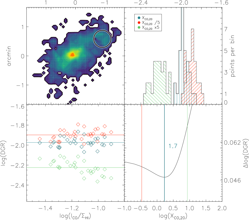
Figure 9: Simultaneous determination of the dust-to-gas ratio and the CO-to-$\rm{H_{2}}$ conversion factor based on method described in Sandstrom et al. (2013). Top-left panel: Selected region for the study on the CO(2-1) map. Top-right panel: Scatter of the DGR calculated within resolution elements inside the selected area for different X_CO. Bottom-left panel: Standard deviation of the DGR as a function of the ration between the CO(2-1) flux and the Hi gas surface density. Bottom-right panel: DGR dispersion as a function of X_CO.

The results of the DGR variation method for the four regions are presented in Table 2. The uncertainties in the DGRs are estimated via bootstrapping (see Sandstrom et al. 2013). All CO-to-H₂ conversion factors are consistent with the Galactic value within the errors.

Table 2: Results of the minimization of the DGR variation method.

	Central ring	Outer ring	Inner arm	$\rm Hi\Sigma_{HI}$
D [kpc]	2.0	2.9	5.1	6.3
$\alpha_{\rm CO}$	3.7 $\pm$ 1.2	3.3 $\pm$ 1.1	6.5 $\pm$ 0.6	3.7 $\pm$ 0.6
DGR/DGR⊙	1.2 $\pm$ 0.2	1.3 $\pm$ 0.2	0.9 $\pm$ 0.1	1.0 $\pm$ 0.1
12+log[O/H]	8.8 $\pm$ 0.1	8.8 $\pm$ 0.1	8.7 $\pm$ 0.1	8.7 $\pm$ 0.1

As the DGR is expected to depend linearly on metallicity, we compare the metallicity based on the DGR variations to direct measurements. Skillman et al. (1996) obtained 12+log[O/H] measurements using the strong-line method. For a reliable detection of the electronic temperature, the detection of faint auroral lines is necessary. However, Skillman et al. (1996) carried out the determination of the metallicity with a constant $\rm{T_{e}}$. By using a spectrum stacking method in regions where auroral lines are usually not detected, although necessary for metallicity measurements, Curti et al. (2017) were able to define a new mass-metallicity calibration (MZR) for star-forming galaxies. This new calibration reveals a systematic and significant offset for high mass galaxies. At the typical mass of NGC 4654, this offset is about 0.3 dex below previous calibrations (see Curti et al. 2020). We therefore recalibrated the data from Skillman et al. (1996) by applying this offset. A second recalibration was performed based on the work of Pérez-Montero & Contini (2009) (PMC09). This recalibration consists in the estimation of the metallicity

$$\rm 12+log[O/H]=8.74-0.31\times O3N2$$ (12)

with the O3N2 ratio

$$\rm O3N2=log\left[\frac{I[OIII]\ (5007\AA)}{I[{H\beta}]}\times\frac{I[H\alpha]}{I[NII](6584\AA)}\right]$$ (13)

derived from the data of Skillman et al. (1996).

The Skillman et al. (1996) metallicity profiles recalibrated following Curti et al. (2020) and PMC09 are compared to the metallicity profile determined by the DGR method in Fig. 10. These methods lead to metallicities close to the solar value (see Table 2). The Curti et al. (2020) and PMC09 recalibrations resulted in metallicity gradients of $-0.07$ dex/kpc and $-0.05$ dex/kpc, respectively (Fig. 10). Both profiles lead to a solar metallicity at the distance of 4.5 kpc.

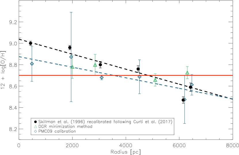
Figure 10: Radial profile of the metallicity (12+log[O/H]). The strong-line method measurements from Skillman et al. (1996) corrected following Curti et al. (2020) are shown in black. The PMC09 recalibration is shown in blue. The minimization of the DGR variation is shown in green. The solar metallicity $\rm(12+log[O/H])_{\odot}=8.7$ is shown in red.

An alternative CO-to-H₂ conversion factor can be obtained by converting the recalibrated metallicities to DGRs. The $\rm{X_{\rm{CO}}}$ derived from Eq. 5 are presented in Fig. 11. Between 0 and 5 kpc the mean CO-to-H₂ conversion factors are $\rm{\alpha_{\rm{CO}}}$ = 3.9 $\rm{M_{\odot}(K\ \rm km\ s^{-1}\ pc^{2})^{-1}}$ for the Curti et al. (2020) recalibration and $\rm{\alpha_{\rm{CO}}}$ = 5.7 $\rm{M_{\odot}(K\ \rm km\ s^{-1}\ pc^{2})^{-1}}$ for the PMC09 recalibration. These values are close to the Galactic conversion factor. The conversion factors in the $\rm{high\ H\textsc{i}\ surface\ density\ region}$ are $\rm{\alpha_{\rm{CO}}}$ $\sim$ 8.2 $\rm{M_{\odot}(K\ \rm km\ s^{-1}\ pc^{2})^{-1}}$ and $\rm{\alpha_{\rm{CO}}}$ $\sim$ 8.7 $\rm{M_{\odot}(K\ \rm km\ s^{-1}\ pc^{2})^{-1}}$, about twice the Galactic value. We therefore set $\rm{\alpha_{\rm{CO}}}$ = 2 $\rm{\alpha_{\rm{CO}}^{\rm{MW}}}$ in the high $\rm{H\textsc{i}}$ surface density region and $\rm{\alpha_{\rm{CO}}}$ = $\rm{\alpha_{\rm{CO}}^{\rm{MW}}}$ otherwise. The maps presented in the following sections are based on this modified conversion factor. The same maps for a Galactic conversion factor, $\rm{\alpha_{\rm{CO}}^{\rm{MW}}}$  in the $\rm{high\ H\textsc{i}\ surface\ density\ region}$ are presented in Appendix D.

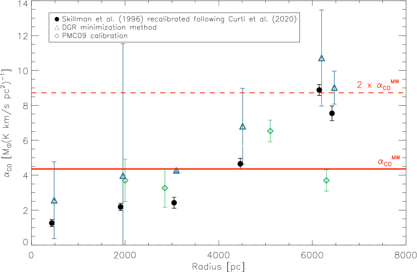
Figure 11: Radial profile of the CO-to-H₂ conversion factor. The red line corresponds to the Galactic conversion factor $\alpha_{\rm{CO}}^{\rm{MW}}$ = 4.36 M_⊙(K $\rm km\ s^{-1}$ pc²)^-1. Black dots correspond to the $\rm{\alpha_{\rm{CO}}}$ estimation using Skillman et al. (1996) metallicities. Black triangles correspond to the conversion factors estimated using the DGR dispersion minimization method.

6 Molecular and total gas

The molecular gas surface density is computed using the CO-to-H₂ conversion factor presented in Sect. 5. and is given by the following equation:

$$\Sigma_{\rm{H_{2}}}=\alpha_{\rm{CO}}\ \frac{I_{\rm{CO}}(2-1)}{0.8}\ .$$ (14)

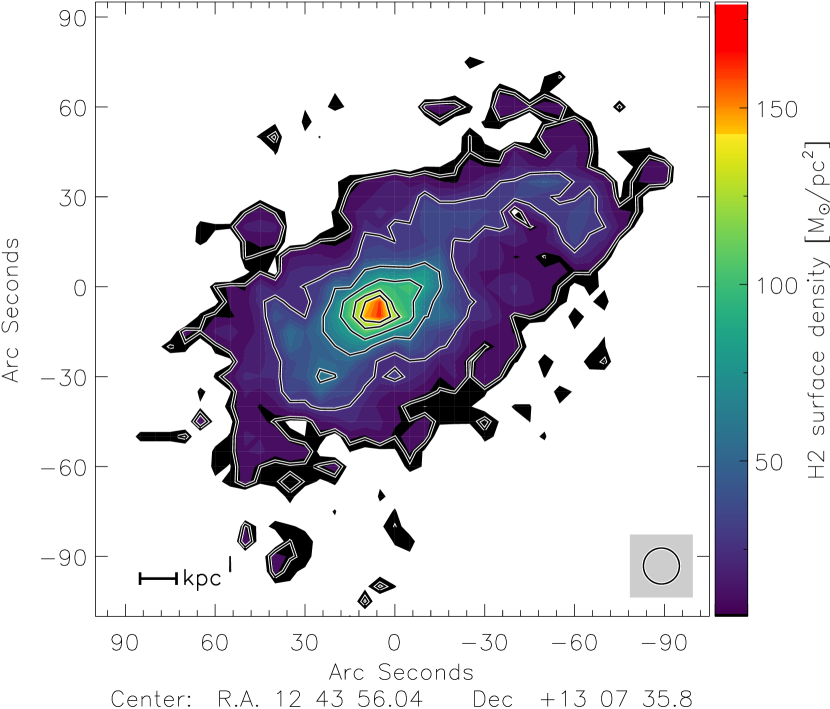
Figure 36: Molecular gas surface density. Contours levels are 10, 30, 60, 90, 120, and 140 $M_{\odot}pc^{-2}$. The resolution is 12”.

A factor of 1.36 reflecting the presence of Helium is included in $\rm{\alpha_{\rm{CO}}}$. The 3$\sigma$ detection limit of the CO data is $0.5$ $\rm{M_{\odot}pc^{-2}}$ for a constant channel width of 10.4 $\rm km\ s^{-1}$. The resulting map is presented in Fig. 12. using the modified $\alpha_{\rm{CO}}$ conversion factor and in Fig. 36 with a constant $\rm{\alpha_{\rm{CO}}^{\rm{MW}}}$. The maximum of the molecular gas surface density is reached in the galaxy center, $\rm{\Sigma_{\rm{H_{2}}}}$ = 173 $\rm{M_{\odot}pc^{-2}}$. The distribution of the molecular gas is strongly asymmetric along the major axis, extended to $\sim$1.6’ (7 kpc) to the southeast and $\sim$1.8’ (8 kpc) to the northwest. Toward the northwest, a high molecular gas surface density arm at 40-50 $\rm{M_{\odot}pc^{-2}}$ is detected, following the stellar arm (Fig. 1.). The surface density values along the arm are 2 to 3 times higher than in the inter-arm region. Within the $\rm{high\ H\textsc{i}\ surface\ density\ region}$, where the conversion factor is assumed to be 2 $\times$ $\rm{\alpha_{\rm{CO}}^{\rm{MW}}}$, the maximum value is $\rm{\Sigma_{\rm{H_{2}}}}$ = 99 $\rm{M_{\odot}pc^{-2}}$. The total molecular gas mass is $\rm{M_{\rm{H_{2}}}}$ = 2.1 $\times$ 10⁹ $\rm{M_{\odot}}$, which is about 10% higher than the value using a constant $\rm{\alpha_{\rm{CO}}^{\rm{MW}}}$.

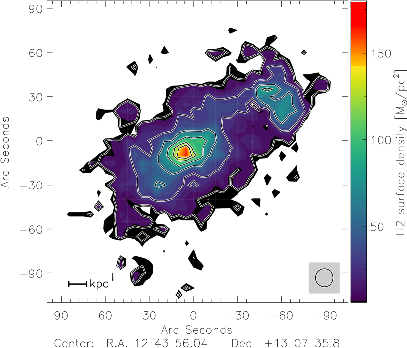
Figure 12: H₂ surface density. Contour levels are $10$, $30$, $60$, $90$, $120$ and $140$ $\rm{M_{\odot}pc^{-2}}$. The resolution is 12”.

Convolved to the spatial resolution of 16”, the molecular surface density can be added to the atomic surface density to compute the total gas map (Fig. 13). The maximum gas surface density is reached in the galaxy center with $\rm{\Sigma_{\rm{gas}}=154\ M_{\odot}pc^{-2}}$, which is lower than the value presented for $\rm{H_{2}}$ due to the convolution of the data. Along the spiral arm toward the northwest, the density is approximately constant, $\rm{\Sigma_{\rm{gas}}=60-70\ M_{\odot}pc^{-2}}$. Within the $\rm{high\ H\textsc{i}\ surface\ density\ region}$, a local maximum of 117 $\rm{M_{\odot}pc^{-2}}$ is observed.

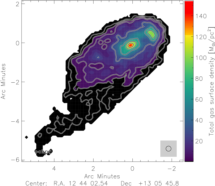
Figure 13: Total gas surface density $\Sigma_{\rm gas}=\Sigma_{\rm{HI}}+\Sigma_{\rm{H_{2}}}$. Contour levels are 2, 5, 10, 30, 60, 90 and 120 $\rm{M_{\odot}pc^{-2}}$. The resolution is 16”.

7 Molecular fraction and pressure

The molecular fraction corresponds to the ratio of the molecular surface density divided by the atomic surface density, $\rm{R_{\rm{mol}}=\Sigma_{\rm{H_{2}}}/\Sigma_{\rm{HI}}}$ (Fig. 14). The molecular fraction reaches its maximum in the galaxy center, where $R_{\rm{mol}}$ = 8-9. Within the disk of NGC 4654, $R_{\rm{mol}}$ decreases with increasing radius. In the $\rm{high\ H\textsc{i}\ surface\ density\ region}$, the molecular fraction is 2-3 times higher than in the disk at the same radius, reaching a local maximum, $\rm{R_{\rm{mol}}\sim 2}$.

Figure 14: Molecular fraction $R_{\rm{mol}}$ = $\Sigma_{\rm{H_{2}}}$ / $\Sigma_{\rm{HI}}$. Contours levels are 0.5, 1, 2, 4 and 7. The resolution is 16”.

Blitz & Rosolowsky (2006) found a close correlation between the molecular fraction and the total gas mid-plane pressure in the star-forming galaxies, such that $R_{\rm{mol}}$ = $P^{0.92\pm 0.07}_{\rm{tot}}$. Assuming hydrostatic equilibrium within the disk, the total mid-plane pressure is computed following Elmegreen (1989):

$$P_{\rm{tot}}=P_{\rm{gas}}+P_{\star}=\left(\frac{\pi}{2}G\Sigma_{\rm{gas}}^{2}\right)+\left(\frac{\pi}{2}G\Sigma_{\rm{gas}}\Sigma_{\star}\frac{v_{\rm{disp}}}{v_{\rm{disp}}^{\star}}\right)\ ,$$ (15)

where G is the gravitational constant and $v_{\rm{disp}}$ the gas velocity dispersion $v_{\rm disp}=10(\pm 2)$ km s^-1 (Tamburro et al. 2009). The resulting map is shown in Fig. 15, the ratio between $P_{\rm gas}$ and $P_{\star}$ is presented in Fig. 30. The general distribution of the pressure within the disk is similar to that of the molecular fraction, with a global maximum at the galaxy center and a local maximum in the $\rm{high\ H\textsc{i}\ surface\ density\ region}$. The relation between the molecular fraction and the ISM pressure is presented in Fig. 16.

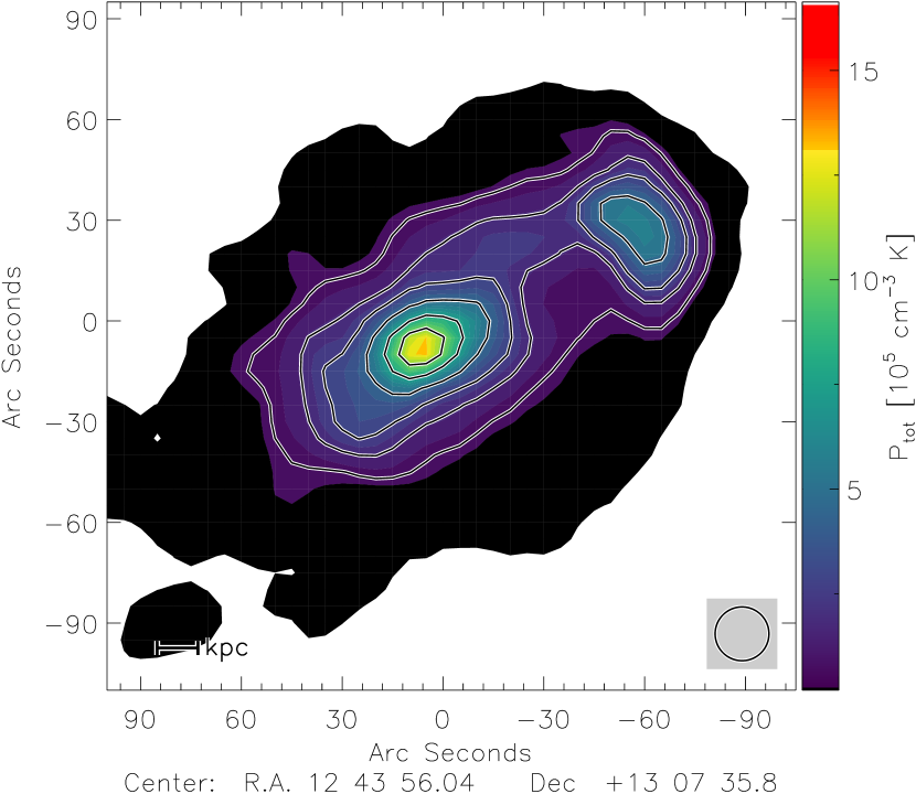
Figure 15: Total ISM mid-plane pressure. Contours levels are 1, 2, 3, 5, 8 and 11 $\times$ 10⁵ cm^-3 K. The resolution is 16”.

The slope of the correlation between $R_{\rm{mol}}$ and $\rm{P_{\rm{tot}}}$ is (1.00 $\pm$ 0.18). This result is consistent with the the value reported by Blitz & Rosolowsky (2006) cited above. However, the points corresponding to the $\rm{high\ H\textsc{i}\ surface\ density\ region}$ deviate from the correlation. These values are about 2-3 $\sigma$ lower than expected by the linear correlation. For a constant $\rm{\alpha_{\rm{CO}}^{\rm{MW}}}$, this offset is still present because both $R_{\rm{mol}}$ and $\rm{P_{\rm{tot}}}$ depend on $\rm{\Sigma_{\rm{H_{2}}}}$. By decreasing the conversion factor the points corresponding the high HI surface density move parallel to the correlation. We conclude that the lower $\rm{R_{\rm{mol}}/P_{\rm{tot}}}$ ratio in the $\rm{high\ H\textsc{i}\ surface\ density\ region}$ is independent of the choice of $\rm{\alpha_{\rm{CO}}}$.

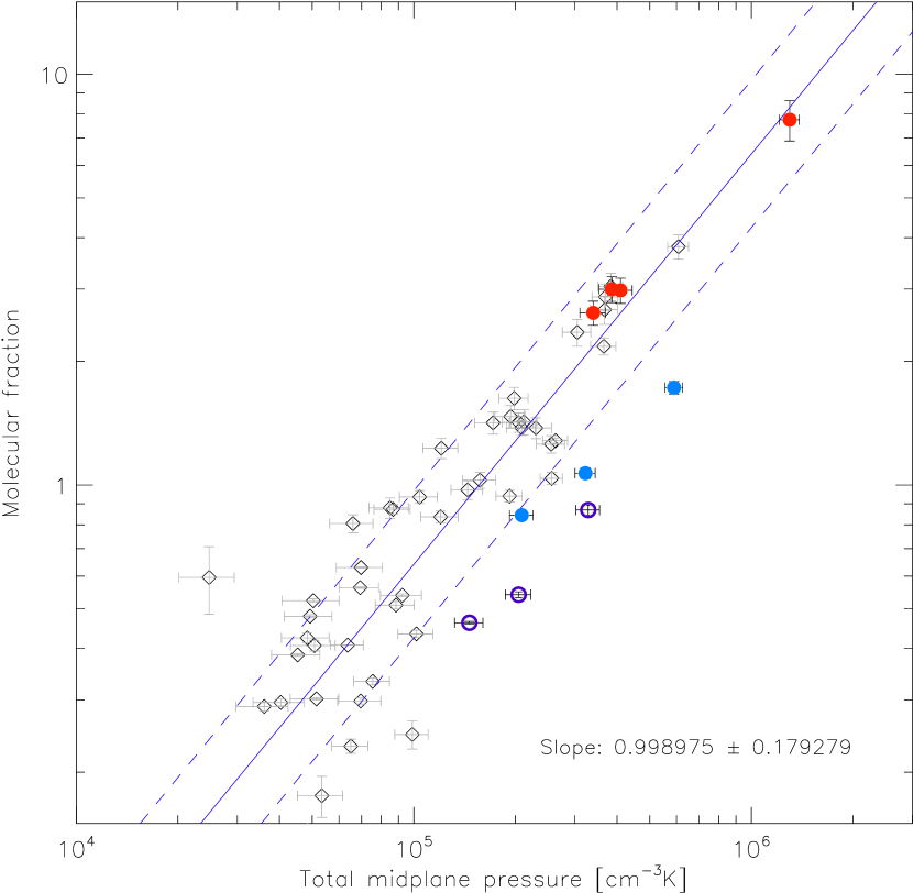
Figure 16: Molecular fraction $R_{\rm{mol}}$ as a function of the ISM pressure $P_{\rm{tot}}$. Light blue points correspond to the high HI surface density region with $\rm{\alpha_{\rm{CO}}}$= 2 $\times$ $\rm{\alpha_{\rm{CO}}^{\rm{MW}}}$. Dark blue circles correspond $\rm{\alpha_{\rm{CO}}}$= $\rm{\alpha_{\rm{CO}}^{\rm{MW}}}$. Red points correspond to the galaxy center. The dashed lines correspond to $\pm$ 1 $\sigma$.

8 Star-formation efficiency

Since molecular gas is closely correlated with star-formation, the study of cases where the $\rm{SFE_{\rm{H_{2}}}=\dot{\Sigma}_{\star}/\Sigma_{\rm{H_{2}}}}$ is not constant provide valuable information on the physics of the ISM. Bigiel et al. (2008) showed that variations of the star-formation efficiency within a galaxy are lower than those between individual galaxies. Chung & Kim (2014) suggested that the $\rm{SFE_{\rm{H_{2}}}}$ is significantly higher in the $\rm{high\ H\textsc{i}\ surface\ density\ region}$ than in the rest of the disk. We convolved the maps presented in Figs. 7 and 12 to a resolution of 12” to obtain the $\rm{SFE_{\rm{H_{2}}}}$ map shown in Fig. 17.

The molecular gas depletion timescale is defined as $\rm{\tau_{depl}^{\rm{H_{2}}}=SFE_{\rm{H_{2}}}^{-1}}$. The mean value within the galactic disk is $\rm{\tau_{depl}^{\rm{H_{2}}}}=\rm 1.5\ Gyr$, and $\rm{\tau_{depl}^{\rm{H_{2}}}}=\rm 2\ Gyr$ if we exclude the $\rm{high\ H\textsc{i}\ surface\ density\ region}$ in the calculations. The maximum of the star-formation efficiency is reached in the $\rm{high\ H\textsc{i}\ surface\ density\ region}$, where $\tau_{\rm depl}^{\rm{H_{2}}}$ $\sim$ 500 Myr, which is three times shorter than the mean value within the disk.

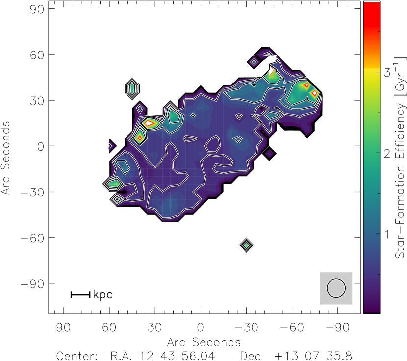
Figure 17: Star-formation efficiency with respect to the molecular gas. Contours levels are 0.5, 1 and 1.5 Gyr^-1. The resolution is 12”.

The SFR as a function of the molecular gas surface density is presented in Fig. 18. A linear power law is observed between the two quantities for NGC 4654, with a slope of 1.02 $\pm$ 0.18 in agreement with Bigiel et al. (2008) ($\rm{\dot{\Sigma}_{\star}}$ $\propto\Sigma^{1.0\pm 0.2}_{\rm{H_{2}}}$). The star formation efficiency of the galaxy center slightly is marginally lower by approximately 0.5 $\sigma$. For the modified $\rm{\alpha_{\rm{CO}}}$, the $\rm{SFE_{\rm{H_{2}}}}$ of three resolution elements within the $\rm{high\ H\textsc{i}\ surface\ density\ region}$ are 1-2 $\sigma$ higher than those of the rest of the disk. With a constant $\rm{\alpha_{\rm{CO}}^{\rm{MW}}}$, the $\rm{SFE_{\rm{H_{2}}}}$ of the same resolution elements are 2-3 $\sigma$ higher than their values expected from the linear correlation. Two other resolution elements within the $\rm{high\ H\textsc{i}\ surface\ density\ region}$ show values consistent with the linear correlation. These resolution elements are located at the northern edge of the $\rm{high\ H\textsc{i}\ surface\ density\ region}$.

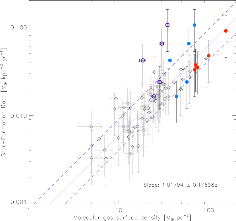
Figure 18: Star-formation rate $\rm{\dot{\Sigma}_{\star}}$ as a function of the molecular gas surface density $\rm{\Sigma_{\rm{H_{2}}}}$. Light blue points correspond to the high $\rm{H\textsc{I}}$ surface density region with $\rm{\alpha_{\rm{CO}}}$= 2 $\times$ $\rm{\alpha_{\rm{CO}}^{\rm{MW}}}$. Dark blue circles correspond to $\rm{\alpha_{\rm{CO}}}$= $\rm{\alpha_{\rm{CO}}^{\rm{MW}}}$. Red points corresponds to the galaxy center. The dashed lines correspond to $\pm$ 1 $\sigma$.

9 The Toomre stability criterion

The Toomre stability criterion (Toomre 1964) describes the stability of a gas disk against fragmentation. This criterion depends on the surface density and the velocity dispersion of both gas and stars. For our purpose we only evaluate the Toomre $Q$ parameter of the gas disk. Since the combined Toomre $Q$ parameter is always lower than the individual $Q$ parameters, the $Q$ parameter based on the gas can be regarded as an upper limit of the total $Q$ parameter. We use the Toomre criterion to evaluate if the northwestern region remains stable (Q $\geq$ 1) with an enhanced $\rm{\alpha_{\rm{CO}}}$. The Toomre $Q$ for the gas is calculated from the following equation (Toomre 1964):

$$Q_{\rm{gas}}=\frac{\kappa v_{\rm{disp}}}{\pi G\Sigma_{\rm{gas}}}\ ,$$ (16)

where $\kappa$ is the epicyclic frequency:

$$\kappa=\sqrt{2\ \frac{\Omega(R)}{R}\ \frac{d(R^{2}\Omega)}{dR}}\ .$$ (17)

The angular velocity is $\Omega$(R) = $\rm{v_{\rm{rot}}(R)/R}$ and $v_{\rm{rot}}$ is the rotation velocity of the galactic disk. We assume a constant gas velocity dispersion of $v_{\rm disp}=10(\pm 2)$ km s^-1 (Tamburro et al. 2009). In Sect. 10.1 this assumption is dropped and a radial profile of the velocity dispersion is calculated based on the analytical model of Vollmer (2003). We generated two different Toomre $Q$ maps. The first one is based on an approximation of the rotation curve following Boissier et al. (2003):

$$v_{\rm{rot}}=v_{\rm{flat}}\left(1-\rm{exp}\left(\frac{-R}{l_{\rm{flat}}}\right)\right)\ ,$$ (18)

where $l_{\rm{flat}}$ and $v_{\rm{flat}}$ represent the length scale and velocity at which the rotation curve becomes flat. We estimated both values from the position-velocity diagram presented in Fig. 5. The resulting map is shown in Fig. 19. The second Toomre $Q$ map is based on rotation velocities calculated from the deprojected CO velocity field (Fig. 39).

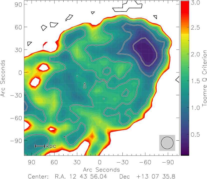
Figure 19: The Toomre $Q$ parameter. Contour levels are 0.5, 1, and 1.5.

The Toomre $Q$ parameter is lower than one in the whole disk except in the $\rm{high\ H\textsc{i}\ surface\ density\ region}$: the minimum is Q = $0.5$ for $\rm{\alpha_{\rm{CO}}^{\rm{MW}}}$ and Q = $0.3$ for the modified $\rm{\alpha_{\rm{CO}}}$.

10 Modeling NGC 4654

Our modeling effort is based on the combination of a small-scale analytical model together with a large-scale dynamical model, to handle the properties of a turbulent ISM in a simplified way. The analytical model takes into account gas pressure equilibrium (Eq. 15), molecule formation, the influence of self-gravity of giant molecular clouds, and stellar feedback. The large-scale dynamical model includes the gravitational interaction and ram pressure stripping. It gives access to the gas distribution and dynamics on scales of about $1$ kpc. The large-scale model does not include stellar feedback. The combination of the two models gives insight into the physics of the compressed ISM and its ability to form stars.

10.1 Analytical model

The analytical model used for this study is presented in detail in Vollmer & Leroy (2011). The analytical model describes a star-forming turbulent clumpy gas disk with a given Toomre $Q$, where the energy flux produced by supernova explosions is dissipated by the turbulence of the gas. This model generates radial profiles of the main quantities of this study ($\Sigma_{\rm{gas}}$, $\Sigma_{\rm{H_{2}}}$, $\Sigma_{\rm{HI}}$ and $\dot{\Sigma}_{\star}$) that can be compared with the observations to constrain its free parameters. The observational input parameters are the total stellar mass, the scale length of the stellar disk, and the rotation curve of the galaxy. In this model the ISM is considered as a single turbulent gas in vertical hydrostatic equilibrium:

$$p_{\rm{turb}}=\rho v_{\rm{turb}}^{2}=\frac{\pi}{2}G\Sigma_{\rm{gas}}\left(\Sigma_{\rm{gas}}+\Sigma_{\star}\frac{v_{\rm{turb}}}{v_{\rm{disp}}^{\star}}\right)\ .$$ (19)

Turbulence is driven by supernova explosions, which inject their energy into the ISM. The model considers turbulence as eddies with the largest eddies defined by a characteristic turbulent driving scale length $l_{\rm{driv}}$ and the associated velocity dispersion $v_{\rm{turb}}$. Assuming a constant initial mass function independent of environment, the following equation can be written:

$$\xi\dot{\Sigma}_{\star}=\Sigma_{\rm{gas}}\frac{v_{\rm{turb}}^{3}}{l_{\rm{driv}}}=\Sigma_{\rm{gas}}\nu\frac{v_{\rm{turb}}^{2}}{l_{\rm{driv}}^{2}}\ ,$$ (20)

where $\rm{\xi=4.6\times 10^{-8}(pc/yr)^{2}}$ is the constant relating the SNe energy input into star-formation (Vollmer & Beckert 2003). Turbulence gives also rise to the viscosity $\nu$ such that $\nu=v_{\rm{turb}}l_{\rm{driv}}$. In the model, the turbulent crossing time of a single cloud is compared to the gravitational free fall time in order to derive an expression of the volume filling factor $\phi_{\rm{v}}$. Self-gravitation can be assumed for clouds if the condition $\tau_{\rm{turb}}^{\rm{cl}}=\tau_{\rm{ff}}^{\rm{cl}}$ is verified. In such a case, the volume filling factor $\phi_{\rm{v}}$ links the average density of the disk $\rho$ to the density of individual clouds $\rho_{\rm{cl}}$ such that $\rho_{\rm{cl}}=\phi_{\rm{v}}^{-1}\rho$. The density of a single cloud $\rho_{\rm{cl}}$ refers to the density of the largest self-gravitating structures of a size $l_{\rm{cl}}$. The latter size is smaller than the driving length scale $l_{\rm{driv}}$ by a factor $\delta$, such that $l_{\rm{cl}}=l_{\rm driv}/\delta$. For self-gravitating clouds, the turbulent crossing time and the free-fall timescale can be written:

$$\tau_{\rm{turb}}^{\rm{cl}}=\delta^{-1}\frac{l_{\rm{driv}}}{v_{\rm{turb}}}\ ,$$ (21)

$$\tau_{\rm{ff}}^{\rm{cl}}=\sqrt{\frac{3\pi}{32G\rho_{\rm{cl}}}}\ .$$ (22)

These timescales are used to control both the balance between the atomic and molecular gas phases and between turbulence and star-formation. Considering clouds self-gravitation, the star-formation can be finally defined as:

$$\dot{\Sigma}_{\star}=\phi_{\rm{v}}\frac{\rho}{\tau_{\rm{ff}}}l_{\rm{driv}}=\delta\phi_{\rm{v}}\rho v_{\rm{turb}}\ .$$ (23)

In the model, the turbulent motion is expected to redistribute angular momentum in the gas disk like an effective viscosity would do. With this consideration, accretion toward the center is allowed and one can treat the galaxy disk as an accretion disk. Assuming a continuous and nonzero external gas mass accretion rate $\dot{\Sigma}_{\rm{ext}}$, the global viscous evolution can thus be written as:

$$\frac{\partial\Sigma_{\rm{gas}}}{\partial t}\sim\frac{\nu\Sigma_{\rm{gas}}}{R^{2}}-\dot{\Sigma}_{\star}+\dot{\Sigma}_{\rm{ext}}\ .$$ (24)

The mass accretion rate at a given radius in a galactic disk with a constant rotation curve is given by

$$\dot{M}(R)=-2\,\pi R\Sigma v_{\rm r}=4\pi R^{\frac{1}{2}}\frac{\nabla}{\nabla\,R}(\nu\Sigma R^{\frac{1}{2}})\ ,$$ (25)

where $v_{r}$ is the radial velocity. If a stable total Toomre criterion Q_tot $\sim$ 1 is held over a few rotation periods by the balance between the mass accretion rate and the gas loss due to star-formation, the galaxy disk can be considered as stationary, such that $\partial\Sigma$/$\partial t$ $\sim$ 0. For such a stationary gas disk, the local mass and momentum conservation yield:

$$\nu\Sigma_{\rm{gas}}=\frac{\rm{\dot{M}}}{2\pi}\ .$$ (26)

Since NGC 4654 underwent a tidal interaction about $500$ Myr ago and is now undergoing ram pressure stripping, it cannot be considered as a stable disk. However, the relatively unperturbed southeastern half of the disk of NGC 4654 is actually not far from such an equilibrium with a constant mass accretion rate (left panels of Fig. 20). On the other hand, the mass accretion rate clearly has to vary in the perturbed northwestern half of the disk. We decided to keep Eq. 26 for convenience and to radially vary $\dot{M}$. For each model, the real mass accretion rate can be calculated via Eq. 25.

The separation between the atomic and molecular phase of the ISM is defined by the molecular fraction, estimated by the ratio of the free-fall timescale to the molecule formation timescale (Eq. 22 and Eq. 28):

$$R_{\rm{mol}}=\frac{\Sigma_{\rm{H_{2}}}}{\Sigma_{\rm{HI}}}\simeq\frac{\tau_{\rm{ff}}^{\rm{cl}}}{\tau_{\rm{mol}}^{\rm{cl}}}\ ,$$ (27)

where the molecule formation timescale is:

$$\tau_{\rm{mol}}^{\rm{cl}}=\frac{\gamma}{\phi_{\rm{v}}^{-1}\rho}\ .$$ (28)

The factor $\gamma$ corresponds to the coefficient of molecule formation timescale (Tielens & Hollenbach 1985). If we assume no exchange between the ISM and the environment of the galaxy, we can estimate $\gamma$ based on a closed box model following Vollmer & Leroy (2011):

$$\gamma=\gamma_{0}\ \left(\ln\left(\frac{\Sigma_{\rm{gas}}+\Sigma_{\star}}{\Sigma_{\rm{gas}}}\right)\right)^{-1},$$ (29)

where $\gamma_{0}$ = 7.2 $\times$ 10⁷ $\rm{yr\ M_{\odot}\ pc^{-3}}$. The metallicity $Z$ can be estimated using the solar value of the constant of molecule formation $\gamma_{\odot}=4.7\times 10^{7}\ \rm{yr\ M_{\odot}\ pc^{-3}}$ as $\rm{Z/Z_{\odot}=(\gamma/\gamma_{\odot})^{-1}}$. In order to verify whether this approach is compatible with the results previously obtained using the strong-line method and the DGR variation method presented in Sect. 5, we used the radial profiles of the stellar and total gas surface densities to calculate the profile of the gas metallicity. We separated the galactic disk into two halves: (i) the unperturbed eastern half and (ii) the western half containing the $\rm{high\ H\textsc{i}\ surface\ density\ region}$. For the northwestern region, we separated two distinct cases: a constant conversion factor $\rm{\alpha_{\rm{CO}}^{\rm{MW}}}$ and the modified $\rm{\alpha_{\rm{CO}}}$ in the $\rm{high\ H\textsc{i}\ surface\ density\ region}$. The three resulting metallicity profiles are shown in Fig. 35. As the results obtained for both conversion factor assumptions are consistent with the previous metallicity estimates based on both, the recalibrated Skillman et al. (1996) observations and the DGR variation method, we conclude that the closed-box model is consistent with observations. Using the molecular fraction computed from Eq. 27, we obtained:

$$\Sigma_{\rm{H_{2}}}=\Sigma_{\rm{gas}}\ f_{\rm{mol}}=\Sigma_{\rm{gas}}\left(\frac{\Sigma_{\rm{H_{2}}}}{\Sigma_{\rm{H_{2}}}+\Sigma_{\rm{HI}}}\right)=\Sigma_{\rm{gas}}\left(\frac{R_{\rm{mol}}}{1+R_{\rm{mol}}}\right)\ ,$$ (30)

$$\Sigma_{\rm{HI}}=\Sigma_{\rm{gas}}\ (1-f_{\rm{mol}})=\Sigma_{\rm{gas}}\left(\frac{1}{1+R_{\rm{mol}}}\right)\ .$$ (31)

10.1.1 Additional free parameters

The three free parameters of the analytical model that can be varied to reproduce the observational profiles are: the scaling factor between driving and dissipation length scale $\delta$, the Toomre stability parameter $Q$, and the accretion rate $\dot{M}$. The modification of these parameters induces significant changes in the resulting model profiles: (i) an increase in $\rm{\dot{M}}$ leads to an increase in the gas velocity dispersion; (ii) a decrease in the Toomre $Q$ parameter leads to an increase in the gas surface density; (iii) an increasing $\delta$ leads to an increase in both, $R_{\rm{mol}}$ and $\rm{\dot{\Sigma}_{\star}}$.

In addition to the free parameters $\delta$, $Q$ and $\dot{M}$, we decided to vary three other parameters that have a significant impact on the radial profiles of the model: the constant relating the supernova energy injection rate to the SFR $\xi$, the stellar vertical velocity dispersion $v_{\rm{disp}}^{\star}$, and the constant of molecule formation timescale $\gamma_{0}$. Varying these parameters has several consequences on the radial profiles generated by the model: (i) an increase in $\xi$ induces a decrease in the SFR (see Eq. 20); (ii) a higher $v_{\rm{disp}}^{\star}$ leads to a lower SFR profile; (iii) an increase in $\gamma_{0}$ strongly decreases the molecular fraction, which means that the $\rm{H_{2}}$ radial profile is lowered and the $\rm{H\textsc{i}}$ radial profile is augmented.

10.1.2 Degeneracies between parameters

The study of the analytical model revealed degeneracies between the free parameters. A decrease in $Q$ or an increase in $\dot{M}$ both result in an higher gas surface density. To decrease the value of $R_{\rm{mol}}$, $\delta$ or $\gamma_{0}$ have to be increased. Finally, four of the six free parameters have a significant impact on the SFR profile: $\dot{M}$ positively; $\delta$, $\xi$ and $v_{disp}$ negatively.

10.1.3 Results

To determine which set of parameters best fits the observational data, we carried out two successive reduced-$\upchi^{2}$ minimizations: the first stage consists in the reproduction of the radial profiles averaged over the disk, excluding the northwest region, which differs from the rest. Once these parameters have been defined, a second minimization was carried out to adjust the values of $Q$ and $\dot{M}$ in the $\rm{high\ H\textsc{i}\ surface\ density\ region}$. We selected a portion equivalent to 30% to the disk toward the northwest to include the entire $\rm{high\ H\textsc{i}\ surface\ density\ region}$ and avoid bias caused by stochastic increases in the SFR. The results of the two successive $\upchi^{2}$ minimizations are presented in Table 3. The best-fit models are models 1, 2 and 3, described in detail in the following section. 5 Model 1 has the default parameters. Model 2 has a two times higher vertical stellar velocity dispersion, model 3 a two times higher constant relating the supernova energy injection rate to the SFR than model 1. We rejected models 4, 5, 6 and 7 due to the too high $\upchi^{2}$ found to reproduce the $\rm{high\ H\textsc{i}\ surface\ density\ region}$.

#	$\rm{X_{\rm{CO}}}$	$\delta$	$Q$	$\dot{M}$	$\gamma_{0}$	$\xi$	$v_{\rm{disp}}^{\star}$	$v_{\rm{disp}}^{\rm{DISK}}$	$v_{\rm{disp}}^{\rm{NW}}$	$Q^{\rm{min}}$	$\upchi^{2}_{\rm{tot}}$ $\upchi^{2}_{\rm{HI}}$ $\upchi^{2}_{\rm{H2}}$ $\upchi^{2}_{\rm{SFR}}$             DISK	$\upchi^{2}_{\rm{tot}}$ $\upchi^{2}_{\rm{HI}}$ $\upchi^{2}_{\rm{H2}}$ $\upchi^{2}_{\rm{SFR}}$             NW
1 (a) (b)	- $\times$2	6.6	1.7	0.17	-	-	-	10.6	19.5 13.5	1.26 0.64	3.3 1.0 1.0 1.3	5.6 3.7 1.0 0.9 4.7 0.8 1.4 2.4
2 (a) (b)	- $\times$2	5.7	1.5	0.10	-	-	$\times$2	8.7	18.0 12.0	1.20 0.58	3.1 0.9 1.1 1.1	3.2 0.8 0.8 1.6 3.7 1.1 1.7 1.0
3 (a) (b)	- $\times$2	4.8	1.6	0.11	-	$\times$2	-	10.0	19.8 12.0	1.23 0.50	3.0 0.9 1.0 1.0	4.1 0.9 1.1 2.1 2.6 1.1 0.8 0.8
4 (a) (b)	- $\times$2	11.1	1.6	0.13	$\times$2	-	-	9.4	18.8 11.1	1.25 0.42	3.1 1.0 1.1 1.0	8.0 1.0 0.9 6.0 4.8 3.2 0.8 0.8
5 (a) (b)	- $\times$2	5.7	1.8	0.17	-	$\times$2	$\times$2	11.2	20.5 14.1	1.28 0.57	2.9 0.9 1.1 0.9	7.9 0.8 0.9 6.2 4.9 2.8 0.8 1.3
6 (a) (b)	- $\times$2	10.2	1.9	0.22	$\times$2	$\times$2	-	12.1	20.1 14.2	1.29 0.44	4.0 1.5 1.1 1.3	12.9 0.8 0.8 11.2 7.2 5.5 0.9 0.8
7 (a) (b)	- $\times$2	11.1	1.5	0.13	$\times$2	-	$\times$2	9.1	18.0 10.7	1.30 0.40	3.8 1.5 1.1 1.1	11.9 1.1 1.6 9.3 6.7 4.4 0.8 1.4

Table 3: Sets of parameters obtained from $\upchi^{2}$-minimization to fit the observation profiles with the analytical model.

The unperturbed eastern disk

All three models reproduce the observational profiles for the unperturbed disk in a satisfactory way. The total $\upchi^{2}$ are all about three. We found values of $\delta$ between $4.8$ and $6.6$, a Toomre Q parameter between $1.5$ and $1.7$, and a mass accretion rate $\dot{M}$ between $0.11$ and $0.17$ $\rm M_{\odot}yr^{-1}$. These parameters lead to a mean velocity dispersion between $8.7$ and $10.6$ km $\rm s^{-1}$ within the unperturbed disk, which corresponds to common values for undisturbed local spiral galaxies (e.g, Tamburro et al. 2009).

The northwestern region with a constant $\rm{\alpha_{\rm{CO}}^{\rm{MW}}}$

Model 1(a) is the solution with the highest $\chi^{2}_{\rm{tot}}$ of the three selected models. This model reproduces almost perfectly the $\rm{H_{2}}$ and SFR radial profiles within the $\rm{high\ H\textsc{i}\ surface\ density\ region}$ but is the worst to reproduce the $\rm{H\textsc{i}}$ in the same region (see Fig. 20). The drop of the Toomre Q parameter is half that of the observations while the increase in the velocity dispersion is two times higher. However, the advantage of this model is that it does not need any modification of the additional parameters to reproduce the observations.

Model 2(a) is the best model to fit the $\rm{high\ H\textsc{i}\ surface\ density\ region}$ with a constant conversion factor. The star-formation profile within the $\rm{high\ H\textsc{i}\ surface\ density\ region}$ is reproduced in an acceptable way (see Fig. 20). However the model requires a nearly 10 km $s^{-1}$ increase in velocity dispersion to reproduce the observations, while a fairly small decrease in the Toomre Q compared to the observations is found.

Model 3(a) is a decent but imperfect solution. Although the two gas phases in the $\rm{high\ H\textsc{i}\ surface\ density\ region}$ are reproduced quite accurately compared to observations (see Fig. 20). The deviation of the SFR from observations makes this model an acceptable but unfavorable choice for this study. The increase in the gas velocity dispersion and the drop in the Toomre Q criterion are comparable with the previous models.

Given its high $\chi^{2}_{\rm{tot}}$, we first reject model 1(a). We prefer model 2(a) to model 3(a) because it is the model with the lowest $\chi^{2}_{\rm{tot}}$ of all considered solutions for the northwestern region with a constant $\rm{\alpha_{\rm{CO}}}$.

The northwestern region with a modified $\rm{\alpha_{\rm{CO}}}$

Model 1(b) has the highest $\chi^{2}_{\rm{tot}}$ of the three considered models. Contrary to model 1(a), the $\rm{H\textsc{i}}$ is well reproduced but the SFR deviates from observations (see Fig. 20). The increase in the velocity dispersion is small ($\Delta v$ $\sim$ 2.9 $\rm km\ s^{-1}$) and the Toomre Q parameter drops significantly below the critical value of 1, with $Q$ = $0.64$.

Model 2(b) is an acceptable solution. As for Model 1(b), the increase in the velocity dispersion is small with $\Delta v$ $\sim$ 3.3 $\rm km\ s^{-1}$ and the Toomre Q drops to $Q$ = $0.58$ in the $\rm{high\ H\textsc{i}\ surface\ density\ region}$.

Model 3(b) is the best-fit model for a modified conversion factor. This model presents the lowest $\chi^{2}_{\rm{tot}}$ of all models presented in Table 3. Model 3(b) closely reproduces all observational profiles in the $\rm{high\ H\textsc{i}\ surface\ density\ region}$ (see Fig. 20). The increase in the velocity dispersion is only $\Delta v$ $\sim$ 2.0 $\rm km\ s^{-1}$ and the Toomre Q parameter is $Q$ = $0.5$.

Model 3(b) is thus our preferred model for the modified conversion factor. All three models show a rather small increase in the velocity dispersion and a significant drop of the Toomre parameter in the $\rm{high\ H\textsc{i}\ surface\ density\ region}$.

Conclusion for the analytical model

The unperturbed disk is reproduced by model 1, 2, and model 3. the unperturbed disk. We found mean values of $\delta$ $\sim$ 5.6, $Q$ $\sim$ 1.6, and $\dot{M}$ $\sim$ $0.13\ \rm{M}_{\odot}\rm{yr}^{-1}$.

For all the solutions and regardless of the choice of $\rm{\alpha_{\rm{CO}}}$, an increase in the velocity dispersion combined with a decrease in the Toomre criterion is mandatory to reproduce the $\rm{high\ H\textsc{i}\ surface\ density\ region}$. Models using a constant conversion factor lead to a significant increase in the velocity dispersion and a slight drop in the Toomre Q parameters in the $\rm{high\ H\textsc{i}\ surface\ density\ region}$ compared to the unperturbed disk. On the other hand, models using a modified $\rm{\alpha_{\rm{CO}}}$ = 2 $\rm{\alpha_{\rm{CO}}^{\rm{MW}}}$ lead to a significant drop in the Toomre Q parameter with only a slight increase in the velocity dispersion. Overall, the increase in the velocity dispersion in the $\rm{high\ H\textsc{i}\ surface\ density\ region}$ is $\Delta v$ $\sim$ 2-10 $\rm km\ s^{-1}$ and the Toomre Q parameters ranges between $Q$ = $0.5-1.3$. Since we think that the CO-to-H₂ conversion factor lies between one and two times the Galactic value, we expect a Toomre Q parameter of $Q$ $\sim$ $0.8$ and $\Delta v$ $\sim$ 5 $\rm km\ s^{-1}$.

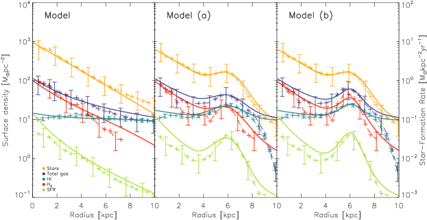
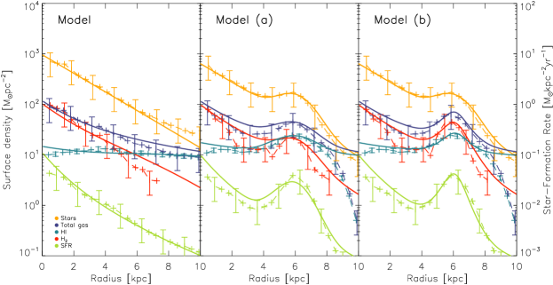
Figure 20: Radial profiles derived from observations (dashed lines) and from the analytical model (solid lines). The models correspond to model 1, 2, and 3. The models are presented in Table 3. The $\rm{H_{2}}$ profiles are limited by the detection threshold of 3 $\sigma$ within three velocity channels, corresponding to 2.8 $\rm{M_{\odot}pc^{-2}}$.

10.2 The dynamical model

The dynamical model is based on the N-body sticky particle code described in Vollmer et al. (2001). The particles are separated in two distinct phases: a non-collisional phase that reproduces the dark matter and stellar component of NGC 4654 and a collisional component for the ISM. The model takes into account both the gravitational interaction with the neighboring galaxy NGC 4369 and the influence of ram pressure stripping over $1$ Gyr. The ram pressure time profile is of Lorentzian form, which is consistent with highly eccentric orbits of galaxies within the Virgo cluster (Vollmer et al. 2001). The effect of ram pressure stripping is simulated by an additional pressure on the clouds in the wind direction, defined as $p_{\rm{ram}}=\rho v_{\rm{turb}}^{2}\sim$ 200 cm${}^{-3}\rm km\ s^{-1}$. Only clouds that are not shielded by other clouds are affected by ram pressure. The star-formation is assumed to be proportional to the cloud collision rate. Stars are formed by cloud-cloud collision and added to the total number of particles as zero-mass points with the position and the velocity of the colliding clouds. The information about the time of creation is attached to each new star particle, making it possible to model the $\rm{H\alpha}$ emission for each snapshot using stars created less than 10 Myr ago. The UV emission is modeled by the UV flux from single stellar population models from STARBURST99 (Leitherer et al. 1999). The total UV flux corresponds to the extinction-free distribution of the UV emission from newly created star particles. The cloud masses range between 3 $\times$ 10⁵ and 3 $\times$ 10⁶ $\rm{M_{\odot}}$. The atomic and molecular phases of the ISM are separated by computing the molecular fraction $f_{\rm{mol}}$ using (Eq. 30 and Eq. 31). Observational input parameters are presented in Table 1. The dynamical model produces CO, $\rm{H\textsc{i}}$, FUV, stellar mass and $\rm{H\alpha}$ data cubes at the spectral and spatial resolution of the observations. This first set of modeled data is used to produce derived quantities such as total mid-plane pressure, SFR, star-formation efficiency and Toomre $Q$ criterion in order to carry out a complete comparative study between the model and the observations.

Contrary to the analytical model, the dynamical model gives direct access to two quantities that are difficult to observe although fundamental: the volume density $\rho$ of the gas and its intrinsic 3D velocity dispersion $v_{\rm{disp}}$. The model neglects supernova feedback, which may be the origin of an increased gas velocity dispersion and an enhancement of the SFR within dense gas regions.

Three different versions of the model were produced: (i) constant pressure of $p=$ 200 cm^-3$\rm km\ s^{-1}$; (ii) constant ram pressure of $p=$ 100 cm^-3$\rm km\ s^{-1}$; (iii) no ram pressure. Only the model with a strong ram pressure wind was able to reproduce both the extended HI gas tail and the $\rm{high\ H\textsc{i}\ surface\ density\ region}$, so we chose to focus our study on this version. The maps obtained from the other versions are presented in Appendix G. We search by eye for the relevant timestep that reproduces the available observations best. A summary table of the comparison between the model and observations is presented in Table 4.

10.2.1 Stellar and atomic gas surface densities

Maps of the surface density of atomic gas and stars are shown in Fig. 21. The stellar distribution of the dynamical model is highly asymmetric. The diffuse stellar disk extends 9 kpc to the southeast compared to 12 kpc to the northwest. Toward the northwest an overdense stellar arm is formed. At the end of this stellar arm, a region of high $\rm{H\textsc{i}}$ surface density appears in the model, with total gas surface densities on the order of 50 $\rm{M_{\odot}pc^{-2}}$. Beyond the southeastern edge of the optical disk an extended $\rm{H\textsc{i}}$ gas tail is formed with surface densities of 5-10 $\rm{M_{\odot}pc^{-2}}$. Another high $\rm{H\textsc{i}}$ surface density region is observed south of the galaxy center with $\rm{\Sigma_{\rm{HI}}}$ ¿ 40 $\rm{M_{\odot}pc^{-2}}$. By studying previous timesteps of the model, we identified this region as an overdensity with a lifetime of few tens million years created accidentally at this position. We do not consider this overdensity as relevant for analysis.

Qualitatively, the overall model stellar and gaseous distributions are consistent with observations (Fig. 1). The overdense stellar arm is well reproduced, with a comparable $\rm{high\ H\textsc{i}\ surface\ density\ region}$ at its end. The $\rm{H\textsc{i}}$ gas tail in the southeast direction is also well reproduced by the dynamical model. However, the northwestern half of the diffuse stellar disk is much more extended in the model than in the observations. Quantitatively, the stellar arm presents similar surface densities, with $\Sigma_{\star}=200-500$ $\rm{M_{\odot}pc^{-2}}$. The model $\rm{high\ H\textsc{i}\ surface\ density\ region}$ presents comparable $\rm{H\textsc{i}}$ surface densities, with a maximum of $\rm{\Sigma_{\rm{HI}}}$ $\sim$ 50 $\rm{M_{\odot}pc^{-2}}$ compared to the observed maximum of 35 $\rm{M_{\odot}pc^{-2}}$. However, the $\rm{H\textsc{i}}$ surface density in the southeastern gas tail is 2 to 3 times higher than in the observations.

The dynamical model is therefore able to reproduce the dense stellar arm, the $\rm{high\ H\textsc{i}\ surface\ density\ region}$ in the northwest and the $\rm{H\textsc{i}}$ tail. However, it overestimates the influence of the ram pressure stripping and does not reproduce properly the diffuse stellar component.

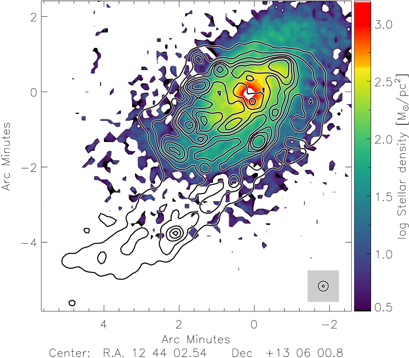
Figure 21: NGC 4654 dynamical model. The colors correspond to the stellar surface density. The contours correspond to the $\rm{H\textsc{i}}$ surface density. Contour levels are 1, 5, 10, 15, 20, and 30 $\rm{M_{\odot}pc^{-2}}$. The model data are convolved to the same spatial resolutions as the observations.

10.2.2 Molecular and total gas surface densities

The molecular gas map of the model is presented in Fig. 22. Its maximum is reached in the galaxy center with $\rm{\Sigma_{\rm{H_{2}}}}$ = 170 $\rm{M_{\odot}pc^{-2}}$. The model forms an overdense arm in the northwest direction with $\rm{\Sigma_{\rm{H_{2}}}}$ $\sim$ 40 $\rm{M_{\odot}pc^{-2}}$  which follows the stellar arm. On the opposite side, a southeastern spiral arm with lower surface densities is present. Moreover, an external gas arm is created without any correlation with the stellar distribution in the southern edge of the disk. This gas arm is identified as a consequence of shear motions induced by the combined effect of galaxy rotation and ram pressure stripping.

As for the $\rm{H\textsc{i}}$ gas, the general distribution of $\rm{H_{2}}$ gas is broadly consistent with observations (Fig. 12). The average surface density within the northwestern arm is almost equivalent to the observations. The local maximum within the $\rm{high\ H\textsc{i}\ surface\ density\ region}$ is about 40 $\rm{M_{\odot}pc^{-2}}$, which is almost two times lower than the observed value with a modified $\rm{\alpha_{\rm{CO}}}$ and equivalent to observations with a constant conversion factor, $\rm{\alpha_{\rm{CO}}^{\rm{MW}}}$. The galaxy center also presents comparable surface density as observations. The differences between the model and the observations are essentially: (i) the presence of the southeastern spiral arm that we did not intend to reproduce with the model; (ii) the overdense external gas arm formed in southern edge of the galactic disk, suggesting that the model slightly overestimates the strength of the ram pressure stripping.

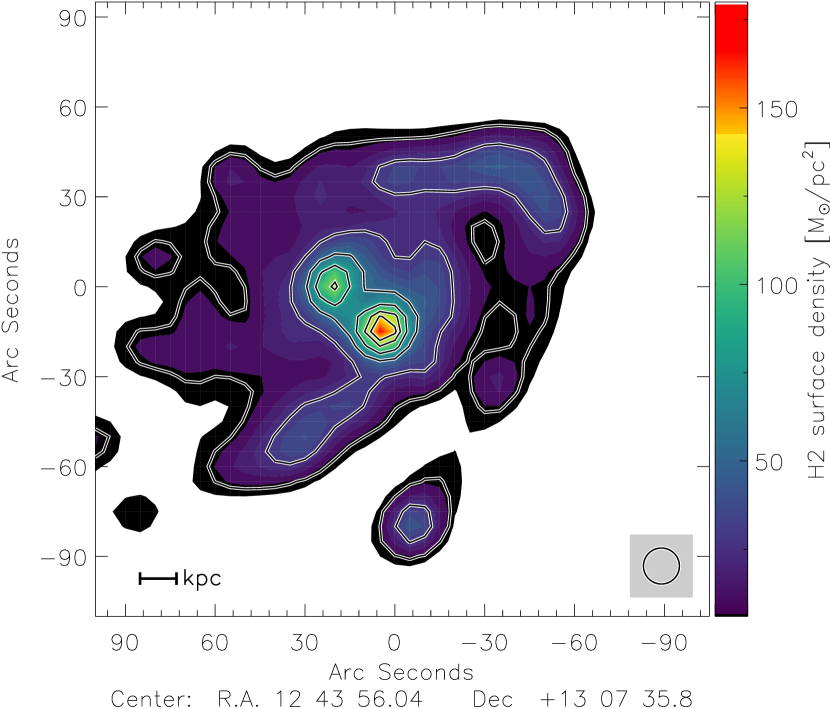
Figure 22: Molecular gas surface density of NGC 4654 from the dynamical model. Contour levels are 2, 5, 10, 30, 60, 90, and 120 $\rm{M_{\odot}pc^{-2}}$.

We added the atomic gas to the molecular gas to study the distribution of the total gas of the model (Fig. 23). Since on one hand the molecular gas surface density is consistent with observations with a constant conversion factor but on the other hand the $\rm{H\textsc{i}}$ is slightly overestimated, the total gas map of the model provides an intermediate solution between observations with $\rm{\alpha_{\rm{CO}}^{\rm{MW}}}$ and a modified $\rm{\alpha_{\rm{CO}}}$. The maximum of $\Sigma_{\rm gas}$ reached in the $\rm{high\ H\textsc{i}\ surface\ density\ region}$ is 90 $\rm{M_{\odot}pc^{-2}}$, which is 10 $\rm{M_{\odot}pc^{-2}}$ above the observations with a constant conversion factor and 30 $\rm{M_{\odot}pc^{-2}}$ below the observations with a modified conversion factor. To conclude, the model seems to be able to reproduce quite accurately the general distribution of the total gas of NGC 4654. It is, however, slightly more similar to observations with a constant factor than with a modified factor $\rm{\alpha_{\rm{CO}}}$.

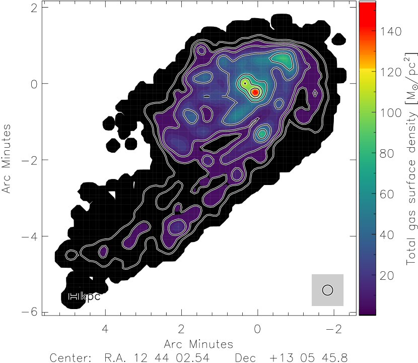
Figure 23: Total gas surface density of NGC 4654 from the dynamical model. Contour levels are 2, 5, 10, 30, 60, 90 and 120 $\rm{M_{\odot}pc^{-2}}$

10.2.3 Star-formation rate

To compute the model SFR, we used the FUV map generated by the dynamical model normalized to the total observed SFR. The model SFR map is presented in Fig. 24. The maximum of the SFR is reached in the galaxy center with $\rm{\dot{\Sigma}_{\star}}$ = 0.2 M_⊙kpc^-2yr^-1. Toward the northwest, a higher SFR surface density arm is observed, corresponding to the dense stellar and molecular gas surface density arm. We also note the presence of a slightly enhanced $\rm{\dot{\Sigma}_{\star}}$ arm following the southeastern spiral arm on the opposite side of the galaxy.

The general morphology of the SFR in the model is consistent with observations, except for the higher SFR arm along the southeast spiral arm, which is not observed (Fig. 7). This could be however linked to the small enhancement of the $\rm{H\alpha}$ emission observed in Fig. 2. The maximum of the SFR is reached in the galaxy center, contrary to observations where the maximum is located in the $\rm{high\ H\textsc{i}\ surface\ density\ region}$. The model SFR is 2-3 times lower in the northwestern region and 2-3 times higher in the galaxy center than the corresponding observed SFRs.

To conclude, the model seems to be able to reproduce qualitatively the SFR distribution of NGC 4654 but not quantitatively. As mentioned in the introduction of this section, we can presume that this is due to the absence of supernova feedback in the model.

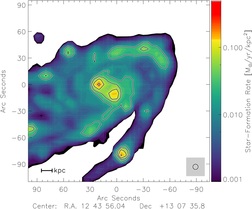
Figure 24: Star-formation rate of NGC 4654 from the dynamical model. Contours levels correspond to 0.02, 0.05, 0.10 and 0.20 $\rm{M_{\odot}}$kpc^-2yr^-1.

10.2.4 $R_{\rm{mol}}$-$P_{\rm{tot}}$ and $\rm{\Sigma_{\rm{H_{2}}}}$-$\rm{\dot{\Sigma}_{\star}}$ correlations

The model correlation between the molecular fraction of the ISM and the total gas pressure is presented in Fig. 25. The $R_{\rm{mol}}$-$P_{\rm{tot}}$ slope is 0.65 $\pm$ 0.19, which is significantly flatter than the predictions of Blitz & Rosolowsky (2006). The slope is consistent within the errors bars with the results of Leroy et al. 2008 ($0.73$), measured for local spiral galaxies of the THINGS survey. As for the observations, the model molecular fraction within the $\rm{high\ H\textsc{i}\ surface\ density\ region}$ deviates by 1 to 2 $\sigma$ from the overall correlation.

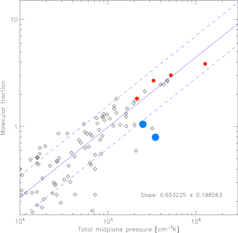
Figure 25: Molecular fraction $R_{\rm{mol}}$ as a function of the ISM pressure $P_{\rm{tot}}$ of NGC 4654 from the dynamical model. Blue points correspond to the high $\rm{H\textsc{I}}$ surface density region. Red points correspond to the galaxy center. The dashed lines correspond to $\pm$ 1 $\sigma$.

The slope of the model $\rm{\Sigma_{\rm{H_{2}}}}$-$\rm{\dot{\Sigma}_{\star}}$ relation is 0.94 $\pm$ 0.25, which is consistent within the error bars with the results of Bigiel et al. (2008) and the observed relation (Fig. 26). The SFE${}_{\rm{H_{2}}}$ varies little within the model disk, with a scatter of 0.25 dex. In contrast to our observations, the $\rm{SFE_{\rm{H_{2}}}}$ of the $\rm{high\ H\textsc{i}\ surface\ density\ region}$ does not deviate from the general correlation, with all the corresponding points included in the $\pm$ 1 $\sigma$ error bars.

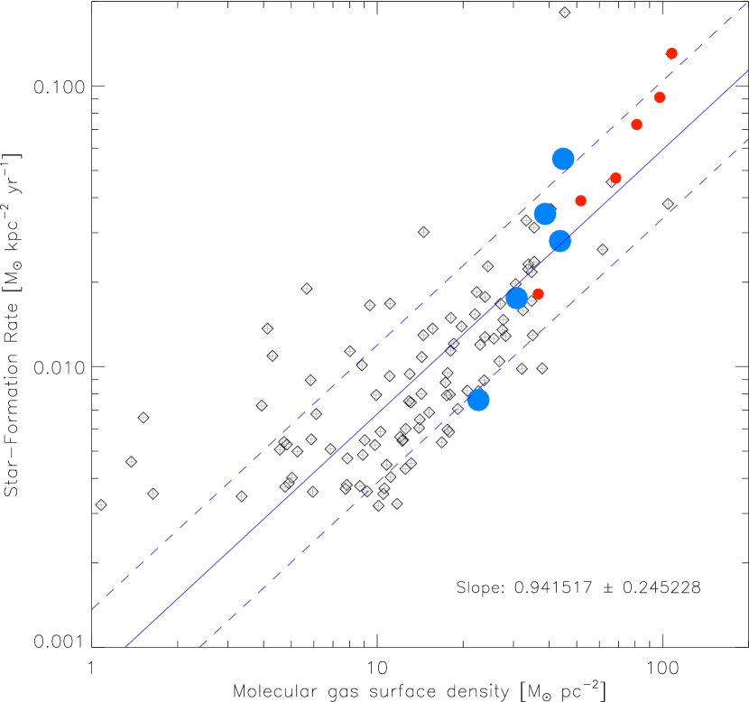
Figure 26: Star-formation Rate $\rm{\dot{\Sigma}_{\star}}$ as a function of molecular gas surface density $\rm{\Sigma_{\rm{H_{2}}}}$ of NGC 4654 from the dynamical model. Blue points correspond to the high $\rm{H\textsc{I}}$ surface density region. Red points correspond to the galaxy center. The dashed lines correspond to $\pm$ 1 $\sigma$.

The study of the $R_{\rm{mol}}$-$P_{\rm{tot}}$ and the $\rm{\Sigma_{\rm{H_{2}}}}$-$\rm{\dot{\Sigma}_{\star}}$ correlations revealed that the dynamical model reproduces faithfully the decrease in $R_{\rm{mol}}/P_{\rm{tot}}$ in the $\rm{high\ H\textsc{i}\ surface\ density\ region}$. However, the model is not able to reproduce the observed enhancement of the $\rm{SFE_{\rm{H_{2}}}}$ in this region.

10.2.5 Velocity field, linewidths, and velocity dispersion

The velocity field of the dynamical model (Fig. 27) presents straight iso-contours along the major axis in the northwest direction. These results reveal a well-defined velocity gradient toward the northwest along the major axis, that is also observed. A velocity plateau is reached in the southeast side of the disk along the major axis. The iso-contours along the minor axis are curved to the southeast, which is also consistent with the observations. The velocity field in the $\rm{H\textsc{i}}$ tail increases slightly therein, while in the observations, the region is decoupled from the galaxy rotation. All these results are consistent with previous studies of Vollmer (2003).

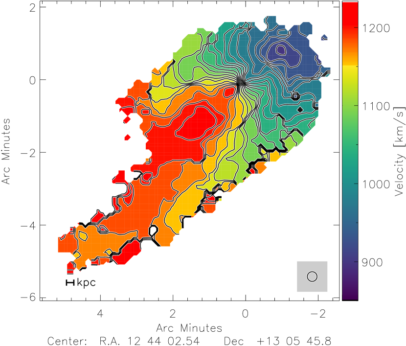
Figure 27: $\rm{H\textsc{i}}$ velocity field. Top panel: From VIVA data. Bottom panel: From the dynamical model.

As mentioned in the introduction of this section, the 3D dynamical model allows us to investigate the velocity dispersion of the ISM. An increase in the $\rm{H\textsc{i}}$ linewidth within the disk can be explained by: (i) the presence of a velocity gradient within a resolution element or (ii) an increase in the intrinsic velocity dispersion of the gas caused by local phenomena and physical conditions. In order to separate the broadening of the linewidth generated by these two scenarios, we computed two different maps: (i) the $\rm{H\textsc{i}}$ moment 2 map of the dynamical model; (ii) the 3D velocity dispersion map based on the velocity dispersion obtained for each particle using its 50 closest neighbors. The two resulting maps are presented in Fig. 28.

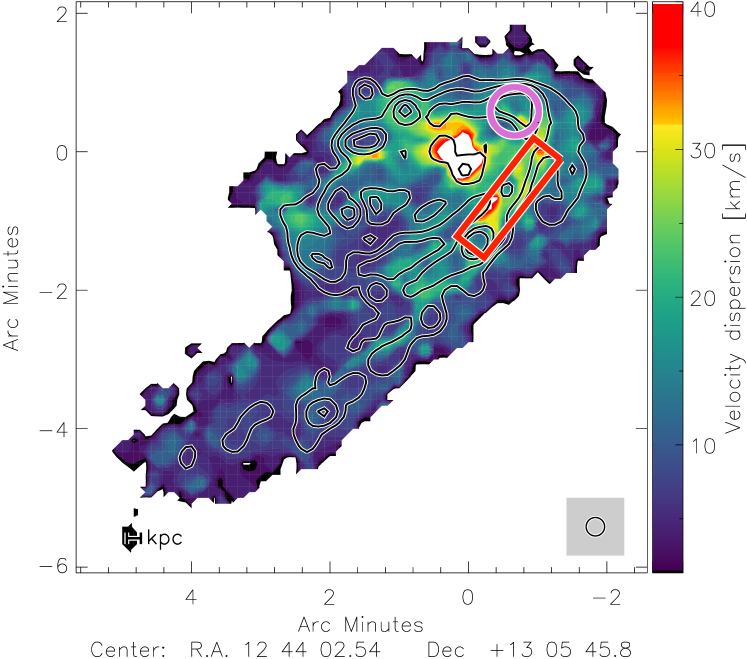
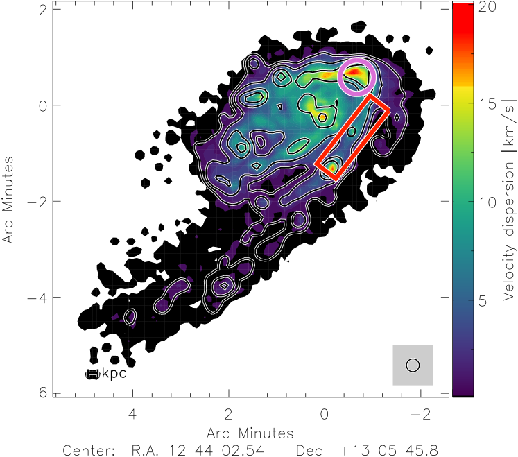
Figure 28: Gas velocity dispersion. Top panel: observed VIVA $\rm{H\textsc{i}}$ velocity dispersion (moment 2). Middle panel: velocity dispersion (moment 2) of the dynamical model. Bottom panel: intrinsic 3D velocity dispersion. The pink circle corresponds to the $\rm{high\ H\textsc{i}\ surface\ density\ region}$. The red rectangle corresponds to the external gas arm. Contours correspond to $\rm{H\textsc{i}}$ surface densities of $\rm{\Sigma_{\rm{HI}}}$ = 5, 10, 20 and 50 $\rm{M_{\odot}pc^{-2}}$.

The moment 2 map of the model reveals that the broadest velocity dispersion is created in the galaxy center with $\Delta$v $\sim$ 50 km s^-1. In the $\rm{high\ H\textsc{i}\ surface\ density\ region}$, the velocity dispersion is only 5 km s^-1 above the values at the same radius on the opposite side of the disk, with a mean $\Delta$v $\sim$ 20 km s^-1. Within the external gas arm, the velocity dispersion is broader than in the rest of the disk, with $\Delta$v = 20-40 km s^-1. This result is consistent with the assumption that the ram pressure strength in the model is too strong because the band disappears in models without any ram pressure stripping. The velocity dispersion map shows an enhancement of the dispersion within the $\rm{high\ H\textsc{i}\ surface\ density\ region}$, reaching a maximum of 18 $\rm km\ s^{-1}$. Within the external gas arm, no increase is measured. The mean velocity dispersion is $\overline{v}_{\rm disp}=5\leavevmode\nobreak\ \rm km\leavevmode\nobreak\ s^{-1}$ therein. We therefore suggest that the velocity dispersion within the northwest region is unrelated to the velocity gradient, while the rise in the external gas arm seems to be its direct outcome.

10.2.6 The model Toomre stability criterion

The Toomre stability criterion of the dynamical model is computed using Eq. 16. To compute $\kappa$, we used direct measurements of velocities and distances to the center for every mass point within the model. The velocity dispersion $v_{\rm disp}$ corresponds to the real dispersion presented in Fig. 28. A local minimum is reached in the $\rm{high\ H\textsc{i}\ surface\ density\ region}$, with $Q<0.5$ while in the rest of the disk the Toomre criterion is around $Q$ = 1. This result is consistent with observations, suggesting that even in the dynamical model, the region is unstable with respect to fragmentation.

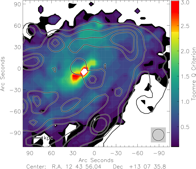
Figure 29: Toomre $Q$ parameter of NGC 4654 from the dynamical model. Contours levels are 0.5, 1 and 1.5.

10.2.7 Summary of the dynamical model

Table 4 gathers all results from the study of the dynamical model. The dynamical model appears to be closer to the observations with a constant conversion factor $\rm{\alpha_{\rm{CO}}^{\rm{MW}}}$. The model reproduces $\rm{H\textsc{i}}$ observations of NGC 4654: the $\rm{H\textsc{i}}$ tail and the $\rm{high\ H\textsc{i}\ surface\ density\ region}$ being well reproduced with quite comparable surface densities. Although the stellar arm is well reproduced by the model, the diffuse stellar disk is much more extended toward the northwest than the observations. The spatial distribution of the molecular gas matches the observations but is underestimated by a factor of 2 along the dense stellar arm. The observed enhancement of the SFR in the $\rm{high\ H\textsc{i}\ surface\ density\ region}$ is not reproduced by the model, suggesting that the inclusion of local physical phenomenon such as supernova feedback is mandatory to reproduce such high star-formation. The deviation of the $\rm{high\ H\textsc{i}\ surface\ density\ region}$ from the galaxy correlation $R_{\rm{mol}}$-$P_{\rm{tot}}$ is also present in the model. However, the model $\rm{SFE_{\rm{H_{2}}}}$ does not decrease in the $\rm{high\ H\textsc{i}\ surface\ density\ region}$ as it is observed. The Toomre stability parameter of the dynamical model decreases below one within the $\rm{high\ H\textsc{i}\ surface\ density\ region}$, suggesting that the region is unstable with respect to gas fragmentation. Excluding the formation of an external gas arm caused by an overestimation of the ram pressure stripping in the model, the reproduction of the velocity field of the dynamical model is also robust with the observations. A velocity gradient in the northwestern direction is measured with comparable strength. Separate studies of the observed velocity dispersion and the intrinsic velocity dispersion within the model suggests that the broader linewidth measured in the $\rm{high\ H\textsc{i}\ surface\ density\ region}$ are produced by a real increase in the intrinsic velocity dispersion and not by a sole consequence of the velocity gradient caused by the ram pressure stripping.

Table 4: Comparison between the observations and the dynamical model.

	Observations ( $\rm{\alpha_{\rm{CO}}^{\rm{MW}}}$ / 2$\rm{\alpha_{\rm{CO}}^{\rm{MW}}}$)	Model
Mean $\rm{\Sigma_{\rm{HI}}}$ in the gas tail	1.86 $\rm{M_{\odot}pc^{-2}}$	2.96 $\rm{M_{\odot}pc^{-2}}$
Max $\rm{\Sigma_{\rm{HI}}}$ in the $\rm{high\ H\textsc{i}\ surface\ density\ region}$	40.6 $\rm{M_{\odot}pc^{-2}}$	43.6 $\rm{M_{\odot}pc^{-2}}$
Mean $\rm{\Sigma_{\rm{H_{2}}}}$ in the northwestern dense stellar arm	30-40 $\rm{M_{\odot}pc^{-2}}$	30-40 $\rm{M_{\odot}pc^{-2}}$
Max $\rm{\Sigma_{\rm{H_{2}}}}$ in the galaxy center	173 $\rm{M_{\odot}pc^{-2}}$	170 $\rm{M_{\odot}pc^{-2}}$
Max $\rm{\Sigma_{\rm{H_{2}}}}$ in the $\rm{high\ H\textsc{i}\ surface\ density\ region}$	49.6 $\rm{M_{\odot}pc^{-2}}$ / 99.3 $\rm{M_{\odot}pc^{-2}}$	49.5 $\rm{M_{\odot}pc^{-2}}$
Max $\rm{\dot{\Sigma}_{\star}}$ in the $\rm{high\ H\textsc{i}\ surface\ density\ region}$	0.27 $\rm{M_{\odot}}$ kpc-2 yr-1	0.07 $\rm{M_{\odot}}$ kpc-2 yr-1
Slope of $\rm{\Sigma_{\rm{H_{2}}}}$-$\rm{\dot{\Sigma}_{\star}}$correlation	1.02 ($\pm$0.18)	0.94 ($\pm$0.25)
$\rm{high\ H\textsc{i}\ surface\ density\ region}$ deviation from the correlation	0.1-0.2 dex	-
Slope of $R_{\rm{mol}}$-$\rm{P_{\rm{tot}}}$ correlation	1.00 ($\pm$0.18)	0.65 ($\pm$0.20)
$\rm{high\ H\textsc{i}\ surface\ density\ region}$ deviation from the correlation	0.2-0.3 dex	0.2 dex

11 Discussion

In this section we investigate which kind of physical environment is required to maintain the $\rm{high\ H\textsc{i}\ surface\ density\ region}$ in its current state. We first compare the region of NGC 4654 with a similar region of enhanced Hi surface density in another Virgo galaxy, NGC 4501. Then, we carry out a comparative study between the analytical and dynamical models to highlight what these regions have in common and what distinguishes them. Finally, we conclude the discussion on the suggested youth of the northwestern region.

11.1 Comparison with NGC 4501

NGC 4501 is another Virgo galaxy studied in detail in Nehlig et al. (2016) that is undergoing active ram pressure stripping. The interaction is nearly edge-on, leading to a well-defined compression front on the western side of the disk. NGC 4501 also presents a region where the $\rm{H\textsc{i}}$ surface density is particularly high, located in this compressed front. Nehlig et al. (2016) studied the variation of the $R_{\rm{mol}}/P_{\rm{tot}}$ and $\rm{SFE_{\rm{H_{2}}}}$ correlations within the galaxy. They showed that the $\rm{high\ H\textsc{i}\ surface\ density\ region}$ of NGC 4501 presents: (i) an excess in the $\rm{H\textsc{i}}$ surface density up to 27 $\rm{M_{\odot}pc^{-2}}$; (ii) a slight increase in the $\rm{SFE_{\rm{H_{2}}}}$ of 0.1 dex; (iii) a significant decrease in $R_{\rm{mol}}/P_{\rm{tot}}$ of 0.3-0.4 dex; (iv) a drop of the Toomre $Q$ parameter close to the value of 1; (v) an increase in the $P_{\rm gas}/P_{\star}$ ratio up to 0.7. In the following, the properties of the $\rm{high\ H\textsc{i}\ surface\ density\ region}$ of NGC 4654 and NGC 4501 are compared in detail.

The $\rm{high\ H\textsc{i}\ surface\ density\ region}$ of NGC 4654 also exceeds the usual $10$-$15$ $\rm{M_{\odot}pc^{-2}}$ observed in spiral galaxies (Leroy et al. 2008), with an even higher maximum $\rm{\Sigma_{\rm{HI}}}$ = 40 $\rm{M_{\odot}pc^{-2}}$. The slight increase in the star-formation efficiency of NGC 4501 is comparable with the one obtained with a modified conversion factor for the $\rm{high\ H\textsc{i}\ surface\ density\ region}$ of NGC 4654, namely 0.1 dex above the $\rm{\Sigma_{\rm{H_{2}}}}$-$\rm{\dot{\Sigma}_{\star}}$ correlation. Whereas the metallicity profile of NGC 4654 observed by Skillman et al. (1996) and corrected following Curti et al. (2020) suggests an increase in the conversion factor within the $\rm{high\ H\textsc{i}\ surface\ density\ region}$, this is not the case for NGC 4501. The overall metallicity profile of NGC 4501 is significantly higher and flatter than the profile of NGC 4654. At the outer radii the metallicity of NGC 4501 also measured by Skillman et al. (1996) is about twice as high as that of NGC 4654. The metallicity within the $\rm{high\ H\textsc{i}\ surface\ density\ region}$ of NGC 4501 remains therefore higher than solar. This suggests that the conversion factor within the $\rm{high\ H\textsc{i}\ surface\ density\ region}$ of NGC 4501 is close to the Galactic value while for NGC 4654 a two times higher conversion factor seems appropriate. With such an increased conversion factor, the star-formation efficiencies with respect to the molecular gas of NGC 4654 and NGC 4501 are well comparable. This result supports the assumption of an increased $\rm{\alpha_{\rm{CO}}}$ in the $\rm{high\ H\textsc{i}\ surface\ density\ region}$. As for NGC 4501, a significant drop of the $R_{\rm mol}/P_{\rm tot}$ of 0.2-0.3 dex is observed within the $\rm{high\ H\textsc{i}\ surface\ density\ region}$ of NGC 4654. The Toomre $Q$ parameter in the northwestern region of NGC 4654 is half than that estimated by Nehlig et al. (2016) in the $\rm{high\ H\textsc{i}\ surface\ density\ region}$ of NGC 4501, with a minimum of $Q\sim 0.5$. The total gas surface density of NGC 4501 in the $\rm{high\ H\textsc{i}\ surface\ density\ region}$ is approximately $\Sigma_{\rm gas}=40-50$ $\rm{M_{\odot}pc^{-2}}$, while for NGC 4654, with a modified conversion factor, the total surface density reaches a local maximum around $\Sigma_{\rm gas}$ = 90 $\rm{M_{\odot}pc^{-2}}$. This difference may explain partially the lower Toomre $Q$ parameter found in NGC 4654. We produced a map of the observed ratio between the gas pressure and the pressure term due to the stellar gravitational potential $P_{\rm gas}/P_{\star}$ (Fig. 30). The map shows that the gas in the $\rm{high\ H\textsc{i}\ surface\ density\ region}$ is self-gravitating with $P_{\rm gas}/P_{\star}=1.7$ at its maximum. This value is 2.5 times higher than that of the $\rm{high\ H\textsc{i}\ surface\ density\ region}$ of NGC 4501. While in NGC 4501 the ISM in the $\rm{high\ H\textsc{i}\ surface\ density\ region}$ is approaching self-gravitation, the total mid-plane pressure of NGC 4654 in the corresponding region is dominated by $P_{\rm gas}$. The difference between the two $\rm{high\ H\textsc{i}\ surface\ density\ region}$ of NGC 4501 and NGC 4654 might be also explained by the higher total gas surface density of NGC 4654 compared to that of NGC 4501.

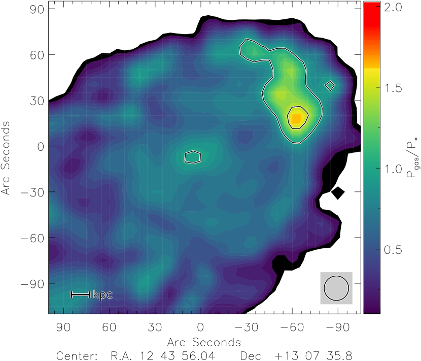
Figure 30: NGC 4654 observed mid-plane pressure counterparts ratio $P_{\rm gas}$/$P_{\star}$. Contour levels correspond to 1 and 1.5.

Since the two regions are comparable in all stated points, the $\rm{high\ H\textsc{i}\ surface\ density\ region}$ of NGC 4654 being an enhanced version of that of NGC 4501, it can be assumed that the underlying physical processes are the same: a high gas surface density together with a somewhat increased velocity dispersion and a low Toomre $Q$ parameter. Whereas we know that NGC 4654 undergoes both gravitational interaction and ram pressure stripping, NGC 4501 experiences only ram pressure stripping (Vollmer et al. 2008). Therefore, we conclude that the combined effect of ram pressure stripping and gravitational interaction gave rise to a higher gas surface density in the compressed region of NGC 4654. On the other hand, the reaction of the ISM including star-formation is the same in the two galaxies. We speculate that the $\rm{high\ H\textsc{i}\ surface\ density\ region}$s in the gravitationally interacting galaxy NGC 2207 (Elmegreen et al. 2016) are in the same physical state.

11.2 The radio spectral index

Vollmer et al. (2010) studied the radio spectral index $\upvarepsilon$ between $6$ and $20$ cm of 8 Virgo galaxies affected by ram pressure stripping. The spectral index along the northwestern stellar arm is significantly steeper than that of the rest of the disk ($\upvarepsilon\ga-0.8$). The spectral index reaches its maximum in the $\rm{high\ H\textsc{i}\ surface\ density\ region}$, with $\upvarepsilon\sim-0.5$, i.e, it is close to the typical value for a population of cosmic ray electrons at the time of injection. This suggests that the star-forming region is relatively young, only a few 10 Myr old (Beck 2015).

11.3 Joining between the analytical and dynamical models

In both, the analytical or dynamical model, an increase in the velocity dispersion combined with a decrease in the Toomre $Q$ parameter are mandatory to reproduce the observations. Although the velocity dispersion increases consistently between these two models, the resulting SFR is significantly lower in the dynamical model than in the analytical model.

The main difference between the two models lies in the cloud density $\rho_{\rm cl}$ within the $\rm{high\ H\textsc{i}\ surface\ density\ region}$. The dynamical model does not consider cooling and heating mechanisms of the ISM through self-gravitating collapse and stellar feedback. This means that the model does not allow clumping in regions that are presumed to be dense, leading to an underestimation of the local SFR. In the analytical and dynamical models, the decrease in the Toomre $Q$ parameter induces an increase in the global density. Whereas the volume filling factor is assumed to be constant in the dynamical model, it shows an increase by about a factor of two in the dynamical model leading to an increase in the SFR (Eq. 23). Despite the fact that the large-scale density distributions are consistent between the two models, the small-scale gas density and SFR are poorly reproduced by the dynamical model. In the latter, the star-formation is purely driven by collisions between gas particles, while in the analytical model supernova feedback determines the ISM properties at small-scales which have a significant impact on star-formation.

11.4 Reaching atomic gas surface densities in excess of 30 $M_{\odot}pc^{-2}$ in galaxies with and without stellar feedback

Using the analytical model, we investigated how high $\rm{H\textsc{i}}$ surface density regions with $\rm{\Sigma_{\rm{HI}}}$ ¿ 30 $\rm{M_{\odot}pc^{-2}}$ can be created and maintained. The question is therefore to understand how far should the velocity dispersion be increased to reach such surface densities without any decrease in the Toomre $Q$ parameter or, conversely, how much must the Toomre $Q$ parameter be decreased below the critical value of one to reach such surface densities without increasing the velocity dispersion.

We first modeled an unperturbed disk with $\delta=5$, a mean Toomre $Q$ parameter of $Q=1.5$ and an accretion rate of $\dot{M}\leavevmode\nobreak\ =\leavevmode\nobreak\ 0.1\leavevmode\nobreak\ \rm{M_{\odot}yr^{-1}}$. The additional free parameters $\xi$, $v_{\rm disp}^{\star}$ and $\gamma$ were not modified. We then created a $\rm{high\ H\textsc{i}\ surface\ density\ region}$ with $\Sigma_{\rm HI}\sim 30$ $\rm{M_{\odot}pc^{-2}}$ at a radius of 6 kpc by varying the gas density via the Toomre Q parameter or the velocity dispersion via the mass accretion rate. In both cases the stellar feedback is strongly increased. We found that: (i) To obtain a $\rm{high\ H\textsc{i}\ surface\ density\ region}$ without an increase in the velocity dispersion, the Toomre $Q$ parameter must be $Q\leq 0.3$. The resulting SFR in this region is about 60% of the SFR in the galaxy center. The molecular gas surface density reaches high values, leading to a molecular fraction of $R_{\rm{mol}}$ $\sim$ 2 in this region ; (ii) To obtain a $\rm{high\ H\textsc{i}\ surface\ density\ region}$ without a decrease in the Toomre $Q$ parameter, the increase in the velocity dispersion in this region must be $\Delta v_{\rm disp}$ $\geq$ 16 $\rm km\ s^{-1}$. The resulting SFR in this region is about 40% of the SFR in the galaxy center. The molecular fraction is only $R_{\rm{mol}}$ $\sim$ 0.5 in this region.

The analytical model therefore suggests that it is theoretically possible to reach $\rm{\Sigma_{\rm{HI}}}$ ¿ 30 $\rm{M_{\odot}pc^{-2}}$ by modifying only the Toomre $Q$ parameter or the velocity dispersion. We found that the star-formation rate does not allow us to discriminate between these two extreme hypotheses. However, the resulting molecular gas surface density of the two assumptions are strongly different. This suggests that CO observations are necessary to determine if stellar feedback can keep the density of the compressed ISM approximately constant or if the density increases during a compression phase, i.e, if the velocity dispersion is abnormally high or if the Toomre $Q$ parameter is particularly low.

For the determination of the molecular fraction a CO-to-H₂ conversion factor has to be applied. In the case of a strong decrease in the Toomre $Q$ parameter a significant increase in the molecular fraction can still be observed even when a Galactic conversion factor is assumed. We conclude that, in the absence of a reliable estimate of the intrinsic velocity dispersion, it is possible to roughly estimate the influence of stellar feedback in a $\rm{high\ H\textsc{i}\ surface\ density\ region}$ located in the outer galactic disk, i.e, the balance between the decrease in the Toomre $Q$ parameter and the increase in the velocity dispersion by estimating the molecular fraction assuming a Galactic CO-to-H₂ conversion factor.

12 Conclusions

New IRAM 30m HERA CO(2-1) data were combined with VIVA $\rm{H\textsc{i}}$ data to investigate the distribution of the total gas within the disk of the Virgo spiral galaxy NGC 4654 and its ability to form stars. NGC 4654 undergoes both, a gravitational interaction with another massive galaxy and nearly edge-on ram pressure stripping. The combined effects of these interactions lead to the formation of an overdense stellar and molecular gas arm toward the northwest, ending with an abnormally high $\rm{H\textsc{i}}$ surface density region. Previous studies (Chung & Kim 2014) showed that within this region the $\rm{SFE_{\rm{H_{2}}}}$ is unusually high and the ratio of the molecular fraction to the total mid-plane pressure is significantly lower than that of the rest of the disk. With deeper CO observations of higher spatial resolution (12”) and a star-formation map based on GALEX FUV and SPITZER 24 $\rm{\mu m}$ data, we pursued this study to understand the physical properties of the ISM in the $\rm{high\ H\textsc{i}\ surface\ density\ region}$ and their impact on the ability of the ISM to form stars.

We applied two methods to determine the value of the CO-to-H₂ conversion factor within the disk of NGC 4654. Following Sandstrom et al. (2013), the first method consists in the simultaneous determination of the DGR and the conversion factor using Herschel 250$\rm{\mu m}$ FIR data as a tracer for total gas surface density. The second method is based on the determination of the DGR from direct metallicity measurements of Skillman et al. (1996) corrected according to the calibration of Curti et al. (2020). Different results were found by the two models: a constant conversion factor and an increased conversion factor by a factor of two in the $\rm{high\ H\textsc{i}\ surface\ density\ region}$. The comparison of the metallicity and the SFE of the $\rm{high\ H\textsc{i}\ surface\ density\ region}$ in NGC 4654 and NGC 4501, which has similar physical characteristics, supports the assumption of a modified conversion factor for NGC 4654 (see Sect. 11.1).

The radial profiles of the atomic gas, molecular gas and star-formation were compared to an analytical model of a star-forming turbulent clumpy disk (see Sect. 10.1). We simultaneously varied six free parameters to reproduce the available observations via two successive reduced-$\upchi^{2}$ minimizations. The radial profiles of the unperturbed southeastern and perturbed northwestern disk halves were fitted separately (see Sect. 10.1.1). Degeneracies between the free parameters were revealed, making it impossible to discriminate between the two assumptions on the CO-to-H₂ conversion factor (see Sect. 10.1.2). However, regardless of the choice of the conversion factor used to compute the molecular gas surface density, the $\rm{high\ H\textsc{i}\ surface\ density\ region}$ presents (i) an increase in the intrinsic velocity dispersion by $\sim 5$ km s^-1 (2-10 km s^-1) and (ii) a decrease in the Toomre $Q$ parameter (Fig. 19). For $\Delta v_{\rm disp}$ $\leq$ 6 km s^-1, the Toomre Q parameters drops below unity, suggesting that the region is marginally unstable with respect to gas fragmentation. The increase in velocity dispersion is compatible with the VIVA $\rm{H\textsc{i}}$ observations.

The available observations were compared to a dynamical model that takes into account the gravitational interaction and ram pressure stripping (see Sect. 10.2). The model atomic and molecular gas surface densities, velocity field, moment 2 map, slopes of the $R_{\rm{mol}}$-$P_{\rm{tot}}$ and $\rm{\Sigma_{\rm{H_{2}}}}$-$\rm{\dot{\Sigma}_{\star}}$correlations, and deviation of the $\rm{high\ H\textsc{i}\ surface\ density\ region}$ from the $R_{\rm{mol}}$-$P_{\rm{tot}}$ correlation are consistent with observations. However, the model is not able to reproduce the SFR in the $\rm{high\ H\textsc{i}\ surface\ density\ region}$ because of the absence of physical processes such as gas cooling and stellar feedback preventing the formation of small-scale clumpy regions with high volume densities.

Using the analytical model, we examined the physical conditions required to maintain a $\rm{high\ H\textsc{i}\ surface\ density\ region}$ with $\rm{\Sigma_{\rm{HI}}}$ ¿ 30 $\rm{M_{\odot}pc^{-2}}$ in the outer parts of galactic disks (see Sect. 11.4). We found that it is possible to create such a peculiar Hi region by either strongly decreasing the Toomre $Q$ parameter or by strongly increasing the velocity dispersion. The CO surface brightness is a good criterion to discriminate between these two extreme solutions. The most realistic result, however, remains a combination of the two solutions, as observed in NGC 4654.

Based on our results we suggest the following scenario for the $\rm{high\ H\textsc{i}\ surface\ density\ region}$: during a period of gas compression through external interactions the gas surface density is enhanced leading to an increased SFR and stellar feedback. Our observations and subsequent modeling suggest that under the influence of stellar feedback the turbulent velocity dispersion significantly increases and hence the increase in the gas density is only moderate (less than a factor of two). Thus, stellar feedback acts as a regulator of star-formation (see Ostriker et al. 2010, Ostriker & Shetty 2011).

Appendix A CO(2-1) rms map

Appendix B DGR minimization method - Other regions

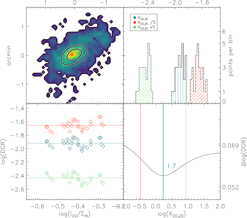
Figure 32: Same description as Fig. 9.

Figure 33: Same description as Fig. 9.

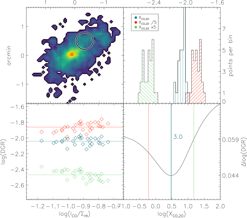
Figure 34: Same description as Fig. 9.

Appendix C Comparison between different metallicity estimation methods

Figure 35: Same description as Fig. 10. The green, red, and blue lines correspond, respectively, to the metallicity obtained from the analytical models (1), (1a), and (1b) using the molecule formation timescale with the closed box model.

Appendix D Results with a constant CO-to-H₂ conversion factor

In this section, we reproduce the same maps as in the Results sections. in order to compare the results using a constant CO-to-H₂ conversion factor $\rm{\alpha_{\rm{CO}}}$ = 4.36 $\rm{M_{\odot}(K\ \rm km\ s^{-1}\ pc^{2})^{-1}}$.

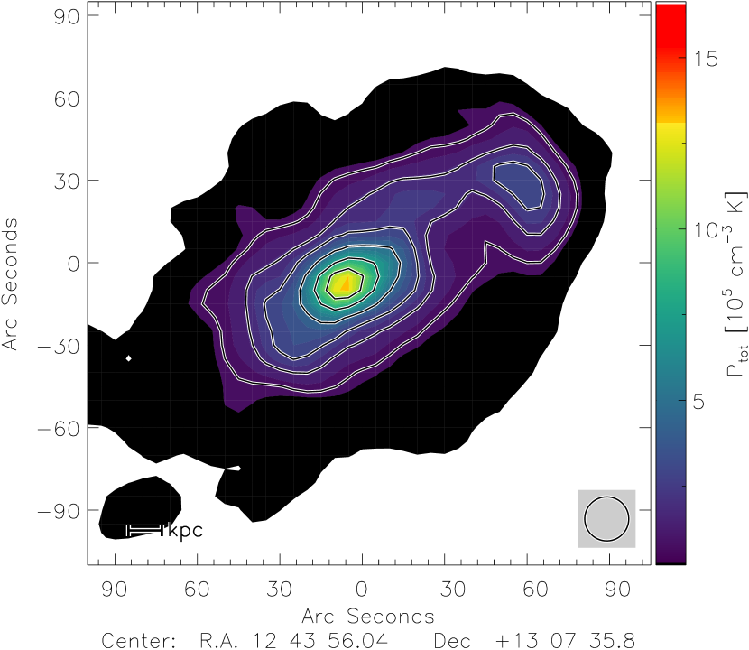
Figure 37: Total ISM mid-plane pressure. Contours levels are 1, 2, 3, 5, 8, and 11 $\times$ 10⁵ cm^-3 K. The resolution is 16”.

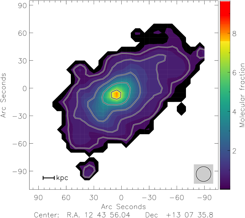
Figure 38: Molecular fraction R_mol = $\Sigma_{\rm{H_{2}}}$ / $\Sigma_{\rm{HI}}$. Contours levels are 5, 10, 30, 60, 90, 120, and 140 $M_{\odot}pc^{-2}$. The resolution is 16”.

Appendix E Toomre $Q$ criterion alternative map

Figure 39: Toomre $Q$ parameter map obtained from the observational rotation curve. Contour levels correspond to 0.5, 1, and 1.5.

Appendix F Star-formation rate comparison

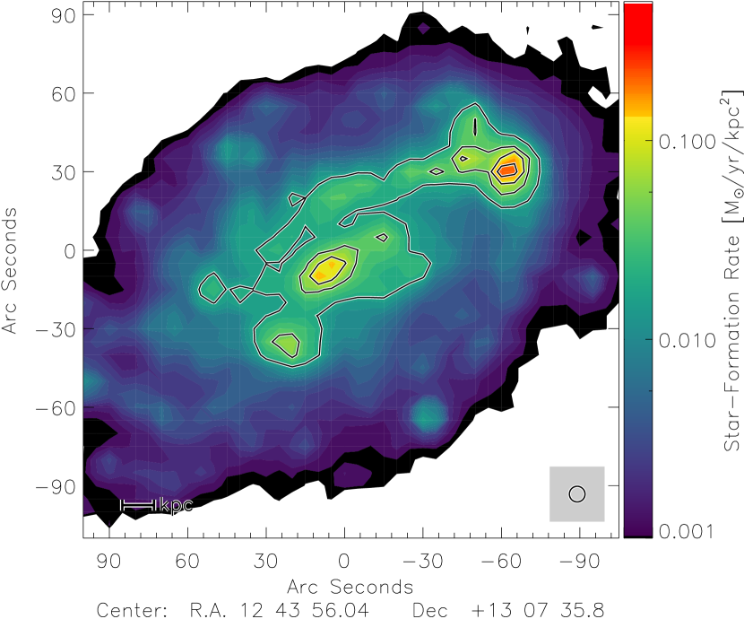
Figure 40: Star-formation map computed using $24$ $\mu$m and H$\alpha$ data.

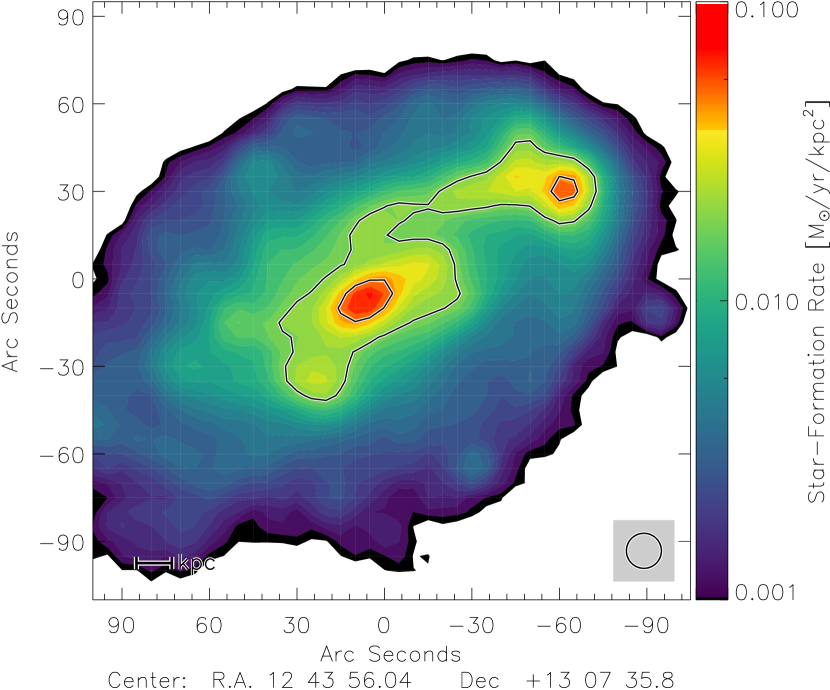
Figure 41: Star-formation map computed using FUV and TIR data.

Appendix G Alternative ram pressure stripping models

Figure 42: Half wind ram pressure model: stellar and atomic gas surface densities.

Figure 43: No wind ram pressure model: stellar and atomic gas surface density.

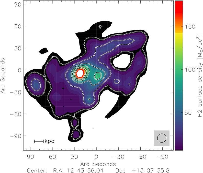
Figure 44: Half wind ram pressure model: molecular gas surface density.

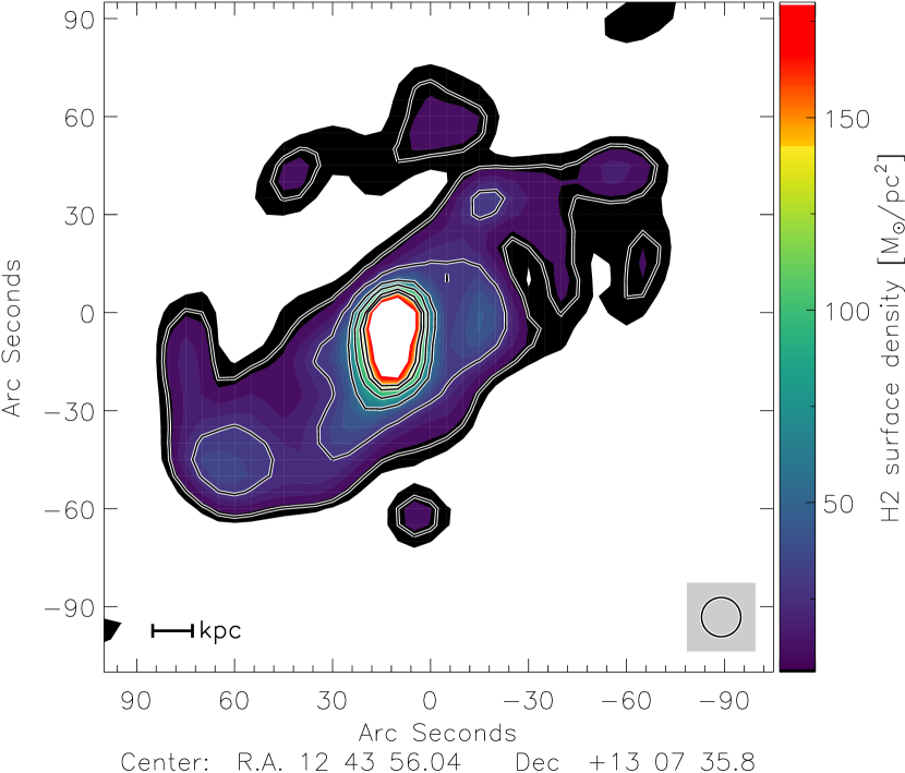
Figure 45: No wind ram pressure model: molecular gas surface density.

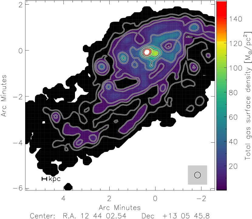
Figure 46: Half wind ram pressure model: total gas surface density.

Figure 47: No wind ram pressure model: total gas surface density.

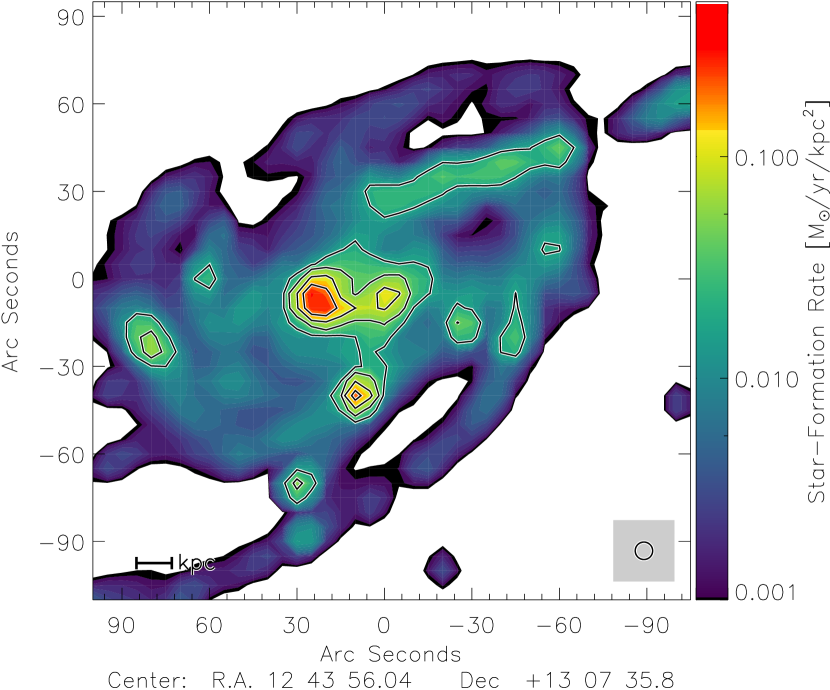
Figure 48: Half wind ram pressure model: SFR.

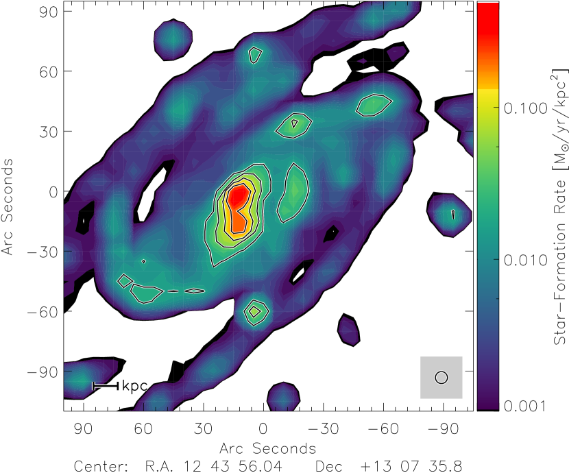
Figure 49: No wind ram pressure model: SFR.

References

- Alam et al. (2015) Alam, S., Albareti, F. D., Prieto, C. A., et al. 2015, The Astrophysical Journal Supplement Series, 219, 12
- Beck (2015) Beck, R. 2015, A&A Rev., 24, 4
- Bigiel et al. (2008) Bigiel, F., Leroy, A., Walter, F., et al. 2008, AJ, 136, 2846
- Bigiel et al. (2011) Bigiel, F., Leroy, A. K., Walter, F., et al. 2011, ApJ, 730, L13
- Blitz & Rosolowsky (2006) Blitz, L. & Rosolowsky, E. 2006, ApJ, 650, 933
- Boissier et al. (2003) Boissier, S., Prantzos, N., Boselli, A., & Gavazzi, G. 2003, MNRAS, 346, 1215
- Bolatto et al. (2013) Bolatto, A. D., Wolfire, M., & Leroy, A. K. 2013, ARA&A, 51, 207
- Bolatto et al. (2017) Bolatto, A. D., Wong, T., Utomo, D., et al. 2017, ApJ, 846, 159
- Brinchmann et al. (2004) Brinchmann, J., Charlot, S., White, S. D. M., et al. 2004, MNRAS, 351, 1151
- Chung et al. (2008) Chung, A., van Gorkom, J. H., Crowl, H., Kenney, J. D. P., & Vollmer, B. 2008, in Astronomical Society of the Pacific Conference Series, Vol. 395, Frontiers of Astrophysics: A Celebration of NRAO’s 50th Anniversary, ed. A. H. Bridle, J. J. Condon, & G. C. Hunt, 364
- Chung et al. (2007) Chung, A., van Gorkom, J. H., Kenney, J. D. P., & Vollmer, B. 2007, ApJ, 659, L115
- Chung & Kim (2014) Chung, E. J. & Kim, S. 2014, PASJ, 66, 11
- Condon et al. (1998) Condon, J. J., Cotton, W. D., Greisen, E. W., et al. 1998, AJ, 115, 1693
- Curti et al. (2017) Curti, M., Cresci, G., Mannucci, F., et al. 2017, MNRAS, 465, 1384
- Curti et al. (2020) Curti, M., Mannucci, F., Cresci, G., & Maiolino, R. 2020, MNRAS, 491, 944
- Daddi et al. (2007) Daddi, E., Dickinson, M., Morrison, G., et al. 2007, ApJ, 670, 156
- Draine et al. (2007) Draine, B. T., Dale, D. A., Bendo, G., et al. 2007, ApJ, 663, 866
- Draine & Lee (1984) Draine, B. T. & Lee, H. M. 1984, ApJ, 285, 89
- Elmegreen (1989) Elmegreen, B. G. 1989, ApJ, 338, 178
- Elmegreen et al. (2016) Elmegreen, B. G., Kaufman, M., Bournaud, F., et al. 2016, ApJ, 823, 26
- Galametz et al. (2013) Galametz, M., Kennicutt, R. C., Calzetti, D., et al. 2013, MNRAS, 431, 1956
- Gavazzi et al. (2003) Gavazzi, G., Boselli, A., Donati, A., Franzetti, P., & Scodeggio, M. 2003, A&A, 400, 451
- Genzel et al. (2010) Genzel, R., Tacconi, L. J., Gracia-Carpio, J., et al. 2010, MNRAS, 407, 2091
- Gordon et al. (2014) Gordon, K. D., Roman-Duval, J., Bot, C., et al. 2014, ApJ, 797, 85
- Gordon et al. (2017) Gordon, K. D., Roman-Duval, J., Bot, C., et al. 2017, The Astrophysical Journal, 837, 98
- Hao et al. (2011) Hao, C.-N., Kennicutt, R. C., Johnson, B. D., et al. 2011, ApJ, 741, 124
- Hasegawa (1997) Hasegawa, T. 1997, in IAU Symposium, Vol. 170, IAU Symposium, ed. W. B. Latter, S. J. E. Radford, P. R. Jewell, J. G. Mangum, & J. Bally, 39–46
- Kennicutt (1998) Kennicutt, Robert C., J. 1998, ApJ, 498, 541
- Kennicutt & Evans (2012) Kennicutt, R. C. & Evans, N. J. 2012, ARA&A, 50, 531
- Kregel et al. (2002) Kregel, M., van der Kruit, P. C., & de Grijs, R. 2002, MNRAS, 334, 646
- Leitherer et al. (1999) Leitherer, C., Schaerer, D., Goldader, J. D., et al. 1999, ApJS, 123, 3
- Leroy et al. (2011) Leroy, A. K., Bolatto, A., Gordon, K., et al. 2011, ApJ, 737, 12
- Leroy et al. (2008) Leroy, A. K., Walter, F., Brinks, E., et al. 2008, AJ, 136, 2782
- Martin et al. (2005) Martin, D. C., Fanson, J., Schiminovich, D., et al. 2005, ApJ, 619, L1
- Meixner et al. (2014) Meixner, M., Seale, J., Roman-Duval, J., Gordon, K., & HERITAGE Team. 2014, Astronomische Nachrichten, 335, 523
- Murphy et al. (2006) Murphy, E. J., Braun, R., Helou, G., et al. 2006, ApJ, 638, 157
- Nebot Gomez-Moran et al. (2020) Nebot Gomez-Moran, A., Fernique, P., & CDS Team. 2020, in Astronomical Society of the Pacific Conference Series, Vol. 522, Astronomical Data Analysis Software and Systems XXVII, ed. P. Ballester, J. Ibsen, M. Solar, & K. Shortridge, 77
- Nehlig et al. (2016) Nehlig, F., Vollmer, B., & Braine, J. 2016, A&A, 587, A108
- Noeske et al. (2007) Noeske, K. G., Weiner, B. J., Faber, S. M., et al. 2007, ApJ, 660, L43
- Ostriker et al. (2010) Ostriker, E. C., McKee, C. F., & Leroy, A. K. 2010, ApJ, 721, 975
- Ostriker & Shetty (2011) Ostriker, E. C. & Shetty, R. 2011, ApJ, 731, 41
- Pérez-Montero & Contini (2009) Pérez-Montero, E. & Contini, T. 2009, MNRAS, 398, 949
- Rahman et al. (2011) Rahman, N., Bolatto, A., & STING Collaboration. 2011, in American Astronomical Society Meeting Abstracts, Vol. 218, American Astronomical Society Meeting Abstracts #218, 130.01
- Saintonge et al. (2017) Saintonge, A., Catinella, B., Tacconi, L. J., et al. 2017, ApJS, 233, 22
- Sandstrom et al. (2013) Sandstrom, K. M., Leroy, A. K., Walter, F., et al. 2013, ApJ, 777, 5
- Schruba et al. (2011) Schruba, A., Leroy, A. K., Walter, F., et al. 2011, AJ, 142, 37
- Skillman et al. (1996) Skillman, E. D., Kennicutt, Robert C., J., Shields, G. A., & Zaritsky, D. 1996, ApJ, 462, 147
- Soida et al. (2006) Soida, M., Otmianowska-Mazur, K., Chyży, K., & Vollmer, B. 2006, A&A, 458, 727
- Tacconi et al. (2018) Tacconi, L. J., Genzel, R., Saintonge, A., et al. 2018, ApJ, 853, 179
- Tamburro et al. (2009) Tamburro, D., Rix, H. W., Leroy, A. K., et al. 2009, AJ, 137, 4424
- Tielens & Hollenbach (1985) Tielens, A. G. G. M. & Hollenbach, D. 1985, ApJ, 291, 722
- Toomre (1964) Toomre, A. 1964, ApJ, 139, 1217
- Vollmer (2003) Vollmer, B. 2003, A&A, 398, 525
- Vollmer & Beckert (2003) Vollmer, B. & Beckert, T. 2003, A&A, 404, 21
- Vollmer et al. (2012a) Vollmer, B., Braine, J., & Soida, M. 2012a, A&A, 547, A39
- Vollmer et al. (2001) Vollmer, B., Cayatte, V., Balkowski, C., & Duschl, W. J. 2001, ApJ, 561, 708
- Vollmer & Leroy (2011) Vollmer, B. & Leroy, A. K. 2011, AJ, 141, 24
- Vollmer et al. (2020) Vollmer, B., Soida, M., Beck, R., & Powalka, M. 2020, A&A, 633, A144
- Vollmer et al. (2010) Vollmer, B., Soida, M., Chung, A., et al. 2010, A&A, 512, A36
- Vollmer et al. (2009) Vollmer, B., Soida, M., Chung, A., et al. 2009, A&A, 496, 669
- Vollmer et al. (2008) Vollmer, B., Soida, M., Chung, A., et al. 2008, A&A, 483, 89
- Vollmer et al. (2012b) Vollmer, B., Wong, O. I., Braine, J., Chung, A., & Kenney, J. D. P. 2012b, A&A, 543, A33
- Werner et al. (2004) Werner, M. W., Roellig, T. L., Low, F. J., et al. 2004, ApJS, 154, 1
- Wong & Blitz (2002) Wong, T. & Blitz, L. 2002, ApJ, 569, 157