Double Self-weighted Multi-view Clustering via Adaptive View Fusion

Abstract

Multi-view clustering has been applied in many real-world applications where original data often contain noises. Some graph-based multi-view clustering methods have been proposed to try to reduce the negative influence of noises. However, previous graph-based multi-view clustering methods treat all features equally even if there are redundant features or noises, which is obviously unreasonable. In this paper, we propose a novel multi-view clustering framework Double Self-weighted Multi-view Clustering (DSMC) to overcome the aforementioned deficiency. DSMC performs double self-weighted operations to remove redundant features and noises from each graph, thereby obtaining robust graphs. For the first self-weighted operation, it assigns different weights to different features by introducing an adaptive weight matrix, which can reinforce the role of the important features in the joint representation and make each graph robust. For the second self-weighting operation, it weights different graphs by imposing an adaptive weight factor, which can assign larger weights to more robust graphs. Furthermore, by designing an adaptive multiple graphs fusion, we can fuse the features in the different graphs to integrate these graphs for clustering. Experiments on six real-world datasets demonstrate its advantages over other state-of-the-art multi-view clustering methods.

Clustering, Data mining, Machine learning.

1 Introduction

Spectral clustering can be regarded as the graph-based clustering since its performance is directly determined by the obtained graph. Spectral clustering makes use of the spectral-graph structure of an affinity matrix to partition data into disjoint meaningful groups. In many real-world applications, we often collect multi-view data [1, 2, 3]. Therefore, multi-view clustering methods are needed to cluster these multi-view data [4, 5, 6]. Benefiting from its efficiency and good performance, multi-view spectral clustering has gained much attention in many fields of machine learning and data mining [7, 8, 9]. Up to present, several multi-view spectral clustering methods have been proposed [10, 11], but most of them perform clustering only based on the diversity between different views in multi-view data [12, 13, 14].

To learn optimal graphs, several state-of-the-art multi-view spectral clustering methods are proposed. [10] propose MLAN to learn the local structure of multi-view data by constructing a constrained graph Laplacian. [15] propose MMSC to learn a shared graph Laplacian matrix by integrating different image features. [16] propose RMSC to learn the standard Markov chain by constructing a graph with fewer noises for each view and a low-rank transition probability matrix shared by all the views. [17] propose SwMC to learn an optimal weight for each graph by constructing a Laplacian rank constrained graph. [18] propose AWP to learn optimal Procrustes [19] for all the views adaptively.

However, these multi-view spectral clustering methods mainly have the following two pivotal drawbacks which greatly limit their applications: i) they can not learn the intrinsic structure of data because they neglect of the local structure of data; ii) these learned graphs are not the optimal graphs for clustering because they ignore the connection between features in different views. These two drawbacks will cause these methods to fail in many multi-view clustering tasks with a large number of features because these methods are unable to extract favorable features for clustering from high-dimensional features with noises. For convenience, we call these features favorable for clustering ”favorable features” and these features unfavorable for clustering ”unfavorable features”. For the sake of description, we do not distinguish between views and graphs in this paper.

Therefore, to tackle these issues, we try to learn optimal graphs for multi-view clustering by introducing weight matrix to each graph in order to extract favorable features, and these graphs have the following characteristics: 1) each graph corresponds the optimal representation of a view (in the view, these features favorable for clustering are considered and these features unfavorable for clustering are ignored), 2) for all the graphs, these views favorable for clustering are preserved and these views unfavorable for clustering are ignored.

In this paper, we propose a Double Self-weighted Multi-view Clustering (DSMC) scheme to obtain these optimal graphs. DSMC performs two self-weighted operations: a) for the first self-weighted operations, it first creates multiple initialized graphs, then weights the different features of these graphs by introducing weight matrices; b) for the second self-weighted operations, it weights different graphs by learning a weight coefficient. Furthermore, we design an adaptive multiple graphs fusion method to integrate these graphs by fusing favorable features, which can reduce the influence of noises.

In summary, we highlight the main contributions of our proposed DSMC as follows:

• DSMC is an innovative method to construct optimal graphs. It can weigh these graphs twice and fuses these graphs adaptively to learn optimal graphs for clustering, thus improving clustering results.

• Double self-weighted operations are performed to integrate optimal graphs. For the first self-weighted operation, DSMC can remove unfavorable features and extract favorable features by introducing a weight matrix. For the second self-weighted operation, DSMC can integrate these features by learning a suitable weight for each graph.

• It fuses these graphs adaptively to simplify the computation of our self-weighted framework and improve clustering performance by redefining the weight of each graph. Experimental results show that it achieves better performance than state-of-the-art multi-view spectral clustering approaches. Empirical comparisons also show the promising efficiencies of DSMC.

The rest of the paper is organized as follows. Section 2 overviews related work, proposes our DSMC method and analyzes it. Section 3 leverages an iteration procedure to solve our DSMC. Section 4 shows the experimental results and analysis. Section 5 concludes the paper.

Notation: For convenience, we introduce some notation through the paper. All the matrices are written as uppercase. For a matrix $\bm{A}$, its $ij$-th element and $i$-th column are denoted by $a_{ij}$ and $a_{i}$ separately; the trace of $\bm{A}$ is denoted by $\text{Tr}(\bm{A})$; the Frobenius norm of $\bm{A}$ is denoted by $||\bm{A}||_{F}$; $\bm{E}$ is a matrix which all elements are 1. For the data matrix of one view, it is denoted by $\bm{X}\in\mathbb{R}^{p\times d}$, where $p$ is the number of instances and $d$ is the dimension of features. The weighted graph in spectral clustering is denoted by $\bm{W}$ and $w_{ij}=exp(-\frac{||x_{i}-x_{j}||_{2}^{2}}{2\sigma^{2}})$, where $\sigma$ is the bandwidth parameter. $\bm{D}\in\mathbb{R}^{p\times p}$ denotes the diagonal matrix and $d_{ii}=\sum_{j=1}^{p}w_{ij}$. $\bm{L}$ denotes the normalized graph Laplacian matrix, and $\bm{L}=\bm{I}-\bm{D}^{-1/2}\bm{W}\bm{D}^{-1/2}$, where $\bm{I}$ is an identity matrix. $\bm{F}$ denotes the clustering indicator matrix. $c$ denotes the number of clusters. For a matrix $\bm{A}$, $\bm{A}^{1/2}$ is the element-wise square root of $\bm{A}$, i.e., each element of $\bm{A}^{1/2}$ is $(a_{ij})^{1/2}$. $\odot$ denotes the element-wise multiplication. $k$ denotes the number of clusters. $\bm{1}$ is a column vector and each element of the vector is 1. For a matrix $\bm{X}$, $\bm{X}\in Def$ denotes $\bm{X}\in\{\bm{X}\in\{0,1\}^{p\times k}|\bm{X}\bm{1}=\bm{1}\}$.

2 Methodology

In this section, we first revisit some classic methods of multi-view spectral clustering.

2.1 Multi-view Spectral Clustering Revisit

Multi-view spectral clustering is popular in many multi-view clustering tasks for its simplicity and effectiveness. Given an input data matrix $X^{v}\in\mathbb{R}^{p\times d_{v}}$, and each column of $X^{v}$ is an instance vector, where $d_{v}$ is the dimension of features in the $v$-th view. To group these instances into $c$ clusters, the classic framework based on multi-view spectral clustering is as follows:

$$\min\sum_{v=1}^{n}Tr(FL^{(v)}F)$$

$$\mbox{s.t. }F^{T}F=I$$ (1)

For the framework, a direct way to use each graph obtained from Eq. (2.1) is to stack up to a new normalized Laplacian matrix and put it into the standard spectral analysis model. But the simple way neglects the differences of different graphs and may add an unreliable graph to Eq. (2.1), which will load to unsatisfactory clustering results. To improve the clustering results, [18] propose AWP to learn optimal Procrustes for all the views adaptively, and the framework of AWP is as follows:

$$\min\sum_{v=1}^{n}w_{v}||Y-F^{(v)}R^{(v)}||_{F}^{2}$$

$$\mbox{s.t. }Y\in Def,(R^{(v)})^{T}R^{(v)}=I.$$ (2)

2.2 Dual Self-weighted Multi-view Clustering

Eq. (2.1) treats all features (in each view) equally important for clustering. This treatment is harmful to cluster large-scale multi-view data, which always has a large number of unimportant features that are useless for clustering (called terrible features), especially in image clustering tasks and text clustering tasks. However, a robust self-weighted multi-view clustering methods should not only assign optimal weight to each view, but also extract important features to improve clustering results. Motivated by this, we propose Dual Self-weighted Multi-view Clustering (DSMC) as follows:

$$\min\sum_{v=1}^{n}w_{v}||(M^{(v)})^{1/2}\odot(Y-F^{(v)}R^{(v)})||_{F}^{2}+\frac{\mu}{2}||M^{(v)}||_{F}^{2}$$

$$\mbox{s.t. }Y\in Def,(R^{(v)})^{T}R^{(v)}=I,M^{(v)}>0,(M^{(v)})^{T}E=E,$$ (3)

where $M^{(v)}$ is the weighted matrix, in the $v$-th view, to assign different weights to different features. $(M^{(v)})^{1/2}$ is the element-wise square root of $M^{(v)}$. $\odot$ denotes the element-wise multiplication. $\mu$ is a hyper-parameter to controls the trade-off of corresponding terms, and $E$ is a matrix which all elements are 1.

By introducing weighted matrix $M^{(v)}$ to Eq. (2.1), we can reinforce the effect of important features by assigning large weights to them, thus learning robust graphs. Besides, we add the constraint term $(M^{(v)})^{T}E=E$ to Eq. (2.1) to treat each instance equally.

Similar to [18], we can obtain $w_{v}$ as follows:

$$w_{v}=\frac{1}{2(||(M^{(v)})^{1/2}\odot(Y-F^{(v)}R^{(v)})||_{F})}.$$ (4)

From Eq. (2.2) and Eq. (4), our DSMC can be formulated as:

$$\min\sum\limits_{v} w_{v}||(M^{(v)})^{1/2}\odot(Y-F^{(v)}R^{(v)})||_{F}^{2}+\frac{\mu}{2}||M^{(v)}||_{F}^{2}$$

$$w_{v}=\frac{1}{2(||(M^{(v)})^{1/2}\odot(Y-F^{(v)}R^{(v)})||_{F})}$$

$$\mbox{s.t. }Y\in Def,(R^{(v)})^{T}R^{(v)}=I,S>0,(M^{(v)})^{T}E=E$$ (5)

Note that $w_{v}$ in Eq. (2.2) is dependent on the target variable $Y$, so it is not directly available. But we can first set $w_{v}$ stationary, and update it after obtaining $Y$ [18].

2.3 Adaptive View Fusion

To further improve the clustering performance, we design an adaptive graph fusion method to adaptively fuse these graphs in Eq. (2.2) by integrating important features from different graphs. To simplify the calculation of Eq. (2.2), borrowing the idea of alternating direction method of multipliers (ADMM)[20], we can update Eq. (2.2) as follows:

$$\min\sum\limits_{v} w_{v}||(M^{(v)})^{1/2}\odot U^{(v)}||_{F}^{2}+\frac{\mu}{2}||M^{(v)}||_{F}^{2}$$

$$w_{v}=\frac{1}{2(||(M^{(v)})^{1/2}\odot U^{(v)}||_{F})}$$

$$\mbox{s.t. }Y\in Def,(R^{(v)})^{T}R^{(v)}=I,S>0,$$

$$(M^{(v)})^{T}E=E,U^{(v)}=Y-F^{(v)}R^{(v)}.$$ (6)

In Eq. (2.3), the difference between ($Y-F^{(v)}R^{(v)}$) and $U^{(v)}$ will affect the update of $w_{v}$, thus decrease clustering accuracy. To improve clustering results, we redefine the $w_{v}$ as follows:

$$w_{v}=\frac{1}{2(||(M^{(v)})^{1/2}\odot(Y-F^{(v)}R^{(v)})||_{F})}$$ (7)

Our redefinition of $w_{v}$ is not only simple in form, but also has two advantages as follows:

1. It saves the computational cost. We set the update of $Y$ and the update of $R^{(v)}$ as the first and second steps in optimization respectively (see Section 3 in more detail). Therefore, after $Y$ and $R^{(v)}$ are updated, we can update $w_{v}$ immediately with the updated $Y$ and $R^{(v)}$ (the update of $w_{v}$ can be viewed parallel with the update of other variables (i.e., $U^{(v)},M^{(v)},C^{(v)}$)). Moreover, the time complexity of updating $w_{v}$ is much smaller than the sum of time complexity of updating other variables. Therefore, for the entire optimization, the calculation of updating $w_{v}$ does not affect the total time complexity.

2. It improves the accuracy of the calculation. It reduces the impact of difference between ($Y-F^{(v)}R^{(v)}$) and $U^{(v)}$.

As a result, our final adaptive graph fusion method as follows:

$$\min\sum\limits_{v} w_{v}||(M^{(v)})^{1/2}\odot U^{(v)}||_{F}^{2}+\frac{\mu}{2}||M^{(v)}||_{F}^{2}$$

$$w_{v}=\frac{1}{2(||(M^{(v)})^{1/2}\odot(Y-F^{(v)}R^{(v)})||_{F})}$$

$$\mbox{s.t. }Y\in Def,(R^{(v)})^{T}R^{(v)}=I,S>0,$$

$$(M^{(v)})^{T}E=E,U^{(v)}=Y-F^{(v)}R^{(v)}.$$ (8)

3 Optimization

Since Eq. (2.3) is not convex for all the variables simultaneously, inspired by ADMM [20], we leverages an iteration procedure to update these variables.

Firstly, we form the augmented Lagrangian function of Eq. (2.3) as follows:

$$J=\sum\limits_{v} (w_{v}||(\bm{M}^{(v)})^{1/2}\odot\bm{U}^{(v)}||_{F}^{2}+\frac{\mu}{2}||\bm{M}^{(v)}||_{F}^{2}$$

$$+\frac{\mu}{2}||\bm{Y}-\bm{F}^{(v)}\bm{R}^{(v)}-\bm{U}^{(v)}+\frac{\bm{C}^{(v)}}{\mu}||_{F}^{2}),$$ (9)

where $\bm{C}^{(v)}$ is the Lagrange multiplier of the $v$-th view.

Then, we design a six-step iteration procedure to solve Eq. (3).

Algorithm 1 DSMC

0:  Data matrix $\bm{X}^{(v)}\in\mathbb{R}^{p\times d_{v}}$, number of clusters $k$.

  Initialize weight matrix $\bm{M}^{(v)}=\bm{E}$, weight $w_{v}=1/n$, $\mu=0.01,\bm{C}^{(v)}=\mathbf{0},\mu_{max}=10^{6}$ for each view.

  repeat

     Update $\bm{Y}$ by Eq. (3);

     Update $\bm{R}^{(v)}$ by Eq. (1);

     Update $\bm{M}^{(v)}$ by Eq. (3);

     Update $\bm{U}^{(v)}$ by Eq. (22);

     Update $w_{v}$ by Eq. (23);

     Update $\bm{C}^{(v)}$ by Eq. (3);

  until Eq. (2.3) converges.

  $\bm{M}^{(1)},\dots,\bm{M}^{(n)}$, $w_{1},\dots,w_{n}$ and clustering results.

Table 1: Statistics of the datasets.

Dataset	# of instances	# of features in each view	# of views	# of clusters
3 Sources	169	3560 / 3631 / 3068	3	6
ORL	400	4096 / 3304 / 6750	3	40
NUS	2400	64 / 114 / 73 / 128 / 225 / 500	6	12
20NGs	500	2000 / 2000 / 2000	3	5
Scene	2688	512 / 432 / 256 / 48	4	8
BBC	685	4659 / 4633 / 4665 / 4684	4	5

Step 1. Updating $\bm{Y}$. Fix the other variables, and the problem to solve variable $\bm{Y}$ is degraded to minimize the following problem:

$$J(\bm{Y})=||\bm{Y}-\bm{F}^{(v)}\bm{R}^{(v)}-\bm{U}^{(v)}+\frac{\bm{C}^{(v)}}{\mu}||_{F}^{2}.$$ (10)

We can obtain $\bm{Y}$ by setting the derivative of $J(\bm{Y})$ w.r.t. $\bm{Y}$ to zero as follows:

$$\frac{\partial J(\bm{Y})}{\partial\bm{Y}}=\bm{Y}-\bm{F}^{(v)}\bm{R}^{(v)}-\bm{U}^{(v)}+\frac{\bm{C}^{(v)}}{\mu}=0$$

$$\Leftrightarrow \bm{Y}=\bm{F}^{(v)}\bm{R}^{(v)}+\bm{U}^{(v)}-\frac{\bm{C}^{(v)}}{\mu}.$$ (11)

Step 2. Updating $\bm{R}^{(v)}$. Fix the other variables, and the problem to solve variable $\bm{R}^{(v)}$ is degraded to minimize the following problem:

$$J(\bm{R}^{(v)})=||\bm{Y}-\bm{F}^{(v)}\bm{R}^{(v)}-\bm{U}^{(v)}+\frac{\bm{C}^{(v)}}{\mu}||_{F}^{2}.$$ (12)

Note that the objective function Eq. (3) w.r.t. $\bm{R}^{(v)}$ is additive and the constraints w.r.t. $\bm{R}^{(v)}$ is separable. We can update $\bm{R}^{(v)}$ individually, which is equivalent to the Orthogonal Procrustes Problem. We have following closed-form solution for it.

Lemma 1.

For problem $\min\limits_{\bm{R}^{T}\bm{R}=\bm{I}}||\bm{M}-\bm{N}\bm{R}||_{F}^{2}$, there is a closed-form solution of $\bm{R}$, that is $\bm{R}^{\ast}=\bm{UV}^{T}$, where $\bm{U},\bm{V}$ is constituted by the left and right singular vectors of $\bm{N}^{T}\bm{M}$, respectively.

Thus, for $\bm{R}^{(v)}$ in Eq. (1), it is updated according to

$$\bm{R}^{(v)}=\bm{U}^{(v)}\bm{V}^{(v)^{T}},$$ (13)

where $\bm{F}^{(v)^{T}}(\bm{Y}-\bm{U}^{(v)}+\frac{\bm{C}^{(v)}}{\mu})=\bm{U}^{(v)}\Sigma^{(v)}\bm{V}^{(v)^{T}}$.

Step 3. Updating $\bm{M}^{(v)}$. Fix the other variables, and the problem to solve variable $\bm{M}^{(v)}$ is degraded to minimize the following problem:

$$J(\bm{M}^{(v)})= w_{v}||(\bm{M}^{(v)})^{1/2}\odot\bm{U}^{(v)}||_{F}^{2}$$

$$+\frac{\mu}{2}||\bm{M}^{(v)}||_{F}^{2}.$$ (14)

When $\bm{U}^{(v)}$ is fixed, Eq. (3) can be rewritten as:

$$\sum_{i=1}^{p}\sum_{j=1}^{d_{v}}(w_{v}m_{ij}^{(v)}(u_{ij}^{(v)})^{2}+\frac{\mu}{2}(m_{ij}^{(v)})^{2})$$

$$\Leftrightarrow \sum_{i=1}^{p}\sum_{j=1}^{d_{v}}(m_{ij}^{(v)}+\frac{w_{v}(u_{ij}^{(v)})}{\mu})^{2}.$$ (15)

Note that for each view, Eq. (18) is independent for different $j$ and we can update $\bm{M}^{(v)}$ by solving its each column $m_{j}^{(v)}$ separately as follows:

$$\sum_{j=1}^{d_{v}}||m_{j}^{(v)}+\frac{1}{\mu}k_{j}^{(v)}||_{2}^{2},$$ (16)

where $k_{j}^{(v)}$ is $j$-th column of matrix $\bm{K}^{(v)}=\bm{U}^{(v)}\odot\bm{U}^{(v)}$ for the $v$-th view.

To simplify the calculation of $m_{j}^{(v)}$, we reformulate Eq. (16) as the following Lagrangian function:

$$L(m_{j}^{(v)},\alpha_{j}^{(v)},\beta_{j}^{(v)})=\frac{1}{2}||m_{j}^{(v)}+\frac{1}{\mu}k_{j}^{(v)}||_{2}^{2}$$

$$-\alpha_{j}^{(v)}((m_{j}^{(v)})^{T}\mathbf{1}-1)-(\beta_{j}^{(v)})^{T}m_{j}^{(v)},$$ (17)

where $\alpha_{j}^{(v)}$ and $\beta_{j}^{(v)}$ are Lagrange multipliers.

Based on KKT condition, we can update $m_{j}^{(v)}$ as follows:

$$m_{j}^{(v)}=max(\alpha_{j}^{(v)}\mathbf{1}-\frac{1}{\mu}k_{j}^{(v)},0).$$ (18)

It is obvious that $(m_{j}^{(v)})^{T}\mathbf{1}=1$, and we can obtain $\alpha_{j}^{(v)}$ by

$$\sum_{i=1}^{n}(\alpha_{j}^{(v)}-\frac{1}{\mu}k_{j}^{(v)})=1$$

$$\Leftrightarrow \alpha_{j}^{(v)}=\frac{1}{p}+\frac{1}{p\mu}\sum_{i=1}^{p}k_{j}^{(v)}.$$ (19)

To obtain optimal $\bm{M}^{(v)}$, we can update it after calculating $\alpha_{j}^{(v)}$.

Step 4. Updating $\bm{U}^{(v)}$. Fix the other variables, and the problem to solve variable $\bm{U}^{(v)}$ is degraded to minimize the following problem:

$$J(\bm{U}^{(v)})=w_{v}||(\bm{M}^{(v)})^{1/2}\odot\bm{U}^{(v)}||_{F}^{2}$$

$$+\frac{\mu}{2}||\bm{Y}-\bm{F}^{(v)}\bm{R}^{(v)}-\bm{U}^{(v)}+\frac{\bm{C}^{(v)}}{\mu}||_{F}^{2}.$$ (20)

Define $\bm{H}^{(v)}=\bm{Y}-\bm{F}^{(v)}\bm{R}^{(v)}+\frac{\bm{C}^{(v)}}{\mu}$, and Eq. (3) can be rewritten as follows:

$$w_{v}||(\bm{M}^{(v)})^{1/2}\odot\bm{U}^{(v)}||_{F}^{2}+\frac{\mu}{2}||\bm{U}^{(v)}-\bm{H}^{(v)}||_{F}^{2}$$

$$\Leftrightarrow \sum_{i=1}^{p}\sum_{j=1}^{d_{v}}(w_{v}m_{ij}^{(v)}(u_{ij}^{(v)})^{2}+\frac{\mu}{2}(m_{ij}^{(v)}-(h_{ij}^{(v)}))^{2})$$

$$\Leftrightarrow \sum_{i=1}^{p}\sum_{j=1}^{d_{v}}(u_{ij}^{(v)}-\frac{\mu h_{ij}^{(v)}}{\mu+2w_{v}m_{ij}^{(v)}})^{2}.$$ (21)

We can obtain the optimal solution to each element $u_{ij}^{(v)}$ of variable $\bm{U}^{(v)}$ by setting Eq. (3) to zero as follows:

$$u_{ij}^{(v)}=\frac{\mu h_{ij}^{(v)}}{\mu+2w_{v}m_{ij}^{(v)}}.$$ (22)

Table 2: ACCs (%) on six datasets.

Method	3 Sources	ORL	NUS	20NGs	Scene	BBC
MMSC	46.75	26.00	13.46	26.00	22.28	31.97
RMSC	40.16	55.17	14.40	88.69	34.57	73.25
MLAN	68.05	72.75	11.08	92.20	51.23	44.38
SwMC	39.64	70.75	15.92	32.6	25.19	24.53
AWP	69.82	69.50	30.79	95.60	67.19	69.49
DSMC	78.11	75.50	30.88	96.60	67.26	86.28

Table 3: NMIs (%) on six datasets.

Method	3 Sources	ORL	NUS	20NGs	Scene	BBC
MMSC	30.04	48.40	2.70	3.37	7.52	5.56
RMSC	44.55	51.59	14.26	88.64	33.92	67.41
MLAN	48.04	83.84	3.04	79.85	46.94	24.76
SwMC	11.81	83.31	6.83	16.46	15.51	4.62
AWP	63.23	86.51	18.00	86.66	54.61	59.85
DSMC	73.13	88.82	18.11	87.80	54.69	70.55

For Step 3 and Step 4, $\bm{M}^{(v)}$ and $\bm{U}^{(v)}$ need to be calculated iteratively based on sub-loop in theory, which will lead to excessive computation and time consumption. To simplify computation, we only update them one time in a loop.

Step 5. Updating $w_{v}$. Fix the other variables, and we can update the variable $w_{v}$ by

$$w_{v}=||(\bm{M}^{(v)})^{1/2}\odot(\bm{Y}-\bm{F}^{(v)}\bm{R}^{(v)})||_{F}.$$ (23)

Step 6. Updating $\bm{C}^{(v)}$. Fix the other variables, the variable $\bm{C}^{(v)}$ can be updated by

$$\bm{C}^{(v)} =\bm{C}^{(v)}+\mu(\bm{Y}-\bm{F}^{(v)}\bm{R}^{(v)}-\bm{U}^{(v)})$$

$$\mu =min(\mu_{max},1.1\mu),$$ (24)

where $\mu_{max}$ is the constant [21].

The DSMC algorithm is shown in Algorithm 1.

4 Experiments and Analysis

4.1 Datasets

Table 4: Purities (%) on six datasets.

Method	3 Sources	ORL	NUS	20NGs	Scene	BBC
MMSC	56.21	27.75	14.29	27.00	24.93	36.50
RMSC	40.78	59.32	14.55	88.74	24.93	36.50
MLAN	71.60	77.25	11.33	92.20	53.65	47.30
SwMC	44.38	76.75	16.33	33.40	26.64	25.11
AWP	79.29	73.50	33.46	95.60	67.19	70.36
DSMC	85.21	80.25	33.54	96.00	67.26	86.28

We conduct the experiments on six real-world multi-view datasets as follows: 3 Sources, ORL [22], NUS [23], 20 News Groups (20NGs) , Scene [24] and BBC [25], whose important statistics summarized in Table 1.

4.2 Compared Methods

Following [18], we compare our proposed method DSMC with the following state-of-the-art multi-view clustering methods:

(1)MMSC learns a shared graph Laplacian matrix by integrating different image features [15].

(2)RMSC learns the standard Markov chain by constructing a graph with fewer noises for each view [16].

(3)MLAN learns the local structure of multi-view data by constructing a constrained graph Laplacian [10].

(4)SwMC learns an optimal weight for each graph by constructing a Laplacian rank constrained graph [17].

(5)AWP learns optimal Procrustes for all the views adaptively [18].

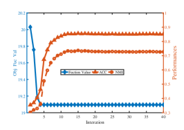
(a) Study on 3 Sources

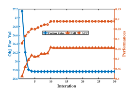
(b) Study on ORL

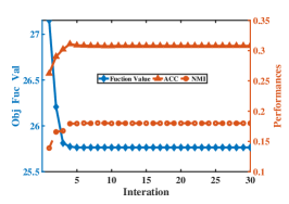
(c) Study on NUS

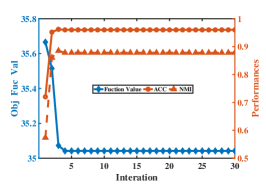
(d) Study on 20NGs

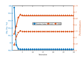
(e) Study on Scene

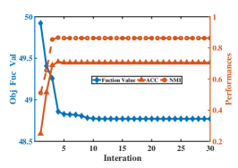
(f) Study on BBC

Figure 1: Convergence study on six datasets.

Following [18], we evaluate the results by three popular metrics: Accuracy (ACC), Normalized Mutual Information (NMI) and Purity.

4.3 Experimental Results

Table 2 to Table 4 shows the ACC, NMI and Purity values on six real-world datasets, respectively. Bold numbers denote the best result.

Results on 3 Sources dataset:

DSMC outperforms all the other methods significantly on 3 Sources. Specifically, compared with SwMC, we improve ACC by $38.47\%$, NMI by $61.32\%$, Purity by $40.83\%$. Relative to the latest method AWP, DSMC improves ACC by $8.29\%$, NMI by $9.90\%$, Purity by $5.92\%$. One possible reason for our outstanding clustering performance is that each view of 3 Sources dataset has a large number of important features, and our methods can effectively extract these important features.

Results on ORL dataset:

DSMC has better performances than the other methods on ORL. Obviously, compared with MMSC, DSMC improves ACC by $49.5\%$, NMI by $40.42\%$, Purity by $52.5\%$. Relative to AWP, it improves ACC by $6.00\%$, NMI by $2.31\%$, Purity by $6.75\%$. It is because each view of ORL has a large number of features, DSMC can distinguish the importance of these features by adaptively weighting them.

Results on NUS dataset:

DSMC outperforms all the other methods significantly on NUS. Especially, compared with MLAN, our DSMC improves ACC by $19.8\%$, NMI by $15.07\%$, Purity by $22.21\%$. Relative to the latest method AWP, DSMC improves ACC by $8.29\%$, NMI by $9.90\%$, Purity by $5.92\%$. The main reason is that NUS has $6$ views and our DSMC can effectively integrate favorable features from different graphs.

Results on 20NGs dataset:

For 20NGs dataset, DSMC obtains better clustering results than most of the other methods. Moreover, compared with MMSC, it improves ACC by $70.6\%$, NMI by $84.43\%$, Purity by $69\%$. Relative to the latest method AWP, DSMC improves ACC by $8.29\%$, NMI by $9.90\%$, Purity by $5.92\%$. The main reason for this phenomenon is that 20NGs dataset has many unfavorable features, which plays a negative role in learning optimal graphs. But our DSMC is able to remove these unfavorable features based on the weight matrix $M^{(v)}$. RMSC also achieves satisfactory clustering results. It is because each view of 20NGs has the same feature dimension (2000 features), which helps RMSC obtain the satisfactory Markov chain.

Results on Scene dataset:

Obviously, our proposed DSMC outperforms all the other methods significantly on Scene. In addition, compared with MMSC, DSMC improves ACC by $44.98\%$, NMI by $47.17\%$, Purity by $42.33\%$. AWP can achieve good clustering results because each view of this dataset contains a small number of features, which makes it easy for AWP to learn optimal Procrustes. Compared with AWP, our proposed DSMC improves ACC by $7\%$, NMI by $8\%$, Purity by $7\%$. This is mainly because DSMC is able to weigh different features through weight matrix $\bm{M}^{(v)}$, thereby extracting favorable features from views with different feature dimensions.

Results on BBC dataset:

When clustering BBC dataset, DSMC has better clustering performance than the other methods. Specifically, compared with SwMC, our proposed DSMC raises ACC by $61.75\%$, NMI by $65.93\%$, Purity by $62.17\%$. Relative to the latest method AWP, DSMC improves ACC by $16.79\%$, NMI by $10.7\%$, Purity by $15.92\%$. The main reason is that our DSMC can adaptively integrate different features multiple graphs fusion.

In summary, MMSC and SwMC often obtain poor clustering results. It is because they only learn one weight for different views, and do not take into account the local information on different features in each view. When clustering these datasets with a large number of instances (e.g., Scene and NUS), these local information will have a great impact on our clustering results. Meanwhile, although AWP can extract local information of the data, it cannot distinguish the importance of different features. Therefore, when we cluster multi-view data with high-dimensional features (e.g., BBC), AWP cannot obtain satisfactory results. By weighting different features, our proposed DSMC can effectively integrate different features, and adaptively fuse different graphs. Finally, DSMC always achieves the best performances among the compared state-of-the-art multi-view clustering methods.

4.4 Convergence Study

In Figure 1, we show the convergence curve, ACC values and NMI values w.r.t. the number of iterations. The blue solid curve indicates the value of the objective function and the dashed lines represent the clustering performance (ACC and NMI) of our proposed DSMC.

Obviously, for all the datasets, DSMC converges in less than $10$ steps, which proves the effectiveness and efficiency of our adaptive multiple graphs fusion. It is because after each iteration, DSMC can extract the favorable features of each view with the help of weight matrix $M^{(v)}$, and integrate different features of each view by $w_{v}$. When suitable weights are learned, the gradient of the objective function (Eq. (2.3)) is close to the ideal gradient, which accelerates the convergence of the objective function.

5 Conclusion

In this paper, we propose an effective dual self-weighted multi-view clustering framework, named DSMC. DSMC can remove redundant features and noises from each graph to improve clustering performance. In the framework of DSMC, we assign different weights to different features by imposing an adaptive weight factor. We design an adaptive multiple graphs fusion to fuse the features in the different views, thus integrating different graphs for clustering. We perform experiments on six real-world multi-view datasets to show the effectiveness and efficiency of our DSMC.

References

- [1] A. Blum and T. Mitchell, “Combining labeled and unlabeled data with co-training,” in Proceedings of the eleventh annual conference on Computational learning theory. ACM, 1998, pp. 92–100.
- [2] Z. Lu and Y. Peng, “Unified constraint propagation on multi-view data,” in Twenty-Seventh AAAI Conference on Artificial Intelligence, 2013.
- [3] C. Tang, X. Zhu, X. Liu, and L. Wang, “Cross-view local structure preserved diversity and consensus learning for multi-view unsupervised feature selection,” in AAAI Conference on Artificial Intelligence, 2019.
- [4] C. Lan and J. Huan, “Reducing the unlabeled sample complexity of semi-supervised multi-view learning,” in Proceedings of the 21th ACM SIGKDD International Conference on Knowledge Discovery and Data Mining. ACM, 2015, pp. 627–634.
- [5] C. Gong, J. Yang, and D. Tao, “Multi-modal curriculum learning over graphs,” ACM Transactions on Intelligent Systems and Technology (TIST), vol. 10, no. 4, p. 35, 2019.
- [6] S. Li, M. Shao, and Y. Fu, “Multi-view low-rank analysis with applications to outlier detection,” ACM Transactions on Knowledge Discovery from Data (TKDD), vol. 12, no. 3, p. 32, 2018.
- [7] W. Min, S. Jiang, S. Wang, J. Sang, and S. Mei, “A delicious recipe analysis framework for exploring multi-modal recipes with various attributes,” in ACM MM, 2017, pp. 402–410.
- [8] H. Wang, B. Chen, and W.-J. Li, “Collaborative topic regression with social regularization for tag recommendation,” in IJCAI, 2013.
- [9] Y. Wang, L. Zhou, J. Zhang, F. Zhai, J. Xu, C. Zong et al., “A compact and language-sensitive multilingual translation method,” 2019.
- [10] F. Nie, G. Cai, and X. Li, “Multi-view clustering and semi-supervised classification with adaptive neighbours,” in AAAI, 2017.
- [11] Z. Kang, X. Lu, J. Yi, and Z. Xu, “Self-weighted multiple kernel learning for graph-based clustering and semi-supervised classification,” in Proceedings of the 27th International Joint Conference on Artificial Intelligence. AAAI Press, 2018, pp. 2312–2318.
- [12] C. Du, C. Du, X. Xie, C. Zhang, and H. Wang, “Multi-view adversarially learned inference for cross-domain joint distribution matching,” in Proceedings of the 24th ACM SIGKDD International Conference on Knowledge Discovery & Data Mining. ACM, 2018, pp. 1348–1357.
- [13] L. Gao, H. Yang, J. Wu, C. Zhou, W. Lu, and Y. Hu, “Recommendation with multi-source heterogeneous information,” in IJCAI, 2018.
- [14] X. He, M.-Y. Kan, P. Xie, and X. Chen, “Comment-based multi-view clustering of web 2.0 items,” in WWW, 2014, pp. 771–782.
- [15] X. Cai, F. Nie, H. Huang, and F. Kamangar, “Heterogeneous image feature integration via multi-modal spectral clustering,” in CVPR 2011. IEEE, 2011, pp. 1977–1984.
- [16] R. Xia, Y. Pan, L. Du, and J. Yin, “Robust multi-view spectral clustering via low-rank and sparse decomposition,” in Twenty-Eighth AAAI Conference on Artificial Intelligence, 2014.
- [17] F. Nie, J. Li, X. Li et al., “Self-weighted multiview clustering with multiple graphs.” in IJCAI, 2017, pp. 2564–2570.
- [18] F. Nie, L. Tian, and X. Li, “Multiview clustering via adaptively weighted procrustes,” in Proceedings of the 24th ACM SIGKDD International Conference on Knowledge Discovery & Data Mining. ACM, 2018, pp. 2022–2030.
- [19] J. Friedman, T. Hastie, and R. Tibshirani, The elements of statistical learning. Springer series in statistics New York, 2001, vol. 1, no. 10.
- [20] S. Boyd, N. Parikh, E. Chu, B. Peleato, J. Eckstein et al., “Distributed optimization and statistical learning via the alternating direction method of multipliers,” Foundations and Trends® in Machine learning, vol. 3, no. 1, pp. 1–122, 2011.
- [21] J. Wen, Y. Xu, and H. Liu, “Incomplete multiview spectral clustering with adaptive graph learning,” IEEE transactions on cybernetics, 2018.
- [22] F. S. Samaria and A. C. Harter, “Parameterisation of a stochastic model for human face identification,” in Proceedings of 1994 IEEE workshop on applications of computer vision. IEEE, 1994, pp. 138–142.
- [23] T.-S. Chua, J. Tang, R. Hong, H. Li, Z. Luo, and Y. Zheng, “Nus-wide: a real-world web image database from national university of singapore,” in Proceedings of the ACM international conference on image and video retrieval, 2009, pp. 1–9.
- [24] L. Fei-Fei and P. Perona, “A bayesian hierarchical model for learning natural scene categories,” in 2005 IEEE Computer Society Conference on Computer Vision and Pattern Recognition (CVPR’05), vol. 2. IEEE, 2005, pp. 524–531.
- [25] D. Greene and P. Cunningham, “Practical solutions to the problem of diagonal dominance in kernel document clustering,” in Proceedings of the 23rd international conference on Machine learning. ACM, 2006, pp. 377–384.