Distributed Power Flow and Distributed Optimization – Formulation, Solution, and
Open Source Implementation

Abstract

Solving the power flow problem in a distributed fashion empowers different grid operators to compute the overall grid state without having to share grid models—this is a practical problem to which industry does not have off-the-shelf answers. In cooperation with a German transmission system operator we propose two physically consistent problem formulations (feasibility, least-squares) amenable to two solution methods from distributed optimization (the Alternating direction method of multipliers (admm), and the Augmented Lagrangian based Alternating Direction Inexact Newton method (aladin)); with aladin there come convergence guarantees for the distributed power flow problem. In addition, we provide open source matlab code for rapid prototyping for distributed power flow (rapidpf), a fully matpower-compatible software that facilitates the laborious task of formulating power flow problems as distributed optimization problems; the code is available under https://github.com/KIT-IAI/rapidPF/. The approach to solving distributed power flow problems that we present is flexible, modular, consistent, and reproducible. Simulation results for systems ranging from 53 buses (with 3 regions) up to 4662 buses (with 5 regions) show that the least-squares formulation solved with aladin requires just about half a dozen coordinating steps before the power flow problem is solved.

[Number of regions]nregionsn^reg [Set of regions]regionsR [Number of connections]nconnectionsn^conn [Number of core nodes]ncoren^core [Number of core nodes]ncopyn^copy [Number of buses]nbusn^bus

[Voltage phase angle]vangϕ [Voltage magnitude]vmagv [Active power]pp [Reactive power]qq

[State]statex [State of core node]stateCorex [State of copy node]stateCopyz

[Power flow problem]pfproblemg [Power flow equations]pfg^pf [Bus specifications]busspecsg^bus

[]DistOptLocalStateχ []DistOptUpdatedStateζ

1 Introduction

The power flow problem is the cornerstone problem for power systems analyses: find all (complex) quantities in an ac electrical network in steady state. The information drawn from the solution of the power flow problem is relevant for planning power systems, as well as expanding and operating them [1]. Hence, the power flow problem is relevant to all stakeholders maintaining a well-functioning electrical grid, most importantly transmission system operators (tsos) and distribution system operators (dsos). Traditionally, tsos and dsos solve and use power flow problems independently of each other, each making modeling assumptions with respect to the other system, e.g. treating the distribution system as a lumped load for the transmission system [2]. Clearly, these modeling assumptions—even if they were valid—may lead to real-world mismatches in both power and voltage. Hence—what is a sovereignty-preserving way to solve power flow problems for large power systems that may be composed of several tsos and/or dsos? This is the motivating question the present paper.

To answer this question we focus on the mathematical formulation and solution of the power flow problem. Mathematically, the power flow problem is modeled as a system of nonlinear equations, traditionally solved by Newton-Raphson methods or Gauss-Seidel approaches. These solution techniques may be classified as centralized approaches, i.e. the full grid model is available to a single central entity. This entity solves the power flow problem, having access to all information not just about the problem itself but also about the solution. Hence, this established approach is in principle able to solve power systems composed of tsos and dsos (so-called global power flow problems [2, 3])—but only at the cost of giving up sovereignty.

Recently, so-called distributed approaches have drawn significant academic attention. These are methods for which several entities (or agents) solve sub-problems independently of each other, then broadcast some—but not all—information to a coordinator [4, 5, 6, 7, 8]. The coordinator then solves a coordination problem, and sends to all entities the information they need to solve their sub-problems again. This process is repeated until convergence is achieved. The high-level description of distributed approaches suggests several advantages relative to centralized methods:

• distribute the computational effort,

• preserve sovereignty and/or privacy, e.g. grid models,

• decrease the vulnerability due to a single-point-of-failure, and

• add flexibility.

The interest in distributed approaches is not just academic; there exists a genuine desire by industry to leverage the advantages for real-world problems. In Germany, for example, the horizontal connection between the four tsos—50 Hertz, TenneT, Amprion, and TransnetBW—is based on centralized power flow solutions. However, new legislation and the undergoing German Energiewende toward more renewables force the German tsos to focus on new vertical cooperation with the numerous dsos. For this vertical cooperation, centralized approaches are not favorable mainly due to privacy concerns: the host then combines the role of data owner and product owner, and introduces a possible single-point-of-failure. Hence, it is not mainly the distributed computational effort, but more the increased privacy, reliability, and flexibility that spur the interest of tsos in distributed approaches.

Large Chinese cities are another example where the combined power flow problem for tsos and dsos is of relevance; in [2] it is argued that many Chinese cities are operating both transmission and distribution systems, both of which are studied and operated separately however. If a computational method were available to solve the combined power flow problem in terms of a privacy-preserving distributed problem, this would be helpful [2, 3].

In light of the above considerations the present paper contributes as follows:

1. We present two mathematical formulations of distributed power flow problems as privacy-preserving and physically-consistent distributed optimization problems.

2. We rigorously evaluate the applicability of the Alternating direction method of multipliers (admm)and the Augmented Lagrangian based Alternating Direction Inexact Newton method (aladin)to distributed power flow problems with up to several thousand buses.

3. We introduce rapidpf: open-source matlab code fully compatible with matpower that allows to generate matpower case files for distributed power flow problems tailored to distributed optimization; the code is available on https://github.com/KIT-IAI/rapidPF/ under the bsd-3-clause license.

4. We extend aladin-$\alpha$, a matlab rapid-prototyping toolbox for distributed and decentralized non-convex optimization, to allow for user-defined sensitivities and three new solver interfaces (fminunc, fminunc, worhp).

We explain our contributions relative to the state-of-the-art.

Ad c1: The idea to solve a global power flow problem that stands for the combination of tsos and dsos was popularized by the works [2, 3]. Specifically, [2] coined the term “Master-slave-splitting” to highlight the idea that there is a master system to which several workers are connected; also so-called “boundary systems” are introduced which make up the physical connection between the master and its worker [2]. The solution of the overall power flow problem is done iteratively: initialize the boundary voltages, solve the power flow for the worker systems, then substitute the solution to the boundary system, and solve the master system. This process is executed until the difference of voltage iterates is sufficiently small. Any power flow solver can be used to solve the sub-problems. Unfortunately, no convergence guarantees are provided, and the method was applied to systems with less than 200 buses.

In the follow-up work [3] a convergence analysis is carried out, but its practicability is limited due to mathematical settings—such as the implicit function theorem—that are difficult to relate to real-world criteria and/or data. Also, the simulation results from [3] are the ones from [2]. It hence remains unclear how well this method scales. Unfortunately, neither [2] nor [3] provide plots on the actual convergence behavior of their method, or wall-clock simulation times, or the influence of different initial conditions—all of which are aspects relevant to practitioners.

In light of [2, 3] the focus of the present paper is on the following:

• clear distinction between problem formulation and problem solution;

• two different mathematical problem formulations that make no assumptions on the sub-problems (e.g. meshed grids vs. radial grids);

• convergence properties follow from theory of distributed optimization;

• reproducible numerical results for test systems with up to $\approx$ 4000 buses.

Ad c2: Recently, distributed optimization techniques have drawn attention for distributed optimal power flow problems. It is especially admm that finds widespread application for optimal power flow [4, 9, 7]. However, admm being a first-order optimization methods often converges relatively quickly to the vicinity of the optimal solution, but then takes numerous iterations to approach satisfying numerical accuracy [10]. In addition, admm is known to be rather sensitive to both tuning and the choice of initial conditions [11]; line flow limits pose a significant obstacle for admm [4]. Furthermore, convergence guarantees for admm apply to convex optimization problems, but optimal power flow is known to be non-convex.

There exist distributed optimization methods that are devised for non-convex problems, for instance aladin. With aladin being a second-order method, it has access to curvature information that speed up convergence, at the expense of having to share more information among the sub-problems. The proof-of-concept applicability of aladin to distributed optimal power flow problems has been demonstrated in several recent works [12, 13, 8]; how to reduce the information exchange among the sub-problems is discussed in [14]. Compared to admm, aladin has more favorable convergence properties: within a few dozen iterations, convergence to the optimal solution is achieved with satisfying numerical accuracy [8]. Just like with admm, however, tuning remains a challenge with aladin. Also, the largest test case to which aladin was successfully applied is the 300-bus test case.

To summarize: both admm and aladin have demonstrated their potential for solving distributed optimal power flow problems. It is fair to ask how both methods apply to distributed power flow problems—a question that has not been tackled before to the best of the authors’ knowledge. Our findings suggest that for the distributed power flow problem aladin outperforms admm far more significantly than it does for the optimal power flow problem (in terms of scalability, speed, performance, and tuning). The main advantage of applying established techniques from distributed optimization to distributed power flow is that the convergence guarantees can be leveraged.

Ad c3: For academic power system analyses matpower is a mature, well-established, and widely adopted open source collection of matlab code [15]. It is not just the many computational facets that matpower provides that make it popular (power flow and several relaxations, optimal power flow, unit commitment, etc.), but also the so-called matpower case file format has inspired other open source packages, for instance PowerModels.jl [16] or PyPSA [17]. The matpower case file format describes a power system with respect to its bus data, generator data, and branch data. Additionally, there is a base MVA value for per-unit conversions, and for optimal power flow problems there is an entry on generator costs. Based on both the popularity and the maturity of matpower we provide glue code that solves the following laborious task: given several matpower case files, and given connection information for these case files, construct a matlab struct that corresponds to the mathematical problem formulation, and that is amenable to distributed optimization methods. This glue code is called rapidpf, and it is publicly available with a rich documentation—and full matpower compatibility. In addition, rapidpf decreases the time-from-idea-to-result, it computes relevant sensitivities (gradients, Jacobians, Hessians), and it comes with post-processing functionalities.

The idea of rapidpf is inspired by the matlab packages TDNetGen [18] and AutoSynGrid [19]; the code for rapidpf is hosted under https://github.com/KIT-IAI/rapidPF/. From a first glance, TDNetGen seems to provide functionality similar to rapidpf. As written in the abstract, TDNetGen is matlab code “able to generate synthetic, combined transmission and distribution network models” [18]. Unfortunately, TDNetGen is not as flexible as desired: there is currently no straightfoward way to generate TDNetGens so-called templates from arbitrary matpower case files. Also, the focus of TDNetGen is on generating large test systems, not on solving them. In turn, rapidpf allows to both generate test systems and prepare them for solution by distributed optimization methods such as admm and aladin. This preparation step must not be underestimated, because providing for an interface to distributed solvers is key in making distributed techniques more popular.

The focus of AutoSynGrid is on generating numerous test systems with similar statistical properties [19]. Hence, AutoSynGrid is not directly comparable to either TDNetGen or rapidpf.

Ad c4: The recently published matlab toolbox aladin-$\alpha$ provides several implementations of both admm and aladin [20]. Its user interface allows the user to provide merely the cost functions, the equality constraints, and the inequality constraints. Besides setting several default parameter settings, aladin-$\alpha$ computes derivatives required for either admm or aladin. To do so, aladin-$\alpha$ relies internally on casadi, an automatic differentiation framework that also parses the optimization problem to the low level interface of Ipopt [21, 22]. The idea of aladin-$\alpha$ is to provide rapid prototyping capabilities for general distributed optimization problems; it is not specifically tailored to distributed (optimal) power flow problems. From the authors’ experience, this all-purpose character in combination with casadi being hard-wired into aladin-$\alpha$ hinders it from being applicable to mid- to large-scale power flow problems.

We forked the code and tailored it to the needs of distributed power flow problems: the exact power flow Jacobian is passed from matpower, Hessian approximations are provided, and three new solvers are interfaced (fminunc, fminunc, worhp). Also, the interface of aladin-$\alpha$ needed substantial changes to allow for passing of user-supplied sensitivities instead of auto-computed sensitivities from casadi.

Although the motivation for the present paper is to solve power flow problems for systems composed of tsos and dsos, the authors stress that this setup is not a requirement. The presented methodology is generic in the following sense:

Given $i\in\{1,\ldots,\nregions\}$ power flow problems, and given suitable connection information, what is a coherent methodology for solving the overall power flow problem in a distributed manner?

It may be that the individual power flow problems happen to coincide with tsos and/or dsos, but they can as well be sub-problems of a genuinely large power flow problem that should be solved in a distributed way. In either case, the answer the present paper can provide to the above question is:

If the distributed power flow problem is formulated as a distributed-least squares problem, and if this problem is solved with aladin using a Gauss-Newton Hessian approximation, then the solution is found within half a dozen aladin iterations for systems ranging from 53 to 4662 buses.

Remark 1 (Partitioning).

The present paper assumes that the partitioning of the grid is given. For insights on how to partition large grids in computationally advantageous ways we refer to [23, 24, 25].

The paper is organized as its title suggests: formulation, solution, implementation, followed by an extensive section on results, and concluding comments. The formulation section 2 introduces nomenclature and the mathematical formulation of the distributed power flow problem. The solution section 3 covers two methods from distributed optimization: admm and aladin. The implementation is covered in section 4, with a strong focus on the open source matlab code rapidpf. The results section 5 gives both qualitative and quantitative assessments of the approach, clearly demonstrating that the least-squares formulation in combination with aladin is the most suitable solution approach. Concluding comments in section 6 close the paper.

2 Problem formulation

Given a single-phase equivalent of a connected AC electrical network in steady state with $\nbus\in\mathbb{N}$ buses, solving the power flow problems means to solve a set of nonlinear equations such that the complex voltage and apparent power of all buses of the network is found. The standard way to solve power flow problems is to apply a centralized method: a single machine determines the solution, for instance, via Gauss-Seidel or Newton-Raphson methods. An alternative is to distribute the computational effort to several machines, leading to so-called distributed approaches. Distributed approaches are promising because they eliminate single-point-of-failures, they better preserve privacy, their technical scale-up is easier, and they foster cooperation between transmission and distribution system operators. The idea of distributed power flow is to solve local power flow problems within each subsystem, independently of each other, and to find consensus on the physical values of the exchanged power between the subsystems, see 1(a).

2.1 Nomenclature

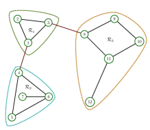
(a) Example how to decompose a power grid into three regions $\{1,2,3\}$, $\{4,5,6,7\}$, and $\{8,9,10,11,12\}$.

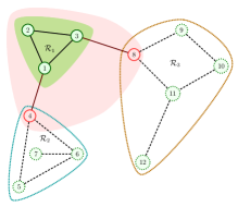
(b) From the perspective of region $\mathcal{R}_{1}$, the core buses are buses $\{1,2,3\}$, and the copy buses are buses $\{4,8\}$.

Figure 1: Graphical depiction of nomenclature for distributed power flow problems, see subsection 2.1.

Before we introduce suitable mathematical formulations for distributed power flow, we introduce some nomenclature. For that consider 1(a), which shows a 12-bus system divided into three subsystems (or so-called regions). Suppose we are the operator of region $\mathcal{R}_{1}=\{1,2,3\}$, for which we know all electrical parameters as well as all bus specifications, and for which we would like to solve a power flow problem. This requires additional information: the complex voltages of buses $\{4,8\}$, and the branch parameters of the tie lines—hence, connection information about the neighboring subsystems $\mathcal{R}_{2}=\{4,\ldots,7\}$ and $\mathcal{R}_{3}=\{8,\ldots,12\}$. We shall call buses $\{1,2,3\}$ the core buses of region $\mathcal{R}_{1}$, and buses $\{4,8\}$ the copy buses of region $\mathcal{R}_{1}$; 1(b) highlights the distinction. The combination of core buses and copy buses allows to formulate a self-contained power flow problem for every region.

Table 1: List of symbols for distributed power flow.

Symbol	Meaning
$\nregions$	Number of regions
$\nconnections$	Number of connecting lines between regions
$\ncore_{i}$	Number of core buses in region $i$
$\ncopy_{i}$	Number of copy buses in region $i$
$\stateCore_{i}$	Electrical state of core buses in region $i$
$\stateCopy_{i}$	Electrical state of copy buses in region $i$

2.2 Distributed power flow

Table 1 introduces the notation we use from here on: we consider a finite number $i\in\{1,\ldots,\nregions\}$ of regions. The (electrical) state $\stateCore_{i}$ of region $i$ contains the voltage angles, the voltage magnitudes, the net active power, and the net reactive power of all core buses

$$\stateCore_{i}=\begin{pmatrix}{\theta_{i}^{\text{core}}}&{v_{i}^{\text{core}}}&{p_{i}^{\text{core}}}&{q_{i}^{\text{core}}}\end{pmatrix}\in\mathbb{R}^{4\ncore_{i}}.$$ (1)

The (electrical) state $\stateCopy_{i}$ of region $i$ contains the voltage angles and the voltage magnitudes of all copy buses

$$\stateCopy_{i}=\begin{pmatrix}\theta_{i}^{\text{copy}}&v_{i}^{\text{copy}}\end{pmatrix}\in\mathbb{R}^{2\ncopy_{i}}.$$ (2)

Hence, each region $i$ is represented by a total of $4\ncore_{i}+2\ncopy_{i}$ real numbers. For all core buses of region $i$ the respective $2\ncore_{i}$ power flow equations $\pf_{i}\colon\mathbb{R}^{4\ncore_{i}}\times\mathbb{R}^{2\ncopy_{i}}\rightarrow\mathbb{R}^{2\ncore_{i}}$, and the respective $2\ncore_{i}$ bus specifications $\busspecs_{i}\colon\mathbb{R}^{4\ncore_{i}}\rightarrow\mathbb{R}^{2\ncore_{i}}$ make up the power flow problem for this very region [26]. Subtracting the number of equations from the number of decision variables gives a total of

$$\underbrace{4\ncore_{i}+2\ncopy_{i}}_{\text{Decision vars.}}-\underbrace{2\ncore_{i}}_{\text{Power flow eqns.}}-\underbrace{2\ncore_{i}}_{\text{Bus specs.}}=2\ncopy_{i}$$ (3)

missing equations per region $i$.

It remains to formalize the information that every copy bus from region $i$ corresponds to a core bus from a neighboring region $j\neq i$. An example: in 1(b), bus $4$ is a copy bus of region $\mathcal{R}_{1}$, and it is a core bus of region $\mathcal{R}_{2}$. Hence, their complex voltage must be identical.

Having introduced the nomenclature we formulate distributed power flow mathematically as follows

$$\pf_{i}(\stateCore_{i},\stateCopy_{i}) =0 \forall i\in\{1,\ldots,\nregions\}$$ (4a)

$$\busspecs_{i}(\stateCore_{i}) =0 \forall i\in\{1,\ldots,\nregions\}$$ (4b)

$$\sum_{i=1}^{\nregions}A_{i}\begin{bmatrix}\stateCore_{i}\\ \stateCopy_{i}\end{bmatrix} =0.$$ (4c)

The local power flow problem for region $i$ is given by (4a) and (4b), see Remark 2 and Remark 3; the so-called consensus matrices $A_{i}\in\mathbb{R}^{4\nconnections\times(4\ncore_{i}+2\ncopy_{i})}$ enforce equality of the voltage angle and the voltage magnitude at the copy buses and their respective core buses, hence they provide the remaining $4\nconnections=\textstyle\sum_{i=1}^{\nregions}2\ncopy_{i}$ missing equations, see footnote 9.

Remark 2 (Power flow equations).

The specific form of the regional power flow equations $\pf_{i}(\cdot)$ in (4) is arbitrary. Nevertheless, we chose polar coordinates for the voltage phasors when defining the electrical state in (1). In that case, the regional power flow equations are

$$p_{j} =v_{j}\sum_{k=1}^{n_{i}}v_{k}\left(G_{jk}\cos(\delta_{j}-\delta_{k})+B_{jk}\sin(\delta_{j}-\delta_{k})\right)$$ (5a)

$$q_{j} =v_{j}\sum_{k=1}^{n_{i}}v_{k}\left(G_{jk}\sin(\delta_{j}-\delta_{k})-B_{jk}\cos(\delta_{j}-\delta_{k})\right),$$ (5b)

for all buses $j$ from region $i$; the bus admittance matrix entries are $Y_{jk}=G_{jk}+\mathrm{j}B_{jk}$. For further details we refer to the excellent primer [27].

Remark 3 (Bus specifications).

For conventional power flow studies, each bus is modelled as one of the following:

• Slack bus: The voltage magnitude and the voltage angle are fixed; the net active and the reactive power are determined by the power flow solution.

• pq/load bus: The active power and the reactive power are fixed; the voltage magnitude and the voltage phasor are determined by the power flow solution.

• pv/voltage-controlled bus: The active power and the voltage magnitude are fixed; the reactive power and the voltage angle are determined by the power flow solution.

Mathematically, these requirements are simple equality constrains of the form $\busspecs_{i}(\cdot)$ for every region $i$.

Remark 4 (Physical consistence).

The concept of core buses and copy buses allows to compose the distributed power flow problem in a physically consistent manner: no additional modeling assumptions are introduced or required. If the solution to the distributed problem is found, then this is also the solution to the respective centralized power flow problem. In other words, copying buses does not introduce a structural numerical error [4].

Other approaches, such as “cutting” connecting tie lines and enforcing equality of the electrical state at the intersection [20], are in general not physically consistent (only in the absence of line capacitance). Hence, even if the true solution to the distributed problem is found, this solution is not numerically identical to the solution of the centralized power flow problem. In other words, cutting lines does introduce a structural numerical error, generally speaking.

Remark 5 (Privacy).

To formulate the power flow equations for region $i$, the voltage information of the copy buses needs to be shared among neighboring regions; this is inherent to the idea of core and copy buses. Although this means having to share data, the copy bus voltage data (i) does not contain a wealth of privacy information yet (ii) allows for a physically consistent problem formulation, see Remark 4.

2.3 Distributed optimization problem

The distributed power flow problem from (4) is a system of nonlinear equations. In contrast to the standard power flow problem, however, Problem (4) is in a form amenable to distributed optimization. Specifically, we propose to solve Problem (4) either as a distributed feasibility problem

$$\underset{\underset{\forall i\in\{1,\dots,\nregions\}}{\stateCore_{i},\stateCopy_{i}}}{\operatorname{min}}\>0\quad\operatorname{s.t.}$$ (6a)

$$\pf_{i}(\stateCore_{i},\stateCopy_{i}) =0$$ (6b)

$$\busspecs_{i}(\stateCore_{i}) =0$$ (6c)

$$\sum_{i=1}^{\nregions}A_{i}\begin{bmatrix}\stateCore_{i}\\ \stateCopy_{i}\end{bmatrix} =0,$$ (6d)

or as a distributed least-squares problem

$$\underset{\underset{\forall i\in\{1,\dots,\nregions\}}{\stateCore_{i},\stateCopy_{i}}}{\operatorname{min}}\sum_{i=1}^{\nregions}\>\left\lVert\begin{bmatrix}\pf_{i}(\stateCore_{i},\stateCopy_{i})\\ \busspecs_{i}(\stateCore_{i})\end{bmatrix}\right\rVert^{2}\quad\operatorname{s.t.}\quad\sum_{i=1}^{\nregions}A_{i}\begin{bmatrix}\stateCore_{i}\\ \stateCopy_{i}\end{bmatrix}=0.$$ (7)

Necessarily, the solution from the distributed feasibility problem is a solution for the distributed least-squares problem.

To summarize, we propose to formulate distributed power flow problems as either a distributed feasibility problem (6) or a distributed least-squares problem (7). Both formulations divide and conquer: formulate power flow problems for every region, and relate them by enforcing equal voltages at the connecting buses. The privacy overhead for the regional power flow problems is limited: only the voltage information of the connecting buses is required to formulate the regional power flow equations.

Both of the given formulations—feasibility (6) and least-squares (7)—are special cases of a more general problem formulation. We shall state the general problem formulation in order to simplify the solution algorithms to follow. Using

$$\regions=\{1,\ldots,\nregions\},$$ (8a)

we define

$$\underset{\underset{\forall i\in\regions}{\DistOptLocalState_{i}}}{\operatorname{min}}~{}\sum_{i\in\regions}f_{i}(\DistOptLocalState_{i})$$ (8b)

$$\text{subject to }\quad g_{i}(\DistOptLocalState_{i}) =0\qquad\forall i\in\regions$$ (8c)

$$\sum_{i\in\regions}A_{i}\DistOptLocalState_{i} =0,$$ (8d)

where $\DistOptLocalState_{i}=(\stateCore_{i},\stateCopy_{i})$ combines the core bus state and the copy bus state for region $i$. The consensus constraints (8d) are identical for either problem formulation; the correspondence of the cost and the equality constraints is summarized in the following Table 2.

Table 2: Correspondence of terms from general problem (8a) to feasibility problem (6) and to least-squares problem (7).

Term from (8a)	Feasibility problem (6)	Least-squares problem (7)
$f_{i}(\DistOptLocalState_{i})=$	0	$\left\lVert\begin{bmatrix}\pf_{i}(\stateCore_{i},\stateCopy_{i})\\ \busspecs_{i}(\stateCore_{i})\end{bmatrix}\right\rVert^{2}$
$g_{i}(\DistOptLocalState_{i})=$	$\begin{bmatrix}\pf_{i}(\stateCore_{i},\stateCopy_{i})\\ \busspecs_{i}(\stateCore_{i})\end{bmatrix}$	n/a

Remark 6 (Nonlinear least-squares problems [28]).

Least-squares have been studied extensively. Besides being an intuitive formulation of a problem at hand, least-squares problems provide rich structure that can be exploited. For nonlinear least-squares problems, it is well-known that Gauss-Newton methods work well. Instead of applying a full Gauss-Newton method we merely exploit the fact that the Hessian matrix can be approximated by the matrix product of the Jacobian.

3 Problem solution

Two viable methods to tackle distributed optimization problems of the form (6) or (7) are admm and aladin; we provide a brief overview of both. In the following, the superscript ^$k$ denotes the $k$^th iterate; the superscript ^$0$ hence denotes the initial condition.

Remark 7 (Wording).

Different problems bring about different wording. In the problem formulation in section 2 we speak of “regions”, because the power flow problem is usually related to an existing physical region. In the problem solution to follow, however, we prefer to speak of “subsystems”, and “local problems”, because the optimization problems that need to be solved in parallel need not resemble anything that exists in the physical world.

3.1 admm

The Alternating direction method of multipliers (admm)is a popular method for distributed optimization, particularly so for problems in context of power systems [4, 29, 9]. Although admm works often well in context of power systems, convergence is in general not guaranteed due to the non-convex ac power flow equations. We use admm as a benchmark method reflecting the current state-of-the-art for distributed optimization in power systems. Note that there exists a plethora of admm variants; the present paper relies on the formulation from [30]. We refer to [30, 10, 31] for more details on admm and its derivations and restrict ourselves to recalling the overall algorithm.

For problem (8a), admm is summarized in Algorithm 1. In step 1), admm solves local optimization problems, where the influence of the neighboring regions is incorporated via auxiliary terms in the objective function considering Lagrange-multiplier estimates $\lambda_{i}\in\mathbb{R}^{\nconnections}$ and estimates of the primal variables $\DistOptUpdatedState_{i}^{k}\in\mathbb{R}^{4\ncore_{i}+2\ncopy_{i}}$. In step 2), all local solutions $\DistOptLocalState_{i}^{k+1}$ are collected in a coordination problem. In many cases, this step can be simplified to a simple averaging step between neighboring subsystems [10]. Finally, the solution of the coordination problem $\DistOptUpdatedState_{i}^{k}$ is sent to each subsystem, and after a local Lagrange multiplier update—step 3)—the iterates start from the beginning.

Advantages of admm are its relatively small communication overhead, i.e. the necessity to communicate only the local solution between neighboring subsystems, and a relatively simple coordination, which consists of computing a simple average between neighboring subsystems.

Algorithm 1 admm for problem (8a)

Initialization: $\DistOptUpdatedState_{i}^{0},\lambda_{i}^{0}$ for all $i\in\mathcal{R}$, $\rho$
Repeat:

1. $\DistOptLocalState_{i}^{k+1}=\underset{g_{i}(\DistOptLocalState_{i})=0}{\operatorname{argmin}}\;f_{i}(\DistOptLocalState_{i})+\lambda_{i}^{k\top}A_{i}\DistOptLocalState_{i}+\frac{\rho}{2}\|A_{i}(\DistOptLocalState_{i}-\DistOptUpdatedState_{i}^{k})\|_{2}^{2},\;\;\,i\in\mathcal{R}$ (parallel)

2. $\DistOptUpdatedState^{k+1}=\underset{A\DistOptUpdatedState=0}{\operatorname{argmin}}\;\sum_{i\in\mathcal{R}}-\lambda_{i}^{k\top}A_{i}\DistOptUpdatedState_{i}+\frac{\rho}{2}\|A_{i}(\DistOptLocalState_{i}^{k+1}-\DistOptUpdatedState_{i})\|_{2}^{2}$ (centralized)

3. $\lambda_{i}^{k+1}=\lambda^{k}_{i}+\rho A_{i}(\DistOptLocalState_{i}^{k+1}-\DistOptUpdatedState_{i}^{k+1}),\qquad\qquad\qquad\qquad\qquad\qquad i\in\mathcal{R}$ (parallel)

Remark 8 (Local optimization problems).

Note that the local optimization problems in step 1) reflect the overall problem structure: in case of the distributed feasibility problem formulation (6), the local optimization problems comprise local feasibility problems, i.e. optimization problems with a zero cost and non-zero equality constraints; in case of the least-squares problem formulation (8a), the local problems are unconstrained nonlinear least-squares problems.

Remark 9 (admm for non-convex problems).

Recently, the convergence of admm has been shown in [32, 33] for special classes of non-convex problems. However, these works consider non-convexities in the objective function, whereas in case of the ac power flow equations the non-convexity appears in the constraints, for which to the best of our knowledge no convergence guarantee exists so far. Note that divergence of admm can occur also for very small-scale problems in context of power systems [34]; however, this is rarely observed.

3.2 aladin

As an alternative to admm, the Augmented Lagrangian based Alternating Direction Inexact Newton method (aladin)has been proposed [30]. Its main idea is to replace the relatively simple coordination step in admm with a more sophisticated one including also constraint and curvature information to yield fast and guaranteed convergence—also for problems with non-convex constraints.

aladin for problem (8a) is shown in Algorithm 2. Step 1) of aladin is similar to admm: each subsystem minimizes its own objective function with auxiliary terms. A minor difference is that aladin maintains one global Lagrange multiplier $\lambda$ only and that positive definite weighting matrices $\Sigma_{i}$ are considered in the augmentation term, where $\|x\|_{\Sigma}^{2}=x^{\top}\Sigma\,x$. In step 2), aladin then computes sensitivities of the local problems, i.e. the gradient of the cost function, $\nabla f_{i}^{\phantom{i}}(\DistOptLocalState_{i}^{k})$, an approximation of the Hessian of the Lagrangian function, $B_{i}^{k}$, and the Jacobian matrix of the constraints, $\nabla g_{i}(\DistOptLocalState_{i}^{k})$. These sensitivities are communicated to a central coordinator, which solves an equality-constrained quadratic program (qp) in step 3) of aladin. As a result, primal increments $\Delta\DistOptLocalState_{i}^{k}$ are communicated back to the subsystems, which update $\DistOptUpdatedState_{i}^{k}$ and $\lambda^{k}$ in step 4), and the iteration starts from the beginning.

In aladin, there are two tuning parameters: $\nu$ and $\rho$. The scaling matrices $\Sigma_{i}$ can be used for variable scaling—in case of well-behaved problems they can simply be set to the identity matrix. For details on selecting these parameters in context of power systems we refer to [8].

Algorithm 2 aladin for problem (8a)

Initialization: $\DistOptUpdatedState_{i}^{0},\lambda^{0}$, $\Sigma_{i}\succ 0$ for all $i\in\mathcal{R}$, $\nu,\rho$
Repeat:

1. Solve for all $i\in\mathcal{R}$

   $$\phantom{\Delta}\DistOptLocalState_{i}^{k}=\underset{g_{i}(\DistOptLocalState_{i})=0}{\operatorname{argmin}}\;f_{i}(\DistOptLocalState_{i})+\lambda^{k\top}A_{i}\DistOptLocalState_{i}+\frac{\nu}{2}\|\DistOptLocalState_{i}-\DistOptUpdatedState^{k}_{i}\|^{2}_{\Sigma},\qquad\qquad\qquad\quad\text{(parallel)}$$

2. Compute $\nabla f_{i}^{\phantom{i}}(\DistOptLocalState_{i}^{k})$, $\;B_{i}^{k}\approx\nabla_{\DistOptLocalState_{i}}^{2}\left(f_{i}^{\phantom{i}}(\DistOptLocalState_{i}^{k})+\gamma_{i}^{\top}g_{i}^{\phantom{i}}(\DistOptLocalState_{i}^{k})\right)$, $\;\nabla g_{i}(\DistOptLocalState_{i}^{k})$.

3. Solve the coordination qp
   

   $$\Delta\DistOptLocalState^{k}= \;\underset{\Delta\DistOptLocalState}{\operatorname{argmin}}\textstyle\sum_{i\in\mathcal{R}}\frac{1}{2}\Delta\DistOptLocalState_{i}^{\top}B_{i}^{k}\Delta\DistOptLocalState_{i}+\nabla f_{i}^{\top}(\DistOptLocalState_{i}^{k})\Delta\DistOptLocalState_{i}\qquad\qquad\qquad\;\;\text{(centralized)}$$

   $$+\lambda^{k\top}\left(\textstyle\sum_{i\in\mathcal{R}}A_{i}(\DistOptLocalState_{i}^{k}+\Delta\DistOptLocalState_{i})-b\right)+\frac{\rho}{2}\|\textstyle\sum_{i\in\mathcal{R}}A_{i}(\DistOptLocalState_{i}^{k}+\Delta\DistOptLocalState_{i})-b\|_{2}^{2}$$

   $$\text{subject to}\;\;\nabla g(\DistOptLocalState^{k})\Delta\DistOptLocalState=0.\qquad\qquad\qquad\qquad\qquad\qquad\quad\;\;\;$$

4. Set $\DistOptUpdatedState^{k+1}_{i}=\DistOptLocalState^{k}_{i}+\Delta\DistOptLocalState^{k}_{i}$ and $\lambda^{k+1}=\lambda^{k}+\rho\left(\sum_{i\in\mathcal{R}}A_{i}\DistOptLocalState_{i}-b\right).$ (parallel)

Remark 10 (Choosing Hessian approximations $B_{i}^{k}$).

aladin is guaranteed to converge locally for any positive definite Hessian approximation $B_{i}^{k}$ [30]. However, the domain of local convergence and especially the convergence rate depend on the quality of the approximation. Different Hessian approximations may also reduce the communication and computation overhead: for example, a Broyden-Fletcher-Goldfarb-Shanno (bfgs) approach is chosen in [8]. We study the influence of the choice of the Hessian approximation in subsubsection 5.2.2. Clearly, the choice of the Hessian should be motivated by the structure and nature of the local optimization problem, cf. Remark 8.

Remark 11 (Communication and coordination effort in aladin and admm).

In contrast to admm, aladin requires more communication and coordination per iteration compared with admm. The sensitivities $B_{i}^{k}$ and $\nabla g_{i}(\DistOptLocalState_{i}^{k})$ have to be communicated, whereas admm requires to communicate local decision variables $\DistOptLocalState_{i}^{k}$ only. Also the coordination step in aladin is more expensive: instead of computing simple averages, the coordination qp in step 3) of aladin requires solving a linear system of equations. With the help of this additional information, however, aladin converges faster than admm, hence partially compensating for the additional communication overhead. As an alternative to basic aladin, which is proposed here, one might consider using bi-level aladin [14]. Bi-level aladin is able to reduce the per-step communication and coordination overhead even further. We refer to [8, 14] for more detailed analytical and numerical comparisons.

4 Implementation

The problem formulations (section 2) and suggested solutions (section 3) are moot without means to actually implement, execute, and validate them. We introduce rapidpf, an open source matlab code that tackles the problem formulation, and we present an extension to aladin-$\alpha$, an open source matlab code that deals with the problem solution.

4.1 Rapid prototyping for distributed power flow (rapidpf)

Although there exist several excellent open-source tools to model, study, and solve (optimal) power flow problems (e.g. matpower in matlab [15], PowerModels in Julia [16], or pandapower in Python [35]), the same cannot be said for distributed (optimal) power flow problems—to the best of the authors’ knowledge. To help overcome both the tedious, error-prone, and laborious task of formulating distributed power flow problems, and of interfacing distributed optimization methods, we provide open source matlab code for rapidpf, which automates the following task:

Figure 2: Flow chart for rapidpf depicting its inputs (case files & connection information) and its output (matlab struct compatible with aladin-$\alpha$).

Given $\nregions$ matpower case files for all $i\in\{1,\ldots,\nregions\}$ regions, and given information about how the $i\in\{1,\ldots,\nregions\}$ regions are connected, generate a matlab struct compatible with aladin-$\alpha$.

The features of rapidpf span:

• Rapid prototyping: rapidpf decreases the time-from-idea-to-result.

• Compatibility: rapidpf is compatible with matpower and aladin-$\alpha$. All generated case files can be visualized, for example, with the excellent “Steady-State AC Network Visualization in the Browser”.

• Comparability: rapidpf generates matpower case files that can be validated by matpower functions such as runpf().

• Sensitivities: rapidpf generates function handles for gradients, Jacobians, and Hessians.

• Documentation: rapidpf comes with a self-contained and user-friendly online documentation.

• Open source: rapidpf is publicly available under the bsd-3-clause license on https://github.com/KIT-IAI/rapidPF/.

• Post-processing: rapidpf provides rich post-processing functionalities to analyze the results quickly and intuitively.

The code of rapidpf is made up of three components: the case file generator, the case file splitter, and the case file parser, see Figure 2. The case file generator requires as inputs several matpower case files in combination with their connection information; the connection information encodes who is connected to whom and by what (kind of branch and/or transformer). The regions can be connected in (almost) arbitrary ways, see Figure 3. The output of the case file generator is a matpower-compatible merged case file. This merged case file is generated for validation purposes: it provides a reference solution that can be computed, for instance, by running matpower’s runpf() command. The splitter adds information to each of the $\nregions$ case files about its core buses and copy buses. Finally, the parser takes the augmented case files, and generates an aladin-$\alpha$-compatible matlab struct that describes the problem either as a distributed feasibility problem (6) or as a distributed least-squares problem (7). The parser also generates sensitivities of the power flow problem, namely the Jacobian of the power flow equations and bus specifications as well as their Hessian information.

Remark 12 (Sensitivities).

All first- and second-order optimization methods require information about derivatives. Hence, rapidpf provides them for the user. The gradient of the local cost function, and the Jacobian of the power flow problem are the exact analytical expressions. The Hessian matrix—required only for aladin but not admm—is approximated by one of four methods: finite differences, bfgs, limited-memory bfgs, or Gauss-Newton. The first three methods can be applied to both problem formulations (feasibility (6) and least-squares (7)); Gauss-Newton is a method tailored to nonlinear least-squares problems [28], hence applies only to the least-squares formulation (7).

Remark 13 (Connecting buses).

A few more words are appropriate about how systems can be connected within the case file generator. First, we formally distinguish between the master system and its worker systems. The sole difference is that (without loss of generality) the slack bus of the overall system is the slack bus of the master system. The connection between two system is directed, imposing a natural distinction between the from- and to-system. For instance, consider the line connecting the Master and Worker 1 in Figure 3: the Master is the from-system, Worker 1 is the to-system. The connecting buses in both the from- and the to-system must be generation buses, hence either a slack bus or a pv bus. If the connecting bus in the to-worker-system is the slack bus, then this slack bus is replaced by a pq bus with zero generation and zero demand. If the connecting bus in the to-worker-system is a pv bus, then this pv bus is replaced by a pq bus with zero generation and its original demand. If no connecting bus in the to-worker-system is the slack bus, then the worker system’s slack bus is replaced by a pv bus; the respective set points for the active power and the voltage magnitude are taken from the matpower case file entries in mpc.gen.

Figure 3: Supported types of connections between regions.

4.2 Extensions to aladin-$\alpha$

Whereas rapidpf is matlab code tailored to simplify and streamline the problem formulation, the open source matlab code aladin-$\alpha$ is used to tackle the problem solution [20]. aladin-$\alpha$ provides tested implementations and several variants of both admm and aladin. Under the hood, aladin-$\alpha$ depends to a large degree on casadi—an open source tool for algorithmic differentiation—and Ipopt as the solver for nonlinear programs. Unfortunately, the sole dependency on casadi and Ipopt hinders distributed methods from aladin-$\alpha$ to be applicable to medium- to large-scale power systems (as we shall discuss in section 5). Hence, we created a separate branch for aladin-$\alpha$ that allows to use the user-defined sensitivities from rapidpf, and that allows to interface different solvers such as fmincon, fminunc, or worhp [36], see also the right-hand side of Figure 4.

5 Results

Figure 4: Problem formulation, problem solution, and interfaced solvers.

We turn to numerical results for power systems of various sizes. We examine several combinations of the two problem formulations—feasibility (6) and least-squares (7)—and the two solution methods—admm and aladin, paired with different ways to compute sensitivities and interfance different solvers, see Figure 4. The section is devised top-down: we begin with qualitative comparisons of admm and aladin, then examine the least-squares problem in combination with aladin (for different solvers and different Hessian approximations). The final section analyzes the convergence behavior for a 4662-bus system.

Our main finding is that the least-squares formulation with aladin and a Gauss-Newton Hessian approximation outperforms all other combinations.

Remark 14 (Settings common to all examples).

For all following examples, the connecting lines between all regions are modelled as transformers with a per-unit reactance of 0.00623, and a tap ratio of 0.985; the resistance, the total line charging susceptance, and the transformer phase shift angle are set to zero.

The initial condition for the primal state (i.e. the state of the electrical grid) is created from the matpower case files as follows: the voltage angle and voltage magnitude are initialized with their respective entries from the entries in the bus struct; similaly, the net active power and the net reactive power are initialized as the difference between the respective summed entries in the gen struct and the bus struct. All dual variables are set to 0.01 initially.

All computed solutions are verified relative to the reference solution provided by the matpower command runpf().

5.1 Qualitative comparison

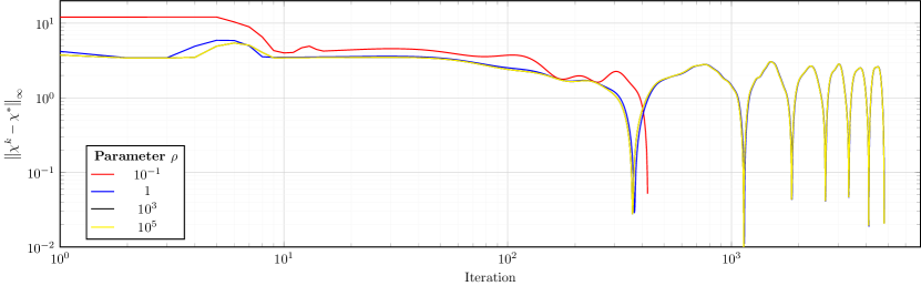
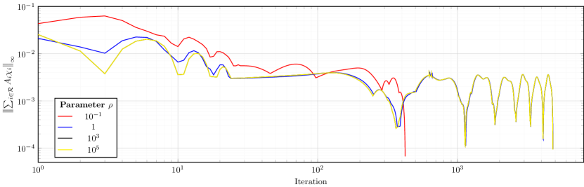
(a) Varying penalty parameter $\rho=10^{n}$ for $n\in\{-1,0,3,5\}$.

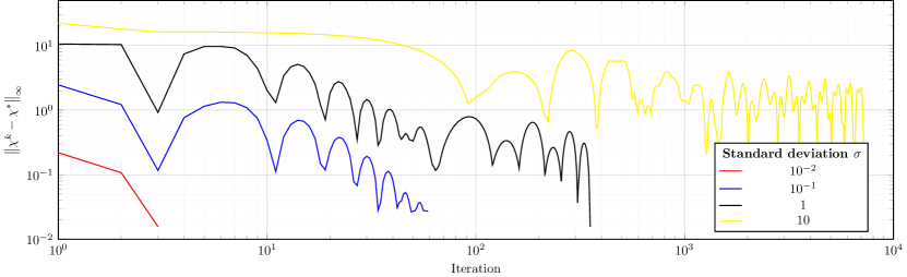
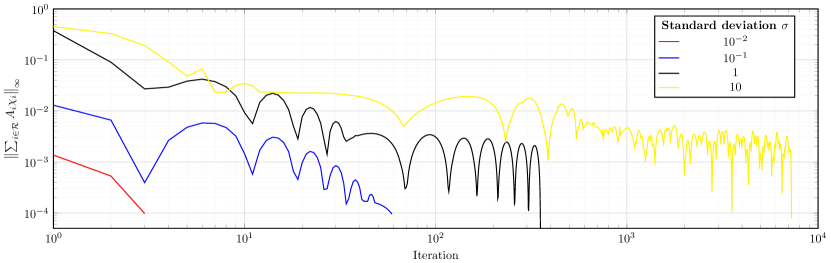
(b) Varying intial conditions $\DistOptLocalState^{\star}+\alpha\hat{\DistOptLocalState}$, where $\DistOptLocalState^{\star}$ is the true solution, $\hat{\DistOptLocalState}$ is a vector whose entries are samples from a standard normal distribution, and $\sigma\in\{0.01,0.1,1,10\}$ is the standard deviation.

Figure 5: Convergence behavior of admm for a feasibility problem formulation of the 53-bus test case from Table 4. In each subplot, the upper plot shows the distance to the optimal solution, and the lower plot shows the violation of the consensus constraints.

Table 3: Qualitative comparison of both problem formulations (feasibility vs. least-squares) and their solution by either admm or aladin.

	Feasibility problem (6)		Least-squares problem (7)
	admm	aladin	admm	aladin
Scalability	–	-	-	++
Speed	–	+	-	++
Performance	–	+	-	++
Tuning	–	-	-	+

We begin with a qualitative comparison of the applicability of both solution methods (admm and aladin) to both problem formulations (feasibility and least-squares); we base our qualitative findings on a total of 7 test cases that are summarized in the first four columns of Table 4.

From Table 3, which summarizes our qualitative findings, it appears that admm is unsuitable for either problem formulation. The performance of admm depends critically on both the choice of the penalty parameter and the initial condition. 5(a) shows the convergence behavior for admm applied to the feasibility formulation of the 53-bus test case from Table 4. For various choices of the penalty parameter $\rho$ admm exhibits strange and overall dissatisfying convergence properties. Most of the considered cases (the ones from Table 4) did not converge successfully even after having done significant parameter sweeps. 5(a) shows the influence of the choice of the penalty parameter $\rho$, and the often-encountered convergence behavior with admm: after relatively few iterations, the solution is in the vicinity of the optimal solution, but it takes several hundred iterations before further refinement occurs. And even then, the solution is far from being accurate. 5(b) shows the critical dependence on the (primal) initial condition: Perturbing the primal initial condition around the opimal solution, the plots show that the entire optimization process is prolonged significantly.

In contrast to admm, aladin appears applicable to solve the distributed power flow problems from Table 4. In all qualitative aspects we consider (scalability, speed, performance, tuning), the least-squares formulation outperforms the feasibility counterpart by far, see Table 3. It is especially the aspect of scalability that hinders the feasibility problem: for instance, the 354-bus test case from Table 4 already took 38.2 s to solve with fmincon, and converged within 14 aladin iterations.

An explanation for this behavior may be the zero-cost objective function for the feasibility problem (6); sensitivities of the objective hence contain no information. The advantage of the least-squares formulation is not just a non-zero objective function, but the absence of (in-)equality constraints in the local nonlinear programs, cf. Remark 8 and Remark 6.

5.2 Least-squares formulation with aladin

Based on our findings from the previous subsection 5.1, we consider only the least-squares formulation with aladin in what is to follow.

5.2.1 Different solvers

We investigate how the different solvers mentioned in Figure 2 cope with the different test cases from Table 4; we use the sensitivities provided by rapidpf in all cases, i.e. analytical gradients of the cost function, exact Jacobians, and the Gauss-Newton Hessian approximation.

Interestingly, Table 4 suggests that just half a dozen aladin iterations are sufficient to solve the test cases, which range from a total of 53 buses to 4662 buses. Hence, the applicability of aladin itself is clearly demonstrated. Of course, the overall solution time differs significantly with the choice of the local solver. As a negative result we find that plain aladin-$\alpha$, which interfaces only casadi with Ipopt, is not suitable for the problem at hand. That is why we chose to implement interfaces for the three other solvers: fminunc, fmincon, and worhp. Although fminunc is the seemingly best fit—the local subproblems are unconstrained optimization problems—its practical applicability is limited to subproblems of a few hundred buses. For the 2708- and 4662-bus test systems, fminunc takes significantly longer, because the dimension of the local subproblem grows too large. The solution times for fmincon and worhp are acceptable for all considered cases. It stands to reason that worhp will outperform fmincon for even larger test cases, because it is able to exploit the sparsity of the optimization problem.

Table 4: Computing times for different test cases and different solvers when solving the distributed least-squares problem (7) with aladin and sensitivities from rapidpf, see footnote 15.

		matpower		Solution time in s for			aladin
Buses		case files		fminunc	fmincon	worhp	iterations
53	3	9, 14, 30	3	2.5	2.2	2.4	4
354	3	3 $\times$ 118	5	2.5	3.1	4.8	5
418	2	118, 300	2	4.5	5.2	7.0	5
826	7	7 $\times$ 118	7	3.7	5.3	7.2	5
1180	10	10 $\times$ 118	11	4.9	6.7	9.8	6
2708	2	2 $\times$ 1354	1	212.7	41.9	53.6	4
4662	5	3 $\times$ 1354, 2 $\times$ 300	4	387.9	90.1	113.8	5

5.2.2 Different Hessian approximations

With aladin being a second-order optimization method, the Hessian matrix is required—or an accurate yet easy-to-compute approximation thereof. We compare four different Hessian approximations for the least-squares problem (7) with aladin: finite differences, bfgs, limited-memory bfgs, and the Gauss-Newton method. The results, which are shown in Table 5, confirm what is to be expected: the Gauss-Newton method outperforms all other methods. This is in accordance with the fact that exploiting the structure of the least-squares formulation correctly pays off tremendously. The finite difference approximation, just like the two bfgs methods, are all-purpose Hessian approximation unaware of the underlying problem structure. Gauss-Newton, in turn, is a Hessian approximation tailored to nonlinear least squares problem, see also Remark 12. The results from Table 5 make it clear that already for small system sizes, the all-purposes Hessian approximations should be avoided, because they lead to longer computation times. Consequently, the default Hessian approximation for least-squares problems is the Gauss-Newton method in rapidpf.

Table 5: Computing times for least-squares problem (7) with aladin and fmincon, for different Hessian approximations. The entries in the column “Buses” refers to the entries in Table 4.

Buses	Finite difference	bfgs	Limited-memory bfgs	Gauss-Newton
53	10.0	28.6	22.9	2.2
354	61.5	287.8	107.4	3.1
418	185.6	1086.4	148.2	5.2
826	n/a	n/a	n/a	5.3
$\ldots$	n/a	n/a	n/a	See Table 4
4662	n/a	n/a	n/a	See Table 4

5.3 4662-Bus system – Convergence behavior

Next, we study the convergence behavior of the 4662-bus test case. This test case is composed of three 1354-bus matpower test cases, and two 300-bus matpower test cases. Table 6 shows the connecting buses between the regions. For other relevant information such as how the connecting lines are modelled, and how the initial conditions are chosen, see Remark 14.

To solve the distributed power flow problem we choose a least-squares formulation with aladin. We use the Gauss-Newton Hessian approximation, and fmincon is used to solve the local problems. From Table 4 we see that this setup requires 5 aladin iterations and about 90 seconds. Figure 6 shows, for every aladin iteration and for every region, the $\infty$-norm of the power flow equations (4a), of the bus specifications (4b), and of the consensus constraint violations (4c). After 5 aladin iterations, all violations are below $10^{-10}$, and the computations are terminated.

Table 6: Regions and used test cases for 4662-bus test case (left). Connecting buses between regions (middle). Connection graph (right)

Region matpower case file 1 case1354pegase 2 case1354pegase 3 case1354pegase 4 case300 5 case300

From-system To-system Region Bus Region Bus 1 17 2 46 1 111 3 271 2 64 4 10 2 837 5 8

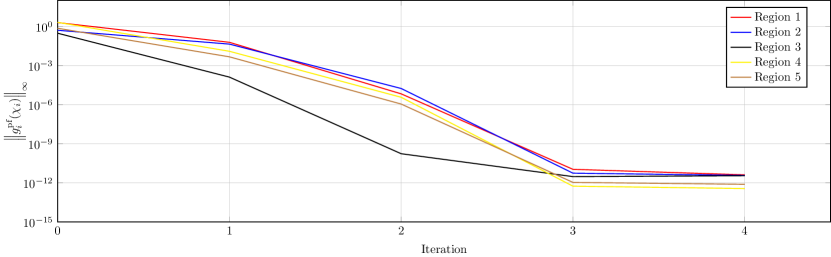
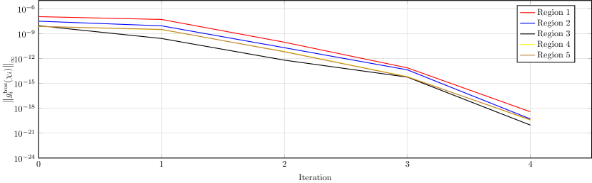
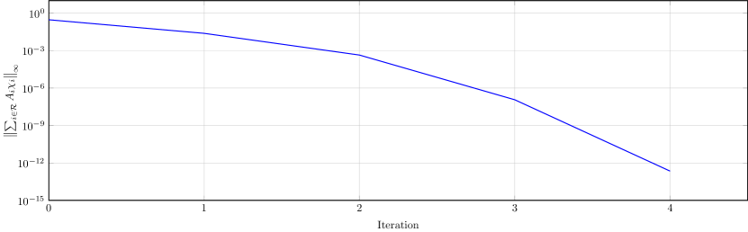
Figure 6: Decrease of the $\infty$-norm of the power flow equations, the bus specifications, and the consensus violations, each per aladin iteration for the 4662-bus system from Table 4.

6 Conclusion & Outlook

The relevance of distributed power flow problems is increasing, because their solutions allow for better cooperation between different stakeholders, e.g. tsos and dsos. Distributed optimization is a viable technique to tackle such distributed power flow problems. It is speficically the Augmented Lagrangian based Alternating Direction Inexact Newton method (aladin)with its convergence guarantees that yields promising results: if the distributed power flow problem is formulated as a distributed least-squares problem, and if a Gauss-Newton Hessian approximation is used, then about half a dozen iterations suffice to converge to the correct solution. To facilitate rapid prototyping we introduce rapid prototyping for distributed power flow (rapidpf), which is fully matpower-compatible matlab code that takes over the laborious task of creating code amenable to distributed optimization.

Future steps will focus mainly on further structure exploitation for solving the problem, and on implementing larger test cases. The least-squares formulation is promising, hence further improvements are possible, such as relying not on an all-purpose solver but devising a solver dedicated to nonlinear-least squares problems. A first step might be a tailored Gauss-Newton method, or a tailored Levenberg-Marquardt method [28]. For the Gauss-Newton method, for example, it is possible to avoid having to compute the Hessian altogether, because a singular-value decomposition or a conjugate gradient method can be applied directly to solve the linearized problem [28]. This user-defined nonlinear-least squares solver must then be interfaced with aladin-$\alpha$.

The simulation results we presented are all carried out on a single machine. To leverage the literal distribution of the optimization, efforts toward parallel computing shall be undertaken when tackling larger test cases.

Finally, rapidpf can be extended to optimal power flow problems upon adding cost functions per region.

Contributor roles

See Table 7 for the roles of each author.

Table 7: Contributor roles.

Author	Role(s)
Tillmann Mühlpfordt	Conceptualization, investigation, methodology, software, writing – original draft
Xinliang Dai	Software, investigation, visualization
Alexander Engelmann	Methodology (while at kit), writing – original draft (subsection 3.1, subsection 3.2) (while at tu Dortmund)
Veit Hagenmeyer	Conceptualization, funding acquisition, writing – review & editing

References

- [1] J. Grainger, W. Stevenson, Power System Analysis, McGraw-Hill Education, 1994.
- [2] H. Sun, B. Zhang, Distributed power flow calculation for whole networks including transmission and distribution, in: 2008 IEEE/PES Transmission and Distribution Conference and Exposition, 2008, pp. 1–6.
- [3] H. Sun, Q. Guo, B. Zhang, Y. Guo, Z. Li, J. Wang, Master–slave-splitting based distributed global power flow method for integrated transmission and distribution analysis, IEEE Transactions on Smart Grid 6 (3) (2015) 1484–1492. doi:10.1109/TSG.2014.2336810.
- [4] T. Erseghe, Distributed Optimal Power Flow Using ADMM, IEEE Transactions on Power Systems 29 (5) (2014) 2370–2380.
- [5] B. H. Kim, R. Baldick, Coarse-grained distributed optimal power flow, IEEE Transactions on Power Systems 12 (2) (1997) 932–939.
- [6] G. Hug, S. Kar, C. Wu, Consensus + Innovations Approach for Distributed Multiagent Coordination in a Microgrid, IEEE Transactions on Smart Grid 6 (4) (2015) 1893–1903.
- [7] B. Kim, R. Baldick, A comparison of distributed optimal power flow algorithms, IEEE Transactions on Power Systems 15 (2) (2000) 599–604.
- [8] A. Engelmann, Y. Jiang, T. Mühlpfordt, B. Houska, T. Faulwasser, Toward distributed OPF using ALADIN, IEEE Transactions on Power Systems 34 (1) (2019) 584–594. doi:10.1109/TPWRS.2018.2867682.
- [9] J. Guo, G. Hug, O. K. Tonguz, A case for nonconvex distributed optimization in large-scale power systems, IEEE Transactions on Power Systems 32 (5) (2017) 3842–3851.
- [10] S. Boyd, N. Parikh, E. Chu, B. Peleato, J. Eckstein, Distributed optimization and statistical learning via the alternating direction method of multipliers, Foundations and Trends® in Machine Learning 3 (1) (2011) 1–122.
- [11] A. X. Sun, D. T. Phan, S. Ghosh, Fully decentralized AC optimal power flow algorithms, in: 2013 IEEE Power Energy Society General Meeting, 2013, pp. 1–5.
-
[12]
A. Engelmann, T. Mühlpfordt, Y. Jiang, B. Houska, T. Faulwasser,