Multifractal analysis of sums of random pulses

Abstract.

In this paper, we determine the almost sure multifractal spectrum of a class of random functions constructed as sums of pulses with random dilations and translations. In addition, the continuity modulii of these functions is investigated.

1. Introduction

Multifractal analysis aims at describing those functions or measures whose pointwise regularity varies rapidly from one point to another. Such behaviors are commonly encountered in various mathematical fields, from harmonic and Fourier analysis (reference) to stochastic processes and dynamical systems [4, 5, 6, 30, 33, 34]. Multifractality is actually a typical property in many function spaces [9, 14, 15, 32]. Multifractal behaviors are also identified on real-data signals coming from turbulence, image analysis, geophysics for instance [24, 25, 1]. To quantify such an erratic behavior for a function $f\in L_{loc}^{\infty}(\mathbb{R})$, it is classically called for the notion of pointwise Hölder exponent defined in the following way.

Definition 1.1.

Let $f\in L^{\infty}_{loc}(\mathbb{R})$, $x_{0}\in\mathbb{R}$ and $\alpha\geq 0$. A function $f$ belongs to $C^{\alpha}(x_{0})$ when there exist a polynomial $P_{x_{0}}$ of degree less than $\lfloor\alpha\rfloor$ and $K_{\alpha}\in\mathbb{R}_{+}^{*}$ such that

$$\exists r\in\mathbb{R}_{+}^{*},\ \forall x\in B(x_{0},r),\ |f(x)-P_{x_{0}}(x-x_{0})|\leq K_{\alpha}|x-x_{0}|^{\alpha}.$$

The pointwise Hölder exponent of $f$ at a point $x_{0}$ is defined by

$$h_{f}(x_{0})=\sup\{\alpha\geq 0:\ f\in C^{\alpha}(x_{0})\}.$$

In order to describe globally the pointwise behavior of a given function of a process, let us introduce the following iso-Hölder sets.

Definition 1.2.

Let $f\in L^{\infty}_{loc}(\mathbb{R})$ and $h\geq 0$. The iso-Hölder set $E_{f}(h)$ is

$$E_{f}(h)=\{x\in\mathbb{R}:\ h_{f}(x)=h\}.$$

The functions studied later in this paper have fractal, everywhere dense, iso-Hölder sets. It is therefore relevant to call for the Hausdorff dimension, denoted by $\dim_{\!H}$, to distinguish them, leading to the notion of multifractal spectrum.

Definition 1.3.

The multifractal spectrum of $f\in L^{\infty}_{loc}(\mathbb{R})$ on a Borel set $A\subset\mathbb{R}$ is the mapping defined by

$$D^{A}_{f}:\left\{\begin{array}[]{lcl}\mathbb{R}_{+}&\longrightarrow&\mathbb{R}_{+}\cup\{-\infty\}\\ h&\longmapsto&\dim_{\!H}(E_{h}\cap A).\end{array}\right.$$

By convention, $\dim_{\!H}(\emptyset)=-\infty$. The multifractal spectrum of a function or a stochastic process $f$ provides one with a global information on the geometric distribution of the singularities of $f$.

In this article, we aim at computing the multifractal spectrum of a class of stochastic processes consisting in sums of dilated-translated versions of a function (referred to as a ”pulse”) that can have an arbitrary form. The translation and dilation parameters are random in our context. The present article hence follows a longstanding research line consisting in studying the regularity properties of (irregular) stochastic processes that can be built by an additive construction, including for instance additive Lévy processes, random sums and wavelet series, random tesselations, see [31, 38, 33, 26, 27] amongst many references.

Our model is particularly connected to other models previously introduced and studied by many authors.

For instance, in [39] Lovejoy and Mandelbrot modeled rain fields by a 2-dimensional sum of random pulses constructed as follows. Consider a random Poisson measure $N$ on $E=\mathbb{R}_{+}^{*}\times\mathbb{R}_{+}^{*}\times\mathbb{R}^{d}$, as well as a ”father pulse” $\psi:\mathbb{R}^{d}\to\mathbb{R}$, $\alpha\in]0,2[$ and $\eta\in]0,1]$. Lovejoy and Mandelbrot built and studied the process $M:\mathbb{R}^{d}\to\mathbb{R}$ defined by

(1) $$M(x)=\int_{(\lambda,w,\tau)\in E}\lambda^{-\alpha}\psi(w^{\frac{1}{\eta}}(x-\tau))N(d\lambda,dw,d\tau)=\sum_{(\lambda,w,\tau)\in S}\lambda^{-\alpha}\psi_{\lambda,w,\tau}(x),$$

where $S$ is the set of random points induced by the Poisson measure and $\psi_{\lambda,w,\tau}(x):=\psi(w^{\frac{1}{\eta}}(x-\tau))$ and $\eta=1$.

In [17], Cioczeck-Georges and Mandelbrot showed that negatively correlated fractional Brownian motions ($0<H<1/2$) can be obtained as a limit (in the sense of distributions) of a sequence of processes defined as in (1) with $\psi$ a well-chosen jump function, $\alpha\in]0,2[$ and $\eta=1$. Later, in [18], the same authors proved that any fractional Brownian motion with Hurst index $H\in(0,1)\setminus\{1/2\}$ is a limit of a sequence of processes $\{M_{n}(x),x\geq 0\}_{n\in\mathbb{N}}$ defined as in (1) with $\psi$ a conical or semi-conical function. Other versions with general pulses $\psi$ have been investigated in [40].

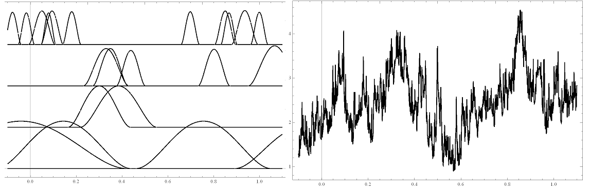
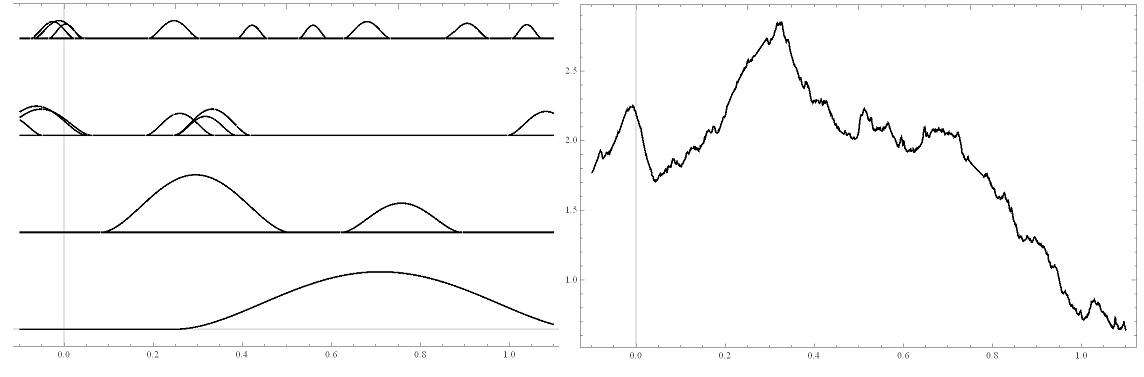
Figure 1. Two sample paths obtained with different pulses and parameters

In [19], Demichel studied a model in which only the position coefficients $(X_{n})_{n\geq 1}$ are random : the corresponding model is written

(2) $$G(x)=\sum_{n=1}^{+\infty}a_{n}\psi(\lambda_{n}^{-1}(x-X_{n})),\ \ \ x\in\mathbb{R}$$

where $(a_{n})_{n\in\mathbb{N}^{*}}$ and $(\lambda_{n})_{n\in\mathbb{N}^{*}}$ are two deterministic positive sequences such that $\sum\limits_{n\in\mathbb{N}^{*}}a_{n}=+\infty$ and $(\lambda_{n})_{n\in\mathbb{N}^{*}}$ is decreasing to $0$, and $X_{n}\sim U([0,1])$ is an i.i.d. sequence of random variables. The same example is developed in [21, 20] where Demichel, Falconer and Tricot impose that $a_{n}=n^{-\alpha}$ with $0<\alpha<1$, $\lambda_{n}=n^{-1}$, and $\psi:\mathbb{R}\rightarrow\mathbb{R}$ is an even, positive continuous function, decreasing on $[0,1]$, equal to 0 on $[1,+\infty[$ satisfying $\psi(0)=1$.
Calling $\Gamma_{G}$ the graph of the process $G$ and $\dim_{B}\Gamma_{G}$ its box-dimension, they showed that as soon as there exists an interval $I$ on which $\psi\in\mathcal{C}^{H}(\mathbb{R})$ (the space of global Hölder real functions of exponent $H$) and is $\mathcal{C}^{1}$-diffeomorphic on some interval, then almost surely

(3) $$2-\alpha\leq\dim_{\!H}(\Gamma_{G})\leq\dim_{B}(\Gamma_{G})\leq 2-\min\{\alpha,h\}.$$

See also [3] for the box dimension of $\Gamma_{G}$, or [42, 44] for a more systematic study of graph dimensions. When $\alpha<h$, almost surely $\dim_{\!H}(\Gamma_{G})=\dim_{B}(\Gamma_{G})=2-\alpha$. In [10], Ben Abid gave alternative conditions for the convergence of such processes $G$, also determining the uniform regularity of $G$, i.e. to which global Hölder space $\mathcal{C}^{H}(\mathbb{R})$ $G$ may belong to, almost surely.

Our purpose is to study another, somehow richer, model of sums of random pulses.

2. A model with additional randomness

The stochastic processes $F$ considered in this article are natural extensions of the previous models, and fit in the general study of pointwise regularity properties of rough sample paths of stochastic processes. As in the aforementioned works, we obtain results regarding their existence and regularity properties. We go further by providing a complete multifractal analysis of $F$ and by investigating various modulii of continuity.

Fix a probability space $(\Omega,\mathcal{F},\mathbb{P})$ on which all random variables and stochastic processes are defined.

Let $(C_{n})_{n\in\mathbb{N}^{*}}$ be a point Poisson process whose intensity is the Lebesgue measure on $\mathbb{R}_{+}$, and let $S$ be another point Poisson process, independent with $(C_{n})_{n\in\mathbb{N}^{*}}$, whose intensity is the Lebesgue measure on $\mathbb{R}_{+}^{*}\times[0,1]$. We write $S=(B_{n},X_{n})_{n\in\mathbb{N}^{*}}$ where the sequence $(B_{n})_{n\in\mathbb{N}^{*}}$ is increasing. By construction, the three sequences of random variables $(C_{n})$, $(B_{n})$ and $(X_{n})$ are mutually independent.

Definition 2.1.

Let $\psi:\mathbb{R}\rightarrow\mathbb{R}$ be a Lipschitz function with support equal to $[-1,1]$, $\alpha\in(0,1)$ and $\eta\in(0,1)$. The (random) sum of pulses $F$ is defined by

(4) $$F(x)=\sum_{n=1}^{+\infty}C_{n}^{-\alpha}\psi_{n}(x),\ \ \mbox{ where }\ \ \psi_{n}(x):=\psi(B_{n}^{\frac{1}{\eta}}(x-X_{n}))$$

The parameter $\alpha$ will be interpreted as a regularity coefficient, and $\eta$ as a lacunarity coefficient. Observe that the support of $\psi_{n}$ is the ball $B(X_{n},B_{n}^{-1/\eta})$ ($B(t,s)$ stands for the ball with centre $t$, radius $s$).

The stochastic process $F$ possesses interesting properties on the interval $[0,1]$ only, since $X_{n}\in[0,1]$. However, this is not a restriction at all, since $F$ can easily be extended to $\mathbb{R}$ as follows.

For every integer $m$, consider $F_{m}$, an independent copy of $F$ but shifted by $m$. Then,

$$\widetilde{F}:=\sum_{m\in\mathbb{Z}}F_{m}$$

enjoys the same pointwise regularity properties as $F$. It is interesting to see that this new process $\widetilde{F}$ has now stationary increments, and enlarges the quite narrow class of stochastic processes with stationary increments whose multifractal analysis is completely understood.

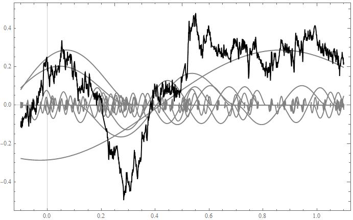
Figure 2. Sample path of $F$ computed with 1000 dilated and translated pulses

In [33], using for $\psi$ a smooth wavelet generating an orthonormal basis, S. Jaffard studied the lacunary random wavelet series

$$W(x)=\sum_{j\in\mathbb{N}}\sum_{k\in\mathbb{Z}}C_{j,k}2^{-j\alpha}\psi_{j,k}(x),\ \ \ x\in\mathbb{R},$$

where for all $(j,k)\in\mathbb{N}\times\mathbb{Z}$, $\psi_{j,k}(x)=\psi(2^{j}x-k)$ and the wavelet coefficients $C_{j,k}$ are independent random variables wavelets whose law is a Bernoulli measure with parameter $2^{-j\eta}$ (hence, depending on $j$ only). The main difference between the lacunary wavelet series and our model (motivating our work) is that not only dilations $(B_{n})_{n\in\mathbb{N}^{*}}$ but also the translations $(X_{n})_{n\in\mathbb{N}^{*}}$ are random in our case. Hence our interest in $F$ (and in $\widetilde{F}$) comes from the fact that it is not based on a dyadic grid, hence providing one with a homogeneous model more natural from a probabilistic point of view, the process $\widetilde{F}$ having stationary increments. The main results of this article concern the global and pointwise regularity properties of $F$, which are proved to be similar to those of $W$.

We start by the multifractal properties of $F$.

Theorem 2.1.

Let $F$ be as in Definition 2.1. With probability one, one has

$$D^{[0,1]}_{F}(H)=\left\{\begin{array}[]{lcr}\frac{H}{\alpha}&\mbox{if}&H\in[\alpha\eta,\alpha],\\ -\infty&\mbox{ else.}\end{array}\right.$$

The other results concern the almost-sure global regularity of $F$ and its modulii of continuity. Let us recall the notions of modulus of continuity.

Definition 2.2.

A non-zero increasing mapping $\theta:\mathbb{R}^{+}\to\mathbb{R}$ is a modulus of continuity when it satisfies

1. $\theta(0)=0$,

2. There exists $K>0$ such that for every $h\geq 0$, $\theta(2h)\leq K\theta(h)$.

Function spaces are naturally associated with modulii of continuity.

Definition 2.3.

A function $f\in L^{\infty}_{loc}(\mathbb{R})$ has $\theta:\mathbb{R}^{+}\to\mathbb{R}$ as uniform modulus of continuitywhen there exists $K>0$ such that

$$\forall h\in\mathbb{R}_{+},\ w_{f}(h):=\sup_{|x-y|\leq h}|f(x)-f(y)|\leq K\theta(h).$$

A function $f\in L^{\infty}_{loc}(\mathbb{R})$ has $\theta:\mathbb{R}^{+}\to\mathbb{R}$ as local modulus of continuity at $x_{0}\in\mathbb{R}$ when there exist $\eta_{x_{0}}>0$ and $K_{x_{0}}>0$ such that

(5) $$\forall x\mbox{ such that }|x-x_{0}|\leq\eta_{x_{0}},\ \ \ \ |f(x)-f(x_{0})|\leq K_{x_{0}}\theta(|x-x_{0}|).$$

A function $f\in L^{\infty}_{loc}(\mathbb{R})$ has $\theta:\mathbb{R}^{+}\to\mathbb{R}$ as almost-everywhere modulus of continuity when $\theta$ is a local modulus of continuity for $f$ at Lebesgue almost every $x_{0}\in\mathbb{R}$.

When $\alpha\in(0,1)$ and $\theta(h)=\theta_{\alpha}(h):=|h|^{\alpha}$, the functions having $\theta_{\alpha}$ as uniform modulus of continuity is exactly the set $\mathcal{C}^{\alpha}(\mathbb{R})$ of $\alpha$-Hölder functions (to deal with exponents $\alpha\geq 1$, the definition of $w_{f}(h)$ must be modified and use finite differences of higher order).

Our result theorem regarding continuity moduli is the following.

Theorem 2.2.

Let $F$ be as in Definition 2.1. With probability 1:

1. Tthe mapping $h\mapsto|h|^{\alpha\eta}|\log_{2}(h)|^{2+\alpha}$ is a uniform modulus of continuity of $F$.

2. The mapping $h\mapsto|h|^{\alpha}|\log_{2}(h)|^{2+\alpha}$ is an almost everywhere modulus of continuity of $F$.

3. At Lebesgue almost every $x_{0}\in[0,1]$, the local modulus of continuity of $F$ at $x_{0}$ is larger than $h\mapsto|h|^{\alpha}|\log_{2}(h)|^{2\alpha}$.

Remark 1.

Items (ii) and (iii) above provide us with a tight window for the optimal almost everywhere modulus of continuity $\theta_{F}$ of $F$, i.e.

$$|h|^{\alpha}|\log_{2}(h)|^{2\alpha}\leq\theta_{F}(h)\leq|h|^{\alpha}|\log_{2}(h)|^{2+\alpha}.$$

The investigation of a sharper estimate for this modulus of continuity is certainly of interest. For instance, S. Jaffard was able to obtain a precise characterization in the case of lacunary wavelet series, see Theorem 2.2 of [33].

Remark 2.

The result can certainly be extended to dimension $d>1$ with parameters $\alpha>1$, provided that $\psi\in C^{\lfloor\alpha\rfloor+1}(\mathbb{R}^{d})$. This would add technicalities not developed here.

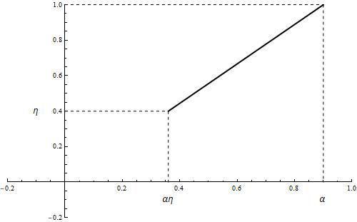
Figure 3. Multifractal spectrum in the case $\alpha=0.9$ and $\eta=0.4$

The paper is organized as follows. Preliminary results are given in Sections 3 and 4. A key point will be to estimate for $j\in\mathbb{N}$, the maximal number of integers $n\in\mathbb{N}^{*}$ satisfying $2^{j}\leq B_{n}^{\frac{1}{\eta}}<2^{j+1}$, such that the support of $\psi_{n}$ contains a given point $x\in[0,1]$ (a bound uniform in $x\in[0,1]$ is obtained). More specifically, we will focus on the so-called ”isolated” pulses $\psi_{n}$, i.e. those pulses whose support intersect only a few number of supports of other pulses with comparable support size. These random covering questions are dealt with in Section 4. This is key to obtain lower and upper estimates for the pointwise Hölder exponents of $F$ at all points and to get Theorem 2.1. More precisely, in Section 5, item (i) of Theorem 2.2 is proved, and a uniform lower bound for all the pointwise Hölder exponents of $F$ is obtained. In Sections 6 and Section 7, we relate the approximation rate of a point $x\in[0,1]$ by some family of random balls to the pointwise regularity of $F$. This allows us to derive the almost sure multifractal spectrum of $F$ in Section 8. In Section 9, we explain how to get the almost everywhere modulus of continuity for $F$ (items (ii) and (iii) of Theorem 2.2). Finally, Section 10 proposes some research perspectives.

3. Preliminary results

Preliminary results are exposed, some of which can be found in standard books [12, 13].

For $j\in\mathbb{N}$, define

$$A_{0} = \{n\in\mathbb{N}^{*}:\ 0\leq B_{n}^{\frac{1}{\eta}}\leq 1\},$$

(6) $$A_{j} = \{n\in\mathbb{N}^{*}:\ 2^{j-1}<B_{n}^{\frac{1}{\eta}}\leq 2^{j}\}\ \ \ \mbox{ when }j>0,$$

$$N_{j} = \mbox{Card}(A_{j}).$$

From its definition, each $N_{j}$ is a Poisson random variable with parameter $2^{\eta j}-2^{\eta(j-1)}$.

Lemma 3.1.

Almost surely, there exist for $j$ large enough,

(7) $$2^{\eta j(1-\varepsilon_{j})}\leq N_{j}\leq 2^{\eta j(1+\varepsilon_{j})}\ \ \mbox{ with }\ \ \varepsilon_{j}=\frac{\log_{2}(j)}{\eta j}.$$

Proof.

Introduce the counting random function $(M_{t})_{t\in\mathbb{R}_{+}^{*}}$ of the point process $(B_{n})_{\mathbb{N}^{*}}$ as $M_{t}=\sup\{n\in\mathbb{N}^{*}\ :\ B_{n}\leq t\}=\sum_{n\in\mathbb{N}^{*}}\mathds{1}_{B_{n}\leq t}$.

For all $0\leq s<t$, $M_{t}-M_{s}$ is a Poisson variable with parameter $(t-s)$. Noting that $N_{j}=M_{2^{\eta j}}-M_{2^{\eta(j-1)}}$, the random variable $N_{j}$ has a Poisson distribution of parameter $a2^{\eta(j-1)}$ where $a=2^{\eta}-1$. By the Bienaymé-Tchebychev inequality, since $\mathbb{E}[N_{j}]=a2^{\eta(j-1)}$, one has

(8) $$\mathbb{P}(|N_{j}-a2^{\eta(j-1)}|\geq j2^{\frac{\eta}{2}(j-1)})\leq\frac{a2^{\eta(j-1)}}{j^{2}2^{\eta(j-1)}}\leq\frac{a}{j^{2}}.$$

By the Borel-Cantelli lemma, a.s. for $j$ large enough, $|N_{j}-a2^{\eta(j-1)}|\leq j2^{\frac{\eta}{2}(j-1)}$. In particular, for every $\alpha>0$ and $j$ large enough, $j^{-\alpha}2^{j\eta}\leq N_{j}\leq j^{\alpha}2^{j\eta}$. This implies (7). ∎

From (8), for every $\alpha>0$, there exists $K>0$ such that for every $j$,

(9) $$\mathbb{P}(N_{j}\notin[2^{\eta j(1-\alpha\varepsilon_{j})},2^{\eta j(1+\alpha\varepsilon_{j})}])\leq\frac{K}{j^{2}}.$$

Observe that (9) indeed holds for every $j$ with a suitable choice for $K$. This will be used later. Bounds for the random variables $B_{n}$ and $C_{n}$ are deduced from the previous results.

Lemma 3.2.

Almost surely, for all $j\in\mathbb{N}$ large enough and $n\in A_{j}$,

(10) $$2^{\eta j(1-\varepsilon_{j})}\leq B_{n},C_{n}\leq 2^{\eta j(1+\varepsilon_{j})}.$$

Proof.

It is standard (from the law of large numbers for instance) that almost surely, for every $n\in\mathbb{N}^{*}$ large enough

(11) $$\frac{n}{2}\leq B_{n}\leq 2n\ \ \mbox{ and }\ \ \frac{n}{2}\leq C_{n}\leq 2n.$$

Let $J\in\mathbb{N}$ be large enough so that (7) holds for $j\geq J$. Call $A=\sum_{j^{\prime}=0}^{J}N_{j^{\prime}}$.

Let $j\geq J+1$, and $n\in A_{j}$. By definition, one has $\sum_{j^{\prime}=0}^{j-1}N_{j^{\prime}}\leq n\leq\sum_{j^{\prime}=0}^{j}N_{j^{\prime}}$.

We apply by (8) with $\alpha=1/2$. On one side,

$$\sum_{j^{\prime}=0}^{j-1}N_{j^{\prime}}\geq N_{j-1}\geq 2^{\eta(j-1)(1-\alpha\varepsilon_{j-1})}\geq K_{1}2^{\eta j(1-\alpha\varepsilon_{j})}\geq 2^{\eta j(1-\varepsilon_{j})}.$$

On the other side, since $j\varepsilon_{j}$ is increasing with $j$, when $j$ becomes large one has

$$\sum_{j^{\prime}=0}^{j}N_{j^{\prime}}\leq A+\sum_{j^{\prime}=J+1}^{j}2^{\eta j^{\prime}(1+\alpha\varepsilon_{j^{\prime}})}\leq A+2^{\eta j\varepsilon_{j}}\sum_{j^{\prime}=J+1}^{j}2^{\eta j^{\prime}}\leq K_{2}2^{\eta j(1+\alpha\varepsilon_{j})},$$

since $A$ is finite. The last term is less than $2^{\eta j(1+\varepsilon_{j})}$, so combining this with (11) gives (10). ∎

Finally, for all $j\in\mathbb{N}$ and $n\in A_{j}$, additional information on the number of pulses $\psi_{n}$ for $n\in A_{j}$ (see (4)) whose support contains a given $x\in[0,1]$ is needed. So, for $x\in[0,1]$, $r>0$ and $n\in\mathbb{N}^{*}$, set

$$T_{n}(x,r)=\left\{\begin{array}[]{ll}1&\mbox{ if }B(X_{n},B_{n}^{-\frac{1}{\eta}})\bigcap B(x,r)\neq\emptyset,\\ 0&\mbox{ otherwise.}\end{array}\right.$$

Next Lemma describes the number of overlaps between the balls $B(X_{n},B_{n}^{-\frac{1}{\eta}})$ for $n\in A_{j}$. It is an improvement of some properties proved in [19].

Lemma 3.3.

Almost surely, there exists $K>0$ such that for every $x\in[0,1]$, for every $J,j\in\mathbb{N}$,

(12) $$\sum_{n\in A_{j}}T_{n}(x,2^{-\eta J})\leq Kj^{2}\max(1,2^{\eta(j-J)}).$$

Proof.

We first work on the dyadic grid. Let $j\in\mathbb{N}$ and $j_{\eta}=\lfloor\eta j\rfloor$. Observe that $[0,1]=\bigcup_{k=0}^{2^{j_{\eta}}-1}I_{j_{\eta},k}$, where $I_{j_{\eta},k}=[k2^{-j_{\eta}},(k+1)2^{-j_{\eta}}].$ For $k\in\{0,1,...,2^{j_{\eta}}-1\}$, and set

(13) $$L_{j,k}=\mbox{Card}\left\{n\in A_{j}\ :\ X_{n}\in I_{j_{\eta},k}\pm 2^{-j_{\eta}+1}\right\}.$$

Let us estimate $p_{j}=\mathbb{P}(\exists k\in\{0,1,...,2^{j_{\eta}}-1\}:L_{j,k}>j^{2}).$ Using Bayes’formula,

$$p_{j} = \mathbb{P}(\exists k\in\{0,1,...,2^{j_{\eta}}-1\},\ L_{j,k}>j^{2}|N_{j}\in[2^{\eta j(1-\varepsilon_{j})},2^{\eta j(1+\varepsilon_{j})}])$$

$$\times\mathbb{P}(N_{j}\in[2^{\eta j(1-\varepsilon_{j})},2^{\eta j(1+\varepsilon_{j})}])$$

$$+\ \ \ \mathbb{P}(\exists k\in\{0,1,...,2^{j_{\eta}}-1\},L_{j,k}>j^{2}|N_{j}\notin[2^{\eta j(1-\varepsilon_{j})},2^{\eta j(1+\varepsilon_{j})}])$$

$$\times\mathbb{P}(N_{j}\notin[2^{\eta j(1-\varepsilon_{j})},2^{\eta j(1+\varepsilon_{j})}]).$$

Applying (9), there exists $K>0$ such that for every $j$,

(14) $$p_{j}\leq\sum_{N\in\{\lfloor 2^{\eta j(1-\varepsilon_{j})}\rfloor,...,\lfloor 2^{\eta j(1+\varepsilon_{j})}\rfloor\}}p_{j,N}\mathbb{P}(N_{j}=N)\ +\frac{K}{j^{2}},$$

where for every integer $N$, $p_{j,N}=\mathbb{P}(\exists k\in\{0,1,...,2^{j_{\eta}}-1\}:L_{j,k}>j^{2}|N_{j}=N).$ Obviously, $p_{j,N}$ is increasing with $N$, hence $p_{j}\leq p_{j,2^{\lfloor\eta j(1+\varepsilon_{j})\rfloor}}+\frac{K}{j^{2}}$.

Conditioned on $N_{j}=n_{0}:=2^{\lfloor\eta j(1+\varepsilon_{j}\rfloor)}$, the law of each $L_{j,k}$ is binomial $B(n_{0},p)$ with parameters $n_{0}$ and $p=\mathbb{P}(X_{n}\in I_{j_{\eta},k}\pm 2^{-j_{\eta}+1})$.

Recall the argument by Demichel and Tricot used in Lemma 2.1 of [Demichel and Tricot(2006)]: For $Y\sim B(n_{0},p)$, then for every $m\geq 1$,

$$\mathbb{P}(Y>m)\leq\frac{(n_{0}p)^{m}}{m!}.$$

In particular, in our case, since $p\leq 3\cdot 2^{-j_{\eta}}\leq 6\cdot 2^{-\eta j}$, one has

$$\mathbb{P}(L_{j,k}>j^{2}|N_{j}=n_{0})\leq\frac{(n_{0}p)^{j^{2}}}{(j^{2})!}\leq\frac{(6\cdot 2^{\eta j(1+\varepsilon_{j})-\eta j})^{j^{2}}}{(j^{2})!}=\frac{(6\cdot j)^{j^{2}}}{(j^{2})!}$$

Hence,

$$p_{j,\lfloor 2^{\eta j(1+\varepsilon_{j})}\rfloor}\leq\sum_{k=0}^{2^{j_{\eta}-1}}\frac{(6\cdot j)^{j^{2}}}{(j^{2})!}\leq\frac{2^{j_{\eta}}(6\cdot j)^{j^{2}}}{(j^{2})!}.$$

Recallng (14), one concludes that

$$p_{j}\leq\frac{2^{j_{\eta}}(6\cdot j)^{j^{2}}}{(j^{2})!}+\frac{K}{j^{2}}$$

which is the general term of a convergent series.

Borel-Cantelli lemma gives that almost surely, for all $j\in\mathbb{N}$ large enough and for every $k\in\{0,1,..,2^{j_{\eta}}-1\}$, $L_{j,k}\leq j^{2}$. So, almost surely, there exists $K>0$ such that for every $j\geq 1$, for every $k\in\{0,1,..,2^{j_{\eta}}-1\}$, $L_{j,k}\leq Kj^{2}$.

To conclude now, fix an integer $J$, $x\in[0,1]$ and $2^{-J-1}\leq r\leq 2^{-J}$. Two cases are distinguished:

• When $j\leq J$: calling again $j_{\eta}=\lfloor j\eta\rfloor$, the point $x$ belongs to a unique interval $I_{j_{\eta},k_{x}}$ (for some unique integer $k_{x}$). When $n\in A_{j}$, observe that $T_{n}(x,2^{-\eta J})=1$ if and only if $|X_{n}-x|\leq 2^{-\eta J}+B_{n}^{-1/\eta}\leq 2^{-\eta J}+2^{-j}$. This may occur only when $X_{n}\in I_{j_{\eta},k_{x}}\pm(2^{-\eta J}+2^{-j})\subset I_{j_{\eta},k_{x}}\pm 2\cdot 2^{-j_{\eta}}$, since $j\leq J$.

  From the consideration above, there are at most $Kj^{2}$ points $X_{n}$, $n\in A_{j}$, such that $T_{n}(x,2^{-\eta J})=1$, hence (12).

• When $j>J$: As above, when $n\in A_{j}$, $T_{n}(x,2^{-\eta J})=1$ may occur only if $|X_{n}-x|\leq 2^{-\eta J}+B_{n}^{-1/\eta}\leq 2^{-\eta J}+2^{-j}\leq 2^{-\lfloor\eta J\rfloor+1}$. The interval $[x-2^{-\lfloor\eta J\rfloor+1},x+2^{-\lfloor\eta J\rfloor+1}]$ is covered by at most $\lfloor 2^{\eta(j-J)+3}\lfloor$ intervals $I_{\lfloor j\eta\rfloor,k}$, and each of these intervals contain at most $Kj^{2}$ points $X_{n}$. So, $T_{n}(x,2^{-\eta J})=1$ for at most $Kj^{2}2^{\eta(j-J)+3}2$ integers $n\in A_{j}$. Hence the result (12).

∎

Observe that the degenerate case $J=+\infty$ also holds in this case, i.e. almost surely, there exists $K>0$ such that for every $x\in[0,1]$, for every $j\in\mathbb{N}$, one has

(15) $$\sum_{n\in A_{j}}T_{n}(x)=\sum_{n\in A_{j}}T_{n}(x,0)\leq Kj^{2}.$$

4. Distribution of isolated pulses

There may be several pulses $\psi_{n}$ with $n\in A_{j}$ whose support intersect each other, creating unfortunate irregularity compensation phenomena and making the estimation of local increments of the process $F$ difficult. In order to circumvent this issue, the knowledge on the distribution of the $\psi_{n}$’s shall be improved.

For this, fix $\gamma\in[1,1/\eta]$ and $p_{0}\in\mathbb{N}$ so large that

(16) $$p_{0}>\frac{3+3\alpha}{1-\alpha\eta}.$$

Let us introduce for any $j\in\mathbb{N}$ the sets

(17) $$\widetilde{A}_{j}=\bigcup_{j^{\prime}=\lfloor(1-p\eta\varepsilon_{j})j\rfloor}^{\lfloor\gamma j\rfloor}A_{j^{\prime}}\ \ \ \mbox{ and }\ \ \ \widetilde{N}_{j}=\mbox{Card}(\widetilde{A}_{j})$$

(18) $$\mathcal{I}_{j}=\{n\in A_{j}\ :\ \forall m\in\widetilde{A}_{j},\ n\neq m,\ B(X_{n},B_{n}^{-\frac{1}{\eta}})\cap B(X_{m},B_{m}^{-\frac{1}{\eta}})=\varnothing\}$$

The elements of $\mathcal{I}_{j}$ are integers $n\in A_{j}$ such that the support of $\psi_{n}$ does not intersect any support of $\psi_{m}$ for $m\in\widetilde{A}_{j}$ with $m\neq n$.

Definition 4.1.

A point $X_{n}$ with $n\in\mathcal{I}_{j}$ is called an isolated point.

The distribution of the isolated points $\{X_{n}\}_{n\in\mathcal{I}_{j}}$ is further investigated. Indeed, as said above, such information is key to obtain upper and lower bounds for the Hölder exponent of $F$ at any point $x$ (see Sections 6 and 7). To describe the distribution of $\{X_{n}\}_{n\in\mathcal{I}_{j}}$, consider the two limsup sets

(19) $$G_{\delta} = \limsup_{j\rightarrow+\infty}\bigcup_{n\in A_{j}}B(X_{n},B_{n}^{-\delta})$$

(20) $$G^{\prime}_{\delta} = \limsup_{j\rightarrow+\infty}\bigcup_{n\in\mathcal{I}_{j}}B(X_{n},B_{n}^{-\delta(1-\widetilde{\varepsilon}_{j})}),\ \ \mbox{ where $\widetilde{\varepsilon}_{j}=\log_{2}(16j\log_{2}j)/(\eta j)$. }$$

Remark 3.

Note that as soon as $\delta>\delta^{\prime}$, $G_{\delta}\subset G_{\delta^{\prime}}$ and $G^{\prime}_{\delta}\subset G^{\prime}_{\delta^{\prime}}$.

In the next sections, it is proved that $G_{\delta}$ contains points whose pointwise Hölder exponent of $F$ is lower-bounded by $\alpha/\delta$ and $G^{\prime}_{\delta}$ points whose pointwise Hölder exponent of $F$ is upper-bounded by $\alpha/\delta$. The idea is that on the support of an isolated pulse, the process $F$ has large local oscillations, thus forming points around which $F$ possesses a low regularity.

Figure 4. Representation of pulses supports in $\mathcal{I}_{j}$.

It is a classical result (see [5, 33]) that almost surely,

(21) $$[0,1]=\limsup_{j\rightarrow+\infty}\bigcup_{n\in A_{j}}B(X_{n},B_{n}^{-(1-\widetilde{\varepsilon}_{j})}).$$

Hence, almost surely, every $x\in[0,1]$ is infinitely many times at distance less than $B_{n}^{-\eta(1-\widetilde{\varepsilon}_{j})}$ from a point $X_{n}$.

A more subtle covering theorem is needed, using only isolated points $(X_{n})_{n\in\mathcal{I}_{j}}$ (instead of $(X_{n})_{n\in A_{j}}$).

Theorem 4.1.

With probability one, $G^{\prime}_{1}=[0,1]$.

Proof.

For $j\in\mathbb{N}$, define the following set

$$D_{j}=\{[8k2^{-\lfloor\eta j\rfloor},(8k+1)2^{-\lfloor\eta j\rfloor}]\ :\ 0\leq 8k<2^{\lfloor\eta j\rfloor}-1\}.$$

Obviously, $\mbox{Card}(D_{j})\sim 2^{\lfloor\eta j\rfloor}/8$.

For all $V\in D_{j}$ (necessarily, $V\subset[0,1]$), consider the following event:

(22) $$\ \ \ \ \ \mathcal{A}_{j}(V)$$

$$=\left\{\exists\,n\in A_{j}\ \mbox{ such that }X_{n}\in V\ \mbox{ and }\ B(X_{n},2B_{n}^{-1-\gamma})\bigcap\bigcup_{m\in\widetilde{A}_{j}}\{X_{m}\}=\{X_{n}\}\right\}$$

Lemma 4.2.

If $\mathcal{A}_{j}(V)$ is realized, then a point $X_{n}$ given by (22) is isolated in the sense of Definition 4.1.

Proof.

When $\mathcal{A}_{j}(V)$ is realized, the point $X_{n}$ is such that for every $m\in\widetilde{A}^{j}$, $X_{m}\notin B(X_{n},2B_{n}^{-1-\gamma})$.

Further, recall that $2^{(j-1)\eta}\leq B_{n}\leq 2^{-j\eta}$, and that $B_{n}^{-1/\eta}<B_{n}^{-1-\gamma}$ by our choice for $\gamma$. In addition, observe that when $m\in\widetilde{A}_{j}$ for $j$ sufficiently large,

$$B_{m}^{-1/\eta} \leq 2^{-(\lfloor(1-p\eta\varepsilon_{j})j\rfloor-1)/\eta}\leq j^{p\eta}2^{-j/\eta+1/\eta}\leq B_{n}^{-1-\gamma},$$

again due to our choice for $\gamma$.

What precedes proves that $B(X_{n},B_{n}^{-1/\eta})\cap B(X_{n},B_{n}^{-1/\eta})=\emptyset$, hence $X_{n}$ is isolated. ∎

Our goal is now to prove that these events $\mathcal{A}_{j}(V)$ are realized very frequently.

The restrictions of the point Poisson process $\{(X_{n},B_{n}\}_{n\in\mathbb{N}}$ on $V\times[1,+\infty]$, or equivalently of $\{(X_{n},B_{n}^{-\frac{1}{\eta}})\}_{n\in\mathbb{N}}$ on $V\times[0,1]$, on the dyadic intervals $V\in D_{j}$, are independent. Moreover, the intervals in $D_{j}$ being pairwise distant from at least $2^{1-\eta j}$, and since $B_{n}^{-1-\gamma}\leq B_{n}^{-1}\leq 2^{1-\eta j}$, two balls $B(X_{n},2B_{n}^{-1-\gamma})$ with $X_{n}\in V$ and $B(X_{m},B_{m}^{-1-\gamma})$ with $X_{m}\in V^{\prime}\neq V$ (with $n,m\in A_{j}$) do not intersect. As a conclusion, the events $\mathcal{A}_{j}(V)$ for $V\in D_{j}$ are independent.

We introduce the set of (random) intervals

$$Q_{j}=\{V\in D_{j}\ :\ \mathcal{A}_{j}(V)\mbox{ is true }\}.$$

Let $V\in D_{j}$ with $V\subset[0,1]$, and consider the random variable $T_{j}(V)=\mathds{1}_{\mathcal{A}_{j}(V)}$. From the above considerations, the random variables $(T_{j}(V))_{V\in D_{j}}$ are i.i.d. random Bernoulli variables with common parameter $p_{j}(1+\gamma)=\mathbb{P}(\mathcal{A}_{j}(V)\ \mbox{ is true})$. Since $\mbox{Card}(Q_{j})=\sum_{V\in D_{j}}T_{j}(V)$, $\sum_{V\in D_{j}}T_{j}(V)\sim\mathcal{B}(\mbox{Card}(D_{j}),p_{j}(1+\gamma))$, a binomial law with parameters $\mbox{Card}(D_{j})$ and $p_{j}(1+\gamma)$.

The parameter is denoted $p_{j}(1+\gamma)$ because, the law of the random variables $X_{n}$ and $B_{n}$ being given, it depends only on $\gamma$ and $j$. To go further, we call for the following lemma that is proved in [5], Lemma 28 (see also [8]).

Lemma 4.3.

There exists a continuous function $k:(1,+\infty)\rightarrow]0,1[$ such that for any $j\in\mathbb{N}^{*}$, $p_{j}(\delta)\geq k(\delta)>0$.

Let $(j_{p})_{p\in\mathbb{N}^{*}}$ be the increasing sequence of integers defined iteratively by $j_{1}=1+\lfloor p\eta\varepsilon_{1}\rfloor$ and $j_{p+1}=\lfloor 2(1/\eta+1)j_{p}+1\rfloor$. By construction, $\widetilde{A}_{j_{p}}\cap\widetilde{A}_{j_{p+1}}=\varnothing$.

Two intervals $V$, $V^{\prime}\in D_{j}$ are called successive when writing $V=[8k2^{-\lfloor\eta j\rfloor},(8k+1)2^{-\lfloor\eta j\rfloor}]$, then either $V^{\prime}=[8(k+1)2^{-\lfloor\eta j\rfloor},(8(2+\gamma)+1)2^{-\lfloor\eta j\rfloor}]$ or $V^{\prime}=[8(k-1)2^{-\lfloor\eta j\rfloor},8k2^{-\lfloor\eta j\rfloor}]$.

Next lemma shows that it is highly likely that amongst any set of $j_{p}\log j_{p}$ successive intervals in $D_{j}$, at least one of them, say $V$, satisfies $\mathcal{A}_{j}(V)$.

Lemma 4.4.

For all $p\in\mathbb{N}$, define the events $\mathcal{E}_{p}$ by

$$\mathcal{E}_{p} = \{\mbox{for all }(V_{1},...,V_{\lfloor j_{p}\log j_{p}\rfloor})\mbox{ successive intervals of }{D}_{j_{p}}$$

$$\ \exists k\in\{1,...,\lfloor j_{p}\log j_{p}\rfloor\}\ \mbox{ such that }\mathcal{A}_{j_{p}}(V_{k})\ \mbox{ is true}\},$$

Then $\mathbb{P}(\limsup\limits_{p\rightarrow+\infty}\mathcal{E}_{p})=1$.

Proof.

It is easily checked that the $\{\mathcal{E}_{p}\}_{p\in\mathbb{N}}$ are mutually independent by our choice for $(j_{p})_{p\geq 1}$. There is a constant $K>0$ such that

$$\mathbb{P}(\mathcal{E}^{c}_{p}) \leq \sum_{i=1}^{\mbox{Card}(D_{j_{n}})}\prod_{k=1}^{\lfloor j_{n}\log j_{n}\rfloor}\mathbb{P}(\mathcal{A}_{j_{n}}(V_{k})\mbox{ is false})$$

$$\leq K2^{\eta j_{p}}(1-p_{j}(1+\gamma))^{j_{p}\log j_{p}}$$

$$\leq K2^{\eta j_{p}}(1-k(1+\gamma))^{j_{p}\log j_{p}}.$$

By construction, $j_{p}>\!\!\!>p$ and $0<1-k(1+\gamma)<1$. This implies that for $p$ large enough, there exists $K^{\prime}>0$ such that $\mathbb{P}(\mathcal{E}^{c}_{p})\leq K^{\prime}e^{-p}$, and so $\mathbb{P}(\mathcal{E}_{p})\geq 1-K^{\prime}e^{-p}$.

In particular, $\sum\limits_{p\in\mathbb{N}}\mathbb{P}(\mathcal{E}_{p})=+\infty$, and Borel-Cantelli’s lemma yields the result. ∎

Let $p$ be such that $\mathcal{E}_{p}$ is realized (this happens for an infinite number of $p$’s).

Soit $V\in D_{j_{p}}$ such that $A_{j}(V)$ holds true. Hence $V$ contains an isolated point, by Lemma 4.2.

From the $\mathcal{E}_{p}$’s and Lemma 4.4, it follows that amongst any $\lfloor{j_{p}}\log{j_{p}}\rfloor$ consecutive intervals in $D_{j_{p}}$ there is at least one interval that contains an isolated point. Consequently,

$$\bigcup\limits_{n\in\mathcal{I}_{j_{p}}}B(X_{n},8j_{p}\log{j_{p}}2^{-\eta{j_{p}}})$$

forms a covering of $[0,1]$. Since this occurs for an infinite number of integers ${j_{p}}$, and recalling (20) and the definition of $\widetilde{\varepsilon}_{j}$, we conclude that almost surely,

$$[0,1]=\limsup\limits_{j\rightarrow+\infty}\bigcup\limits_{n\in\mathcal{I}_{j}}B(X_{n},8j\log{j}2^{-\eta j})\subset\limsup_{j\rightarrow+\infty}\bigcup_{n\in\mathcal{I}_{j}}B(X_{n},B_{n}^{-(1-\widetilde{\varepsilon}_{j})})=G^{\prime}_{1},$$

since $B_{n}\geq 2^{(j_{p}-1)/\eta}$ when $n\in\mathcal{I}_{j_{p}}$. Hence the result. ∎

5. Uniform regularity

In this section, the uniform Hölder regularity of $F$ is investigated.

Recall that $\alpha\in]0,1[$ and $\psi$ is Lipschitz.

An important tool for the following proofs is the wavelet transform. It is known since Jaffard’s works that wavelets provide a convenient method to analyse pointwise regularity of functions.

Definition 5.1.

Let $\phi:\mathbb{R}\to\mathbb{R}$ be a compactly supported, non-zero function, with a vanishing integral: $\displaystyle\int_{\mathbb{R}}\phi(u)du=0$.

The continuous wavelet transform associated with $\phi$ of a function $f\in L^{2}(\mathbb{R})$ is defined for every couple $(s,t)\in\mathbb{R}_{+}^{*}\times\mathbb{R}$ by

(23) $$W_{f}(s,t)=\frac{1}{\sqrt{s}}\int_{\mathbb{R}}f(x)\phi_{s,t}(x)dx\ \ \mbox{ where }\ \ \phi_{s,t}(x)=\phi\left(\frac{x-t}{s}\right).$$

Recall here the theorem of Jaffard [30] and Jaffard-Meyer [36] relating the decay rate of continuous wavelets and uniform regularity for a function $f$.

Theorem 5.1.

Let $H\in\mathbb{R}_{+}^{*}$, $f\in L^{\infty}_{loc}(\mathbb{R})$, and $\psi$ be sufficiently regular (if $\alpha\in]0,1[$ then $\psi$ is a Lipschitz function, otherwise $\psi\in C^{\lfloor\alpha\rfloor+1}(\mathbb{R})$). Then, the mapping $x\mapsto|x|^{H}|\log|x||^{\beta}$ is a uniform modulus of continuity for $f$ if and only if there exists a constant $K>0$ such that

$$\forall(s,t)\in\mathbb{R}_{+}^{*}\times\mathbb{R},\ |W_{f}(s,t)|\leq Ks^{H+\frac{1}{2}}|\log|s||^{\beta}.$$

Next proposition deals with the uniform regularity of $F$.

Proposition 5.2.

Almost surely, for $\alpha\in\mathbb{R}_{+}^{*}\backslash\mathbb{N}$, $\eta\in\mathbb{R}_{+}^{*}$, $\alpha\eta<1$ and $\psi$ sufficiently regular as in Theorem 5.1. Almost surely, there exists $K>0$ such that for any $(s,t)\in[0,1]^{*}\times\mathbb{R}$

$$|W_{F}(s,t)|\leq Ks^{\alpha\eta+\frac{1}{2}}|\log_{2}(s)|^{2+\alpha}.$$

Therefore, item (i) of Theorem 2.2 holds true.

Proof.

Let $(s,t)\in\mathbb{R}_{+}^{*}\times\mathbb{R}$. Note that the wavelet transform $W_{F}$ of $F$ can be expanded in

$$W_{F}(s,t)=\frac{1}{\sqrt{s}}\int_{\mathbb{R}}F(x)\phi_{s,t}(x)dx=\sum_{n=1}^{+\infty}C_{n}^{-\alpha}d_{n}(s,t)$$

with

(24) $$d_{n}(s,t)=\frac{1}{\sqrt{s}}\int_{\mathbb{R}}\psi_{n}(x)\phi_{s,t}(x)dx.$$

A quick computation allows to bound by above $|d_{n}|$ (see Proposition 2.2.1 [19]).

Lemma 5.3.

There exists $K>0$ such that

(25) $$\forall(s,t)\in[0,1]\times\mathbb{R},\ |d_{n}(s,t)|\leq Ks^{\frac{1}{2}}\min\{sB_{n}^{\frac{1}{\eta}},s^{-1}B_{n}^{-\frac{1}{\eta}}\}T_{n}(t,s).$$

Fix $t\in\mathbb{R}$ and $0<s<1$. there exists a unique $J\in\mathbb{N}$ such that $2^{-\eta J+1}\leq s<2^{-\eta J}$.

When $j\leq\eta J$ and $n\in A_{j}$, one has $\min\{sB_{n}^{\frac{1}{\eta}},s^{-1}B_{n}^{-\frac{1}{\eta}}\}=sB_{n}^{\frac{1}{\eta}}\leq s2^{j}$. Also, by Lemma 3.3, $\sum_{n\in A_{j}}T_{n}(t,2^{-\eta J})\leq Kj^{2}$. So, by Lemma 5.3 and (10), there exists a constant $K_{1}>0$ (whose value can change from line to line, but does not depend on $s$, $t$, $j$ or $J$) such that

$${\sum_{j=0}^{\lfloor\eta J\rfloor}}\sum_{n\in A_{j}}C_{n}^{-\alpha}|d_{n}(s,t)| \leq K_{1}s^{\frac{1}{2}}\sum_{j=0}^{\eta J}2^{-\alpha\eta(1-\varepsilon_{j})j}s2^{j}\sum_{n\in A_{j}}T_{n}(t,s)$$

$$\leq K_{1}s^{\frac{1}{2}}\sum_{j=0}^{\eta J}2^{-\alpha\eta(1-\varepsilon_{j})j}s2^{j}\sum_{n\in A_{j}}T_{n}(t,2^{-\eta J})$$

$$\leq K_{1}s^{\frac{3}{2}}\sum_{j=0}^{\eta J}j^{2+\alpha}2^{(1-\alpha\eta)j}\leq K^{\prime}s^{\frac{3}{2}}(\eta J)^{2+\alpha}2^{(1-\alpha\eta)\eta J}$$

$$\leq K_{1}s^{\alpha\eta+\frac{1}{2}}|\log_{2}(s)|^{2+\alpha}.$$

When $\eta J+1\leq j\leq J$, if $n\in A_{j}$ then $\min\{sB_{n}^{\frac{1}{\eta}},s^{-1}B_{n}^{-\frac{1}{\eta}}\}=s^{-1}B_{n}^{-\frac{1}{\eta}}\leq s^{-1}2^{-j}$ and Lemma 3.3 still gives $\sum_{n\in A_{j}}T_{n}(t,2^{-\eta J})\leq Kj^{2}$. Hence, there exists $K_{2}>0$ such that

$${\sum_{j=\lfloor\eta J\rfloor+1}^{J}}\sum_{n\in A_{j}}C_{n}^{-\alpha}|d_{n}(s,t)| \leq K_{2}s^{\frac{1}{2}}\sum_{j=\eta J+1}^{J}2^{-\alpha\eta(1-\varepsilon_{j})j}s^{-1}2^{-j}\sum_{n\in A_{j}}T_{n}(t,2^{-\eta J})$$

$$\leq K_{2}s^{-\frac{1}{2}}\sum_{j=\eta J+1}^{J}j^{2+\alpha}2^{-(1+\alpha\eta)j}\leq K_{2}s^{-\frac{1}{2}}J^{2+\alpha}2^{-(1+\alpha\eta)\eta J}$$

$$\leq K_{2}s^{\alpha\eta+\frac{1}{2}}|\log_{2}(s)|^{2+\alpha}.$$

Finally, when $j\geq J$, $\min\{sB_{n}^{\frac{1}{\eta}},s^{-1}B_{n}^{-\frac{1}{\eta}}\}\leq s^{-1}2^{-j}$ and Lemma 3.3 yields this time $\sum_{n\in A_{j}}T_{n}(t,2^{-\eta J})\leq Kj^{2}2^{\eta(j-J)}$. Hence, there exists $K_{3}>0$ such that

$$\sum_{j=J}^{+\infty}\sum_{n\in A_{j}}C_{n}^{-\alpha}|d_{n}(s,t)| \leq K_{3}s^{\frac{1}{2}}\sum_{j=J}^{+\infty}2^{-\alpha\eta(1-\varepsilon_{j})j}s^{-1}2^{-j}\sum_{n\in A_{j}}T_{n}(t,2^{-\eta J})$$

$$\leq K_{3}s^{-\frac{1}{2}}\sum_{j=J}^{+\infty}j^{2+\alpha}2^{-(1+\alpha\eta)j}2^{\eta(j-J)}\leq K_{3}s^{-\frac{1}{2}}J^{2+\alpha}2^{-(1+\alpha\eta)J}$$

$$\leq K_{3}s^{\alpha\eta+\frac{1}{2}}|\log_{2}(s)|^{2+\alpha}.$$

The combination of the previous inequalities yields that for some constant $K>0$,

$$|W_{F}(s,t)|\leq Ks^{\alpha\eta+\frac{1}{2}}|\log_{2}(s)|^{2+\alpha}.$$

Theorem 5.1 allows to conclude the proof of Proposition 5.2. ∎

6. Lower-bound for the Hölder exponent of $F$ via the study of $G_{\delta}$

When $\delta\in[1,\frac{1}{\eta}]$, next proposition yields a lower bound for the pointwise Hölder exponent of $F$ at $x_{0}$ when $x_{0}\notin G_{\delta}$.

Proposition 6.1.

Almost surely, for every $\delta\in(1,\frac{1}{\eta})$, for every $x_{0}\notin G_{\delta}$, there exists $K_{x_{0}}>0$ such that for any $x$ close to $x_{0}$,

$$|F(x)-F(x_{0})|\leq K_{x_{0}}|\log_{2}|x-x_{0}|\ |^{2+\alpha}|x-x_{0}|^{\frac{\alpha}{\delta}}.$$

Therefore, $h_{F}(x_{0})\geq\frac{\alpha}{\delta}$.

Proof.

Let $x_{0}\notin G_{\delta}$. For $x$ with $|x-x_{0}|\leq 1$, there exists a unique $j_{0}\in\mathbb{N}$ such that

$$2^{-\eta(j_{0}+1)}\leq|x-x_{0}|<2^{-\eta j_{0}}$$

and call $j_{1}$ the largest positive integer so that $|x-x_{0}|+2^{-j_{1}}\leq 2^{-\delta\eta j_{1}}$. The integer $j_{1}$ exists since $2^{-j\eta\delta j_{1}}$ tends to 0 when $j_{1}\to+\infty$.

Observe that when $j_{0}$ becomes large, $|j_{1}-j_{0}/\delta|\to 0$. So it is assumed that $j_{0}$ is so large that $j_{0}/\delta\leq j_{1}\leq j_{0}/\delta+2$, so that $2^{-j_{0}\eta}\sim 2^{-j_{1}\delta\eta}\sim|x-x_{0}|$. Observe also that this explains the fact that $\delta$ must be less or equal than $1/\eta$.

By definition of $G_{\delta}$, since $x_{0}\notin G_{\delta}$, there exists at most a finite number, say $N_{x_{0}}$, of balls $\{B(X_{n_{k}},B_{n_{k}}^{-\delta})\}_{1\leq k\leq N_{x_{0}}}$ that contain $x_{0}$. Write $\widetilde{j}_{0}$ for the smallest integer $j$ such that $\bigcup_{k=1}^{N_{x_{0}}}\{n_{k}\}\in\bigcup_{j=1}^{\widetilde{j}_{0}}A_{j}$. So it may be assumed that $x$ is so close to $x_{0}$ that for every $j\geq j_{1}/2\delta$, $j\varepsilon_{j}\geq\widetilde{j}_{0}+1$ and for every $n\in A_{j}$ with $j\geq j_{1}$, $|x_{0}-X_{n}|>B_{n}^{-\delta}$.

Recalling that the support of $\psi_{n}$ is the ball $B(X_{n},B_{n}^{-1/\eta})$ and that $\delta\leq 1/\eta$, this implies that $x_{0}$ belongs to the support of at most $N$ pulses $\psi_{n}$ with $n\in A_{j}$ and $j<j_{1}$, and does not belong to any support of $\psi_{n}$, for $n\in A_{j}$ and $j\geq j_{1}$.

Also, when $j\leq j_{1}$ and $n\in A_{j}$, by definition of $j_{1}$, one has $|x-x_{0}|+B_{n}^{-1/\eta}\leq B_{n}^{-\delta}$. Hence $x\in B(X_{n},B_{n}^{-1/\eta})$ would imply that $x_{0}\in B(X_{n},B_{n}^{-\delta})$, which is possible for only $N$ balls. Consequently, $x$ and $x_{0}$ both belong to at most $N$ supports of pulses $\psi_{n}$ with $n\in A_{j}$ and $j\leq j_{1}$.

Let us write $|F(x)-F(x_{0})|\leq S_{1}+S_{2}+S_{3}$ with $F_{j}(x)=\sum_{n\in A_{j}}C_{n}^{-\alpha}\psi_{n}(x)$ and

$$S_{1}=\left|\sum_{j=0}^{j_{1}-1}F_{j}(x)-F_{j}(x_{0})\right|,\ \ \ \ S_{2}=\sum_{j=j_{1}}^{+\infty}|F_{j}(x_{0})|\ \ \mbox{ and }\ \ S_{3}=\sum_{j=j_{1}}^{+\infty}|F_{j}(x)|.$$

We first give an upper-bound for $S_{1}$. By the remarks above, $S_{1}$ contains at most $N_{x_{0}}$ non-zero terms of the form $C_{n_{i}}^{-\alpha}(\psi_{n_{i}}(x)-\psi_{n_{i}}(x_{0}))$ (for integers $n_{1}$, …, $n_{N_{x_{0}}}$), and for each of them, since $\psi$ is Lipschitz with some constant $K>0$, one has

$$C_{n_{i}}^{-\alpha}\left|\psi\left(B_{n_{i}}^{\frac{1}{\eta}}\left(x-X_{n_{i}}\right)\right)-\psi\left(B_{n_{i}}^{\frac{1}{\eta}}\left(x_{0}-X_{n_{i}}\right)\right)\right|\leq C_{n_{i}}^{-\alpha}B_{n_{i}}^{\frac{1}{\eta}}K|x-x_{0}|.$$

By (6), (10) and the definition of $\widetilde{j}_{0}$, if ${n_{i}}\in A_{j}$, then one has for some other constant $K>0$ that

$$C_{n_{i}}^{-\alpha}B_{n_{i}}^{\frac{1}{\eta}}\leq K2^{-\alpha\eta j(1-\varepsilon_{j})}2^{j}\leq K\widetilde{j}_{0}^{\alpha}2^{\widetilde{j}_{0}(1-\alpha\eta)}\leq Kj_{1}^{\alpha}2^{\varepsilon_{j_{1}}j_{1}}=Kj_{1}^{\alpha+1/\eta}.$$

Using that $j_{1}\sim\delta j_{0}\sim\frac{\delta}{\eta}|\log_{2}|x-x_{0}||$, this finally gives for some constant $K_{x_{0}}$ depending on $x_{0}$

(26) $$S_{1} \leq KN_{x_{0}}|x-x_{0}|j_{1}^{\alpha+1/\eta}\leq K_{x_{0}}|x-x_{0}|\cdot|\log_{2}|x-x_{0}|\ |^{\alpha+1/\eta}$$

$$\leq |x-x_{0}|^{\alpha}|\log_{2}|x-x_{0}|\ |^{3+\alpha}.$$

Observe that the last inequality holds when $j_{1}$ tends to $+\infty$, and is quite crude.

By construction, $\psi_{n}(x_{0})=0$ for every $n\in A_{j}$ with $j\geq j_{1}$, so $S_{2}=0$.

Finally, for $S_{3}$, one writes that $|\psi_{n}(x)|\leq||\psi||_{\infty}$, and then

$$S_{3} = \sum_{j=j_{1}}^{+\infty}|F_{j}(x)|\leq K||\psi||_{\infty}\sum_{j=j_{1}}^{+\infty}\sum_{n\in A_{j}}C_{n}^{-\alpha}{\bf 1\!\!\!1}_{\psi_{n}(x)\neq 0}$$

$$\leq K||\psi||_{\infty}\sum_{j=j_{1}}^{+\infty}j^{\alpha}2^{-\alpha\eta j}\sum_{n\in A_{j}}T_{n}(x,0)$$

$$\leq K||\psi||_{\infty}\Big{(}\sum_{j=j_{1}}^{+\infty}j^{\alpha}2^{-\alpha\eta j}j^{2}\Big{)}\leq Kj_{1}^{2+\alpha}2^{-\alpha\eta j_{1}}\leq Kj_{0}^{2+\alpha}2^{-j_{0}\frac{\alpha\eta}{\delta}}$$

(28) $$\leq K|\log_{2}|x-x_{0}|\ |^{2+\alpha}\ |x-y|^{\frac{\alpha}{\delta}}.$$

The result follows from (26) and (6), and by letting $\varepsilon$ tend to zero. ∎

7. Upper-bound for the Hölder exponent of $F$ via the sets $G^{\prime}_{\delta}$

We now find an upper bound for the pointwise Hölder exponent of $F$ at every $x_{0}\in G^{\prime}_{\delta}$, using a wavelet method. Let us recall the theorem of Jaffard [30] relating continuous wavelet transforms and pointwise regularity.

Theorem 7.1.

Let $f\in L^{\infty}_{loc}(\mathbb{R})$, $x_{0}\in\mathbb{R}$ and $H>0$. If $f\in C^{H}(x_{0})$, then there exists $K>0$ and a neighborhood $U$ of $(0^{+},x_{0})$ such that

$$\forall(s,t)\in U\ \ ,\ \ |W_{f}(s,t)|\leq Ks^{\frac{1}{2}}(s+|{x_{0}-t}|)^{H}.$$

This theorem is key to prove next proposition.

Proposition 7.2.

Almost surely, for all $\delta\in\left[1,\frac{1}{\eta}\right]$ and $x_{0}\in G^{\prime}_{\delta}$, $h_{F}(x_{0})\leq\frac{\alpha}{\delta}$.

Proof.

First, without loss of generality, assume in addition that the function $\phi$ used to compute the wavelet transform belongs to $C^{1}(\mathbb{R})$, is exactly supported by the interval $[-1,1]$, and that

(29) $$\int_{-1}^{1}\phi(u)\psi(u)du\neq 0.$$

The existence of such a $\phi$ is a trivial exercise.

Fix $x_{0}\in G^{\prime}_{\delta}$. There exist two increasing sequences of integers $(n_{k})_{k\in\mathbb{N}}$ and $(j_{k})_{k\in\mathbb{N}}$ such that $n_{k}\in\mathcal{I}_{j_{k}}$ and $x_{0}\in B(X_{n_{k}},B_{n_{k}}^{-\delta(1-\widetilde{\varepsilon}_{j_{k}})}).$

Let $k\in\mathbb{N}^{*}$ with $n_{k}\in\mathcal{I}_{j_{k}}$. The values of continuous wavelet transforms $W_{F}(B_{n_{k}}^{-\frac{1}{\eta}},X_{n_{k}})$, are now estimated. Setting $J_{k}=\lfloor(1-p_{0}\eta\varepsilon_{j_{k}})j_{k}\rfloor$ and $\widetilde{J}_{k}=\lfloor(1+\gamma)j_{k}\rfloor$, one writes $W_{F}(B_{n_{k}}^{-\frac{1}{\eta}},X_{n_{k}})=S_{1}+S_{2}+S_{3}$ with

$$S_{1} = \sum_{j=0}^{J_{k}-1}\sum_{n\in A_{j}}C_{n}^{-\alpha}d_{n}(B_{n_{k}}^{-\frac{1}{\eta}},X_{n_{k}}),\ \ \ \ S_{2}=\sum_{j=J_{k}}^{\widetilde{J}_{k}}\sum_{n\in A_{j}}C_{n}^{-\alpha}d_{n}(B_{n_{k}}^{-\frac{1}{\eta}},X_{n_{k}})$$

$$\mbox{ and }\ \ S_{3} = \sum_{j=\widetilde{J}_{k}+1}^{+\infty}\sum_{n\in A_{j}}C_{n}^{-\alpha}d_{n}(B_{n_{k}}^{-\frac{1}{\eta}},X_{n_{k}}).$$

Let us first find a lower bound for $S_{2}$. Recalling the definition (18) of $\mathcal{I}_{j_{k}}$, ${n}_{k}$ is the unique integer in $\widetilde{A}_{j_{k}}$ such that $x_{0}\in B(X_{\widetilde{n}_{k}},B_{\widetilde{n}_{k}}^{-\frac{1}{\eta}})$. Hence, recalling (24), $d_{n}(B_{n_{k}}^{-\frac{1}{\eta}},X_{n_{k}})=0$ when $n\neq n_{k}$ (since the support of $\psi_{n}$ and $\phi_{n_{k}}$ do not intersect) and

$$S_{2}=C_{n_{k}}^{-\alpha}d_{n_{k}}(B_{n_{k}}^{-\frac{1}{\eta}},X_{n_{k}}).$$

An integration by part and a change of variables give

$$d_{n_{k}}(B_{n_{k}}^{-\frac{1}{\eta}},X_{n_{k}})=B_{n_{k}}^{-1/(2\eta)}\int_{-1}^{1}\psi(u)\phi(u)du.$$

Condition (29) implies that for some fixed constant $K_{2}>0$ (depending on $\psi$ and $\phi$ only), for every integer $k$,

(30) $$|S_{2}|\geq K_{2}C_{{n}_{k}}^{-\alpha}B_{n_{k}}^{-\frac{1}{2\eta}}\geq K_{2}B_{n_{k}}^{-\frac{1}{2\eta}}2^{-\alpha\eta(1+\varepsilon_{j_{k}})j_{k}}\geq K_{2}B_{n_{k}}^{-\frac{1}{2\eta}-\alpha(1+\varepsilon_{j_{k}})}.$$

where (18) and (10) have been used.

Next, let us estimate $S_{1}$. By (25), (10) and (6), one has

$$|S_{1}| \leq \sum_{j=0}^{J_{k}-1}\sum_{n\in A_{j}}C_{n}^{-\alpha}|d_{n}(B_{n_{k}}^{-\frac{1}{\eta}},X_{n_{k}})|$$

$$\leq \sum_{j=0}^{J_{k}-1}\sum_{n\in A_{j}}C_{n}^{-\alpha}B_{n_{k}}^{-\frac{1}{2\eta}}\min\{B_{n_{k}}^{-\frac{1}{\eta}}B_{n}^{\frac{1}{\eta}},B_{n_{k}}^{\frac{1}{\eta}}B_{n}^{-\frac{1}{\eta}}\}T_{n}(X_{n_{k}},B_{n_{k}}^{-\frac{1}{\eta}})$$

$$\leq \sum_{j=0}^{J_{k}-1}2^{-\alpha\eta j(1-\varepsilon_{j})}B_{n_{k}}^{-\frac{1}{2\eta}}\min\{B_{n_{k}}^{-\frac{1}{\eta}}2^{j},B_{n_{k}}^{\frac{1}{\eta}}2^{-j-1}\}\sum_{n\in A_{j}}T_{n}(X_{n_{k}},2^{-j_{k}}).$$

When $j<(1-\eta\varepsilon_{j_{k}})j_{k}$, $B_{n_{k}}^{-\frac{1}{\eta}}\leq 2^{-j-1}$, so the minimum above is less than $2B_{n_{k}}^{-\frac{1}{\eta}}2^{j}$. In addition, by (7) one has $\sum_{n\in A_{j}}T_{n}(X_{n_{k}},2^{-j_{k}})\leq Kj^{2}$ (this holds as long as $j\leq j_{k}/\eta$). Hence by (12), for some constant $K_{1}>0$ (that may change from one inequality to the next one),

$$|S_{1}| \leq K_{1}\sum_{j=0}^{J_{k}-1}j^{2+\alpha}2^{-\alpha\eta j}B_{n_{k}}^{-\frac{1}{2\eta}}B_{n_{k}}^{-\frac{1}{\eta}}2^{j}\leq K_{1}B_{n_{k}}^{-\frac{3}{2\eta}}\sum_{j=0}^{J_{k}-1}j^{2+\alpha}2^{(1-\alpha\eta)j}$$

$$\leq K_{1}B_{n_{k}}^{-\frac{3}{2\eta}}j_{k}^{2+\alpha}2^{(1-\alpha\eta)(1-p_{0}\eta\varepsilon_{j_{k}})j_{k}}.$$

Since $j_{k}=2^{\eta\varepsilon_{j_{k}}j_{k}}$ and $n_{k}\in\mathcal{I}_{j_{k}}$, $2^{j_{k}}\leq B_{n_{k}}^{\frac{1}{\eta}}$, so

$$|S_{1}| \leq K_{1}B_{n_{k}}^{-\frac{3}{2\eta}}B_{n_{k}}^{(3+\alpha)\varepsilon_{j_{k}}}B_{n_{k}}^{(\frac{1}{\eta}-\alpha)(1-p_{0}\eta\varepsilon_{j_{k}})}\leq K_{1}B_{n_{k}}^{-\frac{1}{2\eta}-\alpha-(p_{0}-3-\alpha-\alpha\eta p_{0})\varepsilon_{j_{k}}}.$$

Our choice (16) for $p_{0}$ ensures that $p_{0}-3-\alpha-\alpha\eta p_{0}>2\alpha$, hence

(31) $$|S_{1}| \leq K_{1}B_{n_{k}}^{-\frac{1}{2\eta}-\alpha(1+2\varepsilon_{j_{k}})}.$$

Finally, for $S_{3}$, one writes by (25), (10) and (6), and the same lines of computations as above, that for some $K_{3}>0$,

$$|S_{3}| \leq \sum_{j=\widetilde{J}_{k}+1}^{+\infty}\sum_{n\in A_{j}}C_{n}^{-\alpha}|d_{n}(B_{n_{k}}^{-\frac{1}{\eta}},X_{n_{k}})|$$

$$\leq K_{3}\sum_{j=\widetilde{J}_{k}+1}^{+\infty}2^{-\alpha\eta j(1-\varepsilon_{j})}B_{n_{k}}^{-\frac{1}{2\eta}}\min\{B_{n_{k}}^{-\frac{1}{\eta}}2^{j},B_{n_{k}}^{\frac{1}{\eta}}2^{-(j+1)}\}\sum_{n\in A_{j}}T_{n}(X_{n_{k}},2^{-j_{k}}).$$

When $j\geq\widetilde{J}_{k}=\lfloor(1+\gamma)j_{k}\rfloor$, the above minimum is now reached at $B_{n_{k}}^{\frac{1}{\eta}}2^{-j-1}$.

Then, still by and (7), the sum $\sum_{n\in A_{j}}T_{n}(X_{n_{k}},2^{-j_{k}})$ is bounded above by $Kj^{2}$ when $j\leq j_{k}/\eta$, and by $Kj^{2}2^{\eta(j-j_{k}/\eta)}$ when $j>j_{k}/\eta$. Hence by (12), for some constant $K_{3}$ that may change from line to line but does not depend on $k$ or any of the moving parameters,

$$|S_{3}| \leq K_{3}\sum_{j=(1+\gamma)j_{k}}^{\lfloor j_{k}/\eta\rfloor}j^{2+\alpha}2^{-\alpha\eta j}B_{n_{k}}^{-\frac{1}{2\eta}}B_{n_{k}}^{\frac{1}{\eta}}2^{-j}$$

$$\ \ \ +K_{3}\sum_{j={\lfloor j_{k}/\eta\rfloor}+1}^{+\infty}j^{2+\alpha}2^{-\alpha\eta j}B_{n_{k}}^{-\frac{1}{2\eta}}B_{n_{k}}^{\frac{1}{\eta}}2^{-j}2^{\eta(j-j_{k}/\eta)}$$

$$\leq K_{3}B_{n_{k}}^{\frac{1}{2\eta}}\left(\sum_{j=(1+\gamma)j_{k}}^{\lfloor j_{k}/\eta\rfloor}j^{2+\alpha}2^{-(1+\alpha\eta)j}+2^{-j_{k}}\sum_{j=\lfloor j_{k}/\eta\rfloor+1}^{+\infty}j^{2+\alpha}2^{(\eta-1-\alpha\eta)j}\right).$$

The first sum above is bounded above by

$$\sum_{j=\lfloor(1+\gamma)j_{k}\rfloor}^{\lfloor j_{k}/\eta\rfloor}j^{2+\alpha}2^{-(1+\alpha\eta)j}\leq K_{3}{j}_{k}^{2+\alpha}2^{-(1+\alpha\eta)(1+\gamma)j_{k}}$$

and the second one by

$$2^{-j_{k}}\sum_{j=\lfloor j_{k}/\eta\rfloor+1}^{+\infty}j^{2+\alpha}2^{(\eta-1-\alpha\eta)j} \leq K_{3}2^{-j_{k}}j_{k}^{2+\alpha}2^{(\eta-1-\alpha\eta)j_{k}/\eta}=K_{3}j_{k}^{2+\alpha}2^{-\frac{j_{k}}{\eta}(1+\alpha\eta)}.$$

Since $B_{n_{k}}^{\frac{1}{\eta}}\sim 2^{j_{k}}$ and $j_{k}=2^{j_{k}\eta\varepsilon_{j_{k}}}\sim B_{n_{k}}^{\varepsilon_{j_{k}}}$ and $1+\gamma<1/\eta$, we get that

$$|S_{3}| \leq K_{3}{j}_{k}^{2+\alpha}2^{-(1+\alpha\eta)(1+\gamma)j_{k}}+K_{3}j_{k}^{2+\alpha}2^{-\frac{j_{k}}{\eta}(1+\alpha\eta)}$$

$$\leq K_{3}B_{n_{k}}^{-\frac{(1+\alpha\eta)(1+\gamma)}{\eta}+(2+\alpha)\varepsilon_{j_{k}}}.$$

Observe that $\frac{(1+\alpha\eta)(1+\gamma)}{\eta}-(2+\alpha)\varepsilon_{j_{k}}>\frac{1}{2\eta}+\alpha(1+2\varepsilon_{j_{k}})$. So,

(33) $$|S_{3}|\leq K_{3}B_{n_{k}}^{-\frac{1}{2\eta}-\alpha(1+2\varepsilon_{j_{k}})},$$

this last inequality being very generous ($S_{3}$ is much smaller than the term on the right hand-side).

Combining (30), (31) and (33), and the fact that $B_{n_{k}}^{-\varepsilon_{j_{k}}}\to 0$ when $k$ tends to infinity, one concludes that for every sufficiently large integers $k$,

(34) $$|W_{F}(B_{n_{k}}^{-\frac{1}{\eta}},X_{n_{k}})|\geq KB_{n_{k}}^{-\frac{1}{2\eta}-\alpha(1+\varepsilon_{j_{k}})}.$$

Assuming that $f\in\mathcal{C}^{\frac{\alpha}{\delta}+\varepsilon}(x_{0})$, we would have by Theorem 7.1 that for some $K^{\prime}>0$,

$$|W_{F}(B_{n_{k}}^{-\frac{1}{\eta}},X_{n_{k}})| \leq K^{\prime}B_{n_{k}}^{-\frac{1}{2\eta}}\Big{(}B_{n_{k}}^{-\frac{1}{\eta}}+|x_{0}-X_{n_{k}}|\Big{)}^{\frac{\alpha}{\delta}+\varepsilon}$$

$$\leq K^{\prime}B_{n_{k}}^{-\frac{1}{2\eta}}\Big{(}B_{n_{k}}^{-\frac{1}{\eta}}+B_{n_{k}}^{-\delta(1-\widetilde{\varepsilon}_{j_{k}})}\Big{)}^{\frac{\alpha}{\delta}+\varepsilon}$$

$$\leq K^{\prime}B_{n_{k}}^{-\frac{1}{2\eta}}B_{n_{k}}^{-\delta(1-\widetilde{\varepsilon}_{j_{k}})(\frac{\alpha}{\delta}+\varepsilon)}$$

since $|x_{0}-X_{n_{k}}|\leq B_{n_{k}}^{-\delta(1-\widetilde{\varepsilon}_{j_{k}})}$. This contradicts (34) since the sequences $(\varepsilon_{j})$ and $(\widetilde{\varepsilon}_{j})$ converge to 0 as $j\to+\infty$. Consequently, $f\notin\mathcal{C}^{\frac{\alpha}{\delta}+\varepsilon}(x_{0})$ for every $\varepsilon>0$, hence the result. ∎

To conclude this part, we would like to emphasize that this analysis is quite sharp since the bounds obtained for $S_{1}$, $S_{2}$ and $S_{3}$ are very tight (and the choice for $p_{0}$ is key). Only the fine study of isolated points made it possible to obtain this result.

Also, observe that the proof does not work any more when $\delta>1/\eta$, since in the last series of inequalities $|W_{F}(B_{n_{k}}^{-\frac{1}{\eta}},X_{n_{k}})|$, the term $B_{n_{k}}^{-\frac{1}{\eta}}+B_{n_{k}}^{-\delta(1-\widetilde{\varepsilon}_{j_{k}})}$ can not be bounded by above by $B_{n_{k}}^{-\delta(1-\widetilde{\varepsilon}_{j_{k}})}$.

8. Multifractal spectrum of $F$

Recall that the study of the regularity of $F$ is restricted to the interval $[0,1]$. We start by the range of possible exponents for $F$.

Lemma 8.1.

Almost surely, for every $x\in[0,1]$, $\alpha\eta\leq h_{F}(x)\leq\alpha$.

Proof.

First, Proposition 5.2 yields that almost surely, for every $x\in[0,1]$, $h_{F}(x)\geq\alpha\eta$.

Then, Theorem 4.1 gives $[0,1]=G^{\prime}_{1}$, and Proposition 7.2 ensures that every $x\in G^{\prime}_{1}$ satisfies $h_{F}(x)\leq\alpha$. ∎

Gathering the results proved in the previous sections (Propositions 6.1 and 7.2, and Remark 3), one also sees that almost surely:

• for all $H\in[\alpha\eta,\alpha)$,

  (35) $$G^{\prime}_{\alpha/H}\setminus\bigcup_{\delta>\frac{\alpha}{H}}G_{\delta}\subset E_{F}(H).$$

  Indeed, when $x\in G^{\prime}_{\frac{\alpha}{H}}$, $h_{F}(x)\leq\frac{\alpha}{\frac{\alpha}{H}}=H$ and when $\delta>\frac{\alpha}{H}$ and $x\notin G_{\delta}$, $h_{F}(x)\geq\frac{\alpha}{\delta}$.

• for all $H\in[\alpha\eta,\alpha]$,

  (36) $$E_{F}(H)\subset\bigcap_{\delta<{\frac{\alpha}{H}}}G_{\delta}.$$

In order to obtain the multifractal spectrum of $F$, a preliminary step consists in estimating the Hausdorff dimension and measures of the sets $G_{\delta}$ and $G^{\prime}_{\delta}$.

For $h>0$, $\mathcal{H}^{h}$, $\mathcal{H}^{h}_{\xi}$ stand respectively for the $h$-Hausdorff measure in $\mathbb{R}$ and the $\alpha$-Hausdorff pre-measure computed with coverings of sets of diameter less than $\xi>0$.

Proposition 8.2.

With probability one, for every $\delta\in[1,1/\eta]$, one has $\dim_{H}G_{\delta}\leq 1/\delta$ and $\mathcal{H}^{1/\delta}(G^{\prime}_{\delta})=+\infty$.

Proof.

The upper bound $\dim_{H}G_{\delta}\leq 1/\delta$ follows by using as coverings of $G_{\delta}$ the family $\{B(X_{n},B^{-\delta}_{n})\}_{j\geq J,n\in A_{j}}$, for $J\geq 1$. For $\varepsilon>0$,

$$\mathcal{H}^{1/\delta+\varepsilon}_{2^{-\eta J}}(G_{\delta}) \leq \sum_{j\geq J}\sum_{n\in A_{j}}|B_{n}^{-\delta}|^{1/\delta+\varepsilon}.$$

By (7), and using that $B_{n}\leq 2^{j\eta}$ when $n\in A_{j}$, one gets

$$\mathcal{H}^{1/\delta+\varepsilon}_{2^{-\eta J}}(G_{\delta})\leq\sum_{j\geq J}2^{\eta j(1+\varepsilon_{j})}2^{-j\eta(1+\varepsilon/\delta)},$$

which is the rest of a convergent series. Hence $\mathcal{H}^{1/\delta+\varepsilon}(G_{\delta})=0$ and $\dim_{H}G_{\delta}\leq 1/\delta+\varepsilon$.

The fact that $\mathcal{H}^{1/\delta}(G^{\prime}_{\delta})=+\infty$ (giving the lower bound $\dim_{H}G^{\prime}_{\delta}\geq 1/\delta$) is more delicate. The following mass transference principle [11, 22] is useful.

Theorem 8.3.

Let $(x_{n})_{n\in\mathbb{N}^{*}}$ be a real sequence in $[0,1]^{d}$ ($d\geq 1$) and $(\lambda_{n})_{n\in\mathbb{N}^{*}}$ a decreasing sequence of positive real numbers. For all $\delta\geq 1$, set

$$L_{\delta}=\limsup_{n\rightarrow+\infty}B(x_{n},\lambda_{n}^{\delta})=\bigcap_{N\geq 1}\bigcup_{n\geq N}B(x_{n},\lambda_{n}^{\delta})$$

If the $d$-dimensional Lebesgue measure $\mathcal{L}(L_{1})$ of $L_{1}$ equals 1, then for all $\delta>1$, $\mathcal{H}^{\frac{d}{\delta}}(L_{\delta})=+\infty$ and $\dim_{\!H}(L_{\delta})\geq\frac{d}{\delta}$.

Theorem 4.1 gives that $G^{\prime}_{1}=[0,1]$, almost surely. In particular, $\mathcal{L}(G^{\prime}_{1})=1$. Applying the previous theorem to the (random) sequences $x_{n}=X_{n}$ and $\lambda_{n}=B_{n}^{-(1-\widetilde{\varepsilon}_{j})}$ when $n\in A_{j}$ yields the claim of Proposition 8.2. ∎

We are now in position to conclude the proof of Theorem 2.1.

Proof.

First, by Lemma 8.1, only $H\in[\alpha\eta,\alpha]$ need to be considered.

Then, (36) yields that almost surely, $d^{[0,1]}_{F}(H)\leq\dim_{\!H}G_{\delta}$, for every $\delta>\alpha/H$. Proposition 8.2 yields $\dim_{\!H}G_{\delta}\leq 1/\delta$, hence $d^{[0,1]}_{F}(H)\leq H/\alpha$.

Finally, Proposition 8.2 gives simultaneously that $\mathcal{H}^{H/\alpha}(G^{\prime}_{\alpha/H})=+\infty$ and $\mathcal{H}^{H/\alpha}(G_{\delta})=0$ for every $\delta<\alpha/H$. So, $\mathcal{H}^{H/\alpha}(G^{\prime}_{\alpha/H}\setminus\bigcup_{\delta>\frac{\alpha}{H}}G_{\delta})=+\infty$, and by (35), $\mathcal{H}^{H/\alpha}(E_{F}(H))=+\infty$. This gives $\dim_{\!H}E_{F}(H)\geq H/\alpha$, and by the remarks above $d^{[0,1]}_{F}(H)=H/\alpha$.

When $H=\alpha$, the same argument gives that $\mathcal{L}(E_{F}(\alpha)\cap[0,1])=1$, i.e. $E_{F}(\alpha)$ is of full Lebesgue measure in $[0,1]$. ∎

9. Almost-everywhere modulus of continuity

Le us explain how to obtain from what precedes the almost-everywhere modulus of continuity for $F$, almost surely.

By a Theorem by Jaffard-Meyer (Proposition 1.2 in [36]), the following (almost) equivalence holds true.

Theorem 9.1.

Let $f\in L^{\infty}_{loc}(\mathbb{R})$, $x_{0}\in\mathbb{R}$ and $H>0$.

If the function $f$ has a local continuity of continuity$\theta$ at $x_{0}$, then for some constant $C>0$

(37) $$\forall(s,t)\in U\ \ ,\ \ |W_{f}(s,t)|\leq Ks^{\frac{1}{2}}(\theta(s)+\theta(|{x_{0}-t}|)).$$

Conversely, if $f\in C^{\varepsilon}(\mathbb{R})$ for some $\varepsilon>0$, and if (37) holds, then there exist constants $\eta,C>0$ and a polynomial $P$ such that setting $j_{0}=\lfloor|\log_{2}|x-x_{0}|\rfloor$, one has

(38) $$\forall x\mbox{ such that }|x-x_{0}|\leq\eta,\ \ |f(x)-P(x-x_{0})|\leq C\inf_{j\geq j_{0}}((j-j_{0})\theta(|x-x_{0}|)+2^{-j\varepsilon}).$$

Observe that if $\theta(h)=|h|^{\beta}|\log|h||^{\gamma}$ with $\varepsilon<\beta<1$, then the infimum at the right hand side of (38) is (roughly) reached at $j=j_{0}\beta/\varepsilon$, and (38) reduces to

$$|f(x)-P(x-x_{0})|\leq C|x-x_{0}|^{\beta}|\log|x-x_{0}||^{1+\gamma}.$$

Coming back to Proposition 7.2, let $x_{0}\in G^{\prime}_{1}$. At the end of the proof, recall the lower bound (34) for the wavelet coefficient $|W_{F}(B_{n_{k}}^{-\frac{1}{\eta}},X_{n_{k}})|\geq KB_{n_{k}}^{-\frac{1}{2\eta}-\alpha(1+\varepsilon_{j_{k}})}$.

Remembering that $B_{n_{k}}\sim 2^{\eta j_{k}}$, the formulas for $\varepsilon_{j_{k}}$ and the fact that $\widetilde{\varepsilon}_{j_{k}}$, and $|x_{0}-X_{n_{k}}|\leq B_{n_{k}}^{-(1-\widetilde{\varepsilon}_{j_{k}})}$, one successively has (for large integers $k$)

$$B_{n_{k}}^{-\varepsilon_{j_{k}}} \sim|\log j_{k}|^{-1}\geq C|\log|x_{0}-X_{n_{k}}||,$$

$$B_{n_{k}}^{-\widetilde{\varepsilon}_{j_{k}}} \sim|\log j_{k}|^{-1}\geq C|\log|x_{0}-X_{n_{k}}||,$$

$$B_{n_{k}}^{-1} \geq C|x_{0}-X_{n_{k}}||\log|x_{0}-X_{n_{k}}||,$$

for some constant $C>0$ that depends on $\eta$ only. Hence,

$$|W_{F}(B_{n_{k}}^{-\frac{1}{\eta}},X_{n_{k}})| \geq KB_{n_{k}}^{-\frac{1}{2\eta}-\alpha(1+\varepsilon_{j_{k}})}\geq KB_{n_{k}}^{-\frac{1}{2\eta}}B_{n_{k}}^{-\alpha}|\log|x_{0}-X_{n_{k}}||^{\alpha}$$

$$\geq KCB_{n_{k}}^{-\frac{1}{2\eta}}|x_{0}-X_{n_{k}}|^{\alpha}|\log|x_{0}-X_{n_{k}}||^{2\alpha}$$

$$\geq\frac{KC}{2}B_{n_{k}}^{-\frac{1}{2\eta}}(\theta(|x_{0}-X_{n_{k}}|)+\theta(B_{n_{k}}^{-\frac{1}{\eta}})),$$

where $\theta(h)=|h|^{\alpha}|\log|h||^{2\alpha}$ and where we used that $B_{n_{k}}^{-\frac{1}{\eta}}<\!\!\!<|x_{0}-X_{n_{k}}|$.

This shows that almost surely, for every $x\in G^{\prime}_{1}$, the modulus of continuity is larger than $|h|^{\alpha}|\log|h||^{2\alpha}$.

Let us now introduce the set

$${\widetilde{G_{1}}}=\limsup_{j\rightarrow+\infty}\bigcup_{n\in A_{j}}B(X_{n},B_{n}^{-(1+3{\varepsilon}_{j})}).$$

Recalling (7), almost surely,

$$\sum_{n\in A_{j}}|B(X_{n},B_{n}^{-(1+2{\varepsilon}_{j})})|\leq 2^{\eta j(1+\varepsilon_{j})}2^{-\eta j(1+3{\varepsilon}_{j})}=j^{-2}.$$

Consequently, ${\widetilde{G_{1}}}$ has zero Lebesgue measure.

Then, a slight adaptation of the proof of Proposition 6.1 shows that almost surely, for every $x_{0}\notin{\widetilde{G_{1}}}$, there exists $K_{x_{0}}>0$ such that for any $x$ close to $x_{0}$,

$$|F(x)-F(x_{0})|\leq K_{x_{0}}|x-x_{0}|^{{\alpha}}|\log_{2}|x-x_{0}|\ |^{3+\alpha}.$$

The modification consists in replacing $\delta$ by $1+3\varepsilon_{j}$, and adapting accordingly the computations.

The conclusion follows by considering the set $G=G^{\prime}_{1}\setminus{\widetilde{G_{1}}}$. Indeed, since $G^{\prime}_{1}$ and ${\widetilde{G_{1}}}$ respectively have full and zero Lebesgue measure, $G$ has full Lebesgue measure. And the two arguments above show that almost surely, for every $x_{0}\in G$, the modulus of continuity $\theta_{x_{0}}$ of $F$ at $x_{0}$ satisfies

$$|h|^{\alpha}|\log|h||^{2\alpha}\leq\theta_{x_{0}}(h)\leq|h|^{{\alpha}}|\log_{2}|h|\ |^{3+\alpha},$$

hence items (ii) and (iii) of Theorem 2.2.

10. Perpectives

The case where $\alpha>1$ is a possible extension of our article.

It is also a natural question for applications to ask whether the sample paths of $F$ satisfy a multifractal formalism.

It would be interesting to determine whether $F$ possess chirps or oscillating singularities, i.e. locally behaves like

$$|x-x_{0}|^{\alpha}|\log|x-x_{0}||^{\beta}$$

around some points $x_{0}$. Chirps are a key notion in many domains - for instance, the existence of gravitational waves has been experimentally proved thanks to wavelet based-algorithms able to detect chirps (that are the signature of coalescent binary black holes) in signals extracted from the LIGO and VIRGO interferometers.

Finally, it is worth investigating the case where the series defining $F$ does not converge uniformly, this may occur for some choices of the parameters $\alpha$ and $\eta$ (recall that in the present paper, the uniform convergence follows from the sparse distribution of the pulses). In this situation, the relevant quantities to analyze are the $p$-exponents of $F$ as defined in [35]: A function $f$ belongs to $T^{p}_{\alpha}(x_{0})$ (which generalizes the spaces $C^{\alpha}(x_{0})$) when there exist a polynomial $P$ and a constant $C>0$ such that

$$\mbox{for every sufficiently small $h>0$, }\ \ \left(\frac{1}{h^{d}}\int_{B(0,h)}|f(x)-P(x)|^{p}\right)^{1/p}\leq C|h|^{\alpha}.$$

Then the $p$-exponent is $h^{p}_{f}(x_{0})=\sup\{\alpha\geq 0:f\in T^{p}_{\alpha}(x_{0})\}$, and the multifractal analysis of the $p$-exponents of $F$ is a challenging issue.

References

- [1] P. Abry, S. Jaffard, S. and H. Wendt, Irregularities and Scaling in Signal and Image Processing: Multifractal Analysis, In Benoit Mandelbrot: A Life in Many Dimensions, M. Frame and N. Cohen, Eds., World scientific publishing, pp 31–116, 2015.
- [2] T.M. Ahsanullah V.B. Nevzorov. Probability Theory. Springer (2015)
- [3] E. Amo, I. Bhouri J. Fernàndez-Sànchez. A note on the Hausdorff dimension of general sums of pulses graphs. Rendiconti del Circolo Matematico di Palermo (2011), 110–123.
- [4] J.-M. Aubry S. Jaffard. Random Wavelet Series. Comm. Math. Phys. (2002), 483–514.
- [5] J. Barral, N. Fournier, S. Jaffard S. Seuret. A pure jump Markov process with a random singularity spectrum. Ann. Proba. (2010), 1924–1946.
- [6] J. Barral B. Mandelbrot. Multifractal products of cylindrical pulses. Probability Theory Related Fields (1985), 125–147.
- [7] J. Barral S; Seuret. Random sparse sampling in a Gibbs weighted tree, J. Inst. Math. Jussieu (2020), 19, no. 1, 65–116.
- [8] J. Barral S. Seuret. A localized Jarnik-Besicovich theorem. Adv. Math. (2011), 3191–3215.
- [9] F. Bayart. Multifractal spectra of typical and prevalent measures. Nonlinearity 26:353–367, 2013.
- [10] M. Ben Abid. Existence and Hölder regularity of pulse functions. Colloquium Mathematicum 116 (2009), 217–225.
- [11] V. Beresnevitch, and S. Velani, A Mass Transference Principle and the Duffin-Schaeffer Conjecture for Hausdorff Measures, Ann. Math., 3 (164), 2006.
- [12] J. Bertoin. Lévy Processes. Cambridge university press (1998).
- [13] L. Breiman. Probability. SIAM (1992).
- [14] Z. Buczolich, J. Nagy. Hölder spectrum of typical monotone continuous functions. Real Anal. Exchange pages 133–156, 1999.
- [15] Z. Buczolich and S. Seuret. Typical Borel measures on [0,1]d satisfy a multifractal formalism. Nonlinearity 23(11):7–13, 2010.
- [16] R. Cioczek-Georges B. Mandelbrot G. Samorodnitsky MS. Taqqu. Stable fractal sums of pulses : the cylindrical case. Bernoulli (1995), 201–216.
- [17] R. Cioczek-Georges B. Mandelbrot. A class of micropulses and antipersistent fractional brownian motion. Stochastic processes and their applications (1995), 1–18.
- [18] R. Cioczek-Georges B. Mandelbrot. Alternative micropulses and fractional brownian motion. Stochastic processes and their applications (1996), 143–152.
- [19] Y. Demichel. Ph.D. Analyse fractale d’une famille de fonctions aléatoire : les fonctions de bosses. Université Blaise Pascal (France) (2006).
- [20] Y. Demichel C. Tricot. Analysis of the Fractal Sum of Pulses. Mathematical Proceedings of the Cambridge Philosophical Society (2006), 355–370.
- [21] Y. Demichel K. Falconer. The Hausdorff dimension of pulse-sum graphs. Mathematical Proceedings of the Cambridge Philosophical Society (2007), 143–145.
- [22] M.M. Dodson, M.V. Melian P. Pestana S.L. Vélani. Patterson measure and Ubiquity. Ann. Acad. Sci. Fenn. Ser. A I Math. (1995), 37–60.
- [23] K. Falconer. Fractal Geométry. Wiley (1990).
- [24] U. Frisch G. Parisi On the singularity structure of fully developed turbulence. Turbulence and predictability in geophysical fluid dynamics and climate dynamics (1974), 84–88.
- [25] Y. Gagne. Ph.D Etude expérimentale de l’intermittence et des singularités dans le plan complexe en turbulence pleinement développée. Université Joseph Fourier (France) (1987).
- [26] C. Bordenave , Y. Gousseau, F. Roueff. The dead leaves model : an example of a general tesselation. Adv. Appl. Probability (2006) 38 (1) pp 31-46.
- [27] P. Calka, Y. Demichel. Fractal random series generated by Poisson-Voronoi tessellations Trans. Amer. Maths. Soc. (2014)
- [Demichel and Tricot(2006)] Y. Demichel and C. Tricot. Analysis of the fractal sum of pulses. Math. Proc. Camb. Phil. Soc., pages 355–370, 2006.
- [28] Y. Heurteaux. Weierstrass functions with random phases Trans. Amer. Math. Soc. (2003), 3065–3077.
- [29] B.R. Hunt. The Hausdorff dimension of graphs of Weierstrass functions. Proc. Amer. Math.Soc. (1998), 781–800.
- [30] S. Jaffard Exposants de Hölder en des points donnés et coefficients d’ondelettes. C.R. Acad. Sci. Paris Sér. I Math. (1989).
- [31] S. Jaffard. The multifractal nature of Lévy processes. Probab. Theory Related Fields, 114(2):207–227, 1999.
- [32] S. Jaffard. On the Frisch-Parisi conjecture. J. Math. Pures Appl. (2000) 79(6):525–552.
- [33] S. Jaffard. On lacunary wavelet series. The Annals of Applied Probability (2000), 313–329.
- [34] S. Jaffard, B. Martin Multifractal analysis of the Brjuno function. Invent. math. 212(2018), 109–132.
- [35] S. Jaffard, C. Melot, R. Leonarduzzi, H. Wendt, P. Abry S. Roux, M. Torres p-exponent and p-leaders, Part I: Negative pointwise regularity. J. (2016), 300–318.
- [36] S. Jaffard Y. Meyer. Wavelet Methods for Pointwise Regularity and Local Oscillations of Functions. AMS (1996).
- [37] J.-P. Kahane. Some Random Series of Function. Cambridge University Press (1985).
- [38] D. Khoshnevisan, Y. Xiao, Y. Zhong Measuring the range of an additive Levy process. Ann. Probab. 31 (2003), 1097–1141.
- [39] S. Lovejoy B. Mandelbrot. Fractal properties of rain, and a fractal model. Tellus (1985), 209–232.
- [40] B. Mandelbrot. Introduction to fractal sums of pulses. Springer (1995), 469–476.
- [41] Y. Pesin. The multifractal analysis of Gibbs measures: Motivation, mathematical foundation, and examples. Chaos 7 (89), 1997.
- [42] F. Roueff. Dimension de Hausdorff du graphe d’une fonction continue: une étude analytique et statistique. PhD thesis, Ecole Nationale Supérieure des Télécommunications (2000).
- [43] L. A. Shepp. Covering the circle with random ares. Israel J. Math. (1972), 328–345.
- [44] N.-R. Shieh, Y. Xiao Hausdorff and packing dimensions of the images of random fields. Bernoulli 16 (2010), 926–952.