Filtering rules for flow time minimization in a Parallel Machine Scheduling Problem

Abstract

This paper studies the scheduling of jobs of different families on parallel machines with qualification constraints. Originating from semi-conductor manufacturing, this constraint imposes a time threshold between the execution of two jobs of the same family. Otherwise, the machine becomes disqualified for this family. The goal is to minimize both the flow time and the number of disqualifications. Recently, an efficient constraint programming model has been proposed. However, when priority is given to the flow time objective, the efficiency of the model can be improved.

This paper uses a polynomial-time algorithm which minimize the flow time for a single machine relaxation where disqualifications are not considered. Using this algorithm one can derived filtering rules on different variables of the model. Experimental results are presented showing the effectiveness of these rules. They improve the competitiveness with the mixed integer linear program of the literature.

keywords : Parallel Machine Scheduling, Job families , Flow time , Machine Disqualification, Filtering Algorithm , Cost-Based Filtering.

1 Introduction

This paper considers the scheduling of job families on parallel machines with time constraints on machine qualifications. In this problem, each job belongs to a family and a family can only be executed on a subset of qualified machines. In addition, machines can lose their qualifications during the schedule. Indeed, if no job of a family is scheduled on a machine during a given amount of time, the machine lose its qualification for this family. The goal is to minimize the sum of job completion times, i.e. the flow time, while maximizing the number of qualifications at the end of the schedule.

This problem, called scheduling Problem with Time Constraints (PTC), is introduced in [11]. It comes from the semiconductor industries. Its goal is to introduce constraints coming from Advanced Process Control (APC) into a scheduling problem. APC’s systems are used to control processes and equipment to reduce variability and increase equipment efficiency. In PTC, qualification constraints and objective come from APC and more precisely from what is called Run to Run control. More details about the industrial problem can be found in [10].

Several solution methods has been defined for PTC [11, 10, 7]. In particular, the authors of [7] present two pre-existing models: a Mixed Integer Linear Program (MILP) and a Constraint Programming (CP) model. Furthermore, they define a new CP model taking advantage of advanced CP features to model machine disqualifications. However, the paper shows that when the priority objective is the flow time, the performance of the CP model can be improved.

The objective of this paper is to improve the performances of the CP model for the flow time objective. To do so, a relaxed version of PTC where qualification constraints are removed is considered. For this relaxation, the results of Mason and Anderson [9] are adapted to define an algorithm to optimally sequence jobs on one machine in polynomial time. This algorithm is then used to define several filtering algorithms for PTC.

Although, the main result of this paper concerns the filtering algorithms for PTC, there is also two more general results incident to this work. First, those algorithms can be directly applied to any problem having a flow time objective and which can be relaxed to a parallel machine scheduling problem with sequence-independent family setup times. Secondly, the approach is related to cost-based domain filtering [3], a general approach to define filtering algorithms for optimization problems.

The paper is organized as follows. Section 2 gives a formal description of the problem the CP model for PTC. Section 3 presents the relaxed problem and the optimal machine flow time computation of the relaxed problem. Section 4 shows how this flow time is used to define filtering rules and algorithms for PTC. Finally, Section 5 shows the performance of the filtering algorithms and compares our results to the literature.

2 Problem description and modeling

In this section, a formal description of PTC is given. Then, a part of the CP model of [7] is presented. The part of the model presented is the part that is useful to present our cost based filtering rules and correspond to the modeling of the relaxation. Indeed, as we are interested in the flow time objective, the machine qualification modeling is not presented in this paper.

2.1 PTC description

Formally, the problem takes as input a set of jobs, ${\cal N}=\{1,\dots,N\}$, a set of families ${\cal F}=\{1,\dots,F\}$ and a set of machines, ${\cal M}=\{1,\dots,M\}$. Each job $j$ belongs to a family and the family associated with $j$ is denoted by $f(j)$. For each family $f$, only a subset of the machines ${\cal M}_{f}\subseteq{\cal M}$, is able to process a job of $f$. A machine $m$ is said to be qualified to process a family $f$ if $m\in{\cal M}_{f}$. Each family $f$ is associated with the following parameters:

• $n_{f}$ denotes the number of jobs in the family. Note that $\sum_{f\in{\cal F}}n_{f}=N$.

• $p_{f}$ corresponds to the processing time of jobs in $f$.

• $s_{f}$ is the setup time required to switch the production from a job belonging to a family $f^{\prime}\neq f$ to the execution of a job of $f$. Note that this setup time is independent of $f^{\prime}$, so it is sequence -independent. In addition, no setup time is required neither between the execution of two jobs of the same family nor at the beginning of the schedule, i.e. at time $0$.

• $\gamma_{f}$ is the threshold value for the time interval between the execution of two jobs of $f$ on the same machine. Note that this time interval is computed on a start-to-start basis, i.e. the threshold is counted from the start of a job of family $f$ to the start of the next job of $f$ on machine $m$. Then, if there is a time interval $]t,t+\gamma_{f}]$ without any job of $f$ on a machine, the machine lose its qualification for $f$.

The objective is to minimize both the sum of job completion times, i.e. the flow time, and the number of qualification looses or disqualifications. An example of PTC together with two feasible solutions is now presented.

Example 1.

Consider the instance with $N=10,\ M=2$ and $F=3$ given in Table 1(a). Figure 1 shows two feasible solutions. The first solution, described by Figure 1(b), is optimal in terms of flow time. For this solution, the flow time is equal to $1+2+9+15+21+1+2+12+21+30=114$ and the number of qualification losses is $3$. Indeed, machine $1$ ($m_{1}$) loses its qualification for $f_{3}$ at time $22$ since there is no job of $f_{3}$ starting in interval $]1,22]$ which is of size $\gamma_{3}=21$. The same goes for $m_{2}$ and $f_{3}$ at time $22$ and for $m_{2}$ and $f_{2}$ at time $26$.
The second solution, described by Figure 1(c), is optimal in terms of number of disqualifications. Indeed, in this solution, none of the machines loses their qualifications. However, the flow time is equal to $1+2+9+17+19+9+18+20+27+37=159$.

$f$	$n_{f}$	$p_{f}$	$s_{f}$	$\gamma_{f}$	${\cal M}_{f}$
1	3	9	1	25	$\{2\}$
2	3	6	1	26	$\{1,2\}$
3	4	1	1	21	$\{1,2\}$

(a) Instance with $N=10,\ M=2$ and $F=3$

(b) An optimal solution for the flow time objective

(c) An optimal solution for qualification losses

Figure 1: Two solution examples for PTC.

2.2 CP model

In the following section, the part of the CP model of [7] which is useful for this work is recalled. This part corresponds to a Parallel Machine Scheduling Problem (PMSP) with family setup times. New auxiliary variables used by our cost based filtering rules are also introduced. These variables are written in bold in the variable description. To model the PMSP with family setup times, (optional) interval variables are used [5, 6]. To each interval variable $J$, a start time $st(J)$, an end time $et(J)$, a duration $d(J)$ and an execution status $x(J)$ is associated. The execution status $x(J)$ is equal to $1$ if and only if $J$ is present in the solution and $0$ otherwise.
The following set of variables is used:

• $jobs_{j},\ \forall j\in{\cal N}$: Interval variable modeling the execution of job $j$;

• $altJ_{j,m},\ \forall(j,m)\in{\cal N}\times{\cal M}_{f(j)}$: Optional interval variable modeling the assignment of job $j$ to machine $m$;

• $\mathbf{flowtime_{m}}$ and $flowtime$: Integer variables modeling respectively the flow time on machine $m$ and the global flow time;

• $\mathbf{nbJobs_{f,m}},\forall(f,m)\in{\cal F}\times{\cal M}_{f}$: Integer variable modeling the number of jobs of family $f$ scheduled on $m$;

• $\mathbf{nbJobs_{m}},\forall m\in{\cal M}$: Integer variable modeling the number of jobs scheduled on $m$.

To model the PMSP with setup time, the following sets of constraints is used:

$$flowTime=\sum_{j\in{\cal N}}et(jobs_{j})$$ (1)

$$alternative\left(jobs_{j},\left\{altJ_{j,m}|m\in{\cal M}_{f(j)}\right\}\right) \forall j\in{\cal N}$$ (2)

$$noOverlap\left(\left\{altJ_{j,m}|\forall j\ s.t.\ m\in{\cal M}_{f(j)}\right\},S\right) \forall m\in{\cal M}$$ (3)

$$flowtime=\sum_{m\in{\cal M}}flowtime_{m}$$ (4)

$$flowtime_{m}=\sum_{j\in{\cal N}}et(altJ_{j,m}) \forall m\in{\cal M}$$ (5)

$$nbJobs_{f,m}=\sum_{j\in{\cal N};f(j)=f}x(altJ_{j,m}) \forall(f,m)\in{\cal F}\times{\cal M}_{f}$$ (6)

$$\sum_{m\in{\cal M}}nbJobs_{f,m}=n_{f} \forall f\in{\cal F}$$ (7)

$$\sum_{f\in{\cal F}}nbJobs_{f,m}=nbJobs_{m} \forall m\in{\cal M}$$ (8)

$$\sum_{m\in{\cal M}}nbJobs_{m}=N$$ (9)

Constraint (1) is used to compute the flow time of the schedule. Constraints (2)–(3) are used to model the PMSP with family setup time. Constraints (2) model the assignment of jobs to machine. Constraints (3) ensure that jobs do not overlap and enforce setup times. Note that $S$ denotes the setup time matrix: $(S_{f,f^{\prime}})$ is equal to $0$ if $f=f^{\prime}$ and to $s_{f}$ otherwise. A complete description of alternative and noOverlap constraints can be found in [5, 6].
In [7], additional constraints are used to make the model stronger, e.g. ordering constraints, cumulative relaxation. They are not presented in this paper.
Constraints (4)–(9) are used to link the new variables to the model. Constraints (4) and (5) ensure machine flow time computation. Constraints (6) compute the number of jobs of family $f$ executed on machine $m$. Constraints (7) make sure the right number of jobs of family $f$ is executed. Constraints (8) and (9) are equivalent to constraints (6) and (7) but for the total number of jobs scheduled on machine $m$. The bi-objective optimization is a lexicographical optimization or its linearization [2].

3 Relaxation description and sequencing

3.1 ${\cal R}$-PTC description

The relaxation of PTC (${\cal R}$-PTC) is a parallel machine scheduling problem with sequence-independent family setup time without the qualification constraints (parameter $\gamma_{f}$). The objective is then to minimize the flow time. In this section, it is assumed that a total the assignment of jobs to machines is already done and the objective is to sequence jobs so the flow time is minimal. Therefore, since the sequencing of jobs on $M$ machines can be seen as $M$ one machine problems, this section presents how jobs can be sequenced optimally on one machine. In Section 4, the cost-based filtering rules handle partial assignments of jobs to the machines.

3.2 Optimal sequencing for ${\cal R}$-PTC

The results presented in this section were first described in [8]. They are adapted from Mason and Anderson [9] who considers an initial setup at the beginning of the schedule. The results are just summarized in this paper.

First, a solution can be represented as a sequence $S$ representing an ordered set of $n$ jobs. Considering job families instead of individual jobs, $S$ can be seen as a series of blocks, where a block is a maximal consecutive sub-sequence of jobs in $S$ from the same family (see Figure 2). Let $B_{i}$ be the $i$-th block of the sequence, $S=\{B_{1},B_{2},\dots,B_{r}\}$. Hence, successive blocks contain jobs from different families. Therefore, there will be a setup time before each block (except the first one).

Figure 2: Block representation of a solution.

The idea of the algorithm is to adapt the Shortest Processing Time ($SPT$) rule [12] for blocks instead of individual jobs. To this end, blocks are considered as individual jobs with processing time $P_{i}=s_{f_{i}}+|B_{i}|\cdot p_{f_{i}}$ and weight $W_{i}=|B_{i}|$ where $f_{i}$ denotes the family of jobs in $B_{i}$ (which is the same for all jobs in $B_{i}$).

The first theorem of this section states that there always exists an optimal solution $S$ containing exactly $|{\cal F}|$ blocks and that each block $B_{i}$ contains all jobs of the family $f_{i}$. That is, all jobs of a family are scheduled consecutively.

Theorem 1.

Let ${\cal I}$ be an instance of the problem. There exists an optimal solution $S^{*}=\{B_{1},\dots,B_{|{\cal F}|}\}$ such that $|B_{i}|=n_{f_{i}}$ where $f_{i}$ is the family of jobs in $B_{i}$.

Sketch.

For a complete proof of the theorem, see [8].
Consider an optimal solution $S=\{B_{1},\dots,B_{u},\dots,B_{v},\dots,B_{r}\}$ with two blocks $B_{u}$ and $B_{v}$ ($u<v$), containing jobs of the same family $f_{u}=f_{v}=f$. Then, moving the first job of $B_{v}$ at the end of block $B_{u}$ can only improve the solution.

Indeed, let us define $P$ and $W$ as: $P=\sum_{i=u+1}^{v-1}P_{i}+s_{f}$ and $W=\sum_{i=u+1}^{v-1}|B_{i}|$. In addition, let $S^{\prime}$ be the sequence formed by moving the first job of $B_{v}$, say job $j_{v}$, at the end of block $B_{u}$. The difference on the flow time between $S$ and $S^{\prime}$, is as follows:

$FT_{S^{\prime}}-FT_{S}=\left\{\begin{array}[]{lcl}W\cdot p_{f}-P&&\text{ if }|B_{v}|=1\\ W\cdot p_{f}-P-\sum_{i=v+1}^{r}|B_{i}|\cdot s_{f}&&\text{ if }|B_{v}|>1\\ \end{array}\right.$

Using Lemma 1 of [8] stating that $P/W\geq p_{f}$, then $FT_{S^{\prime}}-FT_{S}<0$ and the flow time is improved in $S^{\prime}$. Hence, moving the first job of $B_{v}$ at the end of block $B_{u}$ leads to a solution $S^{\prime}$ at least as good as $S$.

Therefore, a block $B_{i}$ contains all jobs of family $f_{i}$. Indeed, if not, applying the previous operation leads to a better solution. Hence, $|B_{i}|=n_{f_{i}}$ and there are exactly $F$ blocks in the optimal solution, i.e. one block per family. ∎

At this point, the number of block and theirs contents are defined. The next step is to order them. To this end, the concept of weighted processing time is also adapted to blocks as follows.

Definition 1.

The Mean Processing Time (MPT) of a block $B_{i}$ is defined as $MPT(B_{i})=P_{i}/W_{i}$.

One may think that, in an optimal solution, jobs are ordered by $SMPT$ (Shortest Mean Processing Time). However, this is not always true since no setup time is required at time $0$. Indeed, the definition of block processing time always considers a setup time before the block. In our case, this is not true for the first block. Example 2 gives a counter-example showing that scheduling all blocks according to the SMPT rule is not optimal.

Example 2 (Counter-example – Figure 3).

Consider the instance given by Table 3(a) that also gives the MPT of each family ($MPT_{f}=p_{f}+(s_{f}\div\ n_{f})$). Figure 3(b) shows the SMPT rule may lead to sub-optimal solutions when no setup time is required at time $0$. Indeed, following the SMPT rule, jobs of family $1$ have to be scheduled before jobs of family $2$. This leads to a flow time of $198$. However, schedule jobs of family $2$ before jobs of family $1$ leads to a better flow time, i.e. $181$.

$f$	$n_{f}$	$p_{f}$	$s_{f}$	$MPT_{f}$
1	2	11	2	12
2	3	12	9	15

(a) Instance with $N=5$ and $F=2$.

(b) Scheduling jobs of a family before those of the other one. Numbers are completion times of the jobs.

Figure 3: Scheduling all blocks according to the SMPT rule is not optimal.

Actually, the only reason why the $SMPT$ rule does not lead to an optimal solution is that no setup time is required at time $0$. Therefore, in an optimal solution, all blocks except the first one are scheduled according to the $SMPT$ rule. That is the statement of Theorem 2 for which a proof is given in [8].

Theorem 2.

In an optimal sequence of the problem, the blocks $2$ to $|{\cal F}|$ are ordered by $SMPT$ (Shortest Mean Processing Time). That is, if $1<i<j$ then $MPT(B_{i})\leq MPT(B_{j})$.

The remaining of this section explains how these results are used to define a polynomial time algorithm for sequencing jobs on a machine so the flow time is minimized. This algorithm is called sequencing in the remaining of the paper.

Theorem 1 states that there exists an optimal solution $S$ containing exactly $|{\cal F}|$ blocks and that each block $B_{i}$ contains all jobs of family $f_{i}$. Theorem 2 states that the blocks $B_{2}$ to $B_{|{\cal F}|}$ are ordered by $SMPT$. Finally, one only needs to determine which family is processed in the very first block.

Algorithm sequencing takes as input the set of jobs and starts by grouping them in blocks and sorting them in SMPT order. The algorithm then computes the flow time of this schedule. Each block is then successively moved to the first position (see Figure 4) and the new flow time is computed. The solution returned by the algorithm is therefore the one achieving the best flow time.

(a) SMPT Sequence

(b) $B_{f}$ is moved in the first position.

Figure 4: SMPT Sequence and Move Operation.

The complexity for ordering the families in $SMPT$ order is $O(F\log{F})$. The complexity of moving each block to the first position and computing the corresponding flow time is $O(F)$. Indeed, there is no need to re-compute the entire flow time. The difference of flow time coming from the Move operation can be computed in $O(1)$. Hence, the complexity of sequencing is $O(F\log{F})$.

4 Filtering rules and algorithms

This section is dedicated to the cost-based filtering rules and algorithms derived from the results of Section 3. They are separated into three parts, each one corresponding to the filtering of one variable: $flowtime_{m}$ (Section 4.1); $nbJobs_{f,m}$ (Section 4.2); $nbJobs_{m}$ (Section 4.3). Note that the two last variables constrained by the sum constraint 8.

During the solving of the problem, jobs are divided for each machine $m$ into three categories based on the interval variables $altJ_{j,m}$: each job either is, or can be, or is not, assigned to the machine. Note that the time windows of the interval variables are not considered in the relaxation. For a machine $m$, let ${\cal N}_{m}^{A}$ be the set of jobs for which the assignment to machine $m$ is decided. In the following of this section, an instance $\cal I$ is always considered with the set ${\cal N}^{A}=\cup_{m\in{\cal M}}{\cal N}_{m}^{A}$ of jobs already assigned to a machine. Thus, an instance is denoted by $({\cal I},{\cal N}^{A})$.

Some notations are now introduced. For a variable $x$, $\underline{x}$ (resp. $\overline{x}$) represents the lower (resp. the upper) bound on the variable $x$. Furthermore, let $FT^{*}({\cal X})$ be the flow time of the solution returned by the algorithm sequencing applied on the set of jobs ${\cal X}$.

4.1 Increasing the machine flow time

The first rule updates the lower bound on the $flowtime_{m}$ variable and follows directly from Section 3. The complexity of this rule is $O(M\cdot F\cdot\log{F})$.

Rule 1.

$\forall m\in{\cal M},\ flowtime_{m}\geq FT^{*}({\cal N}_{m}^{A})$

Proof.

It is sufficient to notice that, for a machine $m$, sequencing gives a lower bound on the flow time. In particular, $FT^{*}({\cal N}_{m}^{A})$ is a lower bound on the flow time of $m$ for the instance $({\cal I},{\cal N}^{A})$. ∎

Example 3.

Consider an instance with $3$ families. Their parameters are given by Table 5(a). A specific machine $m$ is considered and set ${\cal N}_{m}^{A}$ is composed of one job of each family. This instance and ${\cal N}_{m}^{A}$ is used in all the example of this section.
Suppose $flowtime_{m}\in[0,35]$. The output of sequencing is given on the top of Figure 5(b). Thus, the lower bound on the flow time can be updated to $2+7+13=22$, i.e. $flowtime_{m}\in[22,35]$.
Suppose now that an extra job of family $f_{2}$ is added to ${\cal N}_{m}^{A}$ (on the bottom of Figure 5(b)). Thus, $FT^{*}({\cal N}_{m}^{A})=2+8+11+16=37$ and $37>\overline{flowtime}_{m}=35$. Thus, the assignment defined by ${\cal N}_{m}^{A}$ is infeasible.

$f$	$n_{f}$	$p_{f}$	$s_{f}$
1	3	2	5
2	3	3	3
3	4	4	1

(a) Instance data.

(b) Illustration of Rule 1 and Rule 3.

Figure 5: Illustration of $flowtime_{m}$ filtering (Rule 1).

Another rule can be defined to filter $flowtime_{m}$. This rule is stronger than Rule 1 and is based on ${\cal N}_{m}^{A}$ and $\underline{nbJobs}_{m}$. Indeed, $\underline{nbJobs}_{m}$ denotes the minimum number of jobs that has to be assigned to $m$. Thus, if one can find the $\underline{nbJobs}_{m}$ jobs (including the one of ${\cal N}_{m}^{A}$) that leads to the minimum flow time, it will give a lower bound on the flow time of machine $m$.
Actually, it may be difficult to know exactly which jobs will contribute the least to the flow time. However, considering jobs in $SPT$ order and with $0$ setup time gives a valid lower bound on $flowtime_{m}$. First, an example illustrating the filtering rule is presented and then, the rule is formally given.

Example 4.

Consider the instance described in Example 3. Suppose ${\cal N}_{m}^{A}$ is composed of one job of each family and $flowtime_{m}\in[22,60]$. Suppose also $\underline{nbJobs}_{m}=6$. Thus, $3$ extra jobs need to be assigned to $m$.
Families in $SPT$ order are $\{f_{1},f_{2},f_{3}\}$ and the remaining number of jobs in each family is $2,2,3$. Hence, the $3$ extra jobs are: $2$ jobs of $f_{1}$ and $1$ job of $f_{2}$.
To make sure the lower bound on the flow time is valid, those jobs are sequenced on $m$ with no setup time. In Figure 6, $f_{j}$ denotes “classical” jobs of family $f_{j}$ while $f_{j}^{\prime}$ denotes jobs of family $f_{j}$ with no setup time.
Figure 6 shows the results of sequencing on the set of jobs composed of ${\cal N}_{m}^{A}$ plus the $3$ extra jobs, i.e. $\underline{nbJobs}_{m}=6$. Here, $FT^{*}=2+4+6+9+14+20=55$. Thus, the lower bound on $flowtime_{m}$ can be updated and $flowtime_{m}\in[55,60]$.

Figure 6: Illustration of $flowtime_{m}$ filtering (Rule 2).

Note that, because Rule 1 does not take $\underline{nbJobs}_{m}$ into account, it gives a lower bound of $22$ in this case.

Let ${\cal N}_{m}^{O}$ denotes the set composed of the first $\underline{nbJobs}_{m}-|{\cal N}_{m}^{A}|$ remaining jobs in $SPT$ order with setup time equal to $0$.

Rule 2.

$\forall m\in{\cal M},\ flowtime_{m}\geq FT^{*}({\cal N}_{m}^{A}\cup{\cal N}_{m}^{O})$

Proof.

First note that if ${\cal N}_{m}^{O}=\emptyset$, Rule 1 gives the result. Thus, suppose that $|{\cal N}_{m}^{O}|\geq 1$. By contradiction, suppose $\exists m\in{\cal M}$ such that $flowtime_{m}<FT^{*}({\cal N}_{m}^{A}\cup{\cal N}_{m}^{O})$. Thus, there exists another set of jobs $\overline{N_{m}^{O}}$ with:

$$FT^{*}({\cal N}_{m}^{A}\cup\overline{N_{m}^{O}})<FT^{*}({\cal N}_{m}^{A}\cup{\cal N}_{m}^{O})$$ (10)

First, note that w.l.o.g. $|\overline{N_{m}^{O}}|=|{\cal N}_{m}^{O}|$. Indeed, if $|\overline{N_{m}^{O}}|>|{\cal N}_{m}^{O}|$, we can remove jobs from $|\overline{N_{m}^{O}}|$ without increasing the flow time. Furthermore, w.l.o.g. we can consider that $\forall j\in\overline{N_{m}^{O}},\ s_{f_{j}}=0$. Indeed, since setup times can only increase the flow time, thus inequality (10) is still verified.
Let $\overline{S}=\{\overline{j}_{1},\cdots,\overline{j}_{nbJobs_{m}}\}$ be the sequence returned by the sequencing algorithm on ${\cal N}_{m}^{A}\cup\overline{N_{m}^{O}}$. Let also $\overline{j}_{i}$ be the job in $\overline{N_{m}^{O}}\setminus{\cal N}_{m}^{O}$ with the $SPT$. Finally, let $j_{k}$ be the job with the $SPT$ in $\in{\cal N}_{m}^{O}\setminus\overline{N_{m}^{O}}$. Thus, since $p_{f_{\overline{j}_{i}}}>p_{f_{j_{k}}}$, sequence $\overline{S}^{\prime}=\{\overline{j}_{1},\cdots,\overline{j}_{i-1},j_{k},\overline{j}_{i+1},\cdots\overline{j}_{nbJobs_{m}}\}$ has a smaller flow time than $\overline{S}$.

Repeated applications of this operation yield to a contradiction with equation (10). ∎

The complexity of Rule 2 is $O(M\cdot F\cdot\log{F})$. Indeed, sorting families in $SPT$ order can be done in $O(F\cdot log{F})$. Creating the set ${\cal N}_{m}^{O}$ is done in $O(F)$ and sequencing is applied in $O(F\cdot log{F})$ which gives a total complexity of $O(F\cdot log{F}+M\cdot(F+F\cdot\log{F}))$.

4.2 Reducing the maximum number of jobs of a family

The idea of the filtering rule presented in this section is as follows. For a family $f$, $\overline{nbJobs}_{f,m}$ define the maximum number of jobs of family $f$ that can be scheduled on $m$. Thus, if adding those $\overline{nbJobs}_{f,m}$ to ${\cal N}_{m}^{A}$ leads to an infeasibility, $\overline{nbJobs}_{f,m}$ can be decreased by at least $1$. Let denote by ${\cal N}_{m}^{f}$ the set composed of $\overline{nbJobs}_{f,m}$ jobs of family $f$ minus those already present in ${\cal N}_{m}^{A}$.

Rule 3.

If $\exists(f,m)\in{\cal F}\times{\cal M}$ such that $FT^{*}({\cal N}_{m}^{A}\cup{\cal N}_{m}^{f})>\overline{flowtime}_{m}$, then $nbJobs_{f,m}\leq\overline{nbJobs}_{f,m}-1$

Proof.

Suppose that for a family $f$ and a machine $m$, we have a valid assignment such that $FT^{*}({\cal N}_{m}^{A}\cup{\cal N}_{m}^{f})>\overline{flowtime}_{m}$ and $nbJobs_{f,m}=\overline{nbJobs}_{f,m}$. By Rule 1, the assignment is infeasible which is a contradiction. ∎

Example 5.

Let us consider the instance defined by example 3. In the first part of this example, ${\cal N}_{m}^{A}$ is composed of one job of each family and $flowtime_{m}\in[22,35]$. Suppose that $\overline{nbJobs}_{f_{2},m}=2$. Thus, ${\cal N}_{m}^{A}\cup{\cal N}_{m}^{f}$ contains one job of family $f_{1}$ and $f_{3}$ and two jobs of family $f_{2}$. The bottom part of figure 5(b) shows that $FT^{*}({\cal N}_{m}^{A}\cup{\cal N}_{m}^{f})=37>\overline{flowtime}_{m}=35$. Thus, $\overline{nbJobs}_{f_{2},m}<2$.

The complexity of Rule 3 is $O(M\cdot F\cdot\log{F}+M\cdot F^{2}\cdot\log|{\cal D}_{nbJobs_{f,m}}^{MAX}|)$ with $|{\cal D}_{nbJobs_{f,m}}^{MAX}|$ the maximum size of the domain of variables $nbJobs_{f,m}$. Indeed, the first part corresponds to the complexity for applying the sequencing algorithm on all machine. This algorithm only need to be applied once since each time we remove jobs from ${\cal N}_{m}^{f}$, $FT^{*}$ can be updated in $O(F)$. Indeed, only the position of the family in the sequence has to be updated. Thus, the second part corresponds to the updating of $FT^{*}$ for each family and each machine. By proceeding by dichotomy, this update has to be done at most $\log|{\cal D}_{nbJobs_{f,m}}^{MAX}|$ times. Thus, the complexity of Rule 3 is $O(M\cdot F\cdot(\log{F}+F\cdot\log|{\cal D}_{nbJobs_{f,m}}^{MAX}|))$.

4.3 Reducing the maximum number of jobs on a machine

The idea behind Rule 2 can be used to reduce the maximum number of jobs on machine $m$. Indeed, for a machine $m$, $\overline{nbJobs}_{m}$ is the maximum number of jobs that can be scheduled to $m$. Thus, if it is not possible to schedule $\overline{nbJobs}_{m}$ on $m$ without exceeding the flow time, then $\overline{nbJobs}_{m}$ can be decreased.

The extra jobs that will be assigned on $m$ must be decided. Note that those jobs must give a lower bound on the flow time for $\overline{nbJobs}_{m}$ jobs with the pre-assignment defined by ${\cal N}_{m}^{A}$. Thus, jobs can be considered in $SPT$ order with no setup time. Before giving the exact filtering rule, an example is described.

Example 6.

Consider the instance described in Example 3. In the first part of this example, ${\cal N}_{m}^{A}$ is composed of one job of each family and $flowtime_{m}\in[22,60]$. Suppose $\overline{nbJobs}_{m}=7$. Thus, the $4$ extra jobs assigned to $m$ are: $2$ jobs of $f_{1}$ and $2$ jobs of $f_{2}$. Figure 7 shows the results of sequencing on the set of jobs composed of ${\cal N}_{m}^{A}$ plus the $4$ extra jobs. Here, $FT^{*}=2+4+6+11+14+17+23=77$ which is greater than $\overline{flowtime}_{m}=60$. Thus, $\overline{nbJobs}_{m}$ cannot be equal to $7$ and can be filtered.

Figure 7: Illustration of Rule 4.

Let ${\cal N}_{m}^{NS}$ denotes the set composed of the first $\overline{nbJobs}_{m}-|{\cal N}_{m}^{A}|$ jobs in $SPT$ order with setup time equal to $0$.

Rule 4.

If $\exists m\in{\cal M}$ such that $FT^{*}({\cal N}_{m}^{A}\cup{\cal N}_{m}^{NS})>\overline{flowtime}_{m}$, then $nbJobs_{m}\leq\overline{nbJobs}_{m}-1$

Proof.

The arguments are similar to those for Rule 2. ∎

The complexity of Rule 4 is $O(M\cdot F\cdot\log{F}+M\cdot F^{2}\cdot|{\cal D}_{nbJobs_{m}}^{MAX}|)$ with $|{\cal D}_{nbJobs_{m}}^{MAX}|$ the maximum size of the domain of variables $nbJobs_{m}$. Indeed, as for Rule 3, the algorithm sequencing only needs to be applied once and then can be updated in $O(F)$. For each machine and each family, this update has to be done at most $|{\cal D}_{nbJobs_{m}}^{MAX}|$ times. Indeed, proceeding by dichotomy here implies that $FT^{*}$ cannot be updated but has to be re-computed each time. Thus, the complexity of Rule 4 is $O(M\cdot F\cdot(\log{F}+F\cdot|{\cal D}_{nbJobs_{m}}^{MAX}|))$.

5 Experimental Results

This section starts with the presentation of the general framework of the experiments in 5.1. Following the framework, the filtering rules are evaluated in Section 5.2. Then, the model is compared to those of the literature in Section 5.3. Last, a brief sensitivity analysis is given in Section 5.4.

5.1 Framework

The experiment framework is defined so the following questions are addressed.

1. Which filtering rule is efficient? Are filtering rules complementary?

2. Which model of the literature is the most efficient?

3. What is the impact of the heuristics? Of the bi-objective aggregation?

To address these questions, the following metrics are analyzed: number of feasible solutions, number of proven optimums, upper bound quality; solving times; number of fails (for CP only).

The benchmark instances used to perform our experiments are extracted from [10]. In this paper, 19 instance sets are generated with different number of jobs ($N$), machines ($M$), family ($F$) and qualification schemes. Each of the instance sets is a group of 30 instances. There is a total of 570 feasible instances with $N=20$ (180), $N=30$ (180), $N=40$ (30), $N=50$ (30), $N=60$ (60), $N=70$ (90).

The naming scheme for the different solving algorithms is described in Table 1. The first letter represents the model where ILP model, CP_O model and CP_N model denotes respectively the ILP model and CP model of [7], and the CP model detailed in Section 2.2. The models are implemented using IBM ILOG CPLEX Optimization Studio 12.10 [4]. That is CPLEX for the ILP model and CP Optimizer for CP models. The second letter indicates whether two heuristics are executed to find solutions which are used as a basis for the models. These heuristics are called Scheduling Centric Heuristic and Qualification Centric Heuristic [10]. The goal of the first heuristic is to minimize the flow time while the second one tries to minimize the number of disqualifications. The third letter indicates the filtering rules that are activated for the CP_N model. Rule 2 is used for the letter L because it has been shown more efficient than Rule 1 in preliminary experiments. The fourth letter indicates the bi-objective aggregation method: lexicographic optimization; linearization of lexicographic optimization. The last letter indicates the objective priority. Here, the priority is given to the flow time in all experiments because the cost-based filtering rules concern the flow time objective.

Model		Heuristic		Filtering rule				Bi-objective		Priority
I	ILP model	_	None	L	Rule 2	_	None	S	Weighted sum	F	Flow time
O	CPO model	H	All	F	Rule 3	A	All	L	Lexicographic	Q	Disqualifications
N	CPN model			M	Rule 4

Table 1: Algorithms Encoding.

All the experiments were led on a Dell computer with 256 GB of RAM and 4 Intel E7-4870 2.40 GHz processors running CentOS Linux release 7 (each processor has 10 cores). The time limit for each run is $300$ seconds.

5.2 Evaluation of the filtering rules

In this section, the efficiency and complementary nature of the proposed filtering rules are investigated. In other words, the algorithms N_*LF are studied. To this end, the heuristics are not used to initialize the solvers. The lexicographic optimization is used since it has been shown more efficient in preliminary experiments.

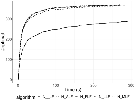
(a) Cumulative number of optima.

Algorithm	Score
N_MLF	1612
N_ALF	1644
N_FLF	1650
N_LLF	1712
N__LF	1932

(b) Borda ranking.

Figure 8: Evaluation of filtering rules.

First, all algorithms find feasible solutions for more than 99% of the instances. Then, for each algorithm, the number of instances solved optimally is drawn as a function of the time in Figure 8(a). The leftmost curve is the fastest whereas the topmost curve proves the more optima. Clearly, compared to N__LF, the filtering rules accelerates the proof and allow the optimal solving of around eighty more instances. One can notice that the advanced filtering rules (N_FLF, N_MLF, N_ALF), also slightly improves the proof compared to the simple update of the flow time lower bound (N_LLF). Here, the advanced filtering rules are indistinguishable.

Table 8(b) ranks the filtering rules according to a scoring procedure based on the Borda count voting system [1]. In this procedure, each benchmark instance is treated like a voter who ranks the algorithms. Each algorithm scores points based on their fractional ranking: the algorithms compare equal receive the same ranking number, which is the mean of what they would have under ordinal rankings. Here, the rank only depends on the answer: the solution status (optimum, satisfiable, and unknown); and then the objective value. So, the lower is the score, the better is the algorithm. Once again, advanced rules are really close, and slightly above the simple lower bound update. They clearly outperform the algorithm without cost-based filtering.

5.3 Comparison to the literature

In this section, the best possible algorithms using the ILP model, CP_O model, and CP_N model are compared. Here, the heuristics are used to initialize the solvers, and thus the algorithms IH_SF, OH_LF, NHALF are studied.

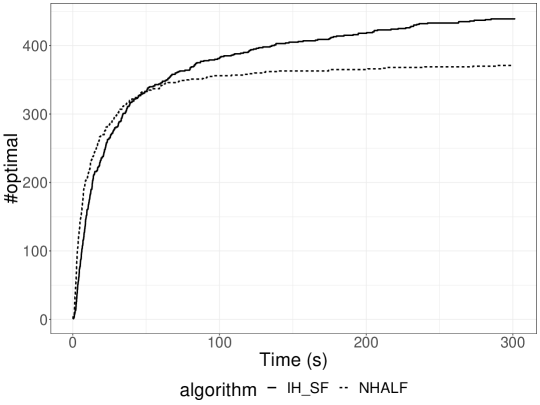
(a) Cumulative number of optima.

Algorithm	Score
IH_SF	942.5
NHALF	951.5
OH_LF	1526.0

(b) Borda ranking.

Figure 9: Comparison of the models.

First, the models exhibit very different behaviors in terms of satisfiability and optimality. Then, for each model, the number of instances solved optimally is drawn as a function of the time in Figure 9(a). The CP_O model is not visible because it does not prove any optimum. The CP_N model is faster than the ILP model, but proves less optima (around seventy).

Table 9(b) ranks the models rules according to the Borda count voting system (see Section 5.2). It confirms the poor efficiency of the CP_O model, but brings closer the performance of CP_N model and ILP model. Table 10(a) explains these close scores. ILP model proves $67=70-3$ more optima than CP_N model, but CP_N model finds feasible solutions for 32 more instances.
To conclude, the CP_N model is competitive with the ILP model and they offer orthogonal performance since the ILP model is more efficient for proving the optimality whereas the CP_N model is more efficient for quickly finding feasible solutions.

5.4 Sensitivity analysis

Here, the impact of the heuristics and of the bi-objective optimization on the efficiency of the models is analyzed. The CP_O model is excluded since it is clearly dominated by the two other models.

The heuristics have a little impact on the CP_N model (see Table 10(a)). The solution status stay identical $98.5\%$ of the time and the solving times remain in the same order of magnitude. However, Table 10(b) shows the significant impact of the heuristics on the ILP model where the answer for 50 instances becomes satisfiable. For both models, the heuristics do not help to prove more optima.
Table 10(c) shows the significant impact of using the lexicographic optimization instead of the weighted sum method on the CP_O model. Indeed, 69 instances with unknown status when using the weighted sum method become satisfiable using the lexicographic optimization. Note that the lexicographic optimization is not available for the ILP model.

NHALF	IH_SF
	OPT	SAT	UNK
OPT	369	3	0
SAT	70	94	32
UNK	1	0	1

(a) Two best algorithms.

I__SF	IH_SF
	OPT	SAT	UNK
OPT	433	3	0
SAT	6	44	0
UNK	1	50	33

(b) Heuristics impact.

N_ALF	N_ASF
	OPT	SAT	UNK
OPT	360	8	1
SAT	4	125	69
UNK	0	0	3

(c) Aggregation impact.

Figure 10: Contingency table of the solution status between pairs of algorithms.

6 Conclusion

In this paper, cost-based domain filtering has been successfully applied to an efficient constraint programming model for scheduling problems with setup on parallel machines. The filtering rules derive from a polynomial-time algorithm which minimize the flow time for a single machine relaxation. Experimental results have shown the rules efficiency and the competitiveness of the overall algorithm. The first perspective is to tackle larger industrial instances since CP relies on its ability at finding feasible solutions. The second perspective is to pay more attention to the propagation of the flow time based on what has been done for the makespan.

References

- Brams and Fishburn [2002] Steven J. Brams and Peter C. Fishburn. Voting procedures. In K. J. Arrow, A. K. Sen, and K. Suzumura, editors, Handbook of Social Choice and Welfare, volume 1 of Handbook of Social Choice and Welfare, chapter 4, pages 173–236. Elsevier, 2002. URL https://ideas.repec.org/h/eee/socchp/1-04.html.
- Ehrgott [2000] M. Ehrgott. Multicriteria optimization. Springer-Verlag, 2000.
- Focacci et al. [1999] F. Focacci, A. Lodi, and M. Milano. Cost-based domain filtering. In Joxan Jaffar, editor, Principles and Practice of Constraint Programming – CP’99, pages 189–203, Berlin, Heidelberg, 1999. Springer Berlin Heidelberg. ISBN 978-3-540-48085-3.
- IBM [2020] IBM. IBM ILOG CPLEX Optimization Studio. https://www.ibm.com/products/ilog-cplex-optimization-studio, 2020.
- Laborie and Rogerie [2008] Philippe Laborie and Jerome Rogerie. Reasoning with conditional time-intervals. In Proceedings of the Twenty-First International Florida Artificial Intelligence Research Society Conference, May 15-17, 2008, Coconut Grove, Florida, USA, pages 555–560, 2008. URL http://www.aaai.org/Library/FLAIRS/2008/flairs08-126.php.
- Laborie et al. [2009] Philippe Laborie, Jerome Rogerie, Paul Shaw, and Petr Vilím. Reasoning with conditional time-intervals. part II: an algebraical model for resources. In Proceedings of the Twenty-Second International Florida Artificial Intelligence Research Society Conference, May 19-21, 2009, Sanibel Island, Florida, USA, 2009. URL http://aaai.org/ocs/index.php/FLAIRS/2009/paper/view/60.
- Malapert and Nattaf [2019] Arnaud Malapert and Margaux Nattaf. A new cp-approach for a parallel machine scheduling problem with time constraints on machine qualifications. In Louis-Martin Rousseau and Kostas Stergiou, editors, Integration of Constraint Programming, Artificial Intelligence, and Operations Research, pages 426–442. Springer International Publishing, 2019. ISBN 978-3-030-19212-9.
- Malapert and Nattaf [2020] Arnaud Malapert and Margaux Nattaf. Minimizing Flow Time on a Single Machine with Job Families and Setup Times. Publication soumise et acceptée à la conférence Project Management and Scheduling (PMS2020)., May 2020. URL https://hal.archives-ouvertes.fr/hal-02530703.
- Mason and Anderson [1991] A. J. Mason and E. J. Anderson. Minimizing flow time on a single machine with job classes and setup times. Naval Research Logistics (NRL), 38(3):333–350, 1991. doi: 10.1002/1520-6750(199106)38:3¡333::AID-NAV3220380305¿3.0.CO;2-0. URL https://onlinelibrary.wiley.com/doi/abs/10.1002/1520-6750%28199106%2938%3A3%3C333%3A%3AAID-NAV3220380305%3E3.0.CO%3B2-0.
- Nattaf et al. [2019] Margaux Nattaf, Stéphane Dauzère-Pérès, Claude Yugma, and Cheng-Hung Wu. Parallel machine scheduling with time constraints on machine qualifications. Comput. Oper. Res., 107:61–76, 2019. doi: 10.1016/j.cor.2019.03.004. URL https://doi.org/10.1016/j.cor.2019.03.004.
- Obeid et al. [2014] Ali Obeid, Stéphane Dauzère-Pérès, and Claude Yugma. Scheduling job families on non-identical parallel machines with time constraints. Annals of Operations Research, 213(1):221–234, Feb 2014. ISSN 1572-9338. doi: 10.1007/s10479-012-1107-4.
- Smith [1956] Wayne E. Smith. Various optimizers for single-stage production. Naval Research Logistics Quarterly, 3(1‐2):59–66, 1956. doi: 10.1002/nav.3800030106. URL https://onlinelibrary.wiley.com/doi/abs/10.1002/nav.3800030106.