A Semi-Parametric Bayesian Generalized Least Squares Estimator

In this paper we propose a semi-parametric Bayesian Generalized Least Squares estimator. In a generic setting where each error is a vector, the parametric Generalized Least Square estimator maintains the assumption that each error vector has the same distributional parameters. In reality, however, errors are likely to be heterogeneous regarding their distributions. To cope with such heterogeneity, a Dirichlet process prior is introduced for the distributional parameters of the errors, leading to the error distribution being a mixture of a variable number of normal distributions. Our method let the number of normal components be data driven. Semi-parametric Bayesian estimators for two specific cases are then presented: the Seemingly Unrelated Regression for equation systems and the Random Effects Model for panel data. We design a series of simulation experiments to explore the performance of our estimators. The results demonstrate that our estimators obtain smaller posterior standard deviations and mean squared errors than the Bayesian estimators using a parametric mixture of normal distributions or a normal distribution. We then apply our semi-parametric Bayesian estimators for equation systems and panel data models to empirical data.

JEL Classification Code: C11, C14, C23, C31

Keywords: Bayesian semi-parametric, generalized least square, Dirichlet process, equation system, Seemingly Unrelated Regression, panel data, Random Effects Model.

1 Introduction

The Generalized Least Square (gls) estimator is a family of econometric methods that have seen numerous applications in empirical economics. As pointed out by Wooldridge (2003), parametric gls type estimators accommodate a deviation from the assumption that the errors in the model are homoskedastic and have no serial correlation. For example, compared to the ordinary least squares regression model, gls no longer assumes that the covariance matrix of the errors is diagonal with identical diagonal elements.

In a more general setting, each error may be a random vector, which includes some of the most popular applications of gls. For example, the Seemingly Unrelated Regression (sur, Zellner, 1962 and 1971) has been developed for equation systems, and widely applied to gain efficiency by exploiting the correlation between errors across equations. Similarly, in the analysis of panel data the random effects model (rem) recognizes that there are individual specific, time-invariant features that are unobservable and uncorrelated with the explanatory variables.

However, the parametric gls still maintains the assumption that the error vector of each individual has the same covariance matrix. In reality, however, heterogeneity in error distributions is a major concern in empirical analyses. Such heterogeneity can be caused by observations on individuals or households reflecting variation in features such as the size of the household and the level of income, among others. It is a challenge for analysts who seek efficient estimates and inference with the data to capture the form of the heterogeneity in observations.

The standard Bayesian approach to gls assumes that the error distribution is multivariate normal. Recent developments in Bayesian methods allow the use of prior information to relax this assumption. The Dirichlet prior has been introduced to accommodate heterogeneity in the distributions of both errors (see Chigira and Shiba, 2015 for an example) and model parameters (Allenby et al., 1998) by mixing a fixed number of normal distributions.

A notable drawback of the Dirichlet prior is that the the dimension of the mixing distribution is usually unknown. Bayesian semi-parametric methods introduce more flexibility by letting the data and the prior determine the structure of heterogeneity jointly. The Dirichlet Process ($\mathcal{DP}$) prior can be used to form a mixing of normal distributions, whose dimension need not be predetermined. In this sense, the use of $\mathcal{DP}$ priors represents a more flexible approach to accommodating heterogeneity than the mixing of a fixed number of normal distributions with the Dirichlet prior.

In the context where heterogeneity in the distributions of errors is a major concern, $\mathcal{DP}$ priors are introduced for the distributional parameters of the errors in the model. Under this prior, the distributional parameters are put into groups, and assigned a group specific value. As a result, the corresponding errors will have group specific distributions.

A landmark study in this area is Conley et al. (2008), who introduce a Bayesian semi-parametric approach to the instrumental variable problem in a two stage least square type model. Due to the endogeneity of some explanatory variables, the errors in the two stages are correlated by construction. Instead of assuming that the joint errors in the two stages have an identical bivariate normal distribution (c.f., Chao and Phillips, 1998; Geweke, 1996; Kleibergen and van Dijk, 1998; Rossi et al., 2005), the authors introduce a Dirichlet process prior for the distributional parameters. This provides a semi-parametric version of two stage least squares, where the errors of the two stages jointly follow a non-parametric mixture of normal distributions.

In this paper we focus on relaxing the identical distribution assumption on the errors, but in a different scenario from that of Conley et al. (2008). We propose a semi-parametric Bayesian gls that incorporates the $\mathcal{DP}$ prior. The motivation is to incorporate more information in the error distribution by allowing their distributional parameters to differ across observations. The resulting distribution of the error terms will involve a mixture of normal distributions where the number of the normal components is influenced by both the prior and the data. We then introduce two specific cases of semi-parametric Bayesian gls, namely for equation systems and panel data.

The rest of the paper is organized as follow. In Section 2 we briefly review the literature on the Dirichlet process and its application as a prior for semi-parametric Bayesian estimators. We then consider two special cases of the gls. The sur with the $\mathcal{DP}$ prior (dp-sur) is introduced in Section 3 with simulation and empirical results. Section 4 motivates and introduces our semi-parametric Bayesian gls estimator for the random effects model with the $\mathcal{DP}$ prior (dp-rem) for panel data, together with simulation and empirical results. Section 5 concludes the paper.

2 Bayesian GLS with Dirichlet Process Prior

In this section we introduce the generic form of Bayesian gls with the $\mathcal{DP}$ prior. In Section 2.1 we briefly review the literature in related areas. In Section 2.2 we introduce the semi-parametric Bayesian gls.

2.1 Literature Review

Bayesian attempts to incorporate heterogeneity in the distributional parameters of the errors in the linear regression model can be traced back to Geweke (1993) with the use of an inverse gamma prior for the variances of the errors. He demonstrates that such a scale mixture of normal distributions is equivalent to the errors having a t-distribution.

Although the model with the t-distributed errors is more flexible than assuming a normal distribution for the errors, this approach depends upon the assumption that the normal distributions are mixed with inverse gamma distributed variances. As pointed out by Koop (2003), relaxing this assumption results in more flexible models, given that the errors are no longer restricted to having a t-distribution. This can be done by using a Dirichlet prior, the conjugate prior of a multinomial distribution, to mix a finite number of normal distributions.

The Dirichlet mixture model has emerged as a widely applied methodology for capturing heterogeneity in both linear and non-linear models, c.f., Allenby et al. (1998), Li and Tobias (2011) and Chigira and Shiba (2015). The main limitation is that it takes a fairly difficult test procedure to determine the “correct” number of mixing components.

In the wake of this limitation of the Dirichlet mixture model, it seems more reasonable to let the data and the prior jointly determine the number of normal components in the mixture. This can be achieved using a Dirichlet prior of infinite dimension, which is the Dirichlet process ($\mathcal{DP}$) introduced by Ferguson (1973). $\mathcal{DP}$ is the conjugate prior for a non-parametric multinomial distribution of infinite dimensions. The generic form of the $\mathcal{DP}$ can be written as

$$F\sim\mathcal{DP}\left(\alpha,F_{0}\right),$$ (1)

where $\alpha>0$ is the concentration parameter, and $F_{0}$ is the base distribution. $F$ is a random distribution that is discrete with probability one.

The $\mathcal{DP}$ is a non-parametric “distribution of distributions” (Escobar and West, 1995 and 1998; MacEachern, 1998), in the sense that a draw, say $F$, from a $\mathcal{DP}$ is a probability distribution itself. Conditional on $n-1$ existing realizations $\{r_{1},r_{2},\ldots,r_{n-1}\}$ from $F$, the Chinese restaurant process (Aldous, 1985) provides the predictive probabilities of the $n^{th}$ realization, $r_{n}$. Due to the fact that $F$ is discrete, the existing realizations will be assigned to groups, where all realizations in the same group take a group specific unique value.

Denote the group id of $r_{i}$ as $c_{i}=1,\ldots,K$, and the unique value of group $c_{i}$ as $r_{c_{i}}^{*}$: if $r_{i}$ is in group $k$, then $r_{i}=r_{c_{i}}^{*}=r_{k}^{*}$. The prediction probabilities of $r_{n}$ is given by

$$\Pr\left\{r_{n}=r^{*}_{k}|r_{1},r_{2},\ldots,r_{n-1}\right\}=\left\{\begin{array}[]{ll}\frac{n_{k}}{n-1+\alpha}&\text{if}\ 1\leq k\leq K\\ &\\ \frac{\alpha}{n-1+\alpha}&\text{if}\ k=K+1\ (\text{i.e.,}\ r_{n}=r^{*}_{K+1}\sim F_{0})\end{array}\right.,$$ (2)

where $n_{k}$ is the number of realizations that are already in group $k$. Aldous (1985) show that $r_{1},r_{2},\ldots,r_{n}$ generated according to the Chinese restaurant process are i.i.d. draws from $F$, i.e.,

$$F|\alpha,F_{0} \sim\mathcal{DP}(\alpha,F_{0})$$ (3)

$$r_{i}|F \overset{iid}{\sim}F.$$

A model with a $\mathcal{DP}$ prior on the distribution of parameters is called a $\mathcal{DP}$ mixture model (c.f., de Carvalho et al., 2013; Wiesenfarth et al., 2014; Li et al., 2018 and Hejblum et al., 2019), and is capable of representing very general forms of heterogeneity in the distributions of the observations. The $\mathcal{DP}$ normal mixture model, whose mixture components are normal distributions, can be written as

$$F|\alpha,F_{0} \sim\mathcal{DP}(\alpha,F_{0})$$ (4)

$$\theta_{i}|F \overset{iid}{\sim}F$$

$$\bm{y}_{i}|\theta_{i} \sim\mathcal{N}\left(\theta_{i}\right),$$

where $\theta_{i}$ is the set of parameters of observation $\bm{y}_{i}$. In the multivariate normal case, $\theta_{i}$ consists of the mean vector and covariance matrix, i.e., $\theta_{i}=\left(\bm{\mu}_{i},\bm{\Sigma}_{i}\right)$.

The posterior probability of $\theta_{i}$ having the same value as one of the existing $\theta_{-i}$ is

$$\Pr\left\{\theta_{i}=\theta^{*}_{k}|\theta_{-i},\bm{y}_{i},\alpha\right\}\propto\frac{n_{k}}{n-1+\alpha}f_{\mathcal{N}}\left(\bm{y}_{i}|\theta^{*}_{k}\right),$$ (5)

where $\theta^{*}_{k}$ and $n_{k}$ respectively denote the unique value of group $k$ and the number of observations already in group $k$. $f_{\mathcal{N}}(\cdot)$ denotes the density function of multivariate normal distribution. The posterior probability of $\theta_{i}$ taking a new value $\theta^{*}_{new}$ from the base distribution is

$$\Pr\left\{\theta_{i}=\theta^{*}_{new}|\theta_{i},\bm{y}_{i},\alpha,F_{0}\right\}\propto\frac{\alpha}{n-1+\alpha}\int f_{\mathcal{N}}\left(\bm{y}_{i}|\theta_{i}\right)f_{F_{0}}\left(\theta_{i}\right)\mathop{}\!\mathrm{d}\theta_{i},$$ (6)

where $f_{F_{0}}\left(\theta_{i}\right)$ is the probability density of the current value $\theta_{i}$ given $F_{0}$.

2.2 Semi-parametric Bayesian GLS

In this section we introduce the generic form of the semi-parametric gls estimator, where a $\mathcal{DP}$ prior is introduced on the distributional parameters of the errors. Consider a general linear regression

$$\bm{y}_{i}=\bm{X}_{i}\bm{\beta}+\bm{\varepsilon}_{i},$$ (7)

where $i$ indexes the observation, $\bm{y}_{i}$ is a $Q\times 1$ vector of dependent variables, $\bm{X_{i}}$ is a $Q\times K$ matrix of explanatory variables, and $\bm{\beta}$ is a $K\times 1$ vector of coefficients. $\bm{\varepsilon}_{i}\sim\mathcal{N}\left(\theta_{i}\right)$ is a $Q\times 1$ vector of errors, where $\theta_{i}=\left(\bm{\mu}_{i},\bm{\Sigma}_{i}\right)$ denotes the distribution parameters.

To facilitate a more flexible distribution for the errors, where both the mean and covariance matrix of each $\bm{\varepsilon_{i}}$ is allowed to be different, we do not include a constant in $\bm{X}_{i}$. Our semi-parametric gls estimator introduces a $\mathcal{DP}$ prior on the distribution of $\theta_{i}$, resulting in the errors having a non-parametric mixture of normal distributions. The hierarchical prior for $\theta_{i}$ is

$$F|\alpha,F_{0} \sim\mathcal{DP}(\alpha,F_{0})$$ (8)

$$\theta_{i}|F \overset{iid}{\sim}F,$$

where $\alpha$ is the concentration parameter, and $F_{0}$ is the base distribution of the $\mathcal{DP}$, respectively.

Due to the discreteness of $F$ under the $\mathcal{DP}$ prior, the values of some $\theta_{i}$’s will be the same, thus putting them into the same group. The distribution parameters of $\bm{\varepsilon}_{i}$ can then be written as

$$\theta_{i}=\theta_{c_{i}}^{*}=\left(\bm{\mu}_{c_{i}}^{*},\bm{\Sigma}_{c_{i}}^{*}\right)$$ (9)

where $c_{i}$ denotes the group id of $\bm{\varepsilon}_{i}$, and the superscript $*$ denotes the group-specific values of parameters. If $c_{i}=c_{j}$, $i,j\in\{1,2,\ldots,N\}$, $\bm{\varepsilon}_{i}$ and $\bm{\varepsilon}_{j}$ share the same group id and parameters, i.e., $\bm{\mu}_{c_{i}}^{*}=\bm{\mu}_{c_{j}}^{*}$ and $\bm{\Sigma}_{c_{i}}^{*}=\bm{\Sigma}_{c_{j}}^{*}$. Such “grouping” characteristic can help to reveal the structure of the unobserved heterogeneity in the data.

A straightforward choice of the base distribution is the normal-inverse Wishart distribution, i.e., $\theta\sim\mathcal{NIW}(\nu_{0},\bm{W}_{0},\bm{\lambda}_{0},\kappa_{0})$, or equivalently,

$$\bm{\Sigma} \sim\mathcal{IW}(\nu_{0},\bm{W}_{0}),$$ (10)

$$\bm{\mu}|\bm{\Sigma} \sim\mathcal{N}\left(\bm{\lambda}_{0},\kappa_{0}^{-1}\bm{\Sigma}\right),$$

where $\nu_{0}$, $\bm{W}_{0}$, $\bm{\lambda}_{0}$ and $\kappa_{0}$ are the hyper-parameters of the normal-inverse Wishart distribution. As the normal-inverse Wishart distribution is the conjugate prior for the parameters of a multivariate normal distribution, such a base distribution simplifies the evaluation of the posterior probability of $\theta_{i}$ taking a new value in (6). Having specified the $\mathcal{DP}$ prior, we now outline the process of drawing from the posterior distributions of the parameters.

2.3 MCMC Algorithm

In order to take draws for the parameters in the model, the following Gibbs sampler is employed. We need to draw the distributional parameters $\Theta=\{\theta_{c_{i}}^{*}\}_{i=1}^{N}=\{\bm{\mu}_{c_{i}}^{*},\bm{\Sigma}_{c_{i}}^{*}\}_{i=1}^{N}$, the regression parameters $\bm{\beta}$ and the concentration parameter $\alpha$ of the $\mathcal{DP}$ prior, i.e.,

$$\Theta |\bm{y},\bm{X},\bm{\beta},\alpha$$ (11)

$$\bm{\beta} |\bm{y},\bm{X},\Theta,\alpha$$

$$\alpha |\bm{y},\bm{X},\bm{\beta},\Theta.$$

We begin with drawing the distributional parameters of the errors. For this we view the residuals $\bm{e}_{i}$ ($i=1,\ldots,N$) as the “observed” errors. According to (5) in the Chinese restaurant process, the probability of distributional parameters $\theta_{i}$ being assigned to group $c_{j}$ is

$$\tilde{p}_{j}=\frac{1}{N-1+\alpha}f_{\mathcal{N}}\left(\bm{e}_{i}|\theta^{*}_{c_{j}}\right),\quad\ j\neq i.$$ (12)

Similarly by (6), the probability of $\theta_{i}$ being assigned to a new group, i.e., taking a new value drawn from $F_{0}$ is

$$\tilde{p}_{i}=\frac{\alpha}{N-1+\alpha}\int f_{\mathcal{N}}\left(\bm{e}_{i}|\theta_{i}\right)f_{F_{0}}\left(\theta_{i}\right)\mathop{}\!\mathrm{d}\theta_{i}.$$ (13)

Normalizing $\tilde{p}=\{\tilde{p}_{1},\ldots,\tilde{p}_{N}\}$ gives us a multinomial probability vector

$$p=\frac{\tilde{p}}{\sum_{k=1}^{N}{\tilde{p}_{k}}},\quad\tilde{p}=\left[\tilde{p}_{1},\ldots,\tilde{p}_{N}\right]^{\prime}.$$ (14)

A draw can then be taken within $1,\ldots,N$ from the corresponding multinomial distribution to update the group membership. If the multinomial draw is $j\neq i$, $\theta_{i}$ is assigned to the group $c_{j}$, while if the draw is $i$, $\theta_{i}$ is assigned to a new group.

It should be mentioned that due to the choice of normal-inverse Wishart distribution for $F_{0}$, the integral in (13) is

$$\int f_{\mathcal{N}}\left(\bm{e}_{i}|\theta_{i}\right)p\left(\theta_{i}|F_{0}\right)\mathop{}\!\mathrm{d}\theta_{i}=\frac{1}{\pi^{Q/2}}\frac{\kappa_{0}^{Q/2}\Gamma_{Q}\left(\frac{\nu_{0}+1}{2}\right)|\bm{W_{0}}|^{\nu_{0}/2}}{\left(\kappa_{0}+1\right)^{Q/2}\Gamma_{Q}\left(\frac{\nu_{0}}{2}\right)|\bm{W_{0}}+\bm{S}|^{\left(\nu_{0}+1\right)/2}},$$ (15)

where $Q$ is the dimension of the error term vector $\bm{\varepsilon}_{i}$, $\Gamma_{Q}(\cdot)$ is the multivariate gamma function, and

$$\bm{S}=\frac{\kappa_{0}}{\kappa_{0}+1}\left(\bm{e}_{i}-\bm{\lambda}_{0}\right)\left(\bm{e}_{i}-\bm{\lambda}_{0}\right)^{\prime}.$$ (16)

As for the value of the hyper-parameters, we follow Conley et al. (2008) and set $\nu_{0}=Q+0.004$, $\bm{W}_{0}=0.17\bm{I}$, $\bm{\lambda}_{0}=\bm{0}$ and $\kappa_{0}=0.016$.

Once the group memberships of all the distributional parameters $\theta_{i}$ have been updated, the unique values of parameters for each group are redrawn (as suggested by Escobar and West, 1998). Let $N_{k}$ and $\bar{\bm{e}}_{k}$ be the number of residuals assigned to group $k$ and their sample mean, respectively. The unique values of this group $\theta_{k}^{*}=(\bm{\mu}_{k}^{*},\bm{\Sigma}_{k}^{*})$ is redrawn from a normal-inverse Wishart distribution denoted by $\mathcal{NIW}(\nu_{k},\bm{W}_{k},\bm{\lambda}_{k},\kappa_{k})$, whose parameters are

$$\nu_{k} =\nu_{0}+N_{k}$$ (17)

$$\kappa_{k} =\kappa_{0}+N_{k}$$

$$\bm{\lambda}_{k} =\kappa_{k}^{-1}\left(\kappa_{0}\bm{\lambda}_{0}+N_{k}\bar{\bm{e}}\right)$$

$$\bm{W}_{k} =\bm{W}_{0}+\bm{S}_{k}+\frac{\kappa_{0}N_{k}}{\kappa_{0}+N_{k}}\left(\bar{\bm{e}}_{k}-\bm{\lambda}_{0}\right)\left(\bar{\bm{e}}_{k}-\bm{\lambda}_{0}\right)^{\prime},$$

where $\bm{S}_{k}=\sum_{c_{i}=k}{\left(\bm{e}_{i}-\bar{\bm{e}}_{k}\right)\left(\bm{e}_{i}-\bar{\bm{e}}_{k}\right)^{\prime}}$.

After draws have been taken for the distributional parameters, we move on to the second part of the mcmc algorithm in (11), which draws from the posterior of the regression parameters $\bm{\beta}$. The likelihood of $\bm{\beta}$ in (7) is

$$p\left(\bm{y}_{i}|\bm{\beta},\bm{\mu}_{c_{i}}^{*},\bm{\Sigma}_{c_{i}}^{*}\right)=\frac{1}{(2\pi)^{Q/2}}|\bm{\Sigma}_{c_{i}}^{*}|^{-\frac{1}{2}}\exp\left[-\frac{1}{2}(\bm{y}_{i}-\bm{X}_{i}\bm{\beta}-\bm{\mu}_{c_{i}}^{*})^{\prime}\bm{\Sigma}_{c_{i}}^{*-1}(\bm{y}_{i}-\bm{X}_{i}\bm{\beta}-\bm{\mu}_{c_{i}}^{*})\right].$$ (18)

We specify a normal prior for $\bm{\beta}$, i.e.,

$$\bm{\beta}\sim\mathcal{N}(\bm{b}_{0},\bm{V}_{0}),$$ (19)

where $\bm{b}_{0}$ and $\bm{V}_{0}$ denote the prior mean and covariance matrix of $\bm{\beta}$, respectively. The posterior of $\bm{\beta}$ is

$$\bm{\beta}|\bm{y},\bm{\mu}_{c_{i}}^{*},\bm{\Sigma}_{c_{i}}^{*}\sim\mathcal{N}(\bm{b},\bm{V}),$$ (20)

where

$$\bm{V}=\left(\bm{V}_{0}^{-1}+\sum_{i=1}^{N}{\bm{X}_{i}^{\prime}\bm{\Sigma}_{c_{i}}^{*-1}\bm{X}_{i}}\right)^{-1},$$ (21)

and

$$\bm{b}=\bm{V}\left(\bm{V}_{0}^{-1}\bm{b}_{0}+\sum_{i=1}^{N}{\bm{X}_{i}^{\prime}\bm{\Sigma}_{c_{i}}^{*-1}(\bm{y}_{i}-\bm{\mu}_{c_{i}}^{*})}\right).$$ (22)

For the hyper-parameters we specify $\bm{b}_{0}=\bm{0}$ and $\bm{V}_{0}=1000\bm{I}_{K}$, in order to prevent a prior that is overly informative.

Finally, to make draws of the concentration parameter $\alpha$, we adopt the prior introduced by Conley et al. (2008), which is

$$p(\alpha)\propto\left(1-\frac{\alpha-\alpha_{min}}{\alpha_{max}-\alpha_{min}}\right)^{\tau},$$ (23)

where $\alpha_{min}$ and $\alpha_{max}$ are the pre-set lower and upper bounds of $\alpha$. Larger $\alpha$ leads to more groups being generated on average, i.e., the $\mathcal{DP}$ being less discrete. Antoniak (1974) gives the distribution of $K$, the number of groups, conditioned on $\alpha$. The corresponding posterior of $\alpha$ is

$$p(\alpha|K)\propto\alpha^{K}\frac{\Gamma(\alpha)}{\Gamma(N+\alpha)}\left(1-\frac{\alpha-\alpha_{min}}{\alpha_{max}-\alpha_{min}}\right)^{\tau},\ \alpha\in\left(\alpha_{min},\alpha_{max}\right).$$ (24)

We set $\alpha_{min}$ to 0.1083 such that the mode of $K$ is 1, and set $\alpha_{max}$ to 1.834 so that the mode of $K$ is 5% of the sample size. Following the suggestion of Conley et al. (2008), we set $\tau$ to 0.8.

3 Semi-parametric Seemingly Unrelated Regression

In this section we introduce how the $\mathcal{DP}$ prior is incorporated with the sur for equation systems. Consider a system of $M$ equations

$$\bm{y}_{m}=\bm{X}_{m}\bm{\beta}_{m}+\bm{\varepsilon}_{m},\quad m=1,\ldots,M,$$ (25)

where $\bm{y}_{m}=\left[y_{mi}\right]_{m=1}^{M}$, $\bm{\varepsilon}_{m}=\left[\varepsilon_{mi}\right]_{m=1}^{M}$ are $N\times 1$ vectors of dependent variables and errors, respectively. $\bm{X}_{m}$ is an $N\times K_{m}$ matrix of explanatory variables. Following our assumptions in 2.2, there are no constants in the equations. $\bm{\beta}_{m}$ is a $K_{m}\times 1$ vector of parameters.

3.1 DP Prior for SUR

In the presence of correlation between errors across the equations there exists an efficiency gain by utilising a system estimator. The sur (Zellner, 1962) was introduced for this task. The equations are stacked in the following way

$$\begin{bmatrix}\bm{y}_{1}\\ \vdots\\ \bm{y}_{M}\\ \end{bmatrix}=\begin{bmatrix}\bm{X}_{1}&\cdots&\bm{0}\\ \vdots&\ddots&\vdots\\ \bm{0}&\cdots&\bm{X}_{M}\\ \end{bmatrix}\begin{bmatrix}\bm{\beta}_{1}\\ \vdots\\ \bm{\beta}_{M}\\ \end{bmatrix}+\begin{bmatrix}\bm{\varepsilon}_{1}\\ \vdots\\ \bm{\varepsilon}_{M}\\ \end{bmatrix},$$ (26)

or simply

$$\bm{y}=\bm{X\beta}+\bm{\varepsilon}.$$ (27)

In comparison with the Bayesian ols estimator that usually assumes $\varepsilon_{mi}\overset{iid}{\sim}\mathcal{N}(\mu_{m},\sigma_{m}^{2})$ for all $m$, the errors $\bm{\varepsilon}_{i}$ are now identically multivariate normally distributed, i.e., $\bm{\varepsilon}_{i}\overset{iid}{\sim}\mathcal{N}(\bm{\mu},\bm{\Sigma})$. The covariance matrix of $\bm{\varepsilon}$ is then

$$\bm{\Omega}=\bm{\Sigma}\otimes\bm{I}=\begin{bmatrix}\sigma_{11}\bm{I_{N}}&\cdots&\sigma_{1M}\bm{I_{N}}\\ \vdots&\ddots&\vdots\\ \sigma_{M1}\bm{I_{N}}&\cdots&\sigma_{MM}\bm{I_{N}}\\ \end{bmatrix},\ \text{s.t.}\ \sigma_{pq}=\sigma_{qp},\ p,q=1,\ldots,M,$$ (28)

where ”$\otimes$” stands for the Kronecker product.

The gls type estimators (sur in this case) utilize the information in the covariance matrix to transform the data, so that the transformed errors are homoskedastic with no serial correlation. Such transformation is reflected in the likelihood as in (18). The prior and posterior of the parameters can be defined similarly to equations (19) to (22).

Although sur accounts for the cross-equation correlation of errors, as Wooldridge (2003) has noted, the errors are assumed to be identically distributed. Moreover, unlike the frequentist gls estimator, this distribution is usually assumed to be normal in Bayesian methods. In this section we propose a new dp-sur estimator that makes no a priori assumptions on the family of distribution of the errors. If we allow each observation $i$ to have its own distributional parameters, flexibility of the error distribution will lead to identification problems given cross sectional data. A compromise is to assign the observations into groups with the $\mathcal{DP}$ prior as in (8), in which case the distribution parameters of $\bm{\varepsilon}_{i}$ of the sur in (26) is

$$\bm{\mu}_{c_{i}}^{*}=\begin{bmatrix}\mu_{1,c_{i}}^{*}\\ \vdots\\ \mu_{M,c_{i}}^{*}\\ \end{bmatrix};\quad\bm{\Sigma}_{c_{i}}^{*}=\begin{bmatrix}\sigma_{11,c_{i}}^{*}&\cdots&\sigma_{1M,c_{i}}^{*}\\ \vdots&\ddots&\vdots\\ \sigma_{M1,c_{i}}^{*}&\cdots&\sigma_{MM,c_{i}}^{*}\\ \end{bmatrix},\ s.t.\ \sigma_{pq,c_{i}}^{*}=\sigma_{qp,c_{i}}^{*},\ p,q=1,\ldots,M.$$ (29)

The main difference from the parametric Bayesian sur is that the covariance matrix of each observation is now given in (29), which allows each group of observations to have its own unique values for the parameters. Then draws can be taken from the posteriors of parameters according to the Gibbs sampler described in Section 2.3.

3.2 A Simulation Experiment

In this section we conduct simulation experiments designed to evaluate and compare the performances of three estimators. The first one is our semi-parametric dp-sur in Section 3.1. The second is a Bayesian sur, where the errors have a parametric mixture of normal distributions with a Dirichlet prior (abbreviated as dir-sur hereafter) on the distributional parameters of the errors. The third is a parametric Bayesian sur where the errors have a normal distribution (abbreviated as nor-sur hereafter).

With not loss of generality, all simulation experiments are based on a two-equation system. Two explanatory variables are included in each equation, which are drawn from normal distributions with the following parameters

$$x_{11,i}\overset{iid}{\sim}\mathcal{N}(5,2),\ x_{12,i}\overset{iid}{\sim}\mathcal{N}(6,2),$$

and

$$x_{21,i}\overset{iid}{\sim}\mathcal{N}(-5,2),\ x_{22,i}\overset{iid}{\sim}\mathcal{N}(6,2).$$

We set the values of the parameters to $\bm{\beta}_{1}=(1,-2)^{\prime}$ and $\bm{\beta}_{2}=(-1,2)^{\prime}$.

We generate errors from two types of distributions to demonstrate our dp-sur. The first is the multivariate log-normal distribution, i.e., $\ln\bm{\varepsilon_{i}}\sim\mathcal{N}\left(\bm{0},\bm{\Sigma}\right)$. The log-normal distribution is fat tailed with a positive mean, thus suitable for examining the performance of our semi-parametric dp-sur. For the covariance matrix of the bivariate normal distribution of $\ln\bm{\varepsilon}_{i}$, we specify its form as

$$\bm{\Sigma}=\begin{bmatrix}\sigma^{2}&0.5\sigma^{2}\\ 0.5\sigma^{2}&\sigma^{2}\\ \end{bmatrix}.$$

Without loss of generality, we let the variances of $\varepsilon_{1i}$ and $\varepsilon_{2i}$ be identical, and fix the correlation between them at 0.5. In order to explore the performances of the estimators when extreme values are generated with different probabilities, we set $\sigma^{2}$ equal to three values: 1, 1.5 and 2.

The second type of error distribution is designed to demonstrate the performance of our dp-sur when the errors have multi-modal distributions. In order to adjust the heaviness of the tails of the distributions as well, we employ mixtures of multivariate Student t distributions, which are scale mixtures of multivariate normal distributions (Andrews and Mallows, 1974). To avoid unnecessary complexity, we utilise a mixture of two multivariate t distributions with the same degrees of freedom ($df$) and scale matrix, but with different means. More specifically, the scale matrix shared by both multivariate t distributions is

$$\bm{\Sigma}=\begin{bmatrix}1&0.5\\ 0.5&1\\ \end{bmatrix}.$$

Four $df$ are specified to adjust the heaviness of the tails of the mixture distribution, namely 2, 4, 6 and $\infty$, with the tails becoming less heavy. Note that when the $df$ is $\infty$, the mixture distribution reduces to a mixture of multivariate normal distributions. The mean vectors of the two multivariate t are $[-1,-1]^{\prime}$ and $[4,4]^{\prime}$. They are chosen to ensure that the mean vectors of the two mixture components are located far enough from one another, so that the mixture distributions are bi-modal for all four $df$. The two multivariate t distributions are allocated mixture weights of 0.4 and 0.6, respectively, resulting in the mixture distributions being asymmetric.

Three sample sizes are chosen for the simulation experiments: 100, 200, and 300. For each sample size, 100 samples are generated. In the following section we will report the average posterior means, standard deviations and mean squared errors over the 100 samples.

3.3 DP-SUR Simulation Results

In this section we present the results of the simulations for the three estimators dp-sur, dir-sur and nor-sur.

3.3.1 Results with Log-normal Distributions

In Table 1 we report the posterior means, standard deviations and the mean squared errors of the parameters averaged over the 100 samples, estimated with the three estimators when the errors are multivariate log-normal. The columns are divided into three blocks for the three sample sizes, each containing the results of the three estimators. The rows are also divided into three blocks for the three values of the variance $\sigma^{2}$. Each block contains the posterior mean, standard deviation and mean squared errors of the parameters. It should be noted that the dir-sur uses a fixed number of mixture components, which in our simulation studies is set to the posterior mode of the number of clusters given by the dp-sur averaged over the 100 samples.

Table 1: Simulation Results for SUR with Log-normal Distributions

	$N$	100				200				300
	Estimator	DP	DIR	NOR		DP	DIR	NOR		DP	DIR	NOR
	Parameter						$\sigma^{2}=1$
Mean	$\beta_{11}$	1.0036	1.0084	1.0050		1.0027	1.0032	1.0078		1.0004	1.0000	0.9972 [t]
	$\beta_{12}$	-1.9934	-1.9947	-1.9964		-1.9943	-1.9963	-1.9927		-1.9987	-1.9978	-1.9957
	$\beta_{21}$	-1.0039	-1.0002	-0.9972		-1.0037	-1.0089	-1.0152		-1.0022	-1.0085	-1.0127
	$\beta_{22}$	2.0026	2.0056	2.0060		1.9999	1.9991	1.9962		2.0026	1.9995	1.9977 [b]
SD	$\beta_{11}$	0.0254	0.0653	0.0865		0.0186	0.0603	0.0783		0.0128	0.0443	0.0561 [t]
	$\beta_{12}$	0.0273	0.0676	0.0927		0.0173	0.0543	0.0707		0.0125	0.0423	0.0549
	$\beta_{21}$	0.0274	0.0754	0.1022		0.0162	0.0535	0.0692		0.0144	0.0484	0.0615
	$\beta_{22}$	0.0273	0.0733	0.1012		0.0179	0.0572	0.0771		0.0131	0.0435	0.0564 [b]
MSE	$\beta_{11}$	0.0014	0.0080	0.0263		0.0007	0.0060	0.0145		0.0004	0.0037	0.0079 [t]
	$\beta_{12}$	0.0016	0.0095	0.0220		0.0008	0.0053	0.0099		0.0003	0.0030	0.0067
	$\beta_{21}$	0.0013	0.0097	0.0227		0.0005	0.0046	0.0099		0.0004	0.0044	0.0093
	$\beta_{22}$	0.0017	0.0086	0.0219		0.0007	0.0048	0.0120		0.0003	0.0031	0.0062 [b]
							$\sigma^{2}=1.5$
Mean	$\beta_{11}$	1.0020	1.0045	0.9845		1.0008	0.9972	0.9943		1.0004	1.0012	1.0026 [t]
	$\beta_{12}$	-1.9952	-1.9884	-1.9806		-1.9967	-2.0005	-2.0042		-1.9994	-1.9968	-2.0067
	$\beta_{21}$	-1.0034	-0.9948	-0.9912		-0.9988	-1.0030	-0.9893		-0.9991	-0.9974	-0.9901
	$\beta_{22}$	2.0016	2.0002	1.9912		1.9970	1.9983	1.9954		1.9991	2.0069	2.0191 [b]
SD	$\beta_{11}$	0.0276	0.0986	0.1661		0.0154	0.0709	0.1172		0.0126	0.0647	0.1026 [t]
	$\beta_{12}$	0.0292	0.0999	0.1758		0.0169	0.0731	0.1283		0.0123	0.0614	0.1015
	$\beta_{21}$	0.0280	0.1051	0.1683		0.0159	0.0711	0.1177		0.0117	0.0598	0.0913
	$\beta_{22}$	0.0252	0.0949	0.1543		0.0172	0.0727	0.1227		0.0116	0.0574	0.0904 [b]
MSE	$\beta_{11}$	0.0017	0.0144	0.0676		0.0005	0.0078	0.0296		0.0003	0.0058	0.0234 [t]
	$\beta_{12}$	0.0018	0.0170	0.0825		0.0006	0.0082	0.0377		0.0003	0.0058	0.0197
	$\beta_{21}$	0.0017	0.0172	0.0613		0.0005	0.0082	0.0354		0.0003	0.0059	0.0188
	$\beta_{22}$	0.0014	0.0145	0.0618		0.0006	0.0084	0.0391		0.0003	0.0051	0.0214 [b]
							$\sigma^{2}=2$
Mean	$\beta_{11}$	1.0021	1.0039	0.9854		1.0031	1.0051	1.0084		1.0010	1.0098	1.0142 [t]
	$\beta_{12}$	-1.9950	-1.9876	-1.9762		-2.0010	-1.9938	-2.0108		-1.9980	-2.0010	-2.0179
	$\beta_{21}$	-1.0041	-1.0165	-1.0213		-0.9991	-0.9995	-0.9855		-1.0001	-1.0075	-1.0154
	$\beta_{22}$	2.0082	2.0205	2.0655		2.0028	2.0117	1.9899		2.0003	1.9995	1.9927 [b]
SD	$\beta_{11}$	0.0263	0.1197	0.2767		0.0166	0.0989	0.2247		0.0117	0.0777	0.1600 [t]
	$\beta_{12}$	0.0294	0.1249	0.3173		0.0172	0.0975	0.2358		0.0121	0.0755	0.1637
	$\beta_{21}$	0.0263	0.1265	0.2716		0.0168	0.0983	0.2135		0.0111	0.0767	0.1598
	$\beta_{22}$	0.0278	0.1276	0.2941		0.0151	0.0881	0.1959		0.0112	0.0749	0.1647 [b]
MSE	$\beta_{11}$	0.0017	0.0207	0.3210		0.0006	0.0131	0.1264		0.0003	0.0092	0.0609 [t]
	$\beta_{12}$	0.0021	0.0239	0.2620		0.0007	0.0135	0.1239		0.0003	0.0083	0.0683
	$\beta_{21}$	0.0014	0.0224	0.1950		0.0006	0.0136	0.1332		0.0003	0.0081	0.0690
	$\beta_{22}$	0.0017	0.0262	0.2690		0.0005	0.0117	0.0933		0.0002	0.0088	0.0834 [b]

One may see from Table 1 that all three estimators give posterior means that are very close to the true values of the parameters. This indicates that all three estimators provide good point estimators for the parameters.

Regarding the posterior standard deviations, it is not surprising that all three estimators provide smaller posterior deviations when the sample size increases for each of the three $\sigma^{2}$. Table 1 also shows that the dp-sur posterior standard deviations are uniformly smaller than the dir-sur ones, which are in turn smaller than the nor-sur posterior standard deviations. It is worth noticing that when $\sigma^{2}$ gets larger, the ratio of the dp-sur posterior standard deviations to the dir-sur become smaller for all sample sizes. This indicates that through a non-parametric mixture of normal distributions, our dp-sur achieves increasingly less dispersed posteriors than the dir-sur that employs a parametric mixture when the “true” distribution of the errors is more skewed and heavy tailed.

The same phenomena are also observed comparing the dp-sur posterior standard deviations to those of the nor-sur. In addition, the posterior standard deviations of the dp-sur are rather similar across the three $\sigma^{2}$ for the same sample size, which demonstrates its capability to fit more skewed and heavy tailed error distributions without having to make the posterior more dispersed. In contrast, both parametric estimators, i.e., the dir-sur and the nor-sur, record considerable larger posterior standard deviations when $\sigma^{2}$ increases.

The mean squared errors (mse) are one of the most important measures for the performance of estimators. Results in Table 1 show that the mse of all three estimators decrease as sample size increases for all values of $\sigma^{2}$. We also see from Table 1 that the dp-sur again dominates the two parametric estimators dir-sur and nor-sur, giving smaller mse under all circumstances. Similar to the behaviour of the posterior standard deviations, for all sample sizes the ratios of the dp-sur mse to the dir-sur and nor-sur ones become smaller as $\sigma^{2}$ increases. Moreover, the mse of the dp-sur remain similar when $\sigma^{2}$ becomes larger, while those of the parametric dir-sur and nor-sur both increase considerably. This again indicates that our semi-parametric dp-sur has superior performance when the “true” distribution of the errors is fat tailed.

3.3.2 Results with Mixed Multivariate t Distributions

The results with the mixed multivariate t errors are presented in Table 2. The four horizontal blocks represent different $df$, i.e., 2, 4, 6 and $\infty$. They show that the posterior means given by all three estimators are close to the truths, indicating that they all give good point estimators for the parameters.

Table 2: Simulation Results for SUR with Mixed t Distributions

	$N$	100				200				300
	Estimator	DP	DIR	NOR		DP	DIR	NOR		DP	DIR	NOR
	Parameter						$df=2$
Mean	$\beta_{11}$	0.9877	0.9636	0.9454		0.9975	1.0080	0.9934		0.9957	0.9921	0.9911
	$\beta_{12}$	-1.9780	-1.9446	-1.9190		-2.0046	-2.0006	-2.0001		-2.0016	-1.9987	-2.0069
	$\beta_{21}$	-1.0099	-1.0233	-1.0375		-1.0000	-1.0060	-1.0003		-1.0071	-1.0349	-1.0363
	$\beta_{22}$	2.0014	2.0062	2.0145		2.0016	1.9974	1.9934		2.0097	2.0002	1.9855
S.D.	$\beta_{11}$	0.0704	0.0988	0.1378		0.0483	0.0783	0.1098		0.0420	0.0695	0.0974
	$\beta_{12}$	0.0700	0.1002	0.1444		0.0481	0.0765	0.1105		0.0377	0.0617	0.0871
	$\beta_{21}$	0.0824	0.1209	0.1605		0.0478	0.0773	0.1004		0.0442	0.0719	0.0962
	$\beta_{22}$	0.0722	0.1060	0.1436		0.0532	0.0824	0.1103		0.0418	0.0667	0.0909
MSE	$\beta_{11}$	0.0109	0.0182	0.0573		0.0046	0.0103	0.0332		0.0036	0.0082	0.0225
	$\beta_{12}$	0.0110	0.0192	0.0573		0.0054	0.0088	0.0290		0.0030	0.0058	0.0177
	$\beta_{21}$	0.0153	0.0253	0.0547		0.0045	0.0102	0.0221		0.0044	0.0094	0.0203
	$\beta_{22}$	0.0134	0.0220	0.0482		0.0070	0.0113	0.0233		0.0040	0.0078	0.0185
							$df=4$
Mean	$\beta_{11}$	1.0107	1.0286	1.0320		0.9992	0.9878	0.9844		0.9985	1.0023	1.0044
	$\beta_{12}$	-1.9956	-2.0183	-2.0202		-1.9955	-2.0082	-2.0133		-2.0031	-2.0018	-2.0005
	$\beta_{21}$	-1.0043	-0.9873	-0.9890		-0.9961	-0.9889	-0.9887		-0.9974	-0.9853	-0.9822
	$\beta_{22}$	2.0059	2.0327	2.0352		2.0031	2.0202	2.0246		2.0015	1.9997	1.9988
S.D.	$\beta_{11}$	0.0699	0.0862	0.0887		0.0481	0.0597	0.0617		0.0366	0.0466	0.0481
	$\beta_{12}$	0.0650	0.0814	0.0843		0.0436	0.0556	0.0581		0.0349	0.0448	0.0467
	$\beta_{21}$	0.0683	0.0875	0.0902		0.0422	0.0539	0.0552		0.0364	0.0461	0.0474
	$\beta_{22}$	0.0682	0.0839	0.0872		0.0463	0.0588	0.0614		0.0378	0.0474	0.0493
MSE	$\beta_{11}$	0.0119	0.0162	0.0182		0.0048	0.0069	0.0078		0.0032	0.0048	0.0056
	$\beta_{12}$	0.0102	0.0134	0.0146		0.0040	0.0055	0.0065		0.0025	0.0039	0.0043
	$\beta_{21}$	0.0095	0.0131	0.0150		0.0038	0.0057	0.0064		0.0027	0.0039	0.0044
	$\beta_{22}$	0.0096	0.0143	0.0166		0.0045	0.0062	0.0075		0.0031	0.0044	0.0049
							$df=6$
Mean	$\beta_{11}$	1.0028	0.9896	0.9889		1.0075	0.9945	0.9944		0.9993	1.0068	1.0065
	$\beta_{12}$	-2.0018	-2.0030	-2.0050		-2.0032	-2.0003	-2.0001		-1.9998	-1.9894	-1.9900
	$\beta_{21}$	-1.0089	-1.0059	-1.0085		-0.9984	-0.9878	-0.9857		-1.0006	-1.0064	-1.0064
	$\beta_{22}$	2.0051	2.0101	2.0116		1.9977	1.9861	1.9851		2.0060	2.0051	2.0059
S.D.	$\beta_{11}$	0.0614	0.0748	0.0748		0.0422	0.0514	0.0517		0.0350	0.0423	0.0424
	$\beta_{12}$	0.0586	0.0731	0.0735		0.0404	0.0490	0.0495		0.0358	0.0430	0.0434
	$\beta_{21}$	0.0572	0.0681	0.0687		0.0433	0.0541	0.0542		0.0375	0.0450	0.0454
	$\beta_{22}$	0.0605	0.0719	0.0735		0.0411	0.0502	0.0505		0.0348	0.0419	0.0425
MSE	$\beta_{11}$	0.0098	0.0128	0.0137		0.0037	0.0046	0.0047		0.0029	0.0034	0.0035
	$\beta_{12}$	0.0079	0.0103	0.0105		0.0033	0.0046	0.0048		0.0024	0.0033	0.0034
	$\beta_{21}$	0.0070	0.0091	0.0098		0.0036	0.0054	0.0057		0.0027	0.0040	0.0042
	$\beta_{22}$	0.0085	0.0106	0.0116		0.0036	0.0050	0.0052		0.0022	0.0030	0.0031
							$df=\infty$
Mean	$\beta_{11}$	0.9995	1.0182	1.0187		1.0067	1.0198	1.0204		1.0055	1.0154	1.0154
	$\beta_{12}$	-1.9989	-2.0232	-2.0222		-2.0007	-1.9914	-1.9907		-1.9953	-1.9929	-1.9927
	$\beta_{21}$	-0.9895	-0.9846	-0.9842		-1.0002	-1.0018	-1.0010		-1.0034	-1.0065	-1.0064
	$\beta_{22}$	2.0047	2.0110	2.0103		2.0056	2.0052	2.0041		2.0008	2.0118	2.0115
S.D.	$\beta_{11}$	0.0574	0.0683	0.0676		0.0388	0.0448	0.0449		0.0301	0.0352	0.0350
	$\beta_{12}$	0.0576	0.0660	0.0656		0.0384	0.0440	0.0443		0.0296	0.0356	0.0354
	$\beta_{21}$	0.0593	0.0705	0.0701		0.0359	0.0424	0.0421		0.0287	0.0337	0.0335
	$\beta_{22}$	0.0518	0.0602	0.0596		0.0393	0.0450	0.0450		0.0309	0.0361	0.0361
MSE	$\beta_{11}$	0.0070	0.0093	0.0094		0.0035	0.0046	0.0047		0.0018	0.0026	0.0026
	$\beta_{12}$	0.0068	0.0085	0.0084		0.0031	0.0041	0.0042		0.0018	0.0027	0.0027
	$\beta_{21}$	0.0075	0.0097	0.0098		0.0028	0.0034	0.0034		0.0019	0.0025	0.0025
	$\beta_{22}$	0.0053	0.0067	0.0067		0.0034	0.0037	0.0038		0.0020	0.0027	0.0027

The posterior standard deviations given by our semi-parametric dp-sur are smaller than those of the dir-sur and nor-sur under all circumstances. This demonstrates that our dp-sur produces posteriors that are considerably more concentrated than the two parametric estimators. It is worth noticing that for each sample size, the ratios of the dp-sur posterior standard deviations to those of the dir-sur and nor-sur are the smallest when $df=2$, and increases with larger $df$. This is due to the tails of the multivariate t distributions mixed being heavier when $df$ is smaller. The same situation is observed with respect to the advantage of dir-sur over nor-sur. In addition, the dir-sur and nor-sur posterior standard deviations are almost the same when $df=\infty$, while dp-sur posterior standard deviations are still smaller, which indicates that the parametric mixture model experiences difficulties in identifying the heterogeneity in the error distribution.

Similar to the posterior standard deviations, the mse of the dp-sur are uniformly smaller than the dir-sur and nor-sur ones. This indicates that our semi-parametric dp-sur outperforms the parametric estimators when the error distribution is asymmetric and bi-modal. In addition, the advantages regarding mse of the dp-sur over the dir-sur/nor-sur are the largest when the $df$ is 2, and becomes smaller when the $df$ increases. That is, the semi-parametric dp-sur proves more efficient when the tails of the mixed multivariate t distribution are heavier. Moreover, one can observe that the mse of the dir-sur and the nor-sur are similar when $df=\infty$, while the dp-sur still has smaller mse. It demonstrates that the performance advantage of the dir-sur using a parametric mixture of normal distributions over the nor-sur diminishes faster than that of the dp-sur as the tails of the error distribution become less heavy.

3.4 DP-SUR Empirical Examples

In this section we apply our dp-sur estimator to the demand for factors of production with a generalized Leontief cost function (Diewert, 1971). The model is an equation system with as many equations as there are factors. We do not impose symmetry or homogeneity restrictions to make the model more general.

The dataset we use are from Malikov et al. (2016), which contains 799 observations on 285 large U.S. banks in 2002, 2004 and 2006. The data includes quantities and prices of the inputs including labour, physical assets and borrowed funding, and the quantity of output, which is the loans made by a bank.

The equation system for the demands for factors is

$$a_{L} =\frac{L}{Y}=\beta_{LA}\frac{P_{A}}{P_{L}}+\beta_{LF}\frac{P_{F}}{P_{L}}+\beta_{LT}T+\varepsilon_{L},$$ (30)

$$a_{A} =\frac{A}{Y}=\beta_{AL}\frac{P_{L}}{P_{A}}+\beta_{AF}\frac{P_{F}}{P_{A}}+\beta_{AT}T+\varepsilon_{A},$$

$$a_{F} =\frac{F}{Y}=\beta_{FL}\frac{P_{L}}{P_{F}}+\beta_{FA}\frac{P_{A}}{P_{F}}+\beta_{FT}T+\varepsilon_{F},$$

where $L$, $A$ and $F$ denote the quantity of labour, physical assets and borrowed funds, respectively; $T$ denotes the trend variable; $Y$ denotes output, and $P_{k}$ is the price of factor $k$, with $k\in\{L,A,F\}$. For the errors we assume that conditional on the explanatory variables, $\left(\varepsilon_{Li},\varepsilon_{Ai},\varepsilon_{Fi}\right)\sim\mathcal{N}\left(\bm{\mu}_{i},\bm{\Sigma}_{i}\right)$ where $\bm{\mu}_{i}$ and $\bm{\Sigma_{i}}$ are respectively the mean vector and covariance matrix of individual $i$. We allow the errors to be correlated across the three equations in the system for any particular individual, i.e., $\text{cov}\left(\varepsilon_{ki},\varepsilon_{si}\right)\neq 0$, with $k,s\in\{L,A,F\}$ indexing equations.

With the generalized Leontief cost function, the cross price elasticities of the factors are given by

$$E_{ks}=\dfrac{1}{2}\dfrac{\beta_{ks}\left(P_{k}/P_{s}\right)^{-1/2}}{a_{k}},\ \ \forall k\neq s.$$ (31)

The own price elasticities are

$$E_{kk}=-\dfrac{1}{2}\dfrac{\sum_{s\neq k}{\beta_{ks}\left(P_{k}/P_{s}\right)^{-1/2}}}{a_{k}}.$$ (32)

As the main interest in a demand system for factors of production is the price elasticities, we report results regarding the price elasticities of the three factors. There are nine elasticities within the three-input system, which are indexed by $\{L,A,F\}$ as stated before. In Table 3 we present the posterior means, standard deviations and p-values of the elasticities by the three estimators: dp-sur, dir-sur and nor-sur. In addition, we also demonstrate the performances of the three estimators with several figures.

Table 3: Input Price Elasticities of U.S. Banks

		Mean				SD				p-values
Parameter	DP	Dir	Nor		DP	Dir	Nor		DP	Dir	Nor
$E_{LL}$	-1.0286	-0.8953	-0.8932		0.0854	0.1208	0.1365		0.0000	0.0000	0.0000
$E_{LA}$	1.0331	0.8999	0.8977		0.0855	0.1210	0.1367		0.0000	0.0000	0.0000
$E_{LF}$	-0.0045	-0.0045	-0.0045		0.0008	0.0011	0.0012		0.0000	0.0000	0.0000
$E_{AL}$	0.3072	0.3850	0.3834		0.0234	0.0386	0.0476		0.0000	0.0000	0.0000
$E_{AA}$	-0.3011	-0.3783	-0.3769		0.0235	0.0388	0.0480		0.0000	0.0000	0.0000
$E_{AF}$	-0.0061	-0.0066	-0.0066		0.0009	0.0015	0.0015		0.0000	0.0000	0.0000
$E_{FL}$	0.0540	0.0138	0.0118		0.0273	0.0302	0.0313		0.0420	0.6429	0.6857
$E_{FA}$	-0.0434	-0.0026	-0.0013		0.0182	0.0196	0.0197		0.0160	0.8926	0.9526
$E_{FF}$	-0.0107	-0.0112	-0.0105		0.0176	0.0208	0.0217		0.5400	0.5983	0.6097

From Table 3 one can see that the posterior means given by the three estimators are of the same signs and relatively close in magnitude for all nine elasticities. Among them, the posterior means of all three own-price elasticities are negative, with labour being the most elastic, followed by physical assets, and funding is the lease elastic input, which is expected with the banking industry. The cross-price elasticities demonstrate that labour and assets are substitutes, while assets and funding are complements. The relationship between labour and funding is not very clear: the demand for labour will decrease when the price for funding rises as indicated by $E_{LF}$, but $E_{FL}$ shows that the demand for funding will increase when labour becomes more expensive. However, it should be noted that both $E_{LF}$ and $E_{FL}$ are rather small in magnitude, showing the both are inelastic to changes in the price of the other.

The posterior standard deviations of our semi-parametric dp-sur are always smaller than the dir-sur or nor-sur ones. This difference is particularly significant with the cross-price elasticities regarding funding. Such a difference contributes to the fact that only the dp-sur posterior p-values are below the usually chosen significance level of 0.05 for $E_{FL}$ and $E_{FA}$.

To better illustrate the performances of the three estimators, we present the 95% highest posterior density intervals (hpdi’s) of the elasticities in the demand system of U.S. banks for factors in Figure 1. We observe that the hpdi’s of dp-sur are the narrowest intervals for all nine elasticities. For instance, in the case of the elasticity of funding w.r.t. the asset price (e_fa), only our dp-sur shows significance at the 5% level.

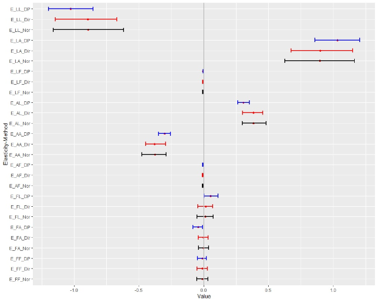
Figure 1: 95% hpdi’s of Price Elasticities of the U.S. Banks’ Factor Demands

Note: We present all nine elasticities (e.g. “E_FA” for the elasticity of funding w.r.t. the asset price) estimated with the three estimators: dp-sur, dir-sur and nor-sur. The three estimators are also allocated with the colours blue, red and black in the same order.

Figure 2: Histograms of the Elasticity of Funding w.r.t. Asset Price, U.S. Banks

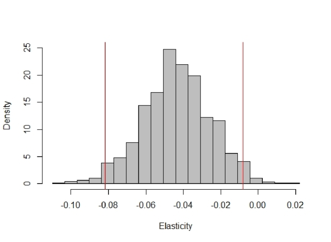
(a) dp-sur

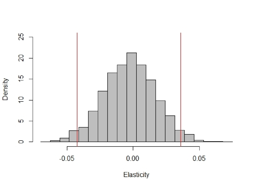
(b) dir-sur

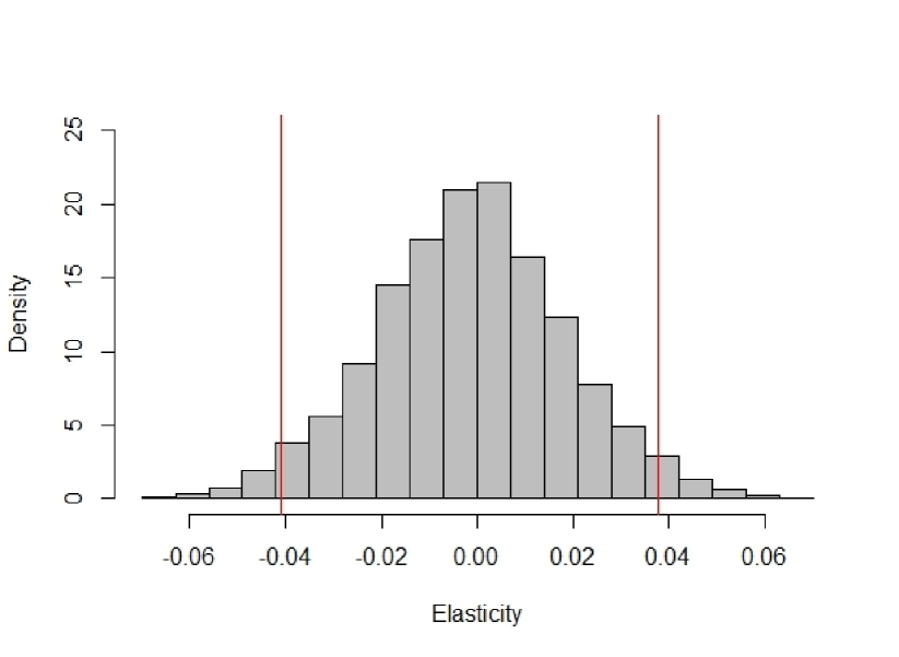
(c) nor-sur

Note: The three panels (2(a)), (2(b)) and (2(c)) are the histograms of the posterior draws for the elasticity of funding w.r.t. the price of assets by dp-sur, dir-sur and nor-sur, respectively. The two vertical lines (in red colour) mark the lower and upper bounds of the 95% hpdi’s, which are $(-0.0818,-0.0082)$ for dp-sur, $(-0.0424,0.0360)$ for dir-sur, and $(-0.0408,0.0379)$ for nor-sur.

We also present the histograms of $E_{FA}$ to further demonstrate the performance of the three estimators in Figure 2. One may see that only the dp-sur gives such an hpdi that excludes 0. From the histogram one may also see that the posterior given by our dp-sur is left skewed with the non-parametric mixture. In fact, the posterior mode of the number of clusters is 3, showing that heterogeneity is detected in the error distributions.

In Figure 3 we present the posterior means of predictive densities of the residuals obtained by the dp-sur and nor-sur. One may see that with the semi-parametric dp-sur, the predictive density of the residuals is bi-modal, which is not captured by the nor-sur.

Figure 3: Predictive Densities of Residuals, U.S. Banks

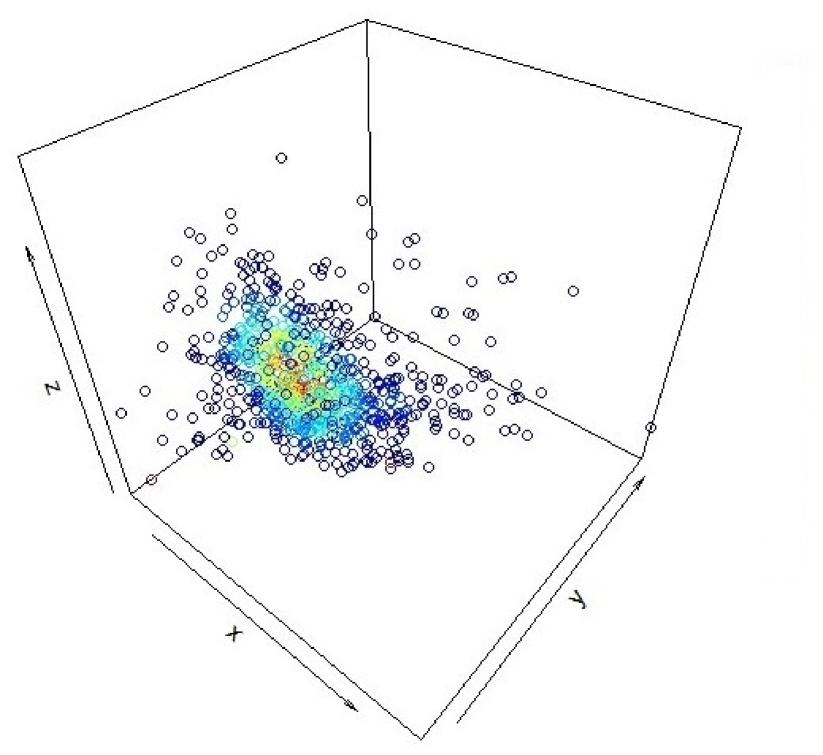
(a) dp-sur

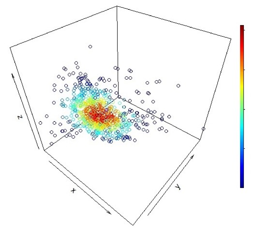
(b) nor-sur

Note: As there are three equations in the system, each residual is a 3 by 1 vector, which is represented by a circle in the 3D coordinate system. The x, y and z axes represent the residuals in the labour ($L$), assets ($A$) and funding ($F$) equations in (30), respectively. Predictive densities of the residuals are reflected in the colours of the circles. The circle colours change from blue to red with higher predictive densities of the corresponding residuals. Panels 3(a) and 3(b) show the residuals of dp-sur and nor-sur, respectively.

4 Semi-parametric Approach to Random Effects Model

The gls has also seen numerous applications with panel data models, and in particular the random effects model (rem). In a panel with $N$ units and $T$ time periods, the error of each unit is a $T\times 1$ vector. We will relax the assumption of parametric Bayesian gls for the rem (Koop, 2003) that the error vectors for all units have the same distribution. In this section we propose a semi-parametric Bayesian approach by introducing $\mathcal{DP}$ priors on the distributional parameters of the random effects and idiosyncratic errors. We follow the same approach as in the dp-sur method in terms of applying the $\mathcal{DP}$ prior on the distributional parameters.

Consider the following panel data model

$$y_{it}=\beta_{1}x_{1it}+\cdots+\beta_{K}x_{Kit}+u_{i}+\eta_{it}=\bm{x}_{it}^{\prime}\bm{\beta}+\varepsilon_{it},$$ (33)

where $i$ and $t$ index the cross section and time series dimensions of the data, respectively. $y_{it}$ is the dependent variable, $\bm{x}_{it}$ denotes the explanatory variables, and $\bm{\beta}$ is a conformable vector of parameters. $u_{i}$ is the time-invariant unobservable of unit $i$, and $\eta_{it}$ the idiosyncratic error term. $\varepsilon_{it}=u_{i}+\eta_{it}$ is the composite error.

In Bayesian methods the difference between the fixed and random effects lies in the choice of prior for the individual effects $u_{i}$: the fixed effects model assumes a non-hierarchical prior for $u_{i}$; and the rem includes a hierarchical prior. The prior for $u_{i}$ in the rem can be written as

$$u_{i}|\mu_{u},\sigma_{u}^{2}\overset{iid}{\sim}\mathcal{N}\left(\mu_{u},\sigma_{u}^{2}\right),$$ (34)

where $\mu_{u}$ and $\sigma_{u}^{2}$ are the mean and variance of $u_{i}$, respectively. Assuming $\eta_{it}\overset{iid}{\sim}\mathcal{N}(\mu_{\eta},\sigma_{\eta}^{2})$, the likelihood of $\bm{\beta}$ marginalized over $u_{i}$ in the Bayesian rem may be written as

$$p\left(\bm{y}_{i}|\bm{\beta},\mu,\bm{\Sigma}\right)=\frac{1}{(2\pi)^{T/2}}|\bm{\Sigma}|^{-\frac{1}{2}}\mathrm{exp}\left[-\frac{1}{2}(\bm{y}_{i}-\bm{X}_{i}\bm{\beta}-\mu\iota_{T})^{\prime}\bm{\Sigma}(\bm{y}_{i}-\bm{X}_{i}\bm{\beta}-\mu\iota_{T})\right],$$ (35)

where $\bm{X}_{i}=\left[x_{1it},\ldots,x_{Kit}\right]_{t=1}^{T}$ is a $T\times K$ matrix of explanatory variables, and $\bm{y}_{i}=[y_{it}]_{t=1}^{T}$ is a $T\times 1$ vector of dependent variables. $\mu=\mu_{u}+\mu_{\eta}$ is the mean of the composite error $\varepsilon_{it}$, and $\iota_{T}$ is a $T\times 1$ vector of ones. $\bm{\Sigma}$ is the covariance matrix of the $T\times 1$ composite error vector $\bm{\varepsilon}_{i}=[\varepsilon_{i1},\varepsilon_{i2},\ldots,\varepsilon_{iT}]^{\prime}$. Assuming the usual strict exogeneity in rem, $\bm{\Sigma}$ is

$$\bm{\Sigma}=\sigma_{\eta}^{2}\bm{I}_{T}+\sigma_{u}^{2}\iota_{T}\iota^{\prime}_{T}=\begin{bmatrix}\sigma_{\eta}^{2}+\sigma_{u}^{2}&\sigma_{u}^{2}&\cdots&\sigma_{u}^{2}\\ \sigma_{u}^{2}&\sigma_{\eta}^{2}+\sigma_{u}^{2}&\cdots&\sigma_{u}^{2}\\ \vdots&\vdots&\ddots&\vdots\\ \sigma_{u}^{2}&\sigma_{u}^{2}&\cdots&\sigma_{\eta}^{2}+\sigma_{u}^{2}\\ \end{bmatrix}.$$ (36)

4.1 DP Prior for REM

In this paper our primary focus is the provision of more efficient inference by exploiting information in the heterogeneous distributions of unobservables. Thus, we maintain the approach of gls, and focus on heterogeneity in the distributional parameters of the unobservables instead of introducing heterogeneity to the distribution of model parameters themselves. In this sense, our method is in the same spirit as the literature pioneered by Conley et al. (2008). We relax the identical distribution assumptions for both $\eta_{it}$ and $u_{i}$ by introducing two independent $\mathcal{DP}$ priors on their distributional parameters.

The $\mathcal{DP}$ prior for $\theta_{\eta,it}=(\mu_{\eta,it},\sigma^{2}_{\eta,it})$, the parameters of the idiosyncratic error $\eta_{it}$, is

$$G \sim\mathcal{DP}\left(\alpha_{\eta},G_{0}\right)$$ (37)

$$\theta_{\eta,it}|G \sim G,$$

where $\alpha_{\eta}$ and $G_{0}$ denote the concentration parameter and base distribution of the $\mathcal{DP}$ prior, respectively. As the prior is introduced across all idiosyncratic errors, the grouping of distributional parameters $\theta_{\eta,it}$ are not restricted to either within the cross section or within the time series dimensions. This means $\eta_{it}$ and $\eta_{is}$ can be allocated to different groups $c_{it}$ and $c_{is}$ such that they have different distributions with parameters $\theta_{\eta,c_{it}}^{*}=(\mu_{\eta,c_{it}}^{*},\sigma_{\eta,c_{it}}^{2*})$ and $\theta_{\eta,c_{is}}^{*}=(\mu_{\eta,c_{is}}^{*},\sigma_{\eta,c_{is}}^{2*})$, respectively. Similarly, $\eta_{it}$ and $\eta_{jt}$ can be in the same group, i.e., $c_{it}=c_{jt}$, making them identically distributed with parameters $\theta_{\eta,c_{it}}^{*}=\theta_{\eta,c_{jt}}^{*}$.

We write the $\mathcal{DP}$ prior for $\theta_{u,i}=(\mu_{u,i},\sigma^{2}_{u,i})$, the parameters of the individual effects $u_{i}$’s, as

$$F \sim\mathcal{DP}\left(\alpha_{u},F_{0}\right)$$ (38)

$$\theta_{u,i}|F \sim F,$$

where $\alpha_{u}$ is the concentration parameter, and $F_{0}$ is the base distribution of the $\mathcal{DP}$ prior. Given that we maintain the assumption of strictly exogeneity of rem, it is reasonable to introduce a $\mathcal{DP}$ prior independent of $G$ for the distributional parameters $\theta_{u,i}$.

The $\mathcal{DP}$ prior on the distributional parameters of individual effects $u_{i}$ generates groupings across the $N$ units. As a result, if $u_{i}$ and $u_{j}$ are in different groups $c_{i}$ and $c_{j}$, their parameters will take the values $\theta_{u,c_{i}}^{*}=(\mu_{u,c_{i}}^{*},\sigma_{u,c_{i}}^{2*})$ and $\theta_{u,c_{j}}^{*}=(\mu_{u,c_{j}}^{*},\sigma_{u,c_{j}}^{2*})$, respectively. This relaxes the rem assumption that the individual effects are identically distributed, as $u_{i}$ and $u_{j}$ are allowed to have different distributional parameters.

The mean vector of the composite error vector $\bm{\varepsilon}_{i}=u_{i}\iota+\bm{\eta}_{i}$ is then given by

$$\bm{\mu}_{i}=\mu_{u,c_{i}}^{*}\iota_{T}+\bm{\mu}_{\bm{\eta}_{i}}=\mu_{u,c_{i}}^{*}\iota_{T}+\begin{bmatrix}\mu_{\eta,c_{i1}}^{*},\ldots,\mu_{\eta,c_{iT}}^{*}\end{bmatrix}^{\prime},$$ (39)

where $\bm{\mu}_{\bm{\eta}_{i}}$ is the mean vector of $\bm{\eta}_{i}$. The covariance matrix of $\bm{\varepsilon}_{i}$ is

$$\bm{\Sigma}_{i}=\bm{\Sigma}_{\bm{\eta}_{i}}+\sigma_{u,c_{i}}^{2*}\iota_{T}\iota^{\prime}_{T}=\mathbf{diag}\left(\sigma_{\eta,c_{i1}}^{2*},\ldots,\sigma_{\eta,c_{iT}}^{2*}\right)+\sigma_{u,c_{i}}^{2*}\iota_{T}\iota^{\prime}_{T},$$ (40)

where $\bm{\Sigma}_{\bm{\eta}_{i}}=\mathbf{diag}\left(\sigma_{\eta,c_{i1}}^{2*},\ldots,\sigma_{\eta,c_{iT}}^{2*}\right)$ is the diagonal covariance matrix of $\bm{\eta}_{i}$, where the diagonal elements are the variances of the idiosyncratic errors of unit $i$ over all time periods.

The mcmc algorithm utilised to draw from the posterior distributions is similar to that described in Section 2.3 with a few minor changes due to the particular form of the dp-rem. The most significant change is that now the individual effects $\bm{U}=\{u_{i}\}_{i=1}^{N}$ must also be drawn. In addition, there are two sets of distributional parameters, i.e., $\Theta_{u}$ and $\Theta_{\eta}$ for $u_{i}$ and $\eta_{it}$, respectively. Similarly, there are concentration parameters for the two independent $\mathcal{DP}$ priors, namely $\alpha_{u}$ and $\alpha_{\eta}$. Accordingly, the Gibbs sampler consists of

$$\Theta_{\eta} |\bm{y},\bm{X},U,\bm{\beta},\Theta_{u},\alpha_{u},\alpha_{\eta}$$ (41)

$$\Theta_{u} |\bm{y},\bm{X},U,\bm{\beta},\Theta_{\eta},\alpha_{u},\alpha_{\eta}$$

$$U |\bm{y},\bm{X},\bm{\beta},\Theta_{u},\Theta_{\eta},\alpha_{u},\alpha_{\eta}$$

$$\bm{\beta} |\bm{y},\bm{X},U,\Theta_{u},\Theta_{\eta},\alpha_{u},\alpha_{\eta}$$

$$\alpha_{u} |\bm{y},\bm{X},U,\bm{\beta},\Theta_{u},\Theta_{\eta},\alpha_{\eta}$$

$$\alpha_{\eta} |\bm{y},\bm{X},U,\bm{\beta},\Theta_{u},\Theta_{\eta},\alpha_{u}.$$

Among the parameters, the drawing of the concentration parameters $\alpha_{u}$ and $\alpha_{\eta}$ is exactly the same as described in Section 2.3, because the two $\mathcal{DP}$ priors in our dp-rem are independent. The drawing of $\Theta_{u}$ and $\Theta_{\eta}$ are also similar to the procedure described in (12) to (17). It should be noted that the normal-inverse Wishart distribution in (10) can still serve as the base distributions $G_{0}$ and $F_{0}$. However, as both $u_{i}$ and $\eta_{it}$ are scalars, they become the normal-inverse gamma distribution with both $\bm{\lambda}_{0}$ and $\bm{W}_{0}$ being scalars consequently.

The drawing of $\bm{U}$ is based on the fact that for a given $i$, the hierarchical prior for $u_{i}$ is

$$u_{i}|\mu_{u,c_{i}}^{*},\sigma_{u,c_{i}}^{*2}\sim\mathcal{N}\left(\mu_{u,c_{i}}^{*},\sigma_{u,c_{i}}^{*2}\right),$$ (42)

which is the conjugate prior for the normal likelihood, leading to the posterior of $u_{i}$ being normal as well. The posterior variance of $u_{i}$ is

$$s_{i}^{2}=\left(\sigma_{u,c_{i}}^{*-2}+\iota^{\prime}_{T}\bm{\Sigma}_{\bm{\eta}_{i}}^{-1}\iota_{T}\right)^{-1}.$$ (43)

The posterior mean of $u_{i}$ is

$$m_{i}=s_{i}^{2}\left(\sigma_{u,c_{i}}^{*-2}\mu_{u,c_{i}}^{*}+\iota^{\prime}_{T}\bm{\Sigma}_{\bm{\eta}_{i}}^{-1}\left(\bm{y}_{i}-\bm{X}_{i}\bm{\beta}-\bm{\mu}_{\bm{\eta}_{i}}\right)\right).$$ (44)

As for the regression parameter $\bm{\beta}$, its likelihood marginalized over ${u_{i}}$ is given by

$$p\left(\bm{y}_{i}|\bm{\beta},\bm{\mu}_{i},\bm{\Sigma}_{i}\right)=\frac{1}{(2\pi)^{T/2}}|\bm{\Sigma}_{i}|^{-\frac{1}{2}}\exp\left[-\frac{1}{2}\left(\bm{y}_{i}-\bm{X}_{i}\bm{\beta}-\bm{\mu}_{i}\right)^{\prime}\bm{\Sigma}_{i}^{-1}\left(\bm{y}_{i}-\bm{X}_{i}\bm{\beta}-\bm{\mu}_{i}\right)\right],$$ (45)

which differs from (18) only in that $\bm{\mu}_{i}$, the mean of the composite error $\bm{\varepsilon}_{i}$ is included. Compared with the marginal likelihood of the parametric Bayesian rem in (35), the covariance matrix of the composite error vector $\bm{\varepsilon_{i}}$ is allowed to be different for each unit $i$ in the panel.

Given a conjugate normal prior for $\bm{\beta}$, i.e.,

$$\bm{\beta}\sim\mathcal{N}(\bm{b}_{0},\bm{V}_{0}),$$

where $\bm{b}_{0}$ and $\bm{V}_{0}$ respectively denote the prior mean and covariance matrix of $\bm{\beta}$, the posterior covariance matrix of $\bm{\beta}$, marginalized over $u_{i}$, is given by

$$\bm{V}=\left(\bm{V}_{0}^{-1}+\sum_{i=1}^{N}{\bm{X}_{i}^{\prime}\bm{\Sigma}_{i}^{-1}\bm{X}_{i}}\right)^{-1}.$$ (46)

The posterior mean vector is

$$\bm{b}=\bm{V}\left(\bm{V}_{0}^{-1}\bm{b}_{0}+\sum_{i=1}^{N}{\bm{X}_{i}^{\prime}\bm{\Sigma}_{i}^{-1}\left(\bm{y}_{i}-\bm{\mu}_{i}\right)}\right).$$ (47)

A modified version of our dp-rem can be introduced in the spirit of the correlated rem introduced by Mundlak (1978) and further discussed by Chamberlain (1982), Wooldridge (2005), Murtazashvili and Wooldridge (2008) and Wooldridge (2019). This model offers a middle ground between the fixed and random effects models by allowing the individual effects to be correlated with $\bm{X}_{i}$ in a specific manner. This is achieved by specifying the individual effects as a linear function of the within unit means of the explanatory variables, i.e.,

$$y_{it} =\beta_{1}x_{1it}+\cdots+\beta_{K}x_{Kit}+a_{i}+\eta_{it},$$ (48)

$$a_{i} =\gamma_{1}\bar{x}_{1i}+\cdots+\gamma_{K}\bar{x}_{Ki}+u_{i},$$

where $\bar{x}_{ki}=1/T\sum_{t=1}^{T}{x_{kit}}$. Then a $\mathcal{DP}$ prior as in (38) can be applied to $u_{i}$, and the analyses of the parameters are similar.

4.2 DP-REM Simulation Results

We carry out a series of simulation experiments to demonstrate the performance of our dp-rem. Similar to the simulations for the dp-sur, our dp-rem is compared with two other estimators. The first one is a Bayesian rem with a Dirichlet prior on the distributional parameters of $u_{i}$ and $\eta_{it}$ (dir-rem hereafter), where $u_{i}$ and $\eta_{it}$ have parametric mixtures of normal distributions. The second one assumes that $u_{i}$ and $\eta_{it}$ are normal distributed (nor-rem hereafter).

The simulations are carried out using the following specification

$$y_{it}=\beta_{1}x_{1it}+\beta_{2}x_{2it}+u_{i}+\eta_{it},$$ (49)

where the explanatory variables are generated from

$$x_{1it}\sim\mathcal{N}\left(1,1\right),\quad x_{2it}\sim\mathcal{N}\left(3,1\right)$$

with

$$\beta_{1}=5,\ \beta_{2}=-5.$$

The individual effects $u_{i}$ and the idiosyncratic errors $\eta_{it}$ are independently generated. As with the simulation experiments for the dp-sur, we specify two types of distributions: a log-normal distribution and a bi-modal distributions. For the log-normal distribution, the variances of $\ln u_{i}$ and $\ln\eta_{it}$ are chosen to be equal and denoted by $\sigma^{2}$, which are set to three values: 1, 1.5 and 2, in order to explore the performance of our dp-rem under different circumstances.

To create a bi-modal distribution, we mix two non-central univariate t distributions with non-centrality parameters -1 and 4. Like in the experiment design in Section 3.2, the $df$ are set to 2, 4, 6 and $\infty$ to adjust the heaviness of the tails. The weights assigned to the two non-central t distributions are 0.4 and 0.6, so that the mixture distribution is asymmetric.

To explore the performance of our dp-rem estimator with different sample sizes, we fix the number of periods in the panel at 3 and set the number of cross sections to 100, 200 and 300. 100 samples are generated for each sample size, and the results reported in this section are the average over all the samples.

4.2.1 Results with Log-normal Distributions

Table 4 presents the results of the simulations with log-normal distributed individual effects $u_{i}$ and idiosyncratic errors $\eta_{it}$. For the posterior means we observe that the three estimators all perform well. When $\sigma^{2}=2$, we observe the greatest differences for the dir-rem and nor-rem posterior means from the true values. It shows that the two parametric methods are slightly inferior as point estimators when the distributions of $u_{i}$ and $\eta_{it}$ in (49) are more skewed and heavy tailed. This can be caused by the distribution of the composite errors being a convolution of two log-normal distributions, which are fat tailed. The two parametric estimators dir-rem and nor-rem struggle to give good point estimates for the parameters in this case, while our semi-parametric dp-rem uniformly performs well.

Table 4: Simulation Results for REM with Log-normal Distributions

	$N$	100				200				300
	Estimator	DP	DIR	NOR		DP	DIR	NOR		DP	DIR	NOR
	Parameter						$\sigma^{2}=1$
Mean	$\beta_{1}$	5.0094	5.0043	5.0227		4.9905	4.9833	4.9905		4.9998	4.9918	4.9983 [t]
	$\beta_{2}$	-4.9933	-5.0228	-4.9999		-4.9961	-5.0232	-5.0026		-4.9992	-5.0229	-5.0054 [b]
SD	$\beta_{1}$	0.0475	0.1279	0.1311		0.0313	0.0928	0.0941		0.0250	0.0786	0.0799 [t]
	$\beta_{2}$	0.0424	0.1160	0.1229		0.0288	0.0846	0.0893		0.0235	0.0730	0.0758 [b]
MSE	$\beta_{1}$	0.0047	0.0301	0.0362		0.0021	0.0157	0.0181		0.0014	0.0114	0.0131 [t]
	$\beta_{2}$	0.0039	0.0248	0.0291		0.0021	0.0149	0.0172		0.0014	0.0102	0.0122 [b]
							$\sigma^{2}=1.5$
Mean	$\beta_{1}$	5.0034	5.0012	5.0276		5.0015	4.9650	4.9666		4.9947	4.9868	4.9935 [t]
	$\beta_{2}$	-5.0010	-5.0746	-5.0115		-4.9965	-5.0356	-4.9842		-4.9948	-5.0385	-5.0001 [b]
SD	$\beta_{1}$	0.0498	0.2120	0.2273		0.0348	0.1670	0.1806		0.0251	0.1266	0.1337 [t]
	$\beta_{2}$	0.0473	0.1905	0.2178		0.0303	0.1408	0.1605		0.0230	0.1163	0.1282 [b]
MSE	$\beta_{1}$	0.0055	0.0878	0.1254		0.0028	0.0471	0.0686		0.0013	0.0259	0.0345 [t]
	$\beta_{2}$	0.0055	0.0758	0.1121		0.0022	0.0368	0.0596		0.0012	0.0273	0.0336 [b]
							$\sigma^{2}=2$
Mean	$\beta_{1}$	4.9962	4.9449	5.0006		5.0103	4.9520	4.9802		4.9982	4.9382	4.9341 [t]
	$\beta_{2}$	-4.9927	-5.1079	-5.0329		-4.9952	-5.1090	-5.0282		-4.9996	-5.0779	-4.9864 [b]
SD	$\beta_{1}$	0.0524	0.3312	0.3909		0.0342	0.2478	0.2999		0.0259	0.2039	0.2438 [t]
	$\beta_{2}$	0.0467	0.2907	0.3735		0.0296	0.2091	0.2714		0.0232	0.1786	0.2284 [b]
MSE	$\beta_{1}$	0.0058	0.1911	0.4124		0.0029	0.1035	0.2028		0.0012	0.0725	0.1296 [t]
	$\beta_{2}$	0.0050	0.1561	0.2932		0.0019	0.0980	0.1878		0.0012	0.0635	0.1121 [b]

The posterior standard deviations of all three estimators decrease as the sample size increases for all three values of $\sigma^{2}$. Among them, the dp-rem posterior standard deviations are always smaller than dir-rem and nor-rem ones. This indicates that the semi-parametric dp-rem provides posterior distributions that are less dispersed than the two parametric methods, as a result of the non-parametric mixture of normal distributions. It can also be seen that the posterior standard deviations of our dp-rem remains similar when $\sigma^{2}$ increases for any given sample size. In comparison, the posterior standard deviations of the two parametric estimators increase considerably when $\sigma^{2}$ gets larger.

The mse for the dp-rem are always smaller than their dir-rem and nor-rem counterparts. The superior performance of the dp-rem demonstrates the advantage of the non-parametric mixture with the $\mathcal{DP}$ prior over the parametric mixture using the Dirichlet prior, and the homogeneous normal errors. As with the posterior standard deviations, the mse of the dp-rem remain similar when $\sigma^{2}$ increases, while the dir-rem and nor-rem ones increase considerably. This further demonstrates the superiority of our semi-parametric dp-rem when the individual effects and idiosyncratic errors have fat tailed distributions.

4.2.2 Results with Mixed t Distributions

Table 5 reports the results with mixed t distributed individual effects and idiosyncratic errors. It can be seen that for all three estimators their posterior means are close to the truth in all settings. That is, all three estimators perform well as point estimators.

Table 5: Simulation Results for REM with Mixed t Distributions

	$N$	100				200				300
	Estimator	DP	DIR	NOR		DP	DIR	NOR		DP	DIR	NOR
	Parameter						$df=2$
Mean	$\beta_{1}$	4.9958	5.0267	5.0215		4.9894	5.0021	5.0209		4.9939	5.0195	5.0251 [t]
	$\beta_{2}$	-4.9824	-4.9424	-4.9473		-5.0018	-5.0058	-5.0226		-5.0022	-5.0164	-5.0128 [b]
S.D.	$\beta_{1}$	0.0974	0.1777	0.1996		0.0679	0.1300	0.1583		0.0548	0.1036	0.1181 [t]
	$\beta_{2}$	0.0869	0.1632	0.1881		0.0611	0.1190	0.1521		0.0544	0.1079	0.1263 [b]
MSE	$\beta_{1}$	0.0216	0.0522	0.0940		0.0096	0.0270	0.0576		0.0067	0.0185	0.0337 [t]
	$\beta_{2}$	0.0164	0.0494	0.0838		0.0081	0.0236	0.0584		0.0068	0.0190	0.0360 [b]
							$df=4$
Mean	$\beta_{1}$	4.9982	4.9865	4.9869		4.9972	4.9886	4.9894		4.9945	4.9995	4.9993 [t]
	$\beta_{2}$	-5.0186	-5.0254	-5.0274		-5.0047	-5.0051	-5.0051		-5.0021	-5.0084	-5.0082 [b]
S.D.	$\beta_{1}$	0.0855	0.1022	0.1013		0.0624	0.0756	0.0749		0.0464	0.0561	0.0558 [t]
	$\beta_{2}$	0.0715	0.0915	0.0915		0.0540	0.0701	0.0701		0.0453	0.0593	0.0595 [b]
MSE	$\beta_{1}$	0.0147	0.0177	0.0178		0.0094	0.0116	0.0114		0.0036	0.0053	0.0055 [t]
	$\beta_{2}$	0.0122	0.0167	0.0179		0.0073	0.0099	0.0101		0.0048	0.0081	0.0082 [b]
							$df=6$
Mean	$\beta_{1}$	5.0077	5.0118	5.0113		5.0035	5.0005	5.0000		5.0023	5.0026	5.0025 [t]
	$\beta_{2}$	-4.9980	-4.9982	-4.9987		-5.0019	-5.0040	-5.0043		-5.0026	-5.0044	-5.0042 [b]
S.D.	$\beta_{1}$	0.0758	0.0843	0.0836		0.0530	0.0591	0.0584		0.0469	0.0530	0.0528 [t]
	$\beta_{2}$	0.0730	0.0875	0.0871		0.0531	0.0643	0.0638		0.0402	0.0485	0.0483 [b]
MSE	$\beta_{1}$	0.0108	0.0124	0.0123		0.0053	0.0063	0.0062		0.0046	0.0059	0.0059 [t]
	$\beta_{2}$	0.0128	0.0161	0.0160		0.0067	0.0082	0.0082		0.0036	0.0047	0.0048 [b]
							$df=\infty$
Mean	$\beta_{1}$	5.0003	5.0006	5.0005		5.0000	5.0046	5.0047		4.9941	4.9943	4.9944 [t]
	$\beta_{2}$	-4.9987	-4.9942	-4.9943		-4.9946	-4.9991	-4.9991		-4.9991	-5.0015	-5.0014 [b]
S.D.	$\beta_{1}$	0.0695	0.0741	0.0738		0.0452	0.0478	0.0477		0.0389	0.0417	0.0416 [t]
	$\beta_{2}$	0.0661	0.0763	0.0761		0.0438	0.0505	0.0505		0.0348	0.0398	0.0397 [b]
MSE	$\beta_{1}$	0.0087	0.0097	0.0097		0.0042	0.0047	0.0047		0.0032	0.0036	0.0036 [t]
	$\beta_{2}$	0.0093	0.0111	0.0111		0.0038	0.0045	0.0045		0.0027	0.0032	0.0032 [b]

The posterior standard deviations of our dp-rem are the smallest in all scenarios, indicating that its posteriors are more concentrated than the dir-rem and nor-rem ones. We also observe that for a given sample size the advantages of the dp-rem over the parametric dir-rem and nor-rem with respect to posterior standard deviations are the largest when $df=2$, and become smaller as $df$ increases. This is the result of the tails of the t distributions mixed in the error distributions becoming less heavy. In addition, the dir-rem gives almost the same posterior standard deviations as the nor-rem when $df$ are 4, 6 and $\infty$. This demonstrates that the advantages of the dp-rem over the dir-rem and nor-rem fall at a slower rate than that of the dir-rem over the nor-rem when $df$ increases.

Our dp-rem dominates the two parametric estimators regarding mse under all circumstances. Similar to the posterior standard deviations, the advantages of the dp-rem over the dir-rem and nor-rem in terms of mse fall as the $df$ increases, as the tails of the mixed t distributions become less heavy. It should be noted that the mse of dir-rem and nor-rem are almost identical when $df=4$. That is, the advantage of the dir-rem over the nor-rem has diminished. In contrast, the advantage of the dp-rem over the two parametric estimators is still present. This demonstrates that the parametric dir-rem and nor-rem are not as good as the semi-parametric dp-rem at identifying the heterogeneity in error distributions when the tails become less heavy.

4.3 DP-REM Empirical Examples

As a demonstration of the dp-rem with real data, in this section we present the results regarding a model for wages of U.S. workers. The data are from Cornwell and Rupert (1988) with 595 individuals over a period of 7 years, from 1976 to 1982. In fact, it allows us to demonstrate the correlated rem in (48), as outlined below. The model is given by

$$\text{ln}Wage_{it}=\beta_{1}Exp_{it}+\beta_{2}Mar_{it}+\beta_{3}Fem_{i}+\beta_{4}Edu_{it}+v_{i}+\varepsilon_{it},$$ (50)

where the dependent variable is the logarithms of wages, and the explanatory variables are experience in years ($Exp$), dummies for marriage status ($Mar$) and the individual being female ($Fem$), as well as the years of education ($Edu$). As there are strong reasons to suspect that the unobserved individual effect $v_{i}$ is correlated with the explanatory variables due to omitted variables such as ability and motivation, the correlated rem is selected. It specifies $v_{i}$ as

$$v_{i}=\tilde{\beta_{1}}AExp_{i}+\tilde{\beta_{2}}AMar_{i}+u_{i},$$ (51)

where the sample averages of experience ($AExp$) and marriage status ($AMar$) of individual $i$ are included, as they are the two time variant variables in (50). The posterior means, standard deviations and p-values of the parameters with the three estimators dp-rem, dir-rem and nor-rem are presented in Table 6. We also demonstrate their respective performances with a number of figures.

From Table 6 we observe that the posterior means are similar for all parameters. Among the explanatory variables, experience and education are positively correlated with workers’ wages, while being married and female negatively influences wages. The semi-parametric dp-rem gives the smallest posterior standard deviations among all three estimators. As the posterior modes of the numbers of clusters for $u_{i}$ and $\varepsilon_{i}$ are 2 and 6, respectively, heterogeneity is detected in both the individual effects’ and the idiosyncratic errors’ distributions. The posterior p-values of the dp-rem are also the smallest for all parameters. It should be noted that both parameters in (51) have posterior p-values less than 5%, indicating that $v_{i}$ are correlated with the explanatory variables, providing support for the application of the correlated rem.

Table 6: U.S. Individual Wage

		Mean				SD				p-values
Parameter	DP	Dir	Nor		DP	Dir	Nor		DP	Dir	Nor
$Exp$	0.0912	0.0968	0.0969		0.0007	0.0013	0.0013		0.0000	0.0000	0.0000
$Mar$	-0.0194	-0.0323	-0.0324		0.0114	0.0197	0.0216		0.0880	0.0920	0.1520
$Fem$	-0.3259	-0.3160	-0.3110		0.0592	0.0639	0.0777		0.0000	0.0000	0.0000
$Edu$	0.0771	0.0731	0.0738		0.0041	0.0048	0.0049		0.0000	0.0000	0.0000
$AExp$	-0.0823	-0.0885	-0.0885		0.0015	0.0018	0.0020		0.0000	0.0000	0.0000
$AMar$	0.1578	0.1796	0.1850		0.0521	0.0602	0.0697		0.0000	0.0020	0.0080

In Figure 4 we present the 95% hpdi’s of the three estimators for all regression parameters in (51). One can observe that the semi-parametric dp-rem yields the narrowest 95% hpdi’s for all parameters, followed by the dir-rem with a parametric mixture. The parametric nor-rem has the widest hpdi’s for all the parameters, though for some parameters its hpdi’s are rather similar to those of dir-rem, e.g. with the parameter $\beta_{4}$ for education.

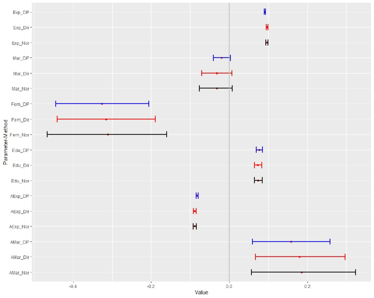
Figure 4: 95% hpdi’s of Parameters in the U.S. Wage Model

Note: For the parameter of each variable (e.g. “Edu” for education), we present the 95% HPDI’s of all three estimators: dp-rem, dir-rem and nor-rem. The three estimators are also allocated with the colours blue, red and black in the same order.

Figure 5 presents the histograms of the posterior draws for the education parameter ($\beta_{4}$). Though all three intervals exclude zero, the dp-rem one is the shortest, as a result of the efficiency gain from exploring the heterogeneity in the error distributions.

Figure 5: Histograms of the Parameter for Education

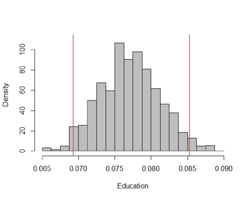
(a) dp-rem

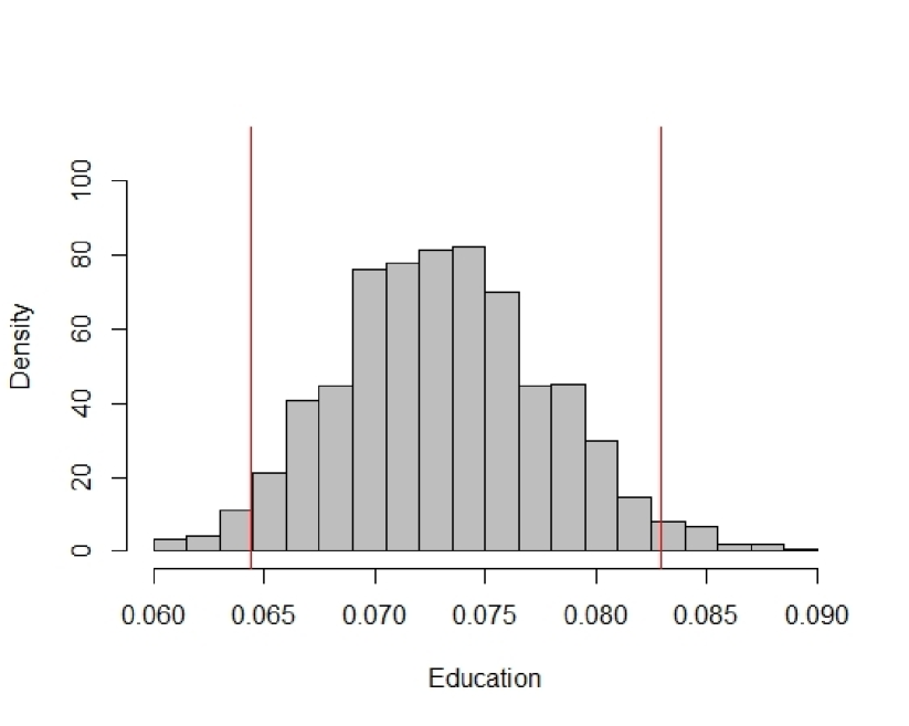
(b) dir-rem

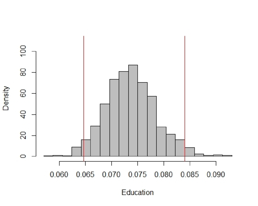
(c) nor-rem

Note: The three panels (5(a)), (5(b)) and (5(c)) are for the dp-rem, dir-rem and nor-rem, respectively. The interval is $(0.0692,0.0852)$ for dp-rem, $(0.0643,0.0829)$ for dir-rem, and $(0.0646,0.0840)$ for nor-rem. The lower and upper bounds of the 95% hpdi’s are marked by (red) vertical lines.

Figure 6 presents the predictive densities of the fitted individual effects and residuals obtained by the semi-parametric dp-rem and the parametric nor-rem, respectively. One can see that both the fitted individual effects and the residuals have multi-modal distributions with our dp-rem, which is not captured by the nor-rem. Thus, the normal distribution assumption could cause potential losses in efficiency.

Figure 6: Predictive Densities of Individual Effects and Residuals

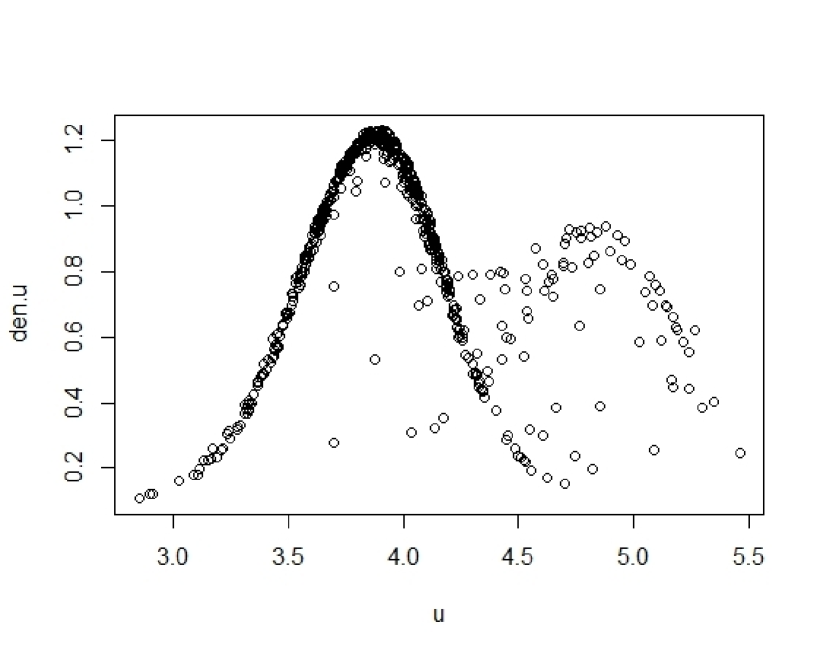
(a) u, dp-rem

(b) u, nor-rem

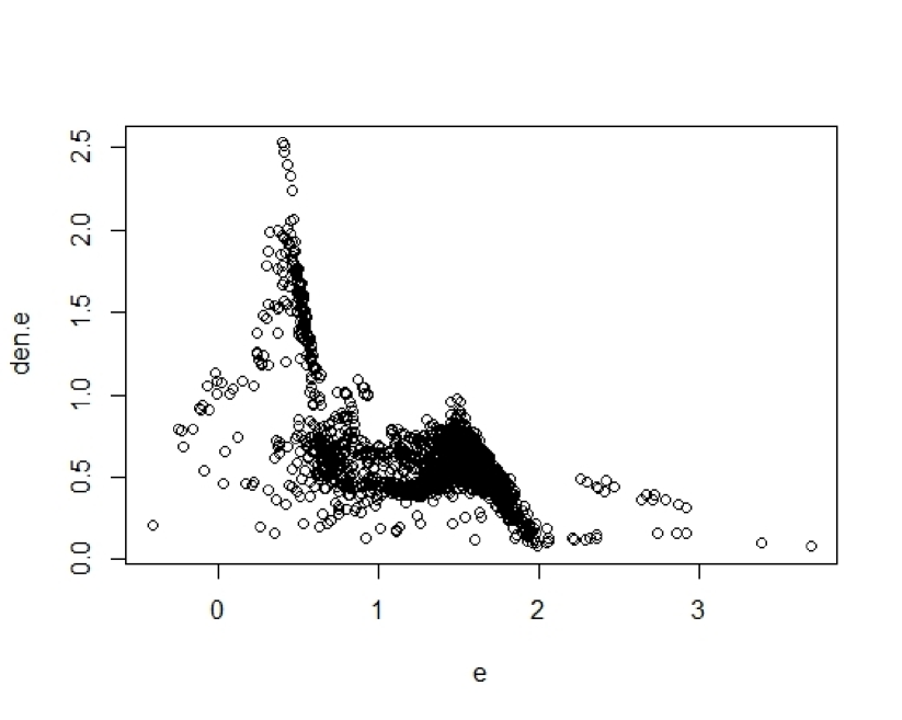
(c) e, dp-rem

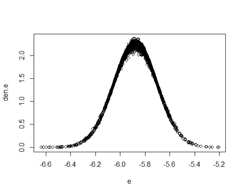
(d) e, nor-rem

Note: The predictive densities of the individual effects are in panels (6(a)) (dp-rem) and (6(b)) (nor-rem). The predictive densities of the residuals are in panel (6(c)) (dp-rem) and (6(d)) (nor-rem).

5 Conclusion

In this paper we address the potential violation of the assumptions made by parametric Bayesian gls estimators that the errors are homogeneous regarding their distributions. Such assumptions are likely to be problematic in reality particularly when micro data are used, as the features of individuals or households are likely to lead to observations having different distributions. We present a semi-parametric Bayesian gls where the error distribution is a non-parametric mixture of normal distributions by introducing a Dirichlet process prior on the distributional parameters of the errors. The number of normal components is decided jointly by the data and the prior in such a mixture, which is able to cover a large variety of distributions. The errors are grouped by the $\mathcal{DP}$ prior, with those in the same group having the same distributional parameters and thus the same distribution. Two specific cases of the semi-parametric Bayesian gls are then introduced, which are the sur for equation systems and the rem for panel data.

Our dp-sur and dp-rem methods are demonstrated with a series of simulation experiments consisting of two scenarios, where the errors have a log-normal distribution and a mixture of t distributions that are bi-modal and asymmetric, respectively. When the errors have a log-normal distribution, which is fat tailed, our semi-parametric gls estimator gives smaller posterior standard deviations, as well as smaller mean squared errors in all settings. Such advantages over the parametric estimators are greater when the variances of the errors are larger, leading to heavier tails of the error distributions. When the errors are bi-modal as a mixture of t distributions, our semi-parametric gls estimators also out-perform the parametric estimators with respect to posterior standard errors and mean squared errors in all scenarios. Such advantages are larger when the degrees of freedom of the t mixture components are smaller, i.e., the tails of the mixture are heavier.

We apply our dp-sur method to the demands for production factors with the generalized Leontief cost function using a dataset of the U.S. banking industry. Heterogeneity is detected in the sample by our semi-parametric estimator. The dp-sur posterior standard deviations are smaller than the dir-sur ones using a parametric mixture of normal distributions, as well as the nor-sur ones for all the demand elasticities. In addition, the posterior p-values of the dp-sur are also smaller for all the parameters.

Our dp-rem is also applied to a study U.S. workers’ wages, where there is a strong reason to suspect that the unobserved individual effects are correlated with the explanatory variables due to omitted variables describing individual features such as abilities. The correlated rem is then estimated. The dp-rem detects heterogeneity in the distributions of both the individual effects and the idiosyncratic errors with this sample. Our dp-rem obtains smaller posterior standard deviations and p-values than the parametric dir-rem and nor-rem for all parameters.

References

- [1] Aldous, D. J. (1985). Exchangeability and related topics. In École d’Été de Probabilités de Saint-Flour XIII—1983. Springer, Berlin, 1-198.
- [2] Allenby, G. M., Arora, N., & Ginter, J. L. (1998). On the heterogeneity of demand. Journal of Marketing Research, 384-389.
- [3] Andrews, D. F., & Mallows, C. L. (1974). Scale mixtures of normal distributions. Journal of the Royal Statistical Society. Series B (Methodological), 99-102.
- [4] Antoniak, C. E. (1974). Mixtures of Dirichlet processes with applications to Bayesian nonparametric problems. The Annals of Statistics, 1152-1174.
- [5] de Carvalho, V. I., Jara, A., Hanson, T. E., & de Carvalho, M. (2013). Bayesian nonparametric ROC regression modeling. Bayesian Analysis, 8(3), 623-646.
- [6] Chamberlain, G. (1982). Multivariate regression models for panel data. Journal of econometrics, 18(1), 5-46.
- [7] Chao, J. C., & Phillips, P. C. (1998). Posterior distributions in limited information analysis of the simultaneous equations model using the Jeffreys prior. Journal of Econometrics, 87(1), 49-86.
- [8] Chigira, H., & Shiba, T. (2015). Dirichlet Prior for Estimating Unknown Regression Error Heteroskedasticity. TERG Discussion Papers, 341, 1-17.
- [9] Conley, T. G., Hansen, C. B., McCulloch, R. E., & Rossi, P. E. (2008). A semi-parametric Bayesian approach to the instrumental variable problem. Journal of Econometrics, 144(1), 276-305.
- [10] Cornwell, C., & Rupert, P. (1988). Efficient estimation with panel data: An empirical comparison of instrumental variables estimators. Journal of Applied Econometrics, 3(2), 149-155.
- [11] Diewert, W. E. (1971). An application of the Shephard duality theorem: a generalized Leontief production function. Journal of Political Economy, 79(3), 481-507.
- [12] Escobar, M. D., & West, M. (1995). Bayesian density estimation and inference using mixtures. Journal of the american statistical association, 90(430), 577-588.
- [13] Escobar, M. D., & West, M. (1998). Computing nonparametric hierarchical models. In: Dey, D., MüIler, P., & Sinha, D. Practical nonparametric and semiparametric Bayesian statistics. Springer, New York, 1-22.
- [14] Ferguson, T. S. (1973). A Bayesian analysis of some nonparametric problems. The Annals of Statistics, 1(2), 209-230.
- [15] Gershman, S. J., & Blei, D. M. (2012). A tutorial on Bayesian nonparametric models. Journal of Mathematical Psychology, 56(1), 1-12.
- [16] Geweke, J. (1993). Bayesian treatment of the independent student‐t linear model. Journal of Applied Econometrics, 8(S1).
- [17] Geweke, J. (1996). Bayesian reduced rank regression in econometrics. Journal of Econometrics, 75(1), 121-146.
- [18] Hejblum, B. P., Alkhassim, C., Gottardo, R., Caron, F., & Thiébaut, R. (2019). Sequential Dirichlet process mixtures of multivariate skew -distributions for model-based clustering of flow cytometry data. The Annals of Applied Statistics, 13(1), 638-660.
- [19] Hirano, K. (2002). Semiparametric Bayesian inference in autoregressive panel data models. Econometrica, 70(2), 781-799.
- [20] Kleinman, K. P., & Ibrahim, J. G. (1998). A semiparametric Bayesian approach to the random effects model. Biometrics, 921-938.
- [21] Kleibergen, F., & van Dijk, H. K. (1998). Bayesian simultaneous equations analysis using reduced rank structures. Econometric Theory, 14(6), 701-743.
- [22] Koop, G. (2003). Bayesian Econometrics. John Wiley & Sons.
- [23] Kyung, M., Gill, J., & Casella, G. (2010). Estimation in Dirichlet random effects models. The Annals of Statistics, 38(2), 979-1009.
- [24] Li, M., & Tobias, J. L. (2011). Bayesian inference in a correlated random coefficients model: Modeling causal effect heterogeneity with an application to heterogeneous returns to schooling. Journal of econometrics, 162(2), 345-361.
- [25] Li, C., Casella, G., & Ghosh, M. (2018). Estimation of regression vectors in linear mixed models with Dirichlet process random effects. Communications in Statistics-Theory and Methods, 47(16), 3935-3954.
- [26] MacEachern, S. N. (1998). Computational methods for mixture of Dirichlet process models. In: Dey, D., MüIler, P., & Sinha, D. Practical nonparametric and semiparametric Bayesian statistics. Springer, New York, 23-43.
- [27] Malikov, E., Kumbhakar, S. C., & Tsionas, M. G. (2016). A cost system approach to the stochastic directional technology distance function with undesirable outputs: the case of US banks in 2001-2010. Journal of Applied Econometrics, 31(7), 1407-1429.
- [28] Mundlak, Y. (1978). On the pooling of time series and cross section data. Econometrica: journal of the Econometric Society, 46(1978), 69-85.
- [29] Murtazashvili, I., & Wooldridge, J. M. (2008). Fixed effects instrumental variables estimation in correlated random coefficient panel data models. Journal of Econometrics, 142(1), 539-552.
- [30] Rossi, P. E., Allenby, G. M., & McCulloch, R. (2012). Bayesian statistics and marketing. John Wiley & Sons.
- [31] Teh, Y. W., Jordan, M. I., Beal, M. J., & Blei, D. M. (2005). Sharing clusters among related groups: Hierarchical Dirichlet processes. In Advances in neural information processing systems (pp. 1385-1392).
- [32] Teh, Y. W. (2011). Dirichlet Process. In Encyclopedia of machine learning, pp. 280-287. Springer US.
- [33] Wiesenfarth, M., Hisgen, C. M., Kneib, T., & Cadarso-Suarez, C. (2014). Bayesian nonparametric instrumental variables regression based on penalized splines and dirichlet process mixtures. Journal of Business & Economic Statistics, 32(3), 468-482.
- [34] Wooldridge, J. M. (2003). Cluster-sample methods in applied econometrics. American Economic Review, 93(2), 133-138.
- [35] Wooldridge, J. M. (2005). Fixed-effects and related estimators for correlated random-coefficient and treatment-effect panel data models. Review of Economics and Statistics, 87(2), 385-390.
- [36] Wooldridge, J. M. (2019). Correlated random effects models with unbalanced panels. Journal of Econometrics, 211(1), 137-150.
- [37] Zellner, A. (1962). An efficient method of estimating seemingly unrelated regressions and tests for aggregation bias. Journal of the American Statistical Association, 57(298), 348-368.
- [38] Zellner, A. (1971). An introduction to Bayesian inference in econometrics. Wiley, New York.