Reconstruct Kaplan–Meier Estimator as M-estimator and Its Confidence Band

Abstract

The Kaplan–Meier (KM) estimator, which provides a nonparametric estimate of a survival function for time-to-event data, has wide application in clinical studies, engineering, economics and other fields. The theoretical properties of the KM estimator including its consistency and asymptotic distribution have been extensively studied. We reconstruct the KM estimator as an M-estimator by maximizing a quadratic M-function based on concordance, which can be computed using the expectation–maximization (EM) algorithm. It is shown that the convergent point of the EM algorithm coincides with the traditional KM estimator, offering a new interpretation of the KM estimator as an M-estimator. Theoretical properties including the large-sample variance and limiting distribution of the KM estimator are established using M-estimation theory. Simulations and application on two real datasets demonstrate that the proposed M-estimator is exactly equivalent to the KM estimator, while the confidence interval and band can be derived as well.

Keyword: Censored data; Confidence interval; Loss function; Nonparametric estimator; Survival curve

1 Introduction

In the field of clinical studies, analysis of time-to-event data is of great interest (Altman and Bland,, 1998). The time-to-event data record the time of an individual from entry into a study till the occurrence of an event of interest, such as the onset of illness, disease progression, or death. In the past several decades, various methods have been developed for time-to-event data analysis, including the Kaplan–Meier (KM) estimator (Kaplan and Meier,, 1958), the log-rank test (Mantel,, 1966) and the Cox proportional hazards model (Cox,, 1972; Breslow and Crowley,, 1974). Among these methods, the KM estimator is the most widely used nonparametric method to estimate the survival curve for time-to-event data. As a step function with jumps at the time points of observed events, the KM estimator is very useful to study the survival function of the event of interest (e.g. disease progression or death) when loss to the follow-up exists. By comparing the KM estimators of treatment and control groups, patients’ response to treatment over time can be compared. Other than public health, medicine and epidemiology, the KM estimator also has broad application in other fields, including engineering (Huh et al.,, 2011), economics (Danacica and Babucea,, 2010) and sociology (Kaminski and Geisler,, 2012).

The KM estimator is well developed as a nonparametric maximum likelihood estimator (Johansen,, 1978). As a result, asymptotic theories of the KM estimator have been extensively discussed in the literature. Greenwood, (1926) derived Greenwood’s formula for the large-sample variance of the KM estimator at different time points and the consistency of the KM estimator is shown by Peterson Jr, (1977). By estimating the cumulative hazard function with the Nelson–Aalen estimator, Breslow and Crowley, (1974) proposed the Breslow estimator which is asymptotically equivalent to the KM estimator. The KM estimator converges in law to a zero-mean Gaussian process whose variance-covariance function can be estimated using Greenwood’s formula. In Bayesian paradigm, Susarla and Ryzin, (1976) proved that the KM estimator is a limit of the Bayes estimator under a squared-error loss function when the parameter of the Dirichlet process prior $\alpha(\cdot)$ satisfies $\alpha(R^{+})\to 0$.

In this paper, we develop an M-estimator for the survival function which can be obtained recursively via the expectation–maximization (EM) algorithm. When the M-function is quadratic, we show that the traditional KM estimator is the limiting point of the EM algorithm. As a result, the KM estimator is reconstructed as a special case of M-estimators. We derive the large-sample variance and the limiting distribution of the KM estimator in the spirit of M-estimation theory, allowing the establishment of the corresponding confidence interval and confidence band. Simulation studies corroborate that the M-estimator under a quadratic M-function is exactly equivalent to the KM estimator and its asymptotic variance coincides with Greenwood’s formula.

The remainder of this paper is organized as follows. In Section 2, we define an M-estimator of a survival function and prove that the KM estimator matches with the M-estimator under a quadratic M-function. We derive the pointwise asymptotic variance and the joint limiting distribution of the KM estimator using M-estimation theory in Section 3. Various scenarios of simulations and real application in Section 4 demonstrate the equivalence relationship. Section 5 concludes with discussions.

2 M-estimator of Survival Function

2.1 Problem Setup

We assume that the survival times to an event of interest are denoted by $T_{1},\ldots,T_{n}$, which are independently and identically distributed (i.i.d.) under a cumulative distribution function $F_{0}$ and the corresponding survival function $S_{0}=1-F_{0}$. In a similar way, we assume i.i.d. censoring times $C_{1},\ldots,C_{n}$ from a censoring distribution $G_{0}$. The observed time of subject $i$ is $X_{i}=\min\{T_{i},C_{i}\}$ with an indicator $\Delta_{i}=I\{T_{i}<C_{i}\}$ which equals 1 if the event of interest is observed before censoring and 0 otherwise. Often, independence is assumed between event time $T_{i}$ and censoring time $C_{i}$ for $i=1,\ldots,n$. Let $X_{(1)}<\cdots<X_{(K)}$ be the $K$ distinct observed event times. In what follows, we define the M-estimator of the survival function and express the Kaplan–Meier estimator as a special case of the M-estimator.

2.2 M-estimator with Complete Data

We start with the case where there is no censoring (i.e., $\Delta_{i}=1$ for all $i$). Consider a known functional $m_{S}:\mathcal{S}\to\mathbb{R}$ where $\mathcal{S}=\{S(x):[0,\infty)\to[0,1];S(x)\text{ is nonincreasing}\}$. A popular method to find the estimator $\hat{S}(x)$ is to maximize a criterion function as follows,

$$\hat{S}(x)=\arg\max_{S(x)\in\mathcal{S}}M_{n}({S})=\arg\max_{S(x)\in\mathcal{S}}\frac{1}{n}\sum_{i=1}^{n}m_{S}(X_{i}).$$

One special case of the M-function is the $L_{2}$ functional norm (or a quadratic norm) such that

$$m_{S}(X)=\int_{0}^{\infty}\big{[}-I\{X>x\}^{2}+2S(x)I\{X>x\}-S(x)^{2}\big{]}d\mu(x),$$

where $\mu(x)$ is a cumulative probability function.

Let $\#\{i:\text{ Condition }\}$ be the number of observations that meet the condition. It is clear that when the $L_{2}$ functional norm is used, the empirical M-function is

$$M_{n}(S) =\frac{1}{n}\sum_{i=1}^{n}\int_{0}^{\infty}\big{[}-I\{X_{i}>x\}^{2}+2S(x)I\{X_{i}>x\}-S(x)^{2}\big{]}d\mu(x)$$ (1)

$$=\int_{0}^{\infty}\Big{[}-\frac{\#\{i:X_{i}>x\}}{n}+2S(x)\frac{\#\{i:X_{i}>x\}}{n}-S(x)^{2}\Big{]}d\mu(x),$$

and the Kaplan–Meier estimator

$$\hat{S}(x) =\prod_{k:X_{(k)}\leq x}\Bigg{(}1-\frac{\#\{i:X_{i}=X_{(k)};\Delta_{i}=1\}}{\#\{i:X_{i}\geq X_{(k)}\}}\Bigg{)}$$

$$=\prod_{k:X_{(k)}\leq x}\Bigg{(}1-\frac{\#\{i:X_{i}=X_{(k)}\}}{\#\{i:X_{i}\geq X_{(k)}\}}\Bigg{)}$$

$$=\prod_{k:X_{(k)}\leq x}\Bigg{(}\frac{\#\{i:X_{i}>X_{(k)}\}}{\#\{i:X_{i}\geq X_{(k)}\}}\Bigg{)}$$

$$=\prod_{k:X_{(k)}\leq x}\Bigg{(}\frac{\#\{i:X_{i}\geq X_{(k+1)}\}}{\#\{i:X_{i}\geq X_{(k)}\}}\Bigg{)}$$

$$=\frac{\#\{i:X_{i}>x\}}{n}$$

is the maximizer of $M_{n}(S)$ in (1).

2.3 M-estimator with Censored Data

When there are censored observations in the data, the empirical M-function of the observed data is

$$\widetilde{M}_{n}(S) =\frac{1}{n}\sum_{i=1}^{n}\widetilde{m}_{S}(X_{i},\Delta_{i}),$$ (2)

where

$$\widetilde{m}_{S}(X,\Delta)=\begin{cases}m_{S}(X),&\Delta=1,\\ \displaystyle\int_{0}^{X}\big{[}-I\{X>x\}^{2}+2S(x)I\{X>x\}-S(x)^{2}\big{]}d\mu(x),&\Delta=0.\\ \end{cases}$$

To obtain the optimizer,

$$\hat{S}(x)=\arg\max_{S(x)\in\mathcal{S}}\widetilde{M}_{n}({S}),$$ (3)

we can apply the EM algorithm as follows:

• E-step: Given the $g$th step estimator $\hat{S}^{(g)}(x)$, compute the expectation of the empirical M-function,

  $$E[M_{n}(S)|\hat{S}^{(g)}]= \frac{1}{n}\sum_{\Delta_{i}=1}\int_{0}^{\infty}\big{[}-I\{X_{i}>x\}^{2}+2S(x)I\{X_{i}>x\}-S(x)^{2}\big{]}d\mu(x)$$ (4)

  $$+\frac{1}{n}\sum_{\Delta_{i}=0}\int_{0}^{\infty}\big{[}-\frac{\hat{S}^{(g)}(\max\{x,X_{i}\})}{\hat{S}^{(g)}(X_{i})}+2S(x)\frac{\hat{S}^{(g)}(\max\{x,X_{i}\})}{\hat{S}^{(g)}(X_{i})}-S(x)^{2}\big{]}d\mu(x).$$

• M-step: Compute

  $$\hat{S}^{(g+1)}(x)=\arg\max_{S(x)\in\mathcal{S}}E[M_{n}(S)|\hat{S}^{(g)}(x)].$$ (5)

The validity of this EM algorithm is guaranteed by Theorem 1.

Theorem 1.

For all $\hat{S}^{(g)}(x)\in\mathcal{S}$, the quantity $E[M_{n}(S)|\hat{S}^{(g)}]-\widetilde{M}_{n}({S})$ is maximized when $S=\hat{S}^{(g)}$.

Based on Theorem 1, we conclude that

$$\widetilde{M}_{n}({\hat{S}^{(g+1)}}) =E[M_{n}({\hat{S}^{(g+1)}})|\hat{S}^{(g)}]-\Big{(}E[M_{n}(\hat{S}^{(g+1)})|\hat{S}^{(g)}]-\widetilde{M}_{n}({\hat{S}^{(g+1)}})\Big{)}$$

$$\geq E[M_{n}({\hat{S}^{(g)}})|\hat{S}^{(g)}]-\Big{(}E[M_{n}(\hat{S}^{(g+1)})|\hat{S}^{(g)}]-\widetilde{M}_{n}({\hat{S}^{(g+1)}})\Big{)}$$

$$\geq E[M_{n}({\hat{S}^{(g)}})|\hat{S}^{(g)}]-\Big{(}E[M_{n}(\hat{S}^{(g)})|\hat{S}^{(g)}]-\widetilde{M}_{n}({\hat{S}^{(g+1)}})\Big{)}$$

$$=\widetilde{M}_{n}({\hat{S}^{(g)}})$$

and thus the M-estimator would be obtained as the convergent point of the EM algorithm. Through a proof by induction, it can be shown that the EM algorithm converges to the KM estimator, implying that the KM estimator is an M-estimator (3).

Theorem 2.

If $\hat{S}^{(0)}$ is a non-increasing right-continuous function with $\hat{S}^{(0)}(0)=1$ and $\hat{S}^{(0)}(x)=\hat{S}^{(0)}(X_{(K)})$ for all $x\geq X_{(K)}$, the sequence of functions $\{\hat{S}^{(g)}\}$ with the recursive relation (5) for $g=0,1,\ldots$ satisfies that the limit function

$$\hat{S}(x):=\lim\limits_{g\to\infty}\hat{S}^{(g)}(x)=\prod_{k:X_{(k)}\leq x}\Bigg{\{}1-\frac{\#\{i:X_{i}=X_{(k)};\Delta_{i}=1\}}{\#\{i:X_{i}\geq X_{(k)}\}}\Bigg{\}}.$$ (6)

That is, the EM algorithm would converge to the KM estimator.

The proofs of Theorems 1 and 2 are provided in the Appendix.

3 Asymptotic Properties of KM Estimator

Given that the KM estimator is an M-estimator (3), we can deduce its asymptotic properties in the spirit of M-estimation theory, including the asymptotic distribution, pointiwse confidence intervals, and the consequently asymptotic process with the simultaneous confidence band.

3.1 Asymptotic Distribution

Define

$$\kappa_{x}(X,\Delta)=\begin{cases}I\{X>x\},&\Delta=1,\\ \displaystyle\frac{S_{0}(\max\{x,X\})}{S_{0}(X)},&\Delta=0,\end{cases}$$

and we have

$$E[\widetilde{m}_{S}(X,\Delta)|S_{0}]=\int_{0}^{\infty}\big{[}-\kappa_{x}(X,\Delta)+2S(x)\kappa_{x}(X,\Delta)-S(x)^{2}\big{]}d\mu(x)$$

and

$$\frac{\partial E[\widetilde{m}_{S}(X,\Delta)|S_{0}]}{\partial S(x)}=2\kappa_{x}(X,\Delta)-2S(x).$$

Given that $X=\min\{T,C\}$ and indicator $\Delta=I\{T<C\}$ where $T\sim F_{0}=1-S_{0}$ and $C\sim G_{0}$, it is straightforward that $E\big{\{}\kappa_{x}(X,\Delta)\big{\}}=S_{0}(x)$. As a result,

$$E\Bigg{\{}\frac{\partial E[\widetilde{m}_{S}(X,\Delta)|S_{0}]}{\partial S(x)}\Bigg{\}}=2S_{0}(x)-2S(x),$$

which equals 0 when $S(x)=S_{0}(x)$. By the law of large numbers,

$$\frac{\partial E[\widetilde{M}_{n}(S)|S_{0}]}{\partial S(x)}=\frac{1}{n}\sum_{i=1}^{n}\frac{\partial E[\widetilde{m}_{S}(X_{i},\Delta_{i})|S_{0}]}{\partial S(x)}$$

converges to $2S_{0}(x)-2S(x)$ in probability and thus $\hat{S}(x)$ converges to $S_{0}(x)$ in probability.

If there exists an $X_{F}$ where $F_{0}(X_{F})<1$, we have that when $0<x_{1}\leq x_{2}<X_{F}$,

$$E\big{\{}\kappa_{x_{1}}(X,\Delta)\kappa_{x_{2}}(X,\Delta)\big{\}} =S_{0}(x_{2})(1-G_{0}(x_{1}))+S_{0}(x_{1})S_{0}(x_{2})\int_{0}^{x_{1}}\frac{dG_{0}(u)}{S_{0}(u)}$$

by the conditional expectation formula. As a result, when $S=S_{0}$,

$$E\Bigg{\{}\frac{\partial E[\widetilde{m}_{S}(X,\Delta)|S_{0}]}{\partial S(x_{1})}\frac{\partial E[\widetilde{m}_{S}(X,\Delta)|S_{0}]}{\partial S(x_{2})}\Bigg{\}}$$

$$= 4E\{\big{(}\kappa_{x_{1}}(X,\Delta)-S(x_{1})\big{)}\big{(}\kappa_{x_{2}}(X,\Delta)-S(x_{2})\big{)}\}$$

$$= 4E\{\kappa_{x_{1}}(X,\Delta)\kappa_{x_{2}}(X,\Delta)\}-4S(x_{1})S(x_{2})$$

$$= 4S_{0}(x_{1})S_{0}(x_{2})\Biggl{\{}\frac{1-G_{0}(x_{1})}{S_{0}(x_{1})}+\int_{0}^{x_{1}}\frac{dG_{0}(u)}{S_{0}(u)}-1\Biggr{\}}$$

$$= 4S_{0}(x_{1})S_{0}(x_{2})\int_{0}^{x_{1}}\frac{1}{S_{0}^{2}(1-G_{0})}d(1-S_{0}),$$

which leads to the joint asymptotic distribution as

$$\sqrt{n}\begin{pmatrix}\hat{S}(x_{1})-S_{0}(x_{1})\\ \hat{S}(x_{2})-S_{0}(x_{2})\\ \end{pmatrix}\mathop{\to}^{\mathcal{D}}N\Biggl{\{}\begin{pmatrix}0\\ 0\end{pmatrix},\begin{pmatrix}\displaystyle S_{0}(x_{1})^{2}\int_{0}^{x_{1}}\frac{d(1-S_{0})}{S_{0}^{2}(1-G_{0})}&\displaystyle S_{0}(x_{1})S_{0}(x_{2})\int_{0}^{x_{1}}\frac{d(1-S_{0})}{S_{0}^{2}(1-G_{0})}\\ \displaystyle S_{0}(x_{1})S_{0}(x_{2})\int_{0}^{x_{1}}\frac{d(1-S_{0})}{S_{0}^{2}(1-G_{0})}&\displaystyle S_{0}(x_{2})^{2}\int_{0}^{x_{2}}\frac{d(1-S_{0})}{S_{0}^{2}(1-G_{0})}\end{pmatrix}\Biggr{\}}.$$ (7)

Under the log-transformation, the pointwise asymptotic distribution of $\log\hat{S}(x)$ is

$$\sqrt{n}(\log\hat{S}(x)-\log S_{0}(x))\mathop{\to}^{\mathcal{D}}N\Big{\{}0,\int_{0}^{x}\frac{1}{S_{0}^{2}(1-G_{0})}d(1-S_{0})\Big{\}},$$

where the variance can be estimated by

$$\sum_{k:X_{(k)}\leq x}\frac{n\Delta_{(k)}}{\big{(}\sum_{l=k}^{K}n_{(l)}\big{)}\big{(}\sum_{l=k+1}^{K}n_{(l)}\big{)}}.$$

3.2 Confidence Band under Variance-Stabilizing Transformation

Given the asymptotic distribution (7), the asymptotic distribution of the process $\hat{Z}(x)=\sqrt{n}\{\hat{S}(x)-S_{0}(x)\}$ ($0<x<X_{F}$) is provided in Theorem 3.

Theorem 3.

(Breslow and Crowley,, 1974; Hall and Wellner,, 1980) If $F_{0}$ and $G_{0}$ are continuous and there exist a $X_{F}$ where $F_{0}(X_{F})<1$, the process $\hat{Z}(x)=\sqrt{n}\{\hat{S}(x)-S_{0}(x)\}$ ($0<x<X_{F}$) converges weakly to a zero-mean Gaussian process ${Z}(x)$ with covariance function

$${\rm cov}\big{\{}{Z}(x_{1}),{Z}(x_{2})\big{\}}=\int_{0}^{x_{1}}\frac{S_{0}(x_{1})S_{0}(x_{2})}{S_{0}(u)^{2}(1-G_{0}(u))}d(1-S_{0}(u)),$$

where $0<x_{1}\leq x_{2}<X_{F}$.

To deduce the confidence band by Theorem 3, let $A(x)=\int_{0}^{x}{S_{0}(u)^{-2}(1-G_{0}(u))^{-1}}d(1-S_{0}(u))$, $H(x)=A(x)/\{1+A(x)\}$. It is clear that

$$\lim\limits_{x\to\infty}A(x)\geq\lim\limits_{x\to\infty}\int_{0}^{x}S_{0}(u)^{-2}d(1-S_{0}(u))=\infty$$

and $\lim\limits_{x\to\infty}H(x)=1$. For convenience, let $H(x)=1$ for $x\geq X_{F}$. Thus, the covariance function of the zero-mean Gaussian process ${Z}(x)$ in Theorem 3 can be rewritten as

$${\rm cov}\big{\{}{Z}(x_{1}),{Z}(x_{2})\big{\}}=S_{0}(x_{1})S_{0}(x_{2})\frac{H(x_{1})}{1-{H}(x_{1})}=S_{0}(x_{1})S_{0}(x_{2})\frac{H(x_{1})(1-{H}(x_{2}))}{(1-{H}(x_{1}))(1-{H}(x_{2}))}.$$

Under the log-transformation, the process $\hat{Z}^{*}(x)=\sqrt{n}\{\log\hat{S}(x)-\log S_{0}(x)\}$ converges weakly to a zero-mean Gaussian process

$$\frac{B^{0}(H(x))}{1-{H}(x)},\quad 0<x<X_{F},$$

where $B^{0}(\cdot)$ is a standard Brownian bridge process on $[0,1]$. With the constant

$$c_{\alpha}(a,b)=\inf\Biggl{\{}c:\mathbb{P}\Bigg{(}\sup_{[a,b]}|B^{0}(\cdot)|\leq c\Bigg{)}\geq 1-\alpha\Biggr{\}},\quad 0<\alpha<1,0<a<b<1,$$

the asymptotic $(1-\alpha)$ confidence band of the survival function in the interval $[x_{1},x_{2}]\subset[0,X_{F}]$ is

$$\Bigg{[}\hat{S}(x)\exp\Bigg{(}-\frac{c_{\alpha}(\hat{H}(x_{1}),\hat{H}(x_{2}))}{\sqrt{n}(1-\hat{H}(x))}\Bigg{)},\hat{S}(x)\exp\Bigg{(}\frac{c_{\alpha}(\hat{H}(x_{1}),\hat{H}(x_{2}))}{\sqrt{n}(1-\hat{H}(x))}\Bigg{)}\Bigg{]},\quad x_{1}<x<x_{2},$$

where

$$\hat{H}(x)=1-\Biggl{\{}1+\sum_{k:X_{(k)}\leq x}\frac{n\Delta_{(k)}}{\big{(}\sum_{l=k}^{K}n_{(l)}\big{)}\big{(}\sum_{l=k+1}^{K}n_{(l)}\big{)}}\Biggr{\}}^{-1}.$$

4 Simulations and Application

4.1 Synthetic Data

We conduct several simulation studies to compare the Kaplan–Meier estimator obtained by optimizing the M-function (2) with the existing maximum likelihood approach (Kaplan and Meier,, 1958). We refer to the Kaplan–Meier estimator obtained by the proposed method as “M-KM” and the existing maximum likelihood approach as “KM”. Both the estimation and inference, including the coverage probability of confidence intervals and confidence bands, are studied. We consider two examples with $100$ replications for each.

Example 1. For each sample of Example 1, $n=200$ observations of survival data are generated, where $F_{0}$ and $G_{0}$ are exponential distributions with rates 1/3 and 1/6 respectively.

Example 2. For each sample of Example 2, $n=500$ observations of survival data are generated, where $F_{0}$ and $G_{0}$ are Weibull$(1,1)$ and Weibull$(1,2)$ respectively.

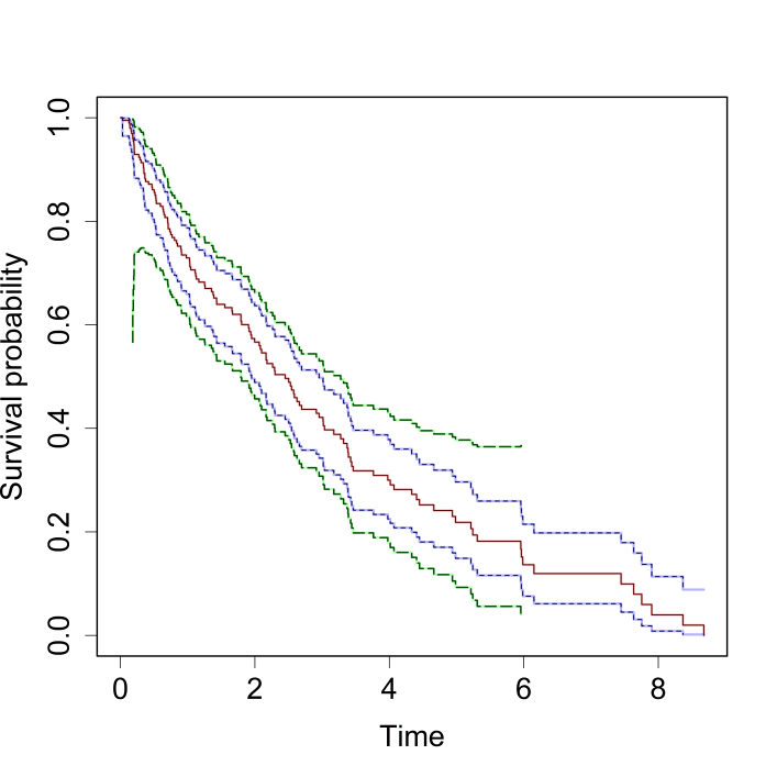
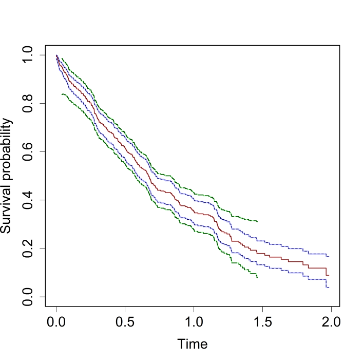
Figure 1 displays the KM estimators, pointwise 95% confidence intervals and simultaneous 95% confidence bands computed by the proposed method and existing maximum likelihood approach under one sample from Examples 1 and 2. It can be seen that although with different target functions, the KM estimator by the proposed method is the same as the traditional one. The 95% confidence intervals are exactly the same as that by Greenwood’s formula. In addition, the 95% confidence band coincides with the one proposed by Hall and Wellner, (1980).

Tables 1 and 2 show the coverage probability and the average length of the 95% confidence interval at several time points over 100 repetitions for Examples 1 and 2. We choose seven time points $1,2,\ldots,7$ in Example 1 and eight time points $0.1,0.3,\ldots,1.5$ in Example 2. Given that the KM estimator obtained by the proposed method equals the one computed via the maximum likelihood approach, the results of M-KM is the same as the existing one. The coverage probability of the 95% confidence interval in Example 1 is around 0.95 at all seven time points. However, in Example 2, the coverage probability is less than 0.95 for larger time points. We also compute the coverage probability for the confidence bands. In Example 1, the coverage probability of the confidence band is 0.97, while the value is 0.94 in Example 2. This means that the properties of the KM estimator can be successively recovered with the M-estimation theory, implying that KM estimator can be interpreted as an M-estimator.

Figure 1: KM curves (red), 95% confidence interval (blue) and 95% confidence band (green) of Examples 1 (left) and 2 (right).

Table 1: The coverage probability and the average length of the 95% confidence interval at different time points over 100 replications under Example 1.

		Time points
		1	2	3	4	5	6	7
Coverage Probability	M-KM	0.98	0.96	0.97	0.96	0.97	0.95	0.97
	KM	0.98	0.96	0.97	0.96	0.97	0.95	0.97
Length	M-KM	0.1299	0.1516	0.1541	0.149	0.1401	0.1298	0.1196
	KM	0.1299	0.1516	0.1541	0.149	0.1401	0.1298	0.1196

Table 2: The coverage probability and the average length of the 95% confidence interval at different time points over 100 replications under Example 2.

		Time points
		0.1	0.3	0.5	0.7	0.9	1.1	1.3	1.5
Coverage Probability	M-KM	0.94	0.92	0.88	0.88	0.85	0.89	0.91	0.84
	KM	0.94	0.92	0.88	0.88	0.85	0.89	0.91	0.84
Length	M-KM	0.052	0.079	0.0906	0.0962	0.0989	0.1005	0.1026	0.1078
	KM	0.052	0.079	0.0905	0.0962	0.0989	0.1005	0.1026	0.1078

4.2 Real Data Application

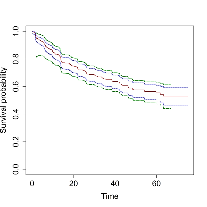
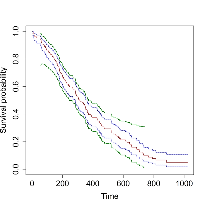
We apply the proposed method to two datasets to evaluate its performance. The first dataset is from a diabetic study, including $n=394$ observations and 8 variables. Among all observations, 197 patients are labeled “high-risk” diabetic retinopathy according to the diabetic retinopathy study (DRS). For each patient, one eye was randomly chosen to receive the laser treatment and the other one received no treatment. The event of interest is that the visual acuity dropped below 5/200. Some records were censored due to death, dropout, or the end of the study. The second dataset is from a lung cancer study involving the North Central Cancer Treatment Group of 228 patients of advance lung cancer. The survival time was measured from initiation of the study to the time when the patient died or was censored.

The KM curves and the corresponding 95% confidence intervals and 95% confidence band computed by the proposed method and existing maximum likelihood approach for both datasets are shown in Figure 2. Again, the estimation and inference result of the proposed method are the same as the existing ones, suggesting that the proposed method provides a new interpretation of the KM estimator as an M-estimator.

Figure 2: The KM curves (red), 95% confidence interval (blue) and 95% confidence band (green) for the diabetic (left) and lung cancer datasets (right).

5 Conclusions

We reconstruct the KM estimator of the survival function as a special case of an M-estimator, which can be obtained recursively via the EM algorithm. The theoretical properties of the novel estimator, including the large-sample variance and the limiting distribution, are re-established in the spirit of M-estimation theory. Simulations and real application show that the reconstructed M-estimator is equivalent to the KM estimator under the quadratic M-function and both the consequent confidence interval and confidence band coincide with those obtained under Greenwood’s formula.

Although we develop an M-estimator of the survival function, we only consider the quadratic M-function whose maximizer coincides with the KM estimator. It would be possible to develop other M-estimators of the survival function under different M-functions, such as the $L_{\rho}$-norm. In addition, since the proposed M-estimator is a nonparametric estimator for the survival function, it is possible to develop its parametric counterpart, which may not be the same as the parametric maximum likelihood estimation. It is also interesting to investigate how such nonparametric M-estimator can be utilized in fitting existing survival models with exogenous features, such as the Cox proportional hazard model.

Appendix A Proof of Theorem 1

By the definition of $E[M_{n}({\hat{S}^{(g)}})|\hat{S}^{(g)}]$, we can deduce that

$$n\big{(}E[M_{n}(S)|\hat{S}^{(g)}]-\widetilde{M}_{n}({S})\big{)}$$

$$= \sum_{\Delta_{i}=0}\int_{0}^{\infty}\big{[}-\frac{\hat{S}^{(g)}(\max\{x,X_{i}\})}{\hat{S}^{(g)}(X_{i})}+2S(x)\frac{\hat{S}^{(g)}(\max\{x,X_{i}\})}{\hat{S}^{(g)}(X_{i})}-S(x)^{2}\big{]}d\mu(x)$$

$$-\int_{0}^{X_{i}}(-1+2S(x)-S(x)^{2})d\mu(x)$$

$$= \sum_{\Delta_{i}=0}\int_{X_{i}}^{\infty}\big{[}-\frac{\hat{S}^{(g)}(x)}{\hat{S}^{(g)}(X_{i})}+2S(x)\frac{\hat{S}^{(g)}(x)}{\hat{S}^{(g)}(X_{i})}-S(x)^{2}\big{]}d\mu(x)$$

$$= \sum_{\Delta_{i}=0}\int_{X_{i}}^{\infty}-\big{[}S(x)-\frac{\hat{S}^{(g)}(x)}{\hat{S}^{(g)}(X_{i})}\big{]}^{2}d\mu(x)+\sum_{\Delta_{i}=0}\int_{X_{i}}^{\infty}\frac{\hat{S}^{(g)}(x)^{2}}{\hat{S}^{(g)}(X_{i})^{2}}d\mu(x)-\sum_{\Delta_{i}=0}\int_{X_{i}}^{\infty}\frac{\hat{S}^{(g)}(x)}{\hat{S}^{(g)}(X_{i})}d\mu(x).$$

Note that $n\big{(}E[M_{n}(S)|\hat{S}^{(g)}]-\widetilde{M}_{n}({S})\big{)}$ consists of three terms. The latter two terms are irrelevant to $S(x)$. By the Cauchy–Schwarz inequality, the former one is maximized if and only if $S(x)=\hat{S}^{(g)}(x)$.

Appendix B Proof of Theorem 2

Define $n_{(k)}=\#\{i:X_{i}=X_{(k)}\}$ and $\Delta_{(k)}=\#\{i:X_{i}=X_{(k)};\Delta_{i}=1\}$, we have that for $g=1,2,\ldots$,

$$E[M_{n}(S)|\hat{S}^{(g-1)}]$$

$$= \frac{1}{n}\sum_{k=1}^{K}\int_{0}^{\infty}\Delta_{(k)}\big{[}-I\{X_{(k)}>x\}^{2}+2S(x)I\{X_{(k)}>x\}-S(x)^{2}\big{]}d\mu(x)$$

$$+\frac{1}{n}\sum_{k=1}^{K}\int_{0}^{\infty}(n_{(k)}-\Delta_{(k)})\Big{[}-\frac{\hat{S}^{(g-1)}(\max\{x,X_{(k)}\})}{\hat{S}^{(g-1)}(X_{(k)})}+2S(x)\frac{\hat{S}^{(g-1)}(\max\{x,X_{(k)}\})}{\hat{S}^{(g-1)}(X_{(k)})}-S(x)^{2}\Big{]}d\mu(x).$$

Hence,

$$\hat{S}^{(g)}(x)= \arg\max_{S(x)\in\mathcal{S}}E[M_{n}(S)|\hat{S}^{(g-1)}]$$

$$= \frac{1}{n}\sum_{k=1}^{K}\big{[}\Delta_{(k)}I\{X_{(k)}>x\}+(n_{(k)}-\Delta_{(k)})\frac{\hat{S}^{(g-1)}(\max\{x,X_{(k)}\})}{\hat{S}^{(g-1)}(X_{(k)})}\big{]}.$$

If $\hat{S}^{(g-1)}$ is a non-increasing right-continuous function with $\hat{S}^{(g-1)}(0)=1$, it is clear that $I\{X_{(k)}>x\}$ and $\hat{S}^{(g-1)}(\max\{x,X_{(k)}\})/\hat{S}^{(g-1)}(X_{(k)})$ are both non-increasing right-continuous functions and thus $\hat{S}^{(g)}$ is a non-increasing right-continuous function with $\hat{S}^{(g)}(0)=1$. Given $\hat{S}^{(0)}$ is a non-increasing right-continuous function with $\hat{S}^{(0)}(0)=1$, by induction, we have $\hat{S}(x)$ is a non-increasing right-continuous function with $\hat{S}(0)=1$.

• For all $x\in[0,X_{(1)})$, it is obvious that $\hat{S}^{(g)}(x)=1$ for $g=0,1,\ldots$ and equation (6) holds.

• We then prove that equation (6) holds at $x=X_{(1)},\ldots,X_{(K)}$.

  • It is clear that for $g=0,1,\ldots$,

    $$\hat{S}^{(g)}(X_{(1)}) =\frac{1}{n}\big{[}\sum_{k=1}^{K}(n_{(k)}-\Delta_{(k)})+\sum_{k=2}^{K}\Delta_{(k)}\big{]}$$

    $$=1-\frac{\Delta_{(1)}}{\sum_{k=1}^{K}n_{(k)}}$$

    $$=1-\frac{\#\{i:X_{i}=X_{(1)};\Delta_{i}=1\}}{\#\{i:X_{i}\geq X_{(1)}\}}$$

    and equation (6) holds at $x=X_{(1)}$.

  • Suppose that equation (6) holds at $x=X_{(l-1)}$ ($l=2,\ldots,K$). If $\hat{S}(X_{(l-1)})=0$, $\hat{S}(X_{(l)})=0$ and thus equation (6) holds at $x=X_{(l)}$. If $\hat{S}(X_{(l-1)})\neq 0$, by the convergence condition of the EM algorithm,

    $$\hat{S}(x)= \arg\max_{S(x)\in\mathcal{S}}E[M_{n}(S)|\hat{S}]$$ (8)

    $$= \frac{1}{n}\sum_{k=1}^{K}\big{[}\Delta_{(k)}I\{X_{(k)}>x\}+(n_{(k)}-\Delta_{(k)})\frac{\hat{S}(\max\{x,X_{(k)}\})}{\hat{S}(X_{(k)})}\big{]},$$

    we have

    $$\frac{\hat{S}(X_{(l)})}{\hat{S}(X_{(l-1)})}= \frac{n_{(l)}-\Delta_{(l)}+\sum_{k=l+1}^{K}n_{(k)}+\hat{S}(X_{(l)})\sum_{k=1}^{l-1}{(n_{(k)}-\Delta_{(k)})}/{\hat{S}(X_{(k)})}}{\sum_{k=l}^{K}n_{(k)}+\hat{S}(X_{(l-1)})\sum_{k=1}^{l-1}{(n_{(k)}-\Delta_{(k)})}/{\hat{S}(X_{(k)})}}.$$

    It is clear that

    $$\frac{\hat{S}(X_{(l)})}{\hat{S}(X_{(l-1)})} =\frac{n_{(l)}-\Delta_{(l)}+\sum_{k=l+1}^{K}n_{(k)}}{\sum_{k=l}^{K}n_{(k)}}$$

    $$=1-\frac{\Delta_{(l)}}{\sum_{k=l}^{K}n_{(k)}}$$

    $$=1-\frac{\#\{i:X_{i}=X_{(l)};\Delta_{i}=1\}}{\#\{i:X_{i}\geq X_{(l)}\}}$$

    and equation (6) holds at $x=X_{(l)}$.

• Finally, we prove that equation (6) holds for $x\in(X_{(l-1)},X_{(l)})$ ($l=2,\ldots,K$) and for $x\in(X_{(K)},\infty)$.

  • For $x\in(X_{(l-1)},X_{(l)})$ ($l=2,\ldots,K$), if $\hat{S}(X_{(l-1)})=0$, $\hat{S}(x)=0$ and thus equation (6) holds; otherwise, by the convergence condition (8) of the EM algorithm, we have

    $$\frac{\hat{S}(x)}{\hat{S}(X_{(l-1)})}= \frac{n_{(l)}-\Delta_{(l)}+\sum_{k=l+1}^{K}n_{(k)}+\hat{S}(x)\sum_{k=1}^{l-1}{(n_{(k)}-\Delta_{(k)})}/{\hat{S}(X_{(k)})}}{\sum_{k=l}^{K}n_{(k)}+\hat{S}(X_{(l-1)})\sum_{k=1}^{l-1}{(n_{(k)}-\Delta_{(k)})}/{\hat{S}(X_{(k)})}},$$

    implying that $\hat{S}(x)/\hat{S}(X_{(l-1)})=1$. Thus, equation (6) holds.

  • For $x\in(X_{(K)},\infty)$, if $\hat{S}(X_{(K)})=0$, $\hat{S}(x)=0$ and thus equation (6) holds; otherwise, it is clear that for $g=1,2,\ldots$,

    $$\frac{\hat{S}^{(g)}(x)}{\hat{S}^{(g)}(X_{(K)})}= \frac{\sum_{k=1}^{K}(n_{(k)}-\Delta_{(k)})\hat{S}^{(g-1)}(x)}{\sum_{k=1}^{K}(n_{(k)}-\Delta_{(k)})\hat{S}^{(g-1)}(X_{(K)})}$$

    $$= \frac{\hat{S}^{(g-1)}(x)}{\hat{S}^{(g-1)}(X_{(K)})}$$

    $$= \cdots$$

    $$= \frac{\hat{S}^{(0)}(x)}{\hat{S}^{(0)}(X_{(K)})}$$

    $$= 1.$$

    Therefore,

    $$\frac{\hat{S}(x)}{\hat{S}(X_{(K)})}=\lim\limits_{g\to\infty}\frac{\hat{S}^{(g)}(x)}{\hat{S}^{(g)}(X_{(K)})}=1,$$

    and equation (6) holds.

References

• Altman and Bland, (1998) Altman, D. G. and Bland, J. M. (1998). Time to event (survival) data. British Medical Journal, 317(7156):468–469.
• Breslow and Crowley, (1974) Breslow, N. and Crowley, J. (1974). A large sample study of the life table and product limit estimates under random censorship. The Annals of Statistics, 2(3):437–453.
• Cox, (1972) Cox, D. R. (1972). Regression models and life-tables. Journal of the Royal Statistical Society. Series B (Methodological), 34(2):187–220.
• Danacica and Babucea, (2010) Danacica, D.-E. and Babucea, A.-G. (2010). Using survival analysis in economics. Survival, 11:15.
• Greenwood, (1926) Greenwood, M. (1926). A report on the natural duration of cancer. A Report on the Natural Duration of Cancer., (33).
• Hall and Wellner, (1980) Hall, W. J. and Wellner, J. A. (1980). Confidence bands for a survival curve from censored data. Biometrika, 67(1):133–143.
• Huh et al., (2011) Huh, W. T., Levi, R., Rusmevichientong, P., and Orlin, J. B. (2011). Adaptive data-driven inventory control with censored demand based on kaplan-meier estimator. Operations Research, 59(4):929–941.
• Johansen, (1978) Johansen, S. (1978). The product limit estimator as maximum likelihood estimator. Scandinavian Journal of Statistics, pages 195–199.
• Kaminski and Geisler, (2012) Kaminski, D. and Geisler, C. (2012). Survival analysis of faculty retention in science and engineering by gender. Science, 335(6070):864–866.
• Kaplan and Meier, (1958) Kaplan, E. L. and Meier, P. (1958). Nonparametric estimation from incomplete observations. Journal of the American statistical association, 53(282):457–481.
• Mantel, (1966) Mantel, N. (1966). Evaluation of survival data and two new rank order statistics arising in its consideration. Cancer chemotherapy reports, 50(3):163—170.
• Peterson Jr, (1977) Peterson Jr, A. V. (1977). Expressing the kaplan-meier estimator as a function of empirical subsurvival functions. Journal of the American Statistical Association, 72(360a):854–858.
• Susarla and Ryzin, (1976) Susarla, V. and Ryzin, J. V. (1976). Nonparametric bayesian estimation of survival curves from incomplete observations. Journal of the American Statistical Association, 71(356):897–902.