Optimizing Approximate Leave-one-out Cross-validation to Tune Hyperparameters

Abstract

For a large class of regularized models, leave-one-out cross-validation can be efficiently estimated with an approximate leave-one-out formula (ALO). We consider the problem of adjusting hyperparameters so as to optimize ALO. We derive efficient formulas to compute the gradient and hessian of ALO and show how to apply a second-order optimizer to find hyperparameters. We demonstrate the usefulness of the proposed approach by finding hyperparameters for regularized logistic regression and ridge regression on various real-world data sets.

Keywords: hyperparameter optimization, regularization, logistic regression, ridge regression, trust-region methods

1 Introduction

Let ${\cal D}=\{\left(y_{1},\boldsymbol{x}_{1}\right),\cdots,\left(y_{n},\boldsymbol{x}_{n}\right)\}$ denote a data set, where $\boldsymbol{x}_{i}\in\mathbb{R}^{p}$ are features and $y_{i}\in\mathbb{R}$ are responses. In many applications, we model the observations as independent and identically distributed draws from an unknown joint distribution of the form $q\left(y_{i},\boldsymbol{x}_{i}\right)=q_{1}\left(y_{i}\mid\boldsymbol{x}_{i}^{\top}\boldsymbol{\beta}_{*}\right)q_{2}\left(\boldsymbol{\beta}_{*}\right)$, and we estimate $\boldsymbol{\beta}_{*}$ using the optimization problem

$$\boldsymbol{\hat{\beta}}\triangleq\operatorname*{argmin}_{\boldsymbol{\beta}}\left\{\sum_{i=1}^{n}\ell\left(y_{i}\mid\boldsymbol{x}_{i}^{\top}\boldsymbol{\beta}\right)+R_{\boldsymbol{\lambda}}\left(\boldsymbol{\beta}\right)\right\},$$ (1)

where $\ell$ is a loss function, $R_{\boldsymbol{\lambda}}(\boldsymbol{\beta})=\sum_{j=1}^{p}r_{j,\boldsymbol{\lambda}}(\hat{\beta}_{j})$ is a regularizer, and $\boldsymbol{\lambda}$ represents hyperparameters. $R_{\boldsymbol{\lambda}}$ controls the complexity of the model by penalizing larger values of $\boldsymbol{\beta}$ and can prevent overfitting. We aim to select $\boldsymbol{\lambda}$ so as to minimize the out-of-sample prediction error

$$\mathrm{Err}_{\mathrm{out}}\triangleq\mathbb{E}\left[\ell\left(y_{o}\mid\boldsymbol{x}_{o}^{\top}\boldsymbol{\hat{\beta}}\right)\mid{\cal D}\right],$$

where $\left(y_{o},\boldsymbol{x}_{o}\right)$ is an unseen sample from the distribution $q\left(y,\boldsymbol{x}\right)$. Because $q$ is unknown, we estimate $\mathrm{Err}_{\mathrm{out}}$ with a function $f\left(\boldsymbol{\lambda}\mid{\cal D}\right)$ and apply a hyperparameter optimization algorithm to find

$$\boldsymbol{\hat{\lambda}}\triangleq\operatorname*{argmin}_{\boldsymbol{\lambda}}f\left(\boldsymbol{\lambda}\mid{\cal D}\right).$$

Empirical evidence has shown leave-one-out cross-validation (LO) to be an accurate method for estimating $\mathrm{Err}_{\mathrm{out}}$ (Rad et al., 2020). In general, LO can be expensive to compute, requiring a model to be fit $n$ times; however, under certain conditions, it can be efficiently estimated using a closed-form approximate leave-one-out formula (ALO), and the approximation has been shown to be accurate in high-dimensional settings (Rad and Maleki, 2020). In addition, for the special case of ridge regression, ALO is exact and equivalent to Allen’s PRESS (Allen, 1974).

In this paper, we derive efficient formulas to compute the gradient and hessian of ALO, given a smooth loss function and a smooth regularizer, and we show how to apply a trust-region algorithm to find hyperparameters for several different classes of regularized models.

1.1 Relevant Work

Grid search is a commonly used approach for hyperparameter optimization. Although it can work well for models with only a single hyperparameter, it requires a search space to be specified and quickly becomes inefficient when multiple hyperparameters are used (Bergstra and Bengio, 2012). Other scalable gradient-based approaches have focused on using holdout sets to approximate $\mathrm{Err}_{\mathrm{out}}$ (Do et al., 2008; Bengio, 2000). Using ALO, we expect our objective function to be a more accurate proxy for $\mathrm{Err}_{\mathrm{out}}$. We further improve on previous approaches by computing the hessian of our objective function and applying a trust-region algorithm, allowing us to make global convergence guarantees.

1.2 Notation

We denote vectors by lowercase bold letters and matrices by uppercase bold letters. We use the notation $\mathrm{vec}\left[\left\{a_{i}\right\}_{i}\right]$ to denote the column vector $\left(a_{1},a_{2},\ldots\right)^{\top}$. For a function $f\colon\mathbb{R}\to\mathbb{R}$, we denote its 1^st, 2^nd, 3^rd, and 4^th derivatives by $\dot{f}$, $\ddot{f}$, $\dddot{f}$, and $\ddddot{f}$, respectively. Finally, given a function $f\colon\mathbb{R}^{p}\to\mathbb{R}$, we denote the gradient by $\nabla f$ and the hessian by $\nabla^{2}f$.

2 Preliminary: Trust-region Methods

Let $f\colon\mathbb{R}^{p}\to\mathbb{R}$ denote a twice-differentiable objective function. Trust-region methods are iterative, second-order optimization algorithms that produce a sequence $\left\{\boldsymbol{x}_{k}\right\}$, where the $k$^th iteration is generated by updating the previous iteration with a solution to the subproblem (Sorensen, 1982)

$$\boldsymbol{x}_{k} =\boldsymbol{x}_{k-1}+\boldsymbol{\hat{s}}_{k}\quad\mbox{and}$$

$$\boldsymbol{\hat{s}}_{k} =\operatorname*{argmin}_{\boldsymbol{s}}\left\{f\left(\boldsymbol{x}_{k-1}\right)+\nabla f\left(\boldsymbol{x}_{k-1}\right)^{\top}\boldsymbol{s}+\frac{1}{2}\boldsymbol{s}^{\top}\nabla^{2}f\left(\boldsymbol{x}_{k-1}\right)\boldsymbol{s}\right\}$$

$$\phantom{=}\quad\mathrm{s.t.}\quad\|\boldsymbol{s}\|\leq\delta_{k}.$$

The subproblem minimizes the second-order approximation of $f$ at $\boldsymbol{x}_{k-1}$ within the neighborhood $\|\boldsymbol{s}\|\leq\delta_{k}$, called the trust region. Using the trust region, we can restrict the second-order approximation to areas where it models $f$ well. Efficient algorithms exist to solve the subproblem regardless of whether $\nabla^{2}f(\boldsymbol{x}_{k-1})$ is positive-definite, making trust-region methods well-suited for non-convex optimization problems (Moré and Sorensen, 1983). With proper rules for updating $\delta_{k}$ and standard assumptions, such as Lipschitz continuity of $\nabla f$, trust-region methods are globally convergent. Moreover, if $\nabla^{2}f$ is Lipschitz continuous for all $\boldsymbol{x}$ sufficiently close to a nondegenerate second-order stationary point $\boldsymbol{x}_{*}$, where $\nabla^{2}f(\boldsymbol{x}_{*})$ is positive-definite, then trust-region methods have quadratic local convergence (Nocedal and Wright, 1999).

3 Preliminary: ALO

Put $\ell_{i}(u)\triangleq\ell(y_{i}\mid u)$. The LO estimate for $\mathrm{Err}_{\mathrm{out}}$ is defined as

$$\mathrm{LO}_{\boldsymbol{\lambda}}\triangleq\frac{1}{n}\sum_{i=1}^{n}\ell_{i}\left(\boldsymbol{x}_{i}^{\top}\boldsymbol{\hat{\beta}}_{/i}\right),$$

where

$$\boldsymbol{\hat{\beta}}_{/i}\triangleq\operatorname*{argmin}_{\boldsymbol{\beta}}\left\{\sum_{j\neq i}\ell_{j}\left(\boldsymbol{x}_{j}^{\top}\boldsymbol{\beta}\right)+R_{\boldsymbol{\lambda}}\left(\boldsymbol{\beta}\right)\right\}.$$ (2)

ALO works by finding $\boldsymbol{\hat{\beta}}$ and then using a single step of Newton’s method to approximate $\boldsymbol{\hat{\beta}}_{/i}$ from the gradient and hessian of Equation 2 at $\boldsymbol{\hat{\beta}}$. Let $\boldsymbol{g}_{/i}$ and $\boldsymbol{H}_{/i}$ denote the gradient and hessian, respectively, of Equation 2 at $\boldsymbol{\hat{\beta}}$. The ALO approximation to $\boldsymbol{\hat{\beta}}_{/i}$ is $\boldsymbol{\tilde{\beta}}_{/i}\triangleq\boldsymbol{\hat{\beta}}-\boldsymbol{H}_{/i}^{-1}\boldsymbol{g}_{/i}$, and

$$\mathrm{ALO}_{\boldsymbol{\lambda}}\triangleq\frac{1}{n}\sum_{i=1}^{n}\ell_{i}\left(\boldsymbol{x}_{i}^{\top}\boldsymbol{\tilde{\beta}}_{/i}\right).$$

Computed naively, this formula would require solving a linear system of order $p$ $n$ times, but we can achieve a more efficient form by applying the matrix inversion lemma. Let $\boldsymbol{X}$ represent the feature matrix whose i^th row is $\boldsymbol{x}_{i}$; let $\boldsymbol{H}$ denote the hessian of Equation 1 at $\boldsymbol{\hat{\beta}}$. Define $\boldsymbol{W}\triangleq\nabla^{2}R_{\boldsymbol{\lambda}}(\boldsymbol{\hat{\beta}})$ and $u_{i}=\boldsymbol{x}_{i}\boldsymbol{\hat{\beta}}$. Then,

$$\boldsymbol{H}=\boldsymbol{X}^{\top}\boldsymbol{A}\boldsymbol{X}+\boldsymbol{W},$$

where $\boldsymbol{A}$ is a diagonal matrix with $\boldsymbol{A}_{ii}=\ddot{\ell_{i}}\left(u_{i}\right)$, and

$$\mathrm{ALO}_{\boldsymbol{\lambda}}=\frac{1}{n}\sum_{i=1}^{n}\ell_{i}\left(u_{i}+\frac{\dot{\ell}_{i}\left(u_{i}\right)h_{i}}{1-\ddot{\ell}_{i}\left(u_{i}\right)h_{i}}\right),$$

where $h_{i}\triangleq\boldsymbol{x}_{i}^{\top}\boldsymbol{H}^{-1}\boldsymbol{x}_{i}$. See Rad and Maleki (2020) for a derivation.

4 Optimizing ALO

Put

$$\tilde{u}_{/i}\triangleq u_{i}+\frac{\dot{\ell}_{i}\left(u_{i}\right)h_{i}}{1-\ddot{\ell}_{i}\left(u_{i}\right)h_{i}}\quad\mbox{and}\quad f\left(\boldsymbol{\lambda}\right)\triangleq\frac{1}{n}\sum_{i=1}^{n}\ell_{i}(\tilde{u}_{/i}).$$

We present formulas for computing $\nabla f$ and $\nabla^{2}f$. See Appendix A and Appendix B for derivations. In general, $\nabla^{2}f$ will not be positive-definite; however, we can use a trust-region algorithm to find local minimums.

Theorem 1

The gradient of $\mathrm{ALO}_{\boldsymbol{\lambda}}$ can be computed as

$$\frac{\partial f}{\partial\lambda_{s}} =\frac{1}{n}\sum_{i=1}^{n}\left(\dot{\ell}_{i}(\tilde{u}_{/i})\times\frac{\partial\tilde{u}_{/i}}{\partial\lambda_{s}}\right),$$

where

$$\frac{\partial\tilde{u}_{/i}}{\partial\lambda_{s}} =\frac{\partial\tilde{u}_{/i}}{\partial u_{i}}\times\frac{\partial u_{i}}{\partial\lambda_{s}}+\frac{\partial\tilde{u}_{/i}}{\partial h_{i}}\times\frac{\partial h_{i}}{\partial\lambda_{s}},$$

$$\frac{\partial u_{i}}{\partial\lambda_{s}} =\boldsymbol{x}_{i}^{\top}\frac{\partial\boldsymbol{\hat{\beta}}}{\partial\lambda_{s}},$$

$$\frac{\partial\boldsymbol{\hat{\beta}}}{\partial\lambda_{s}} =-\boldsymbol{H}^{-1}\frac{\partial\nabla R_{\boldsymbol{\lambda}}}{\partial\lambda_{s}}(\boldsymbol{\hat{\beta}}),$$

$$\frac{\partial h_{i}}{\partial\lambda_{s}} =-\boldsymbol{x}_{i}^{\top}\boldsymbol{H}^{-1}\frac{\partial\boldsymbol{H}}{\partial\lambda_{s}}\boldsymbol{H}^{-1}\boldsymbol{x}_{i},\mbox{ and }$$

$$\frac{\partial\boldsymbol{H}}{\partial\lambda_{s}} =\boldsymbol{X}^{\top}\frac{\partial\boldsymbol{A}}{\partial\lambda_{s}}\boldsymbol{X}+\frac{\partial\boldsymbol{W}}{\partial\lambda_{s}}.$$

The diagonal matrices $\boldsymbol{A}$ and $\boldsymbol{W}$ have derivatives

$$\left(\frac{\partial\boldsymbol{A}}{\partial\lambda_{s}}\right)_{ii} =\dddot{\ell}_{i}\left(u_{i}\right)\times\frac{\partial u_{i}}{\partial\lambda_{s}}\quad\mbox{and}$$

$$\left(\frac{\partial\boldsymbol{W}}{\partial\lambda_{s}}\right)_{jj} =\frac{\partial\ddot{r}_{j,\boldsymbol{\lambda}}}{\partial\lambda_{s}}(\hat{\beta}_{j})+\dddot{r}_{j,\boldsymbol{\lambda}}(\hat{\beta}_{j})\times\frac{\partial\hat{\beta}_{j}}{\partial\lambda_{s}},$$

and $\tilde{u}_{/i}$ has derivatives

$$\frac{\partial\tilde{u}_{/i}}{\partial u_{i}} =\frac{1}{1-\ddot{\ell}_{i}\left(u_{i}\right)h_{i}}+\frac{\dot{\ell}_{i}\left(u_{i}\right)\dddot{\ell}_{i}\left(u_{i}\right)h_{i}^{2}}{(1-\ddot{\ell}_{i}\left(u_{i}\right)h_{i})^{2}}\quad\mbox{and}$$

$$\frac{\partial\tilde{u}_{/i}}{\partial h_{i}} =\frac{\dot{\ell}_{i}\left(u_{i}\right)}{(1-\ddot{\ell}_{i}\left(u_{i}\right)h_{i})^{2}}.$$

Theorem 2

The hessian of $\mathrm{ALO}_{\boldsymbol{\lambda}}$ can be computed as

$$\frac{\partial^{2}f}{\partial\lambda_{s}\partial\lambda_{t}} =\frac{1}{n}\sum_{i=1}^{n}\left(\ddot{\ell}_{i}(\tilde{u}_{/i})\times\frac{\partial\tilde{u}_{/i}}{\partial\lambda_{s}}\times\frac{\partial\tilde{u}_{/i}}{\partial\lambda_{t}}+\dot{\ell}_{i}(\tilde{u}_{/i})\times\frac{\partial^{2}\tilde{u}_{/i}}{\partial\lambda_{s}\partial\lambda_{t}}\right),$$

where

$$\frac{\partial^{2}\tilde{u}_{/i}}{\partial\lambda_{s}\partial\lambda_{t}} =\!\begin{multlined}\frac{\partial\tilde{u}_{/i}}{\partial u_{i}}\times\frac{\partial^{2}u_{i}}{\partial\lambda_{s}\partial\lambda_{t}}+\frac{\partial^{2}\tilde{u}_{/i}}{\partial u_{i}^{2}}\times\frac{\partial u_{i}}{\partial\lambda_{s}}\times\frac{\partial u_{i}}{\partial\lambda_{t}}\\ +\frac{\partial^{2}\tilde{u}_{/i}}{\partial u_{i}\partial h_{i}}\times\left[\frac{\partial u_{i}}{\partial\lambda_{s}}\times\frac{\partial h_{i}}{\partial\lambda_{t}}+\frac{\partial u_{i}}{\partial\lambda_{t}}\times\frac{\partial h_{i}}{\partial\lambda_{s}}\right]\\ +\frac{\partial\tilde{u}_{/i}}{\partial h_{i}}\times\frac{\partial^{2}h_{i}}{\partial\lambda_{s}\partial\lambda_{t}}+\frac{\partial^{2}\tilde{u}_{/i}}{\partial h_{i}^{2}}\times\frac{\partial h_{i}}{\partial\lambda_{s}}\times\frac{\partial h_{i}}{\partial\lambda_{t}},\end{multlined}\frac{\partial\tilde{u}_{/i}}{\partial u_{i}}\times\frac{\partial^{2}u_{i}}{\partial\lambda_{s}\partial\lambda_{t}}+\frac{\partial^{2}\tilde{u}_{/i}}{\partial u_{i}^{2}}\times\frac{\partial u_{i}}{\partial\lambda_{s}}\times\frac{\partial u_{i}}{\partial\lambda_{t}}\\ +\frac{\partial^{2}\tilde{u}_{/i}}{\partial u_{i}\partial h_{i}}\times\left[\frac{\partial u_{i}}{\partial\lambda_{s}}\times\frac{\partial h_{i}}{\partial\lambda_{t}}+\frac{\partial u_{i}}{\partial\lambda_{t}}\times\frac{\partial h_{i}}{\partial\lambda_{s}}\right]\\ +\frac{\partial\tilde{u}_{/i}}{\partial h_{i}}\times\frac{\partial^{2}h_{i}}{\partial\lambda_{s}\partial\lambda_{t}}+\frac{\partial^{2}\tilde{u}_{/i}}{\partial h_{i}^{2}}\times\frac{\partial h_{i}}{\partial\lambda_{s}}\times\frac{\partial h_{i}}{\partial\lambda_{t}},$$

$$\frac{\partial^{2}u_{i}}{\partial\lambda_{s}\partial\lambda_{t}} =\boldsymbol{x}_{i}^{\top}\frac{\partial^{2}\boldsymbol{\hat{\beta}}}{\partial\lambda_{s}\partial\lambda_{t}},$$

$$\frac{\partial^{2}\boldsymbol{\hat{\beta}}}{\partial\lambda_{s}\partial\lambda_{t}} =\!\begin{multlined}-\boldsymbol{H}^{-1}\boldsymbol{X}^{\top}\cdot\mathrm{vec}\left[\left\{\dddot{\ell}_{i}\left(u_{i}\right)\times\frac{\partial u_{i}}{\partial\lambda_{s}}\times\frac{\partial u_{i}}{\partial\lambda_{t}}\right\}_{i}\right]\\ -\boldsymbol{H}^{-1}\frac{\partial\nabla^{2}R_{\boldsymbol{\lambda}}}{\partial\lambda_{s}}(\boldsymbol{\hat{\beta}})\frac{\partial\boldsymbol{\hat{\beta}}}{\partial\lambda_{t}}-\boldsymbol{H}^{-1}\frac{\partial\nabla^{2}R_{\boldsymbol{\lambda}}}{\partial\lambda_{t}}(\boldsymbol{\hat{\beta}})\frac{\partial\boldsymbol{\hat{\beta}}}{\partial\lambda_{s}}-\boldsymbol{H}^{-1}\frac{\partial\nabla R_{\boldsymbol{\lambda}}}{\partial\lambda_{s}\partial\lambda_{t}}(\boldsymbol{\hat{\beta}})\\ -\boldsymbol{H}^{-1}\cdot\mathrm{vec}\left[\left\{\dddot{r}_{j,\boldsymbol{\lambda}}(\hat{\beta}_{j})\times\frac{\partial\hat{\beta}_{j}}{\partial\lambda_{s}}\times\frac{\partial\hat{\beta}_{j}}{\partial\lambda_{t}}\right\}_{j}\right],\end{multlined}-\boldsymbol{H}^{-1}\boldsymbol{X}^{\top}\cdot\mathrm{vec}\left[\left\{\dddot{\ell}_{i}\left(u_{i}\right)\times\frac{\partial u_{i}}{\partial\lambda_{s}}\times\frac{\partial u_{i}}{\partial\lambda_{t}}\right\}_{i}\right]\\ -\boldsymbol{H}^{-1}\frac{\partial\nabla^{2}R_{\boldsymbol{\lambda}}}{\partial\lambda_{s}}(\boldsymbol{\hat{\beta}})\frac{\partial\boldsymbol{\hat{\beta}}}{\partial\lambda_{t}}-\boldsymbol{H}^{-1}\frac{\partial\nabla^{2}R_{\boldsymbol{\lambda}}}{\partial\lambda_{t}}(\boldsymbol{\hat{\beta}})\frac{\partial\boldsymbol{\hat{\beta}}}{\partial\lambda_{s}}-\boldsymbol{H}^{-1}\frac{\partial\nabla R_{\boldsymbol{\lambda}}}{\partial\lambda_{s}\partial\lambda_{t}}(\boldsymbol{\hat{\beta}})\\ -\boldsymbol{H}^{-1}\cdot\mathrm{vec}\left[\left\{\dddot{r}_{j,\boldsymbol{\lambda}}(\hat{\beta}_{j})\times\frac{\partial\hat{\beta}_{j}}{\partial\lambda_{s}}\times\frac{\partial\hat{\beta}_{j}}{\partial\lambda_{t}}\right\}_{j}\right],$$

$$\frac{\partial^{2}h_{i}}{\partial\lambda_{s}\partial\lambda_{t}} =2\boldsymbol{x}_{i}^{\top}\boldsymbol{H}^{-1}\frac{\partial\boldsymbol{H}}{\partial\lambda_{s}}\boldsymbol{H}^{-1}\frac{\partial\boldsymbol{H}}{\partial\lambda_{t}}\boldsymbol{H}^{-1}\boldsymbol{x}_{i}-\boldsymbol{x}_{i}^{\top}\boldsymbol{H}^{-1}\frac{\partial^{2}\boldsymbol{H}}{\partial\lambda_{s}\partial\lambda_{t}}\boldsymbol{H}^{-1}\boldsymbol{x}_{i},\mbox{ and}$$

$$\frac{\partial^{2}\boldsymbol{H}}{\partial\lambda_{s}\partial\lambda_{t}} =\boldsymbol{X}^{\top}\frac{\partial^{2}\boldsymbol{A}}{\partial\lambda_{s}\partial\lambda_{t}}\boldsymbol{X}+\frac{\partial^{2}\boldsymbol{W}}{\partial\lambda_{s}\partial\lambda_{t}}.$$

The diagonal matrices $\boldsymbol{A}$ and $\boldsymbol{W}$ have second derivatives

$$\left(\frac{\partial^{2}\boldsymbol{A}}{\partial\lambda_{s}\partial\lambda_{t}}\right)_{ii} =\dddot{\ell}_{i}\left(u_{i}\right)\times\frac{\partial^{2}u_{i}}{\partial\lambda_{s}\partial\lambda_{t}}+\ddddot{\ell}_{i}\left(u_{i}\right)\times\frac{\partial u_{i}}{\partial\lambda_{s}}\times\frac{\partial u_{i}}{\partial\lambda_{t}}\quad\mbox{and}$$

$$\left(\frac{\partial^{2}\boldsymbol{W}}{\partial\lambda_{s}\partial\lambda_{t}}\right)_{jj} =\!\begin{multlined}\frac{\partial^{2}\ddot{r}_{j,\boldsymbol{\lambda}}}{\partial\lambda_{s}\partial\lambda_{t}}(\hat{\beta}_{j})+\frac{\partial\dddot{r}_{j,\boldsymbol{\lambda}}}{\partial\lambda_{s}}(\hat{\beta}_{j})\times\frac{\partial\hat{\beta}_{j}}{\partial\lambda_{t}}+\frac{\partial\dddot{r}_{j,\boldsymbol{\lambda}}}{\partial\lambda_{t}}(\hat{\beta}_{j})\times\frac{\partial\hat{\beta}_{j}}{\partial\lambda_{s}}\\ +\dddot{r}_{j,\boldsymbol{\lambda}}(\hat{\beta}_{j})\times\frac{\partial^{2}\hat{\beta}_{j}}{\partial\lambda_{s}\partial\lambda_{t}}+\ddddot{r}_{j,\boldsymbol{\lambda}}(\hat{\beta}_{j})\times\frac{\partial\hat{\beta}_{j}}{\partial\lambda_{s}}\times\frac{\partial\hat{\beta}_{j}}{\partial\lambda_{t}},\end{multlined}\frac{\partial^{2}\ddot{r}_{j,\boldsymbol{\lambda}}}{\partial\lambda_{s}\partial\lambda_{t}}(\hat{\beta}_{j})+\frac{\partial\dddot{r}_{j,\boldsymbol{\lambda}}}{\partial\lambda_{s}}(\hat{\beta}_{j})\times\frac{\partial\hat{\beta}_{j}}{\partial\lambda_{t}}+\frac{\partial\dddot{r}_{j,\boldsymbol{\lambda}}}{\partial\lambda_{t}}(\hat{\beta}_{j})\times\frac{\partial\hat{\beta}_{j}}{\partial\lambda_{s}}\\ +\dddot{r}_{j,\boldsymbol{\lambda}}(\hat{\beta}_{j})\times\frac{\partial^{2}\hat{\beta}_{j}}{\partial\lambda_{s}\partial\lambda_{t}}+\ddddot{r}_{j,\boldsymbol{\lambda}}(\hat{\beta}_{j})\times\frac{\partial\hat{\beta}_{j}}{\partial\lambda_{s}}\times\frac{\partial\hat{\beta}_{j}}{\partial\lambda_{t}},$$

and $\tilde{u}_{/i}$ has second derivatives

$$\frac{\partial^{2}\tilde{u}_{/i}}{\partial u_{i}^{2}} =\frac{\dddot{\ell}_{i}\left(u_{i}\right)h_{i}}{(1-\ddot{\ell}_{i}\left(u_{i}\right)h_{i})^{2}}+\frac{(\ddot{\ell}_{i}\left(u_{i}\right)\dddot{\ell}_{i}\left(u_{i}\right)+\dot{\ell}_{i}\left(u_{i}\right)\ddddot{\ell}_{i}\left(u_{i}\right))h_{i}^{2}}{(1-\ddot{\ell}_{i}\left(u_{i}\right)h_{i})^{2}}+\frac{2\dot{\ell}_{i}\left(u_{i}\right)\dddot{\ell}_{i}\left(u_{i}\right)^{2}h_{i}^{3}}{(1-\ddot{\ell}_{i}\left(u_{i}\right)h_{i})^{3}},$$

$$\frac{\partial^{2}\tilde{u}_{/i}}{\partial u_{i}\partial h_{i}} =\frac{\ddot{\ell}_{i}\left(u_{i}\right)}{(1-\ddot{\ell}_{i}\left(u_{i}\right)h_{i})^{2}}+\frac{2\dot{\ell}_{i}\left(u_{i}\right)\dddot{\ell}_{i}\left(u_{i}\right)h_{i}}{(1-\ddot{\ell}_{i}\left(u_{i}\right)h_{i})^{3}},\mbox{ and}$$

$$\frac{\partial^{2}\tilde{u}_{/i}}{\partial h_{i}^{2}} =\frac{2\dot{\ell}_{i}\left(u_{i}\right)\ddot{\ell}_{i}\left(u_{i}\right)}{(1-\ddot{\ell}_{i}\left(u_{i}\right)h_{i})^{3}}.$$

4.1 Computational Complexity

Let $q$ denote the number of hyperparameters. How best to proceed with the computations will depend on which is greater $n$ or $p$. We assume first that $n>p$. $\boldsymbol{H}$ and its Cholesky factorization $\boldsymbol{L}$ can be computed in $\mathcal{O}\left(p^{2}n\right)$ operations. Let $\boldsymbol{h}$ denote the vector of $h_{i}$ values. The complexity of computing the ALO value, gradient, and hessian is dominated by the cost of evaluating $\boldsymbol{h}$ and its derivatives. Using the formula

$$h_{i}=\|\boldsymbol{L}^{-1}\boldsymbol{x}_{i}\|^{2},$$

$\boldsymbol{h}$ can be computed with $\mathcal{O}\left(p^{2}n\right)$ operations. For the derivatives of $\boldsymbol{h}$, we first compute the matrices $\frac{\partial\boldsymbol{H}}{\partial\lambda_{s}}$, which can be done in $\mathcal{O}\left(p^{2}qn\right)$ operations. The derivatives can then, also, be computed with $\mathcal{O}\left(p^{2}qn\right)$ operations using the formulas

$$\boldsymbol{t}_{i}={\boldsymbol{L}^{-1}}^{\top}\boldsymbol{L}^{-1}\boldsymbol{x}_{i}\quad\mbox{and}\quad\frac{\partial h_{i}}{\partial\lambda_{s}}=\boldsymbol{t}_{i}^{\top}\frac{\partial\boldsymbol{H}}{\partial\lambda_{s}}\boldsymbol{t}_{i}.$$

For the second derivatives of $\boldsymbol{h}$, we, similarly, first compute the matrices $\frac{\partial^{2}\boldsymbol{H}}{\partial\lambda_{s}\partial\lambda_{t}}$, which can be done in $\mathcal{O}\left(p^{2}q^{2}n\right)$ operations, and then compute

$$\boldsymbol{r}_{si}=\boldsymbol{L}^{-1}\frac{\partial\boldsymbol{H}}{\partial\lambda_{s}}\boldsymbol{H}^{-1}\boldsymbol{x}_{i}\quad\mbox{and}\quad\frac{\partial^{2}h_{i}}{\partial\lambda_{s}\partial\lambda_{t}}=\boldsymbol{r}_{si}^{\top}\boldsymbol{r}_{ti}-\boldsymbol{t}_{i}^{\top}\frac{\partial^{2}\boldsymbol{H}}{\partial\lambda_{s}\partial\lambda_{t}}\boldsymbol{t}_{i}$$

with $\mathcal{O}\left(p^{2}q^{2}n\right)$ operations.

When $p>n$ and $\boldsymbol{W}$ is nonsingular, we can achieve better complexity by evaluating the equations in a different order. We apply the matrix inversion lemma to $\boldsymbol{H}^{-1}=\left[\boldsymbol{X}^{\top}\boldsymbol{A}\boldsymbol{X}+\boldsymbol{W}\right]^{-1}$ to obtain

$$\boldsymbol{H}^{-1}=\boldsymbol{W}^{-1}+\boldsymbol{W}^{-1}\boldsymbol{X}^{\top}\left[\boldsymbol{A}^{-1}+\boldsymbol{X}\boldsymbol{W}^{-1}\boldsymbol{X}^{\top}\right]^{-1}\boldsymbol{X}\boldsymbol{W}^{-1}.$$

Computing the matrix $\boldsymbol{A}^{-1}+\boldsymbol{X}\boldsymbol{W}^{-1}\boldsymbol{X}^{\top}$ and its Cholesky factorization can be done in $\mathcal{O}\left(n^{2}p\right)$ operations, and a product $\boldsymbol{H}^{-1}b$ can be done in $\mathcal{O}\left(np\right)$ operations. Applying the same approach, where we avoid explicitly computing the $p$-by-$p$ matrices, we can compute the gradient and hessian in $\mathcal{O}\left(n^{2}qp\right)$ and $\mathcal{O}\left(n^{2}q^{2}p\right)$ operations, respectively. If $\boldsymbol{W}$ is singular but only has $k$ zero diagonal entries, where $k\ll p$, we can combine this approach with block matrix inversion and still achieve more efficient formulas.

5 Examples

By customizing $\ell_{i}$ and $R_{\lambda}$, we can adopt Theorem 1 and Theorem 2 to a broad range of models. Putting $\ell_{i}(u)\triangleq(y_{i}-u)^{2}$ gives us regularized least squares; putting $\ell_{i}(u)\triangleq\log\left[1+\exp(-y_{i}u)\right]$ gives us regularized logistic regression. If we define

$$R_{\lambda}(\boldsymbol{\beta})\triangleq\lambda^{2}\left\|\boldsymbol{\beta}\right\|^{2},$$

we have standard ridge regularization. Defining

$$R_{\boldsymbol{\lambda}}(\boldsymbol{\beta})\triangleq\sum_{j=1}^{p}\lambda_{g_{j}}^{2}\lvert\beta_{j}\rvert^{2}$$

allows us to use different regularization strengths for different groups of variables, and putting

$$R_{\boldsymbol{\lambda}}(\boldsymbol{\beta})\triangleq\lambda_{1}^{2}\sum_{j=1}^{p}\lvert\beta_{j}\rvert^{1+\lambda_{2}^{2}}$$

gives us bridge regularization (Fu, 1998). We present versions of Theorem 1 and Theorem 2 for the specific cases of ridge regression and logistic regression with ridge regularization.

5.1 Ridge Regression

Because Equation 1 is a quadratic for ridge regression, the Newton approximation step in ALO is exact, $\boldsymbol{\tilde{\beta}}_{/i}=\boldsymbol{\hat{\beta}}_{/i}$, and ALO and LO are equivalent. Before stating theorems for the LO gradient and hessian, we first introduce more familiar notation. Put

$$\hat{y}_{i}\triangleq u_{i},\quad\hat{y}_{/i}\triangleq\tilde{u}_{/i},\quad\varepsilon_{i}\triangleq y_{i}-\hat{y}_{i},\quad\mbox{and }\varepsilon_{/i}\triangleq y_{i}-\hat{y}_{/i}.$$

$\hat{y}_{i}$ and $\hat{y}_{/i}$ denote the $i$^th in-sample and out-of-sample prediction, respectively; and $\varepsilon_{i}$ and $\varepsilon_{/i}$ denote the $i$^th in-sample and out-of-sample prediction error, respectively. Using this notation,

$$\mathrm{LO}_{\boldsymbol{\lambda}}=\frac{1}{n}\sum_{i=1}^{n}\varepsilon_{/i}^{2},$$

where

$$\varepsilon_{/i}=\frac{\varepsilon_{i}}{1-2h_{i}}\quad\mbox{and}\quad h_{i}=\frac{1}{2}\boldsymbol{x}_{i}^{\top}\left(\boldsymbol{X}^{\top}\boldsymbol{X}+\lambda^{2}\boldsymbol{I}\right)^{-1}\boldsymbol{x}_{i}.$$

Corollary 3

For ridge regression, the gradient of $\mathrm{LO}_{\lambda}$ can be computed as

$$\frac{\partial f}{\partial\lambda} =\frac{1}{n}\sum_{i=1}^{n}\left(-2\varepsilon_{/i}\times\frac{\partial\hat{y}_{/i}}{\partial\lambda}\right),$$

where

$$\frac{\partial\hat{y}_{/i}}{\partial\lambda} =\frac{\partial\hat{y}_{/i}}{\partial\hat{y}_{i}}\times\frac{\partial\hat{y}_{i}}{\partial\lambda}+\frac{\partial\hat{y}_{/i}}{\partial h_{i}}\times\frac{\partial h_{i}}{\partial\lambda},$$

$$\frac{\partial\hat{y}_{i}}{\partial\lambda} =-2\lambda\boldsymbol{x}_{i}^{\top}\left(\boldsymbol{X}^{\top}\boldsymbol{X}+\lambda^{2}\boldsymbol{I}\right)^{-1}\boldsymbol{\hat{\beta}},\mbox{ and}$$

$$\frac{\partial h_{i}}{\partial\lambda} =-\lambda\boldsymbol{x}_{i}^{\top}\left(\boldsymbol{X}^{\top}\boldsymbol{X}+\lambda^{2}\boldsymbol{I}\right)^{-2}\boldsymbol{x}_{i},$$

and $\hat{y}_{/i}$ has derivatives

$$\frac{\partial\hat{y}_{/i}}{\partial\hat{y}_{i}}=\frac{1}{1-2h_{i}}\quad\mbox{and}\quad\frac{\partial\hat{y}_{/i}}{\partial h_{i}}=\frac{-2\varepsilon_{i}}{(1-2h_{i})^{2}}.$$

Corollary 4

For ridge regression, the hessian of $\mathrm{LO}_{\lambda}$ can be computed as

$$\frac{\partial^{2}f}{\partial\lambda^{2}} =\frac{1}{n}\sum_{i=1}^{n}\left[2\left(\frac{\partial\hat{y}_{/i}}{\partial\lambda}\right)^{2}-2\varepsilon_{/i}\times\frac{\partial^{2}\hat{y}_{/i}}{\partial\lambda^{2}}\right],$$

where

$$\frac{\partial^{2}\hat{y}_{/i}}{\partial\lambda^{2}} =\!\begin{multlined}\frac{\partial\hat{y}_{/i}}{\partial\hat{y}_{i}}\times\frac{\partial^{2}\hat{y}_{i}}{\partial\lambda^{2}}+2\frac{\partial^{2}\hat{y}_{/i}}{\partial\hat{y}_{i}\partial h_{i}}\times\frac{\partial\hat{y}_{i}}{\partial\lambda}\times\frac{\partial h_{i}}{\partial\lambda}\\ +\frac{\partial\hat{y}_{/i}}{\partial h_{i}}\times\frac{\partial^{2}h_{i}}{\partial\lambda^{2}}+\frac{\partial^{2}\hat{y}_{/i}}{\partial h_{i}^{2}}\times\left(\frac{\partial h_{i}}{\partial\lambda}\right)^{2},\end{multlined}\frac{\partial\hat{y}_{/i}}{\partial\hat{y}_{i}}\times\frac{\partial^{2}\hat{y}_{i}}{\partial\lambda^{2}}+2\frac{\partial^{2}\hat{y}_{/i}}{\partial\hat{y}_{i}\partial h_{i}}\times\frac{\partial\hat{y}_{i}}{\partial\lambda}\times\frac{\partial h_{i}}{\partial\lambda}\\ +\frac{\partial\hat{y}_{/i}}{\partial h_{i}}\times\frac{\partial^{2}h_{i}}{\partial\lambda^{2}}+\frac{\partial^{2}\hat{y}_{/i}}{\partial h_{i}^{2}}\times\left(\frac{\partial h_{i}}{\partial\lambda}\right)^{2},$$

$$\frac{\partial^{2}\hat{y}_{i}}{\partial\lambda^{2}} =8\lambda^{2}\boldsymbol{x}_{i}^{\top}\left(\boldsymbol{X}^{\top}\boldsymbol{X}+\lambda^{2}\boldsymbol{I}\right)^{-2}\boldsymbol{\hat{\beta}}-2\boldsymbol{x}^{\top}\left(\boldsymbol{X}^{\top}\boldsymbol{X}+\lambda^{2}\boldsymbol{I}\right)^{-1}\boldsymbol{\hat{\beta}},\mbox{ and}$$

$$\frac{\partial^{2}h_{i}}{\partial\lambda^{2}} =4\lambda^{2}\boldsymbol{x}_{i}^{\top}\left(\boldsymbol{X}^{\top}\boldsymbol{X}+\lambda^{2}\boldsymbol{I}\right)^{-3}\boldsymbol{x}_{i}-\boldsymbol{x}_{i}^{\top}\left(\boldsymbol{X}^{\top}\boldsymbol{X}+\lambda^{2}\boldsymbol{I}\right)^{-2}\boldsymbol{x}_{i},$$

and $\hat{y}_{/i}$ has second derivatives

$$\frac{\partial^{2}\hat{y}_{/i}}{\partial\hat{y}_{i}\partial h_{i}}=\frac{2}{(1-2h_{i})^{2}}\quad\mbox{and}\quad\frac{\partial^{2}\hat{y}_{/i}}{\partial h_{i}^{2}}=\frac{-8\varepsilon_{i}}{(1-2h_{i})^{3}}.$$

5.2 Ridge Regularized Logistic Regression

For ridge regularized logistic regression, we have

$$\boldsymbol{H} =\boldsymbol{X}^{\top}\boldsymbol{A}\boldsymbol{X}+2\lambda^{2}\boldsymbol{I},$$

$$\ell_{i}(u) \triangleq\log\left[1+\exp(-y_{i}u)\right],$$

$$\dot{\ell}_{i}\left(u_{i}\right) =\frac{-y_{i}}{1+\exp(y_{i}u)},$$

$$\ddot{\ell}_{i}\left(u_{i}\right) =qp,$$

$$\dddot{\ell}_{i}\left(u\right) =qp\left(q-p\right),\mbox{ and}$$

$$\ddddot{\ell}_{i}\left(u\right) =qp\left(q^{2}+p^{2}\right)-4q^{2}p^{2},$$

with $p=\left(1+\exp(-u)\right)^{-1}$ and $q=1-p$.

Corollary 5

For ridge regularized logistic regression, the gradient of $\mathrm{ALO}_{\lambda}$ can be computed as

$$\frac{\partial f}{\partial\lambda} =\frac{1}{n}\sum_{i=1}^{n}\left(\dot{\ell}_{i}(\tilde{u}_{/i})\times\frac{\partial\tilde{u}_{/i}}{\partial\lambda}\right),$$

where

$$\frac{\partial\tilde{u}_{/i}}{\partial\lambda} =\frac{\partial\tilde{u}_{/i}}{\partial u_{i}}\times\frac{\partial u_{i}}{\partial\lambda}+\frac{\partial\tilde{u}_{/i}}{\partial h_{i}}\times\frac{\partial h_{i}}{\partial\lambda},$$

$$\frac{\partial u_{i}}{\partial\lambda} =-4\lambda\boldsymbol{x}_{i}^{\top}\boldsymbol{H}^{-1}\boldsymbol{\hat{\beta}},$$

$$\frac{\partial h_{i}}{\partial\lambda} =-\boldsymbol{x}_{i}^{\top}\boldsymbol{H}^{-1}\frac{\partial\boldsymbol{H}}{\partial\lambda}\boldsymbol{H}^{-1}\boldsymbol{x}_{i},\mbox{ and }$$

$$\frac{\partial\boldsymbol{H}}{\partial\lambda} =\boldsymbol{X}^{\top}\frac{\partial\boldsymbol{A}}{\partial\lambda}\boldsymbol{X}+4\lambda\boldsymbol{I}.$$

The diagonal matrix $\boldsymbol{A}$ has derivative

$$\left(\frac{\partial\boldsymbol{A}}{\partial\lambda}\right)_{ii} =\dddot{\ell}_{i}\left(u_{i}\right)\times\frac{\partial u_{i}}{\partial\lambda},$$

and $\tilde{u}_{/i}$ has derivatives

$$\frac{\partial\tilde{u}_{/i}}{\partial u_{i}} =\frac{1}{1-\ddot{\ell}_{i}\left(u_{i}\right)h_{i}}+\frac{\dot{\ell}_{i}\left(u_{i}\right)\dddot{\ell}_{i}\left(u_{i}\right)h_{i}^{2}}{(1-\ddot{\ell}_{i}\left(u_{i}\right)h_{i})^{2}}\quad\mbox{and}$$

$$\frac{\partial\tilde{u}_{/i}}{\partial h_{i}} =\frac{\dot{\ell}_{i}\left(u_{i}\right)}{(1-\ddot{\ell}_{i}\left(u_{i}\right)h_{i})^{2}}.$$

Corollary 6

For ridge regularized logistic regression, the hessian of $\mathrm{ALO}_{\lambda}$ can be computed as

$$\frac{\partial^{2}f}{\partial\lambda^{2}} =\frac{1}{n}\sum_{i=1}^{n}\left[\ddot{\ell}_{i}(\tilde{u}_{/i})\times\left(\frac{\partial\tilde{u}_{/i}}{\partial\lambda}\right)^{2}+\dot{\ell}_{i}(\tilde{u}_{/i})\times\frac{\partial^{2}\tilde{u}_{/i}}{\partial\lambda^{2}}\right],$$

where

$$\frac{\partial^{2}\tilde{u}_{/i}}{\partial\lambda^{2}} =\!\begin{multlined}\frac{\partial\tilde{u}_{/i}}{\partial u_{i}}\times\frac{\partial^{2}u_{i}}{\partial\lambda^{2}}+\frac{\partial^{2}\tilde{u}_{/i}}{\partial u_{i}^{2}}\times\left(\frac{\partial u_{i}}{\partial\lambda}\right)^{2}+2\frac{\partial^{2}\tilde{u}_{/i}}{\partial u_{i}\partial h_{i}}\times\frac{\partial u_{i}}{\partial\lambda}\times\frac{\partial h_{i}}{\partial\lambda}\\ +\frac{\partial\tilde{u}_{/i}}{\partial h_{i}}\times\frac{\partial^{2}h_{i}}{\partial\lambda^{2}}+\frac{\partial^{2}\tilde{u}_{/i}}{\partial h_{i}^{2}}\times\left(\frac{\partial h_{i}}{\partial\lambda}\right)^{2},\end{multlined}\frac{\partial\tilde{u}_{/i}}{\partial u_{i}}\times\frac{\partial^{2}u_{i}}{\partial\lambda^{2}}+\frac{\partial^{2}\tilde{u}_{/i}}{\partial u_{i}^{2}}\times\left(\frac{\partial u_{i}}{\partial\lambda}\right)^{2}+2\frac{\partial^{2}\tilde{u}_{/i}}{\partial u_{i}\partial h_{i}}\times\frac{\partial u_{i}}{\partial\lambda}\times\frac{\partial h_{i}}{\partial\lambda}\\ +\frac{\partial\tilde{u}_{/i}}{\partial h_{i}}\times\frac{\partial^{2}h_{i}}{\partial\lambda^{2}}+\frac{\partial^{2}\tilde{u}_{/i}}{\partial h_{i}^{2}}\times\left(\frac{\partial h_{i}}{\partial\lambda}\right)^{2},$$

$$\frac{\partial^{2}u_{i}}{\partial\lambda^{2}} =-\boldsymbol{x}_{i}^{\top}\boldsymbol{H}^{-1}\boldsymbol{X}^{\top}\cdot\mathrm{vec}\left[\left\{\dddot{\ell}_{i}\left(u_{i}\right)\times\left(\frac{\partial u_{i}}{\partial\lambda}\right)^{2}\right\}_{i}\right]+32\lambda^{2}\boldsymbol{x}_{i}^{\top}\boldsymbol{H}^{-2}\boldsymbol{\hat{\beta}}-4\boldsymbol{x}_{i}^{\top}\boldsymbol{H}^{-1}\boldsymbol{\hat{\beta}},$$

$$\frac{\partial^{2}h_{i}}{\partial\lambda^{2}} =2\boldsymbol{x}_{i}^{\top}\boldsymbol{H}^{-1}\frac{\partial\boldsymbol{H}}{\partial\lambda}\boldsymbol{H}^{-1}\frac{\partial\boldsymbol{H}}{\partial\lambda}\boldsymbol{H}^{-1}\boldsymbol{x}_{i}-\boldsymbol{x}_{i}^{\top}\boldsymbol{H}^{-1}\frac{\partial^{2}\boldsymbol{H}}{\partial\lambda^{2}}\boldsymbol{H}^{-1}\boldsymbol{x}_{i},\mbox{ and}$$

$$\frac{\partial^{2}\boldsymbol{H}}{\partial\lambda^{2}} =\boldsymbol{X}^{\top}\frac{\partial^{2}\boldsymbol{A}}{\partial\lambda^{2}}\boldsymbol{X}+4\boldsymbol{I}.$$

The diagonal matrix $\boldsymbol{A}$ has second derivative

$$\left(\frac{\partial^{2}\boldsymbol{A}}{\partial\lambda^{2}}\right)_{ii} =\dddot{\ell}_{i}\left(u_{i}\right)\times\frac{\partial^{2}u_{i}}{\partial\lambda^{2}}+\ddddot{\ell}_{i}\left(u_{i}\right)\times\left(\frac{\partial u_{i}}{\partial\lambda}\right)^{2},$$

and $\tilde{u}_{/i}$ has second derivatives

$$\frac{\partial^{2}\tilde{u}_{/i}}{\partial u_{i}^{2}} =\frac{\dddot{\ell}_{i}\left(u_{i}\right)h_{i}}{(1-\ddot{\ell}_{i}\left(u_{i}\right)h_{i})^{2}}+\frac{(\ddot{\ell}_{i}\left(u_{i}\right)\dddot{\ell}_{i}\left(u_{i}\right)+\dot{\ell}_{i}\left(u_{i}\right)\ddddot{\ell}_{i}\left(u_{i}\right))h_{i}^{2}}{(1-\ddot{\ell}_{i}\left(u_{i}\right)h_{i})^{2}}+\frac{2\dot{\ell}_{i}\left(u_{i}\right)\dddot{\ell}_{i}\left(u_{i}\right)^{2}h_{i}^{3}}{(1-\ddot{\ell}_{i}\left(u_{i}\right)h_{i})^{3}},$$

$$\frac{\partial^{2}\tilde{u}_{/i}}{\partial u_{i}\partial h_{i}} =\frac{\ddot{\ell}_{i}\left(u_{i}\right)}{(1-\ddot{\ell}_{i}\left(u_{i}\right)h_{i})^{2}}+\frac{2\dot{\ell}_{i}\left(u_{i}\right)\dddot{\ell}_{i}\left(u_{i}\right)h_{i}}{(1-\ddot{\ell}_{i}\left(u_{i}\right)h_{i})^{3}},\mbox{ and}$$

$$\frac{\partial^{2}\tilde{u}_{/i}}{\partial h_{i}^{2}} =\frac{2\dot{\ell}_{i}\left(u_{i}\right)\ddot{\ell}_{i}\left(u_{i}\right)}{(1-\ddot{\ell}_{i}\left(u_{i}\right)h_{i})^{3}}.$$

6 Numerical Experiments

We run experiments designed around these lines of inquiry:

1. What do the derivatives of ALO look like?

2. How do hyperparameters found by ALO optimization compare to those found by grid search?

3. What is the cost of ALO optimization?

4. Can we use ALO optimization to fit models with multiple hyperparameters that lead to better performance on out-of-sample predictions?

5. How closely do the ALO derivatives match up with finite difference approximations?

To that end, we fit ridge regression and regularized logistic regression models to real-world sample data sets. Table 1 catalogs the data sets used, and we provide brief summaries below.

Data Set	Task	n	p
Breast Cancer	classification	569	30
Cleveland Heart	classification	297	22
Pollution	regression	60	15
Arcene	classification	200	10000
Gisette	classification	7000	5000

Table 1: Sample data sets used in experiments

• Breast Cancer is a binary classification data set where the objective is to predict whether breast mass is malignant from characteristics of cell nuclei.

• Cleveland Heart is a binary classification data set where the objective is to detect the presence of heart disease. The data set uses 13 features, but 5 are categorical. We obtain 22 features after transforming the categorical features to indicator variables, and we obtain 297 entries after dropping any entries with missing features.

• Pollution is a regression data set where the objective is to predict the mortality rate of metropolitan areas from environmental and socioeconomic variables (McDonald and Schwing, 1973).

• Arcene is a binary classification data set where the objective is to distinguish cancer versus normal patterns from mass-spectrometric data. We combine the Arcene training and validation data sets to get a data set with 200 entries.

• Gisette is a binary classification data set where the objective is to predict whether a handwritten digit is a 4 or a 9. The data set includes features derived from a 28x28 pixel digit image and non-predictive probe features. For Gisette, we again combine the training and validation data sets to get 7000 entries.

We preprocess all data sets used for training so that features have zero mean and unit standard deviation when not constant, and we fit all models using an unregularized intercept variable.

6.1 Visualizing ALO and its Derivatives

We begin by graphing ALO and its derivatives on sample data sets. Figure 1 plots ALO and its derivatives for logistic regression with the ridge regularizer $R_{\lambda}\left(\boldsymbol{\beta}\right)=\lambda\|\boldsymbol{\beta}\|^{2}$ on the Breast Cancer data set. Figure 2 plots LO and its derivatives for ridge regression on the Pollution data set. With ridge regression, ALO and LO are equivalent.

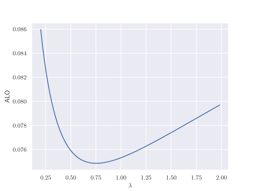
(a) ALO

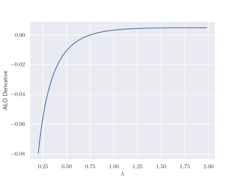
(b) ALO Derivative

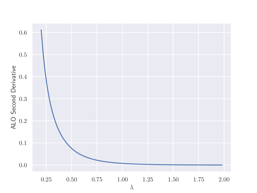
(c) ALO Second Derivative

Figure 1: ALO and derivatives for regularized logistic regression on the Breast Cancer data set. The regularizer is parameterized as $R_{\lambda}(\boldsymbol{\beta})=\lambda\left\|\boldsymbol{\beta}\right\|^{2}$.

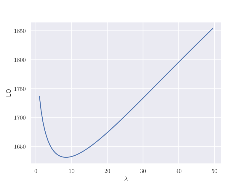
(a) LO

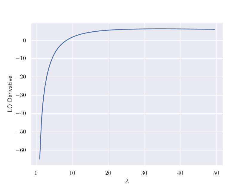
(b) LO Derivative

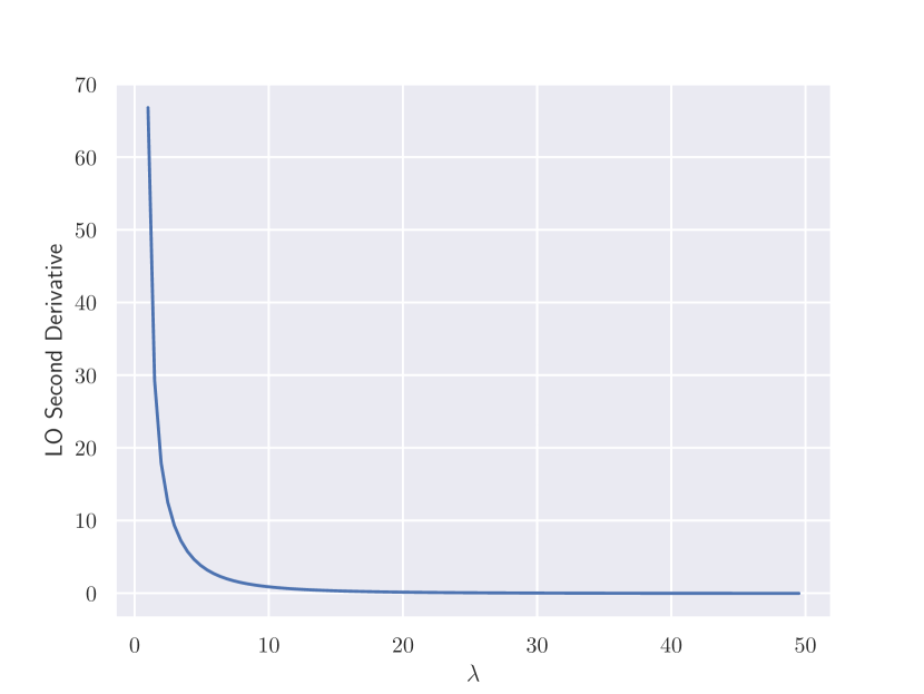
(c) LO Second Derivative

Figure 2: LO and derivatives for ridge regression on the Pollution data set. The regularizer is parameterized as $R_{\lambda}(\boldsymbol{\beta})=\lambda\left\|\boldsymbol{\beta}\right\|^{2}$.

6.2 Comparing ALO Optimization to Grid Search

We next compare hyperparameters found by ALO optimization to those found by grid search for the ridge regularizer. For ALO optimization, we use the Python package peak-engines available from https://github.com/rnburn/peak-engines; and for grid search, we use LogisticRegressionCV and RidgeCV from sklearn-0.23.1 with default settings. LogisticRegressionCV defaults to run a grid search using 5-fold cross-validation and 10 points of evaluation; RidgeCV defaults to run a grid search using LO and 3 points of evaluation. Figure 3 shows where the hyperparameters found by grid search and ALO optimization lie along the the LO and ALO curves.

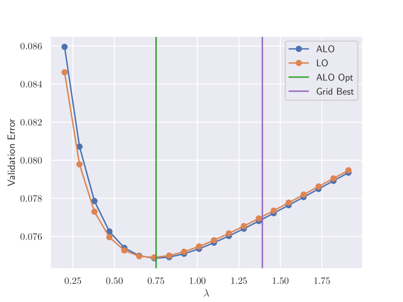
(a) Breast Cancer

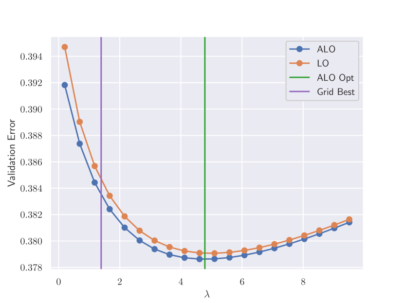
(b) Cleveland Heart

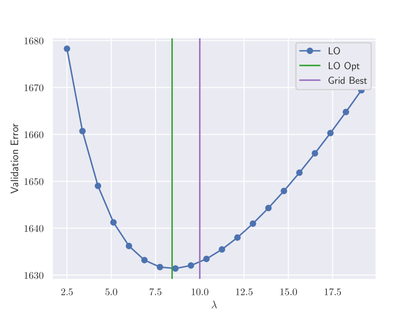
(c) Pollution

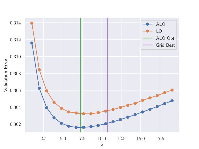
(d) Arcene

Figure 3: Plot of ALO and LO curves for ridge regression and regularized logistic regression on sample data sets. The green line shows the hyperparameter found by ALO optimization, and the purple line shows the hyperparameter found by grid search. The regularizer is parameterized as $R_{\lambda}(\boldsymbol{\beta})=\lambda\left\|\boldsymbol{\beta}\right\|^{2}$.

We additionally benchmark how long it takes ALO optimization and grid search to find hyperparameters on the sample data sets. Figure 4 shows the resulting durations measured in seconds.

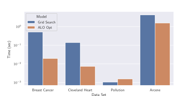
Figure 4: Benchmark showing how long ALO optimization and grid search take to find hyperparameters for ridge regression and regularized logistic regression on sample data sets. The times are averaged over 10 runs and shown on a logarithmic scale.

6.3 Fitting Models with Multiple Hyperparameters

To test ALO optimization with multiple hyperparameters, we fit logistic regression with a bridge regularizer (Fu, 1998) of the form $\lambda_{1}|\beta_{j}|^{\lambda_{2}}$, where $\lambda_{2}\geq 1$, to a 5-fold cross-validation of the Gisette data set. To ensure that $r_{j,\boldsymbol{\lambda}}$ has a continuous fourth derivative, we interpolate the regularizer with a polynomial when $|\beta_{j}|<\delta$ so that

$$r_{j,\boldsymbol{\lambda}}(\beta_{j})\triangleq\left\{\begin{array}[]{ll}\lambda_{1}|\beta_{j}|^{\lambda_{2}},&\mbox{if }|\beta_{j}|\geq\delta,\\ \lambda_{1}p_{\lambda_{2}}(|\beta_{j}|),&\mbox{if }|\beta_{j}|<\delta,\\ \end{array}\right.$$

where $p_{\lambda_{2}}(t)=a_{1}t^{2}+a_{2}t^{4}+a_{3}t^{5}+a_{4}t^{6}+a_{5}t^{7}$ and $\boldsymbol{a}$ is chosen so that $p_{\lambda_{2}}(\delta)$ matches $\delta^{\lambda_{2}}$ up to the fourth derivative. For our experiment, we use $\delta=0.01$. For comparison, we also fit logistic regression with ridge regularization. Table 2 shows the hyperparameters found for bridge regularization and ridge regularization and compares their performance on each cross-validation fold.

		Bridge				Ridge
Fold		$\lambda_{1}$	$\lambda_{2}$	Test Error		$\lambda$	Test Error
0		17.3	1.95	0.0698		19.1	0.0709
1		16.8	1.94	0.0581		18.7	0.0587
2		13.0	1.81	0.0667		18.3	0.0697
3		10.5	1.75	0.0677		16.5	0.0714
4		10.8	1.83	0.0639		14.4	0.0667
Mean				0.0652			0.0675

Table 2: Hyperparameters and performance of ALO optimization with logistic regression using bridge and ridge regularization on a 5-fold cross-validation of the Gisette data set. Test error is measured as the negative mean log-likelihood of the out-of-sample fold.

6.4 Comparing Derivatives with Finite Difference Approximations

While working out our equations for the ALO gradient and hessian, we made extensive use of finite difference approximations to validate our results. We present examples of finite difference testing for ridge regression and logistic regression using ridge and bridge regularization. We use the following finite difference approximation to the partial derivative of a function $g$:

$$\frac{\partial g}{\partial\lambda_{j}}\left(\boldsymbol{\lambda}\right)\approx\frac{g(\boldsymbol{\lambda}+h\boldsymbol{e}_{j})-g(\boldsymbol{\lambda})}{h},$$

where $h=0.000001$ and $\boldsymbol{e}_{j}$ denotes a $p$-demensional vector with the $j$^th entry equal to $1$ and all other entries equal to $0$. We approximate second derivatives by using the exact formula for the first derivative. Table 3 shows the finite difference derivative comparisons for ridge regression on the Pollution data set, Table 4 shows the comparisons for logistic regression on the Breast Cancer data set using ridge regularization, and Table 5 shows the comparisons for logistic regression on the Breast Cancer data set using bridge regularization.

		$\tfrac{\partial f}{\partial\lambda}$			$\tfrac{\partial^{2}f}{\partial\lambda^{2}}$
$\lambda$		Exact	Approx		Exact	Approx
0.01		-68.99	-69.03		-6879.30	-6879.27
0.05		-33.36	-33.39		-6195.24	-6195.10
0.10		-600.79	-600.81		-4371.80	-4371.59
1.00		-129.64	-129.63		137.56	137.56
2.00		-48.68	-48.68		65.14	65.14
5.00		59.95	59.95		18.15	18.15

Table 3: Comparison of LO derivatives and finite difference approximations for ridge regression on the Pollution data set using various values of $\lambda$. The regularizer is parameterized as $R_{\lambda}(\boldsymbol{\beta})=\lambda^{2}\left\|\boldsymbol{\beta}\right\|^{2}$.

		$\tfrac{\partial f}{\partial\lambda}$			$\tfrac{\partial^{2}f}{\partial\lambda^{2}}$
$\lambda$		Exact	Approx		Exact	Approx
0.01		-46.15	-45.68		3850.21	3837.37
0.05		-2.68	-2.68		119.42	119.33
0.10		-0.48	-0.48		8.31	8.29
1.00		-0.0064	-0.0064		0.035	0.035
2.00		0.015	0.015		0.0015	0.0015
5.00		0.015	0.015		-0.00041	-0.00041

Table 4: Comparison of ALO derivatives and finite difference approximations for regularized logistic regression on the Breast Cancer data set using various values of $\lambda$. The regularizer is parameterized as $R_{\lambda}(\boldsymbol{\beta})=\lambda^{2}\left\|\boldsymbol{\beta}\right\|^{2}$.

		$\tfrac{\partial f}{\partial\lambda_{1}}$			$\tfrac{\partial f}{\partial\lambda_{2}}$			$\tfrac{\partial^{2}f}{\partial\lambda_{1}^{2}}$			$\tfrac{\partial^{2}f}{\partial\lambda_{1}\partial\lambda_{2}}$			$\tfrac{\partial^{2}f}{\partial\lambda_{2}^{2}}$
$\lambda_{1}$	$\lambda_{2}$	Exact	Approx		Exact	Approx		Exact	Approx		Exact	Approx		Exact	Approx
0.05	0.75	-6.07	-6.07		-0.78	-0.78		146.24	146.19		8.90	8.89		1.04	1.04
0.05	1.00	-2.68	-2.68		-0.36	-0.36		119.42	119.33		10.20	10.19		1.28	1.28
0.05	1.25	-0.93	-0.93		-0.14	-0.14		50.87	50.70		4.35	4.35		0.56	0.56
0.25	0.75	-0.39	-0.39		-0.13	-0.13		-8.55	-8.57		-0.99	-1.00		0.019	0.018
0.25	1.00	-0.18	-0.18		-0.059	-0.059		0.89	0.89		0.13	0.13		0.088	0.088
0.25	1.25	-0.13	-0.13		-0.031	-0.031		0.82	0.82		0.22	0.22		0.11	0.11
1.00	0.75	0.0054	0.0054		-0.0077	-0.0077		0.047	0.047		0.013	0.013		0.032	0.033
1.00	1.00	0.0064	0.0064		-0.0021	-0.0021		0.035	0.035		0.0021	0.0021		0.020	0.020
1.00	1.25	0.0039	0.0039		0.00062	0.00061		-0.15	-0.16		-0.071	-0.072		-0.0065	-0.0068

Table 5: Comparison of ALO derivatives and finite difference approximations for regularized logistic regression on the Breast Cancer data set using various values of $\lambda_{1}$ and $\lambda_{2}$. The regularizer is parameterized as $r_{j,\boldsymbol{\lambda}}(\beta_{j})\triangleq\left\{\begin{array}[]{ll}\lambda_{1}^{2}|\beta_{j}|^{1+\lambda_{2}^{2}},&\mbox{if }|\beta_{j}|\geq\delta,\\ \lambda_{1}^{2}p_{\lambda_{2}}(|\beta_{j}|),&\mbox{if }|\beta_{j}|<\delta,\\ \end{array}\right.$ where $p$ and $\delta$ are defined as in Section 6.3.

7 Conclusion

In this paper, we demonstrated how to select hyperparameters by computing the gradient and hessian of ALO and applying a second-order optimizer to find a local minimum. The approach is applicable to a large class of commonly used models, including regularized logistic regression and ridge regression. We applied ALO optimization to fit regularized models to various real-world data sets. We found that when using a single-parameter regularizer, we were able to find hyperparameters with better LO values than standard grid search approaches and frequently were able to do so in less time. ALO optimization, furthermore, scales to handle multiple hyperparameters, and we demonstrated how it could be used to fit hyperparameters for bridge regularization.

Acknowledgments

We made use of the UCI Machine Learning Repository http://archive.ics.uci.edu/ml in our experiments.

Appendix A. Proof of Theorem 1

To derive the derivative of $\boldsymbol{\hat{\beta}}$, we observe that at the optimum of Equation 1 the gradient is zero:

$$\sum_{i=1}^{n}\dot{\ell}_{i}\left(u_{i}\right)\boldsymbol{x}_{i}+\nabla R_{\boldsymbol{\lambda}}(\boldsymbol{\hat{\beta}})=0.$$

Differentiating both sides of the equation gives us

$$\phantom{\Leftrightarrow}\frac{\partial}{\partial\lambda_{s}}\left(\sum_{i=1}^{n}\dot{\ell}_{i}\left(u_{i}\right)\boldsymbol{x}_{i}+\nabla R_{\boldsymbol{\lambda}}(\boldsymbol{\hat{\beta}})\right)=0$$

$$\Leftrightarrow\boldsymbol{H}\left(\frac{\partial\boldsymbol{\hat{\beta}}}{\partial\lambda_{s}}\right)+\frac{\partial\nabla R_{\boldsymbol{\lambda}}}{\partial\lambda_{s}}(\boldsymbol{\hat{\beta}})=0$$

$$\Leftrightarrow\frac{\partial\boldsymbol{\hat{\beta}}}{\partial\lambda_{s}}=-\boldsymbol{H}^{-1}\frac{\partial\nabla R_{\boldsymbol{\lambda}}}{\partial\lambda_{s}}(\boldsymbol{\hat{\beta}}).$$

For the derivative of $h_{i}$, we apply this formula for differentiating an inverse matrix:

$$\frac{d\boldsymbol{E}^{-1}}{dt}=-\boldsymbol{E}^{-1}\frac{d\boldsymbol{E}}{dt}\boldsymbol{E}^{-1}.$$

The other derivatives are derived as straightforward differentiations of their associated value formulas.

Appendix B. Proof of Theorem 2

For the second derivative of $\boldsymbol{\hat{\beta}}$, we derive

$$\frac{\partial^{2}\boldsymbol{\hat{\beta}}}{\partial\lambda_{s}\partial\lambda_{t}} =\frac{\partial}{\partial\lambda_{t}}\left[-\boldsymbol{H}^{-1}\frac{\partial\nabla R_{\boldsymbol{\lambda}}}{\partial\lambda_{s}}(\boldsymbol{\hat{\beta}})\right]$$

$$=\boldsymbol{H}^{-1}\frac{\partial\boldsymbol{H}}{\partial\lambda_{t}}\boldsymbol{H}^{-1}\frac{\partial\nabla R_{\boldsymbol{\lambda}}}{\partial\lambda_{s}}(\boldsymbol{\hat{\beta}})-\boldsymbol{H}^{-1}\frac{\partial}{\partial\lambda_{t}}\left(\frac{\partial\nabla R_{\boldsymbol{\lambda}}}{\partial\lambda_{s}}(\boldsymbol{\hat{\beta}})\right)$$

$$=-\boldsymbol{H}^{-1}\frac{\partial\boldsymbol{H}}{\partial\lambda_{t}}\frac{\partial\boldsymbol{\hat{\beta}}}{\partial\lambda_{s}}-\boldsymbol{H}^{-1}\frac{\partial}{\partial\lambda_{t}}\left(\frac{\partial\nabla R_{\boldsymbol{\lambda}}}{\partial\lambda_{s}}(\boldsymbol{\hat{\beta}})\right).$$

Now,

$$\left(\frac{\partial\boldsymbol{H}}{\partial\lambda_{t}}\right)\frac{\partial\boldsymbol{\hat{\beta}}}{\partial\lambda_{s}} =\left[\boldsymbol{X}^{\top}\frac{\partial\boldsymbol{A}}{\partial\lambda_{t}}\boldsymbol{X}+\frac{\partial\boldsymbol{W}}{\partial\lambda_{t}}\right]\frac{\partial\boldsymbol{\hat{\beta}}}{\partial\lambda_{s}}$$

$$=\!\begin{multlined}\boldsymbol{X}^{\top}\cdot\mathrm{vec}\left[\left\{\dddot{\ell}_{i}\left(u_{i}\right)\times\frac{\partial u_{i}}{\partial\lambda_{s}}\times\frac{\partial u_{i}}{\partial\lambda_{t}}\right\}_{i}\right]+\frac{\partial\nabla^{2}R_{\boldsymbol{\lambda}}}{\partial\lambda_{t}}(\boldsymbol{\hat{\beta}})\frac{\partial\boldsymbol{\hat{\beta}}}{\partial\lambda_{s}}\\ +\mathrm{vec}\left[\left\{\dddot{r}_{j,\boldsymbol{\lambda}}(\hat{\beta}_{j})\times\frac{\partial\hat{\beta}_{j}}{\partial\lambda_{s}}\times\frac{\partial\hat{\beta}_{j}}{\partial\lambda_{t}}\right\}_{j}\right]\quad\mbox{and}\end{multlined}\boldsymbol{X}^{\top}\cdot\mathrm{vec}\left[\left\{\dddot{\ell}_{i}\left(u_{i}\right)\times\frac{\partial u_{i}}{\partial\lambda_{s}}\times\frac{\partial u_{i}}{\partial\lambda_{t}}\right\}_{i}\right]+\frac{\partial\nabla^{2}R_{\boldsymbol{\lambda}}}{\partial\lambda_{t}}(\boldsymbol{\hat{\beta}})\frac{\partial\boldsymbol{\hat{\beta}}}{\partial\lambda_{s}}\\ +\mathrm{vec}\left[\left\{\dddot{r}_{j,\boldsymbol{\lambda}}(\hat{\beta}_{j})\times\frac{\partial\hat{\beta}_{j}}{\partial\lambda_{s}}\times\frac{\partial\hat{\beta}_{j}}{\partial\lambda_{t}}\right\}_{j}\right]\quad\mbox{and}$$

$$\frac{\partial}{\partial\lambda_{t}}\left(\frac{\partial\nabla R_{\boldsymbol{\lambda}}}{\partial\lambda_{s}}(\boldsymbol{\hat{\beta}})\right) =\frac{\partial\nabla^{2}R_{\boldsymbol{\lambda}}}{\partial\lambda_{s}}(\boldsymbol{\hat{\beta}})\frac{\partial\boldsymbol{\hat{\beta}}}{\partial\lambda_{t}}+\frac{\partial\nabla R_{\boldsymbol{\lambda}}}{\partial\lambda_{s}\partial\lambda_{t}}(\boldsymbol{\hat{\beta}}).$$

Combining the equations, the second derivative of $\boldsymbol{\hat{\beta}}$ becomes

$$\frac{\partial^{2}\boldsymbol{\hat{\beta}}}{\partial\lambda_{s}\partial\lambda_{t}}=-\boldsymbol{H}^{-1}\boldsymbol{X}^{\top}\cdot\mathrm{vec}\left[\left\{\dddot{\ell}_{i}\left(u_{i}\right)\times\frac{\partial u_{i}}{\partial\lambda_{s}}\times\frac{\partial u_{i}}{\partial\lambda_{t}}\right\}_{i}\right]\\ -\boldsymbol{H}^{-1}\frac{\partial\nabla^{2}R_{\boldsymbol{\lambda}}}{\partial\lambda_{s}}(\boldsymbol{\hat{\beta}})\frac{\partial\boldsymbol{\hat{\beta}}}{\partial\lambda_{t}}-\boldsymbol{H}^{-1}\frac{\partial\nabla^{2}R_{\boldsymbol{\lambda}}}{\partial\lambda_{t}}(\boldsymbol{\hat{\beta}})\frac{\partial\boldsymbol{\hat{\beta}}}{\partial\lambda_{s}}-\boldsymbol{H}^{-1}\frac{\partial\nabla R_{\boldsymbol{\lambda}}}{\partial\lambda_{s}\partial\lambda_{t}}(\boldsymbol{\hat{\beta}})\\ -\boldsymbol{H}^{-1}\cdot\mathrm{vec}\left[\left\{\dddot{r}_{j,\boldsymbol{\lambda}}(\hat{\beta}_{j})\times\frac{\partial\hat{\beta}_{j}}{\partial\lambda_{s}}\times\frac{\partial\hat{\beta}_{j}}{\partial\lambda_{t}}\right\}_{j}\right].$$

For the second derivative of $h_{i}$, we derive

$$\frac{\partial^{2}h_{i}}{\partial\lambda_{s}\partial\lambda_{t}} =\frac{\partial}{\partial\lambda_{t}}\left(-\boldsymbol{x}_{i}^{\top}\boldsymbol{H}^{-1}\frac{\partial\boldsymbol{H}}{\partial\lambda_{s}}\boldsymbol{H}^{-1}\boldsymbol{x}_{i}\right)$$

$$=\!\begin{multlined}\boldsymbol{x}_{i}^{\top}\boldsymbol{H}^{-1}\frac{\partial\boldsymbol{H}}{\partial\lambda_{t}}\boldsymbol{H}^{-1}\frac{\partial\boldsymbol{H}}{\partial\lambda_{s}}\boldsymbol{H}^{-1}\boldsymbol{x}_{i}+\boldsymbol{x}_{i}^{\top}\boldsymbol{H}^{-1}\frac{\partial\boldsymbol{H}}{\partial\lambda_{s}}\boldsymbol{H}^{-1}\frac{\partial\boldsymbol{H}}{\partial\lambda_{t}}\boldsymbol{H}^{-1}\boldsymbol{x}_{i}\\ -\boldsymbol{x}_{i}^{\top}\boldsymbol{H}^{-1}\frac{\partial^{2}\boldsymbol{H}}{\partial\lambda_{s}\partial\lambda_{t}}\boldsymbol{H}^{-1}\boldsymbol{x}_{i}\end{multlined}\boldsymbol{x}_{i}^{\top}\boldsymbol{H}^{-1}\frac{\partial\boldsymbol{H}}{\partial\lambda_{t}}\boldsymbol{H}^{-1}\frac{\partial\boldsymbol{H}}{\partial\lambda_{s}}\boldsymbol{H}^{-1}\boldsymbol{x}_{i}+\boldsymbol{x}_{i}^{\top}\boldsymbol{H}^{-1}\frac{\partial\boldsymbol{H}}{\partial\lambda_{s}}\boldsymbol{H}^{-1}\frac{\partial\boldsymbol{H}}{\partial\lambda_{t}}\boldsymbol{H}^{-1}\boldsymbol{x}_{i}\\ -\boldsymbol{x}_{i}^{\top}\boldsymbol{H}^{-1}\frac{\partial^{2}\boldsymbol{H}}{\partial\lambda_{s}\partial\lambda_{t}}\boldsymbol{H}^{-1}\boldsymbol{x}_{i}$$

$$=2\boldsymbol{x}_{i}^{\top}\boldsymbol{H}^{-1}\frac{\partial\boldsymbol{H}}{\partial\lambda_{s}}\boldsymbol{H}^{-1}\frac{\partial\boldsymbol{H}}{\partial\lambda_{t}}\boldsymbol{H}^{-1}\boldsymbol{x}_{i}-\boldsymbol{x}_{i}^{\top}\boldsymbol{H}^{-1}\frac{\partial^{2}\boldsymbol{H}}{\partial\lambda_{s}\partial\lambda_{t}}\boldsymbol{H}^{-1}\boldsymbol{x}_{i},$$

$$\frac{\partial^{2}\boldsymbol{H}}{\partial\lambda_{s}\partial\lambda_{t}} =\frac{\partial}{\partial\lambda_{t}}\left(\boldsymbol{X}^{\top}\frac{\partial\boldsymbol{A}}{\partial\lambda_{s}}\boldsymbol{X}+\frac{\partial\boldsymbol{W}}{\partial\lambda_{s}}\right)$$

$$=\boldsymbol{X}^{\top}\frac{\partial^{2}\boldsymbol{A}}{\partial\lambda_{s}\partial\lambda_{t}}\boldsymbol{X}+\frac{\partial^{2}\boldsymbol{W}}{\partial\lambda_{s}\partial\lambda_{t}},\mbox{ and}$$

$$\left(\frac{\partial^{2}\boldsymbol{W}}{\partial\lambda_{s}\partial\lambda_{t}}\right)_{jj} =\frac{\partial}{\partial\lambda_{t}}\left(\frac{\partial\ddot{r}_{j,\boldsymbol{\lambda}}}{\partial\lambda_{s}}(\hat{\beta}_{j})+\dddot{r}_{j,\boldsymbol{\lambda}}(\hat{\beta}_{j})\times\frac{\partial\hat{\beta}_{j}}{\partial\lambda_{s}}\right)$$

$$=\!\begin{multlined}\frac{\partial^{2}\ddot{r}_{j,\boldsymbol{\lambda}}}{\partial\lambda_{s}\partial\lambda_{t}}(\hat{\beta}_{j})+\frac{\partial\dddot{r}_{j,\boldsymbol{\lambda}}}{\partial\lambda_{s}}(\hat{\beta}_{j})\times\frac{\partial\hat{\beta}_{j}}{\partial\lambda_{t}}+\frac{\partial\dddot{r}_{j,\boldsymbol{\lambda}}}{\partial\lambda_{t}}(\hat{\beta}_{j})\times\frac{\partial\hat{\beta}_{j}}{\partial\lambda_{s}}\\ +\dddot{r}_{j,\boldsymbol{\lambda}}(\hat{\beta}_{j})\times\frac{\partial^{2}\hat{\beta}_{j}}{\partial\lambda_{s}\partial\lambda_{t}}+\ddddot{r}_{j,\boldsymbol{\lambda}}(\hat{\beta}_{j})\times\frac{\partial\hat{\beta}_{j}}{\partial\lambda_{s}}\times\frac{\partial\hat{\beta}_{j}}{\partial\lambda_{t}}.\end{multlined}\frac{\partial^{2}\ddot{r}_{j,\boldsymbol{\lambda}}}{\partial\lambda_{s}\partial\lambda_{t}}(\hat{\beta}_{j})+\frac{\partial\dddot{r}_{j,\boldsymbol{\lambda}}}{\partial\lambda_{s}}(\hat{\beta}_{j})\times\frac{\partial\hat{\beta}_{j}}{\partial\lambda_{t}}+\frac{\partial\dddot{r}_{j,\boldsymbol{\lambda}}}{\partial\lambda_{t}}(\hat{\beta}_{j})\times\frac{\partial\hat{\beta}_{j}}{\partial\lambda_{s}}\\ +\dddot{r}_{j,\boldsymbol{\lambda}}(\hat{\beta}_{j})\times\frac{\partial^{2}\hat{\beta}_{j}}{\partial\lambda_{s}\partial\lambda_{t}}+\ddddot{r}_{j,\boldsymbol{\lambda}}(\hat{\beta}_{j})\times\frac{\partial\hat{\beta}_{j}}{\partial\lambda_{s}}\times\frac{\partial\hat{\beta}_{j}}{\partial\lambda_{t}}.$$

We omit the steps for the other derivatives as they are straightforward.

References

- Allen (1974) D. M. Allen. The relationship between variable selection and data augmentation and a method for prediction. Technometrics, 16:125–127, 1974.
- Bengio (2000) Y. Bengio. Gradient-based optimization of hyperparameters. Neural Computation, 12(8):1889–1900, 2000.
- Bergstra and Bengio (2012) J. Bergstra and Y. Bengio. Random search for hyper-parameter optimization. Journal of Machine Learning Research, 13:281–305, 2012.
- Do et al. (2008) C. B. Do, D. A. Woods, A. Y. Ng. Efficient multiple hyperparameter learning for log-linear models. Advances in Neural Information Processing Systems, 20:377–384, 2008.
- Fu (1998) W. J. Fu. Penalized regression: the bridge versus the lasso. Journal of Computational and Graphical Statistics, 7:397–416, 1998.
- McDonald and Schwing (1973) G. C. McDonald and R. C. Schwing. Instabilities of regression estimates relating air pollution to mortality. Technometrics, 15:463–481, 1973.
- Moré and Sorensen (1983) J. J. Moré and D. C. Sorensen. Computing a trust region step. SIAM Journal on Scientific and Statistical Computing, 4(3):553–572, 1983.
- Nocedal and Wright (1999) J. Nocedal and S. J. Wright. Numerical Optimization. Springer Series in Operations Research and Financial Engineering. Springer, Second edition, 1999.
- Rad and Maleki (2020) K. R. Rad and A. Maleki. A scalable estimate of the extra-sample prediction error via approximate leave-one-out. ArXiv:1801.10243v4, 2020.
- Rad et al. (2020) K. R. Rad, W. Zhou, A. Maleki. Error bounds in estimating the out-of-sample prediction error using leave-one-out cross validation in high-dimensions. ArXiv:2003.01770v1, 2020.
- Sorensen (1982) D. C. Sorensen. Newton’s method with a model trust region modification. SIAM Journal on Numerical Analysis, 19(2):409–426, 1982.