ClickTrain: Efficient and Accurate End-to-End Deep Learning Training via Fine-Grained Architecture-Preserving Pruning

Abstract.

Convolutional neural networks (CNNs) are becoming increasingly deeper, wider, and non-linear because of the growing demand on prediction accuracy and analysis quality. The wide and deep CNNs, however, require a large amount of computing resources and processing time. Many previous works have studied model pruning to improve inference performance, but little work has been done for effectively reducing training cost. In this paper, we propose ClickTrain: an efficient and accurate end-to-end training and pruning framework for CNNs. Different from the existing pruning-during-training work, ClickTrain provides higher model accuracy and compression ratio via fine-grained architecture-preserving pruning. By leveraging pattern-based pruning with our proposed novel accurate weight importance estimation, dynamic pattern generation and selection, and compiler-assisted computation optimizations, ClickTrain generates highly accurate and fast pruned CNN models for direct deployment without any extra time overhead, compared with the baseline training. ClickTrain also reduces the end-to-end time cost of the pruning-after-training method by up to 2.3$\times$ with comparable accuracy and compression ratio. Moreover, compared with the state-of-the-art pruning-during-training approach, ClickTrain provides significant improvements both accuracy and compression ratio on the tested CNN models and datasets, under similar limited training time.

1. Introduction

Deep neural networks (DNNs) such as CNNs have rapidly evolved to the state-of-the-art technique for many artificial intelligence (AI) tasks in various science and technology areas, such as image and vision recognition (Simonyan and Zisserman, 2014), recommender systems (Wang et al., 2015), natural language processing (Collobert and Weston, 2008). DNNs contain millions of parameters in an unparalleled representation, which is efficient for modeling complexity nonlinearities. Many works (Krizhevsky et al., 2012; Szegedy et al., 2015; He et al., 2016) have suggested that using either deeper or wider DNNs is an effective way to improve analysis quality, and in fact many recent DNNs have gone significantly deeper and/or wider (Wang et al., 2018b; Jin et al., 2019). For instance, OpenAI recently published their new DNN-based NLP model GPT-3 (Brown et al., 2020) with 175 billion parameters, which is the largest NLP model that is ever trained. Compared with its predecessor GPT-2, GPT-3 expands the capacity by three orders of magnitudes without significant modification to the model architecture, instead just adopting deeper and wider layers (Brown et al., 2020).

The ever-increasing scale and complexity of the networks with large-scale training datasets such as ImageNet-2012 (Large Scale Visual Recognition Challenge, 2020) are bringing more and more challenges to the cost of DNN training, which requires large amounts of computations and resources such as memory, storage, and I/O (Wang et al., 2018b; Ma et al., 2018; Zhang et al., 2020, 2021a; Zhang et al., 2021b). Previous works have also tried some optimization methods to try to overcome these challenges (Ding et al., 2017; Roy et al., 2018; Wang et al., 2018a; Ding et al., 2018; Li et al., 2019; Geng et al., 2019). Moreover, designing new DNN architectures and training algorithms for various AI tasks require numerous trial-and-error and fine-tuning processes, which makes the training cost issue worse and computing resources scarce.

Model pruning is a widely used approach to reduce the number of DNN weights, which can effectively reduce the computation and storage costs and increase the inference performance, especially for resource-limited platforms, such as mobile, edge, and IoT devices (Cai et al., 2020; Li et al., 2021; Zhao et al., 2020; Niu et al., 2020a). Many model pruning works have been proposed for improving the performance and energy efficiency of DNN inference (Molchanov et al., 2016; Han et al., 2016; Luo et al., 2017; Yang et al., 2017; Yu et al., 2018; Yuan et al., 2019b; Ma et al., 2019c; Ma et al., 2020c). A typical procedure to prune a DNN model consists of training a model to high accuracy, pruning the well-trained model, and fine-tuning the pruned model. However, this procedure (called pruning-after-training or PAT) often requires a well-trained model and a trial-and-error process with domain expertise, which is typically very time-consuming. For example, state-of-the-art PAT-based methods (Ma et al., 2020b, a) incorporate the alternating direction method of multipliers (ADMM) into the pruning process to achieve high compression ratio and accuracy, but they almost triple the overall training time.

Considering the weights of DNN models are gradually sparsified during training, combining the pruning and training phases together (called pruning-during-training or PDT) is a promising way to significantly reduce the end-to-end time cost and conserve computing resources. However, only few work has investigated how to prune DNN models during training while still achieving highly accurate and fast pruned models that can be directly deployed.

Recently, a state-of-the-art work PruneTrain (Lym et al., 2019) studied how to perform CNN pruning during training. PruneTrain adopts a group-lasso regularization ($\ell_{1}$-based regularization) (Meier et al., 2008) to gradually force a group of model weights with small magnitudes to zero and periodically reconfigure the CNN architecture (e.g., reducing the number of layers) during training, leading to lower computation and higher performance. However, in reality, adaptively changing the original network architecture may result in severe loss of accuracy, which cannot be compensated for by performing more training batches. Thus, how to design a PDT-based method to significantly reduce the end-to-end time while still maintaining the network architecture for high accuracy remains an open question.

In this paper, we propose ClickTrain—a fast and accurate integrated framework for CNN training and pruning—which significantly reduces the end-to-end time. We develop a series of algorithm-level and system-level optimizations for ClickTrain to achieve high computation efficiency toward highly accurate and fast pruned models for inference. The key insights explored for algorithm-level optimization include: the position of the most important weight in each convolution kernel is relatively stable after certain training batches, and the important weights tend to be adjacent to each other. Thus, we propose a fine-grained architecture-preserving pruning approach based on pattern-based pruning (will be discussed in §2.1), which can preserve the original training accuracy under a higher compression ratio. Moreover, our optimized pattern-based pruning creates multiple opportunities for system-level optimization such as sparse convolution acceleration and communication (Allreduce) optimization for weight update assisted by compiler so that the time overhead introduced by our proposed regularization can be mitigated. To the best of our knowledge, our paper is the first work to study how to design a PDT-based approach for effectively reducing the end-to-end time cost while achieving very high accuracy and compression ratio of pruned models. The main contributions are listed below:

• Instead of commonly used weight selection methods based on magnitude, we incorporate a state-of-the-art weight importance estimation approach to select the desired patterns from a generated candidate pattern pool. Moreover, we propose methods to gradually generate the candidate patterns (called dynamic pattern pool generation) and adaptively finalize the patterns and unimportant kernels.

• We propose a modified group-lasso regularization to replace the expensive ADMM method for pattern-based pruning.

• We propose multiple system-level optimizations including fast sparse matrix format conversion, pattern-accelerated sparse convolution, pattern-based communication optimization, and compiler-assisted optimized code generation, to significantly accelerate ClickTrain by leveraging finalized pattern sparsity during the training.

• We compare ClickTrain with state-of-the-art PAT-/PDT-based methods. Experiments illustrate that ClickTrain can generate highly accurate and fast pruned models for direct deployment without any extra time overhead or even faster, compared with the baseline training. Meanwhile, ClickTrain significantly reduces the training time of PAT-based approaches by up to about 2.3$\times$ with comparable accuracy and compression ratio, and improves the accuracy and compression ratio by up to 1.8% and 4.9$\times$ over PruneTrain.

The rest of the paper is organized as follows. We present background information in §2. We discuss our research motivation and challenges in §3. We describe our algorithm-level design and system-level optimizations of ClickTrain in §4 and §5, respectively. We present our evaluation results in §6. We discuss related work and conclude our work in §7 and §8.

2. Background

2.1. DNN Model Pruning

Weight pruning for DNN model compression has been well studied in recent years. Below are three main methods.

Non-Structured Pruning.

The non-structured pruning methods studied in the previous works (Zhang et al., 2018) aim to heuristically prune the redundant weights on arbitrary locations. This leads to irregular weight distribution and inevitably introduces extra indices to store the locations of pruned weights. Eventually, this drawback limits performance acceleration (Dong et al., 2020; Ma et al., 2021).

Structured Pruning.

To overcome these limitations, structured pruning has been investigated in the recent studies (He et al., 2018; He et al., 2017; Lym et al., 2019; Yuan et al., 2019a; Li et al., 2020). They proposed to prune the entire filters, channels to maintain the structural regularity of the weight matrices after pruning. By taking advantage of the regular shapes of the pruned weight matrices, structured pruning becomes more hardware-friendly and achieves much higher speedups (Ma et al., 2019b). However, due to the constraints of its coarse-grained pruning, structured pruning suffers from high accuracy loss.

Fined-Grained Pattern-Based Pruning.

The state-of-the-art pruning work (Niu et al., 2020b) proposes a fine-grained pattern-based pruning scheme, which generates an intermediate sparsity type between non-structured pruning and structured pruning. They prune a fixed number of weights in each convolution kernel (e.g., pruning 5 weights out of 9 weights in a 3$\times$3 convolution kernel), and make the remaining weights to be concentrated in a certain area to form specific kernel patterns (called pattern sparsity), as shown in Figure 1 (left). However, the compression ratio that is achieved by pattern sparsity is limited. So, they further propose to exploit the inter-convolution kernel sparsity, which aims to remove some unimportant kernels (called connectivity sparsity), as shown in Figure 1 (right). It can further enlarge the weights compression rate while reducing the convolution operations in CNNs.

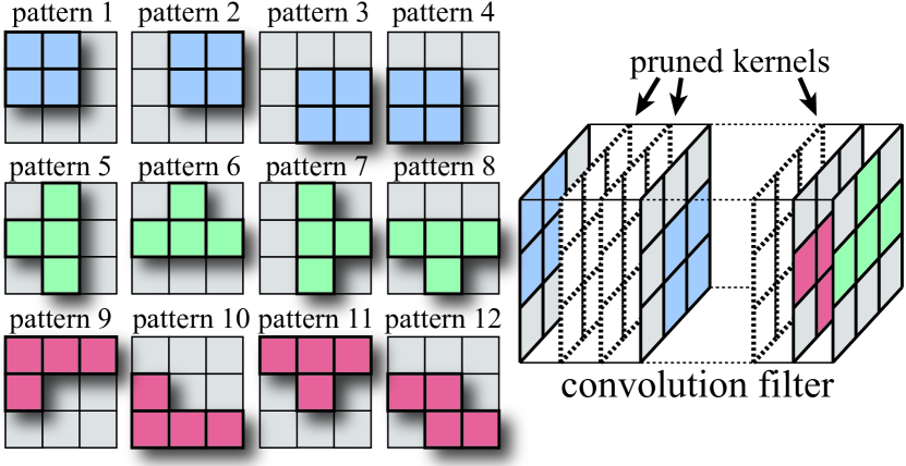
Figure 1. Pattern-based pruning with pruned kernels.

The pattern-based pruning emphasizes exploiting locality in layer-wise computation, which is prevalent and widely reflected in the domains like human visual systems (Freeman and Adelson, 1991). Moreover, this approach is more flexible that leads to a higher model accuracy compared to the prior coarse-grained filter/channel pruning schemes (Yuan et al., 2019a; Lym et al., 2019). Overall, a fine-grained pattern-based pruning approach, as state-of-the-art pruning scheme, considering both pattern and connectivity sparsity can leverage the advantages of non-structured and structured pruning to make the trade-off among regularity, accuracy, and compression ratio.

2.2. Pruning-after-training (PAT) Versus Pruning-during-training (PDT)

GBN (You et al., 2019b), GAL (Lin et al., 2019) and DCP (Zhuang et al., 2018) are three state-of-the-art PAT-based approaches. GBN and GAL mainly focus on pruning filters. DCP accelerates the CNN inference via channel pruning. However, all of them must need well-trained models to converge to an accurate pruned model with high compression ratio, which suffers from high time cost, compared with PDT-based approaches.

PruneTrain (Lym et al., 2019) is a state-of-the-art PDT-based approach. The work observed that when pruning with group-lasso regularization, once a group of model weights are penalized close to zero, their magnitudes are typically impossible to recover during the rest of the training process. Based on this, PruneTrain periodically removes the small weights and change the network architecture and hence gradually reduces the training cost toward high compression ratio and accuracy. Moreover, NeST (Dai et al., 2019) and TAS (Dong and Yang, 2019) are two state-of-the-art methods attempting to search the best-fit pruned network architecture during training (can be seen as PDT-based methods), but they suffer from extremely high time cost.

3. Motivation and Challenges

3.1. Limitations of Existing PDT-based Method

The state-of-the-art PDT-based approach PruneTrain (Lym et al., 2019) integrates the structured pruning with group-lasso regularization ($\ell_{1}$-based regularization) (Meier et al., 2008) into the training phase, which is designed to prune as many channels, filters, and layers as possible to acquire a compact architecture with relatively high training performance. However, there are two major challenges to deploy Prunetrain for training large neural networks on a variety of architectures: inferior validation accuracy and large storage overhead.

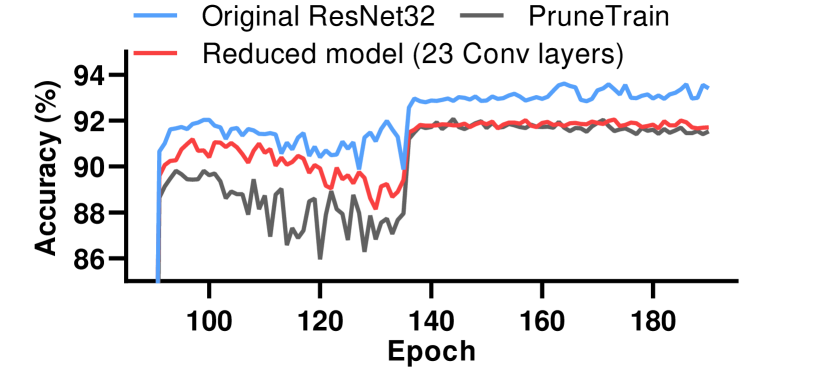
Figure 2. Achieved accuracies with three strategies: full training, Prunetrain, training on reduced architecture.

Inferior Validation Accuracy. PruneTrain saves the training floating-point operations (FLOPs) by drastically reconfiguring the original network architectures (e.g., reducing the depth), resulting in a notable accuracy loss for many network architectures. For example, PruneTrain can save $53\%$ training FLOPs and $66\%$ inference FLOPs (i.e., about $2.2\times$ compression ratio) but cause $1.8\%$ accuracy drop for ResNet-32 on the CIFAR-10 dataset. Moreover, for demonstration purposes, we compare three different training strategies on ResNet-32, including (1) normal full training from scratch on the original ResNet-32 model, (2) PruneTrain for training the original 34-layer ResNet, and (3) training from scratch using an identical network structure as the one generated from PruneTrain (i.e., 23 CONV layers). As shown in Figure 2, PruneTrain achieves a lower model accuracy compared to training on the reduced model, but both of them cannot reach the expected accuracy of the original ResNet-32 network, even though we train for an extra of 1,000 epochs. This experiment illustrates that the accuracy is highly relevant to network architectures. Moreover, studies (Liu et al., 2018; Dong and Yang, 2019; He et al., 2016; Elsken et al., 2018) demonstrate that the model accuracy is highly relevant to network architecture, thus, we conclude that aggressively preserving the original architecture is critical to prevent a notable accuracy drop.

Large Storage Overhead. One major purpose of pruning large-scale neural networks is to facilitate their deployments in resource-constrained computing platforms which suffer from limited storage capacity and computing power. Thus, to realistically alleviate the storage and computation burden, pruning must provide a high compression ratio. However, PruneTrain can only provide up to $3\times$ compression ratio (e.g., $2.2\times$ for ResNet-32) (Lym et al., 2019), which is far below the expectation.

Therefore, these issues motivate us to develop a solution that provides three-dimensional optimizations: high training efficiency, high compression ratio, and high model accuracy.

3.2. Challenges of Pattern-based Pruning in Training

Recent works (Ma et al., 2020b; Niu et al., 2020b) have applied pattern-based pruning techniques for improving inference efficiency. However, these inference-focused strategies will pose several challenges to reach our three optimization objectives.

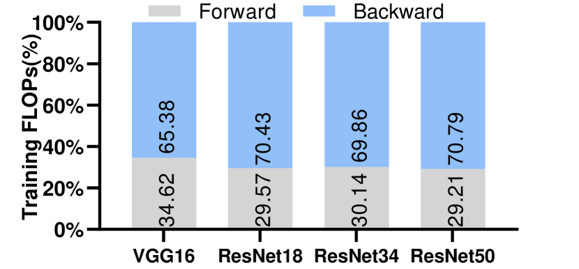
Figure 3. Percentage of floating-point operations in forward and backward phases with different CNN models.

Issues of Existing Pattern Pruning Algorithms. There are three main issues of the existing pattern-based pruning algorithms (Niu et al., 2020b; Dong et al., 2020): (1) The existing algorithms select pattern for each kernel via estimating weight importance based on magnitude. However, this estimation approach requires a well-trained model, whose weights will not change dramatically, which is not true for training from scratch. (2) The existing algorithms predefine the candidate patterns for all kernels and statically select the best-fit pattern for each kernel. But for pruning during training, static patterns may not work properly, resulting in a significant loss of accuracy. (3) The existing algorithms typically with ADMM-based methods are very time-consuming and not applicable for training acceleration.

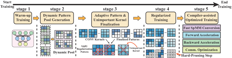
Figure 4. Overview of our proposed fast and accurate end-to-end deep learning training framework ClickTrain.

Lack of Training Efficiency Optimization. The computation efficiency optimizations proposed by existing works (Niu et al., 2020b; Dong et al., 2020) for pattern-based pruning cannot be directly applied to our training framework. This is mainly because of two reasons. On one hand, the existing pattern-based acceleration techniques (Dong et al., 2020; Niu et al., 2020b) are designed for accelerating inference (i.e., forward phase) instead of training (including both forward and back phases). However, based on our profiling result as shown in Figure 3, backward phase can consume more than 70% of the overall training FLOPs. On the other hand, the existing pattern-based optimizations (Niu et al., 2020b) are based on accelerating numerous convolution operations on embedded systems due to limited memory capacity. However, efficient training on advanced datacenter architectures relies on high-performance general matrix-matrix multiplication (GEMM) rather than a large number of convolutions, in order to leverage the high throughput of accelerators such as GPUs. Thus, there is an urgent need for an effective method to take advantage of pattern-based pruning to improve the GEMM-based convolution computation efficiency.

Overall, these challenges demand a novel solution that can provide both algorithm-level and system-level supports for fast and accurate end-to-end training toward our three objectives.

4. Algorithm-Level Design of ClickTrain

In this section, we propose our novel PDT-based framework called ClickTrain. The overall framework flow is shown in Figure 4, which consists of five stages. In this section, we focus on the algorithm-level design of ClickTrain (used in stage 2 to stage 4) mainly for quickly obtaining the model with desired pattern-based sparsity. We first propose our pattern selection using weight importance estimation. Next, we propose our methods to dynamically build up the pattern candidates and adaptively finalize the patterns and unimportant kernels. After that, we describe our modified group-lasso regularization to accurately penalize the weights outside of the selected patterns and the unimportant kernels.

4.1. Pattern and Kernel Selection Criterion

Weight importance estimation. The key consideration in the pattern-based pruning is to select the best-fit pattern for each kernel after appropriately designing the patterns. The previous methods (Ma et al., 2019a; Niu et al., 2020b) determine the importance of a certain weight based on its magnitude, which requires a well-trained CNN model whose weights will not change dramatically and well distributed after pruning the redundant filters. However, it is not feasible to accurately determine the importance of a certain weight only based on its weight magnitude during training from scratch because the weights in a not well-trained model will change greatly, especially in the early training. Therefore, we propose to estimate the importance of patterns by further considering gradient information and to select the most important pattern for each kernel in the pruning.

For a given CNN with $L$ convolutional layers, let $W^{(\ell)}$ ($1\leq\ell\leq L$) denote the collection of weights for all the kernels in convolutional layer $\ell$, which forms a 4-D tensor $W^{(\ell)}\in R^{F_{\ell}\times C_{\ell}\times H_{\ell}\times S_{\ell}}$, where $F_{\ell}$, $C_{\ell}$, $H_{\ell}$, $S_{\ell}$ are the dimensions for the axes of filter, channel, spatial height, spatial width, respectively. As suggested by (Molchanov et al., 2019), for a weight $w_{m}\in W^{(\ell)}$, its importance can be estimated by $(g_{m}w_{m})^{2}$, where $g_{m}=\frac{\partial E(W,D)}{\partial w_{m}}$ is the gradient of the weight $w_{m}$. Here $E(W,D)$ is the loss function on the dataset $D$. In addition, $W$ represents the collection of all 4-D weight tensors for $L$ convolutional layers.

A pattern $p_{i}$ (where $p_{i}\in B$ is the $i$-th pattern from the candidate pattern pool $B=\begin{Bmatrix}p_{1},p_{2},\cdots,p_{N}\end{Bmatrix}$) can be viewed as a mask to prune specific weights within a kernel. The remaining weights of the kernel form a certain pattern. Thus, we can estimate the importance score of a pattern $p_{i}$ by combining the importance scores of all the remaining weights. We will discuss how to gradually generate the pattern pool in the next section. The patterns corresponding to the convolutional layer $\ell$ also form a 4-D tensor $P^{(\ell)}\in R^{F_{\ell}\times C_{\ell}\times H_{\ell}\times S_{\ell}}$, where $P^{(\ell)}_{\smash{f_{\ell},c_{\ell},:,:}}\in B$. The importance score of $p_{i}$ is estimated as

(1) $$\textstyle t_{:,:}=G^{(\ell)}_{f_{\ell},c_{\ell},:,:}\odot W^{(\ell)}_{f_{\ell},c_{\ell},:,:}\odot p_{i},\;\;I_{p_{i}}=\sum_{h_{\ell}}^{H_{\ell}}\sum_{s_{\ell}}^{S_{\ell}}(t_{h_{\ell}\times s_{\ell}})^{2}$$

where $G^{(\ell)}$ denotes the 4-D gradient tensor corresponding to $W^{(\ell)}$ and $\odot$ is the element-wise product (a.k.a, Hadamard product). After assessing the importance of all the patterns for a kernel, we can choose the pattern with the highest estimated importance score as the best-fit pattern for this kernel.

In addition, to further enlarge the sparsity, we also need to determine the unimportant kernels and directly prune them (i.e., connectivity sparsity). We adopt the following equation to estimate the importance score of a kernel $k_{i}\in W^{(\ell)}$.

(2) $$\textstyle t_{:,:}=G^{(\ell)}_{f_{\ell},c_{\ell},:,:}\odot W^{(\ell)}_{f_{\ell},_{\ell},:,:},\;\;I_{k_{i}}=\sum_{h_{\ell}}^{H_{\ell}}\sum_{s_{\ell}}^{S_{\ell}}(t_{h_{\ell}\times s_{\ell}})^{2}$$

The reason why we integrate gradient to estimate the importance is if a certain weight whose magnitude and gradient are small, it will very likely keep the small value in the following training process because the backpropagation tends not to update its value dramatically. Therefore, we can treat it as an unimportant weight and penalize such weights during training to push it to become smaller and smaller (less and less important). Eventually, we can prune it with no hurt to the final accuracy. The computation cost of Equation (1) and (2) are relatively low, since the gradient $G^{(\ell)}$ can be acquired in the backward-propagation stage, which can be naturally implemented in most of the deep learning frameworks (Abadi et al., 2016; Paszke et al., 2019). Moreover, the number of candidate patterns is limited to a relatively small number (will be discussed later).

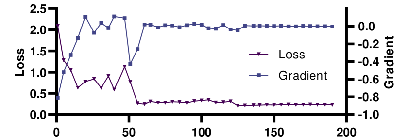
Figure 5. Loss & gradient in training ResNet-32 on CIFAR-10.

Pattern and kernel selection. The weights and gradients would change greatly during the first few epochs of training CNN. On one hand, estimating the weight importance earlier can help us remove these unimportant weights sooner, thereby reducing the overall training time. On the other hand, estimating the importance of weights prematurely will lead to inaccurate estimations and ultimately cause a significant accuracy drop. Later estimation does help to improve the pruning accuracy but would cost more training epochs. Therefore, when we should apply the formulas above to accurately assess the weight importance is a challenge to address. After a series of empirical evaluation, we conclude that the derivative of the loss function on epochs can be used as a good indicator to solve this problem. In particular, when this value is less than a threshold, we can apply the formula above to evaluate the weight importance relatively accurately. For example, Figure 5 shows that the loss does not change sharply after a certain threshold (50 epochs), meaning that the optimization process gradually stabilizes to start our pruning.

4.2. Dynamic Pattern Pool Generation

Limitations of static pattern pool. As discussed in Section 2.1, using 3$\times$3 kernel as an example, a pattern can be formed by any 4 positions inside a kernel, which will result in a total number of $(^{9}_{4})=126$ possible different pattern types. In general, a larger number of pattern types used in a CNN will lead to a considerable runtime overhead, offsetting the training acceleration. On the other hand, too few pattern types will reduce the pruning flexibility and hence accuracy degradation. To preserve a high accuracy while not compromising computation efficiency, we need to limit the number of candidate pattern types that can be used for pruning.

Moreover, unlike pruning a well-trained CNN, pruning during training faces the challenge that the positions of importance weights are not stabilized. It is not ideal to determine the positions of pruned weights only once and fix them in the subsequent training process.

Therefore, we propose the Dynamic Pattern Pool Generation (DPPG) method, which selects important weights gradually to build a pattern pool with a limited number of desired pattern types. A multi-stage procedure is proposed to build pattern pool dynamically. In this work we use 3$\times$3 kernels for demonstration, but our proposed method can also be applied to other kernel sizes, such as 5$\times$5, 7$\times$7.

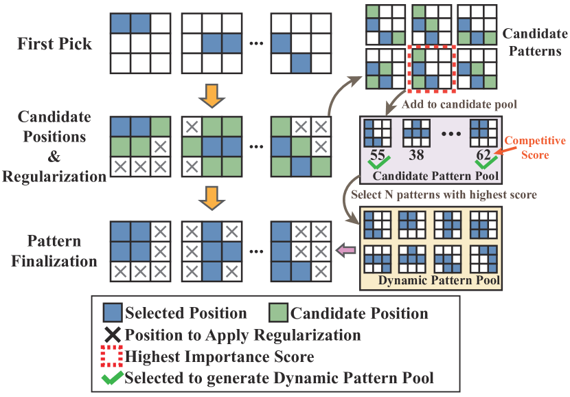
Figure 6. Our proposed DPPG method.

Proposed dynamic pool generation process. The whole process mainly consists of the following six steps. We first select one weight position with the highest estimated importance score in each kernel. We then select the second weight position with the highest importance score among the adjacent positions of the first position, including its horizontal, vertical, and diagonal adjacent position. After determining the first two positions in patterns (marked in blue in Figure 6), we mark the adjacent positions to the first two positions as the “candidate positions” (marked in green). For each kernel, we pick two candidate positions together with the first two positions to form a candidate pattern. We evaluate the importance score (as mentioned in Section 4.1) of all possible combinations (i.e., candidate patterns) to find the candidate pattern with the highest score, then add it to a global candidate pattern pool. Each candidate pattern in the candidate pattern pool has a competitive score that is initialized to 1. If the candidate pattern already exists in the candidate pattern pool, then we add “1” to its competitive score. We repeat the step 1$\sim$4 for a certain number of epochs (depending on the training epoch budget), and keep accumulating the competitive scores in the candidate pattern pool. Finally, we obtain the desired final pattern pool by selecting $N$ candidate patterns from candidate pattern pool with the highest competitive scores, where $N$ is the given number of total pattern types (usually is set to 8 or 12).

Detailed optimizations. In order to better cluster the candidate patterns in the candidate pattern pool and generate a desired pattern pool, we apply several optimizations/constraints during the dynamic pattern pool generation process.

For , the selection rule of the second weight position is derived by considering two observations: i) the position of the most important weight (i.e., the highest-scoring weight) in each kernel is relatively stable after certain training iterations, and ii) the weight distribution in unpruned (dense) well-trained models suggest that the important weights tend to be adjacent to each other.

For , since the weights on the candidate positions are usually less important than the firstly selected two weights, model has a higher tolerance for these weights not being selected optimally. Thus, we intentionally exclude the diagonal adjacent positions to reduce the diversity of the candidate positions to cluster the candidate patterns. Moreover, by limiting the possible candidate positions in , part of the pruning positions (marked as “$\times$” in Figure 6) in each kernel can be determined earlier, thereby starting the regularization and fine tuning sooner, which both reduces the training time and enhances the pattern formation process.

4.3. Adaptive Pattern and Kernel Finalization

After the pattern pool is generated, we can finalize the pattern for each kernel adaptively based on the pattern pool. Due to the concern that the one-time selection method may not provide high accuracy, we propose an adaptive method to finalize the patterns using multiple training epochs. Specifically, in each training batch, for every kernel, we calculate the importance score of each pattern in our pattern pool. Then, we find the pattern with the highest importance score and count its number of occurrences during training. After a number of epochs, the final pattern for each kernel will be selected as the most frequent one of those highest-scoring patterns.

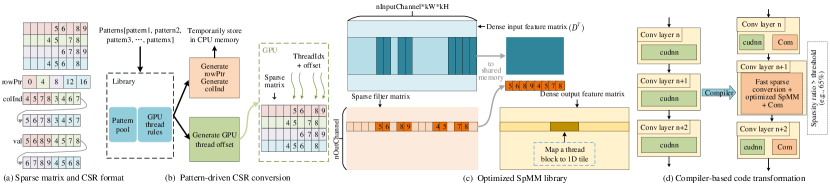
Figure 7. Our proposed compiler-assisted pattern-accelerated SpMM for sparse convolution.

Figure 8. Accuracy comparison between 8 and 12 dynamic patterns.

Similarly, we also use our importance estimation method to calculate the importance score for each kernel and adaptively select a user-set number of unimportant kernels for each layer. Note that the loss is not always decreasing during training. Thus, we set up a training loss margin $\delta$ as a hyperparameter to avoid selecting patterns in the training batches where the loss is obviously increasing. For example, if the loss in the previous batch divided by the value in the current batch is smaller than $0.0018$ (default $\delta$), we will not count the highest-scoring patterns into the number of occurrences. In addition, Figure 8 illustrates that 12 dynamic patterns achieves $2\%$ higher than the one-time solution on CIFAR-10 since kernels have greater probability of selecting the appropriate pattern.

4.4. Modified Group Lasso Regularization

$\ell_{1}$-based regularization or group-lasso regularization is usually added to the loss function to penalize all important or unimportant weights along desired dimensions (such as filter, channel) over the entire layers of CNNs. However, we have noted that using group-lasso regularization to penalize all the weights of filters or channels can lead to a severely impaired pruned model. Thus, we propose a modified group-lasso regularization to more accurately penalize the weights. Generally speaking, unimportant weights should be punished more heavily than important weights, and important weights should remain the same because they typically play a key role in generating stronger activation to make more confident decisions. In particular, after selecting the best-fit pattern for each kernel and identifying the unimportant kernels, we only penalize the unimportant kernels and the weights outside of the selected patterns, since we desire to reduce the absolute values of these weights and kernels as the training progresses. We note that the contributions of these weights/kernels to the final accuracy are negligible, so even if we directly remove (i.e., hard prune) these weights/kernels, the model accuracy would not decrease obviously.

Let $I^{(\ell)}$ be a 4-D importance tensor (i.e., a tensor full of importance scores) of a 4-D weight tensor $W^{(\ell)}$, where $I^{(\ell)}$ is the same shape as $W^{(\ell)}$. Assume the $c_{\ell}$-th kernel of the $f_{\ell}$-th filter in the convolutional layer $\ell$ is unimportant, we set $I^{(\ell)}_{\smash{f_{\ell},\ c_{\ell},:,:}}$ to be 0. Our proposed approach for penalizing unimportant weights and kernels with modified group-lasso regularization can be formulated as:

(3) $$Z^{(\ell)}=W^{(\ell)}\odot\left(\neg P^{(\ell)}\right),\;\;U^{(\ell)}=W^{(\ell)}\odot\left(\neg I^{\hskip 1.04996pt(\ell)}\right)$$

(4) $$\begin{split}\scriptstyle E(W,D)\scriptstyle&=E(W,D)+\lambda_{P}\sum_{l=1}^{L}\left(\sum_{f_{l}=1}^{F_{l}}\sum_{k_{l}=1}^{K_{l}}\left\|Z^{(l)}_{f_{l},k_{l},:,:}\right\|_{g}\right)\scriptstyle\\ &+\lambda_{\mathclap{\ \ I}\phantom{P}}\sum_{l=1}^{L}\left(\sum_{f_{l}=1}^{F_{l}}\sum_{k_{l}=1}^{K_{l}}\left\|U^{(l)}_{f_{l},k_{l},:,:}\right\|_{g}\right)\end{split}$$

where $\scriptstyle\left\|w^{(g)}\right\|_{g}$ = $\scriptstyle\sqrt{\sum_{i=1}^{|w^{(g)}|}\left(w_{i}^{(g)}\right)^{2}}$, $|w^{(g)}|$ is the number of weights in $w^{(g)}$, $\neg$ is the element-wise inversion operator (i.e., 0 $\rightarrow$ 1 or 1 $\rightarrow$ 0), and $\lambda$ is the coefficients for the group-lasso regularization. Here the inverse tensors $\neg P^{(\ell)}$ and $\neg I^{(\ell)}$ can be considered as masks, which can prevent from unnecessarily penalizing the important weights. Moreover, these tensor operations can be accelerated by many popular GPU-based deep learning frameworks such as TensorFlow and PyTorch (Abadi et al., 2016; Paszke et al., 2019) to speedup the group lasso.

5. System-Level Optimizations of ClickTrain

In this section, we discuss our proposed system-level optimizations (used in stage 5) for improving training computation efficiency.

5.1. Pattern-driven Fast Sparse Matrix Conversion

Kernels become much more sparse than origins after pruning. According to prior studies (Choy et al., 2019; Yao et al., 2019), a highly optimized sparse matrix-matrix multiplication (SpMM) leveraging pruning sparsity can outperform state-of-the-art GPU GEMM libraries such as cuBLAS (Nvidia, 2008) for convolution computation. SpMM typically requires converting dense input matrix to a sparse format such as Compressed Sparse Row (CSR) because CSR dominates a continuous storage space, which is beneficial to data locality and computation efficiency.

However, converting a dense matrix to its CSR format (as shown in Figure 7 (a)) usually introduces an obvious time overhead if directly calling dense2csr() from cuSPARSE library (Naumov et al., 2010). For example, as shown in Figure 9, dense2csr() costs about 200 us when converting a 256$\times$1152 dense matrix to its CSR format (generated by the convolution operation on 128$\times$224$\times$224 and 256$\times$128$\times$3$\times$3 tensors), whereas the time of the corresponding SpMM of 256$\times$1152 (sparse) multiplying 1152$\times$50176 (dense) is only about 3000 us. We note that after the patterns have been finalized, the positions of un-pruned (non-zero) weights will not change. Thus, we can directly generate rowPtr, colInd, and GPU thread offset arrays (as shown in Figure 7 (b)) during stage 3 (as shown in Figure 4) and store them for the following SpMM-based convolution operations. Note that this indices generation only introduces a negligible time overhead, since we only need to generate the fixed arrays for once and keep using them in the next stages.

Figure 9. CSR conversion time.

Moreover, since dense2csr() does not provide any interface for pre-defined nonzero positions (rowPtr and colInd), we propose a fast dense-to-sparse matrix conversion routine with pre-defined nonzero positions, whose interface as follow.

template <typename T> Convert2CSR(int* rowPtr, int* colInd, T* sparseFilters, T* val)

Note that in order to maintain a minimal modification to the existing popular deep learning frameworks such as PyTorch which uses dense matrices for most computations such as autograd (automatic differentiation), we apply our fast dense-to-sparse matrix conversion before each SpMM (for all filters in one layer) rather than changing all computations to be based on sparse matrices.

For demonstration purpose, we evaluate our proposed fast matrix conversion on the 256$\times$1152 and 1152$\times$50176 matrices using an NVIDIA RTX 5000 GPU and compare it with cuSPARSE. Figure 9 illustrates that our conversion implementation is 4$\times$ faster than cuSPARSE’s dense2csr().

5.2. Pattern-Accelerated SpMM for Sparse Convolution

Ideally, we can save the floating-point operations if not involving the pruned weights (zeros) in the convolution operation. However, even though pattern sparsity is more regular than random sparsity (unstructured pruning), existing hardware such as GPUs cannot utilize the pattern sparsity to accelerate either forward or backward phase. We observe that our pattern sparsity exhibits three key characteristics: The types of sparsity is relatively limited, such as 4, 8, or 12. The non-zero (un-pruned) weights inside a kernel are more likely close to each other. Each kernel has the same number of non-zero weights. Therefore, considering that SpMM can decrease the computational cost for sparse convolution operations by reducing the number of multiplications and additions, we propose to design a new GPU SpMM library for sparse convolution to make full use of the above important characteristics and use CUDAAdvisor (Shen et al., 2018) to guide CUDA code optimization.

Pattern-Accelerated SpMM. We first describe our design of pattern-accelerated GPU SpMM library that exploits the pattern sparsity in both forward and backward phases. Specifically, converted sparse matrices after pruning lose the regular structure of dense matrices, which results in irregular memory accesses in SpMM. Moreover, concurrently executing massive threads on GPU makes the random memory access issue worse. Thus, improper handling of random memory accesses from massive parallel threads would stall the thread execution and decrease the performance significantly. In order to overcome the challenge of random memory accesses, we propose to take advantage of shared memory on GPU architectures to support concurrent random accesses. Specifically, we first load a tile of data from input feature matrix (dense) and filter matrix (sparse) to shared memory, as shown in Figure 7 (c). Then, we use the loaded data (in shared memory) to calculate the corresponding tile of output feature matrix (dense). Inspired by existing works (Huang et al., 2020; Gale et al., 2020), load imbalance may severely hurt the performance on the GPU, while we solve this issue through an algorithm-hardware co-design. On the algorithm side, we limit all the filters in the same layer have the same number of un-pruned (non-zero) weights in our pattern-based pruning. On the hardware side, we can further improve the performance by using the vectorized load and store instructions in CUDA architectures (Luitjens, 2013) because each row of sparse filter matrix has the same length (i.e., non-zero weights). In addition, since the sparse matrices generated by convolution operations typically have relative long rows, we adopt 1D tiling strategy and map each thread block to a 1D

Figure 10. Convolution time with different methods.

For demonstration purpose, we also evaluate our optimized SpMM on those 256$\times$1152 and 1152$\times$50176 matrices using an NVIDIA RTX 5000 GPU and compare it with state-of-the-art dense or sparse GEMM libraries. Figure 10 illustrates that our optimized SpMM library can achieve a speedup of 4.5$\times$ over cuSPARSE. Moreover, our implementation is faster than cuBLAS’s GEMM and cuDNN’s convolution when the sparsity ratio is higher than 65%.

Forward Phase Acceleration. To achieve a final high accuracy, the filters in different layers may have completely different compression/sparsity ratio. We note that for relatively low sparsity ratio, our optimized SpMM does not gain a performance improvement compared to its dense counterpart (will be showed later). Thus, we set a threshold of sparsity ratio for each layer, and only call our optimized SpMM for the layer where its sparsity ratio is higher than the threshold in the forward phase. Based on experiment, we set 65% as the default threshold for all layers without loss of generality.

Backward Phase Acceleration. The output $z^{\ell}$ (before activate function $\sigma$) of the convolutional layer $\ell$ in the CNNs’ forward-propagation is obtained by $z^{\ell}=a^{\ell-1}\circledast W^{\ell}+b^{\ell}$, where $a^{\ell-1}$ is the activations at layer $\ell-1$, $W^{\ell}$ and $b^{\ell}$ denote weights and biases at layer $\ell$, respectively, and $\circledast$ is the convolution operation. In backpropagation, the layer $\ell$ first receives $\delta^{\ell}$ from the layer $\ell+1$, and then $\delta^{\ell}$ is propagated back based on $\delta^{\ell}={\textstyle\frac{\partial E(W,D)}{\partial z^{\ell}}},\delta^{\ell-1}=\delta^{\ell}\circledast\text{rot180}(W^{\ell})\odot\sigma^{\prime}(z^{\ell-1}).$ We can calculate the gradient of the layer $\ell$ after obtaining $\delta^{\ell}$ and $\frac{\partial E(W,D)}{\partial W^{\ell}}=a^{\ell-1}\circledast\delta^{\ell}$. We can observe from the above equation that the difference between forward and backward phases is that the forward phase uses feature map $a^{\ell-1}$ as input, whereas the backward phase uses $\delta^{\ell+1}$ as input. Also, the sparse weight matrix $W^{\ell}$ is involved in the backpropagation, so we adopt the similar strategy as forward phase to handle $W^{\ell}$.

5.3. Communication Optimization

Distributed training has been widely used for larges-scale DNN training. However, gradients must be synchronized among different computing nodes for each training batch, such communication (i.e., Allreduce) overhead is not negligible and will be scaled up as the number of computing nodes increases. Note that since all the weights to be pruned remain zeros after the regularized training stage, we do not need to send the corresponding gradients to other computing nodes in the rest of the training process. Moreover, high sparsity ratio of our pattern-based pruning provides a great opportunity to significantly reduce the communication overhead.

5.4. Compiler-Assisted Optimized Code Generation

After implementing our optimized libraries for sparse matrix conversion, SpMM, and Allreduce, we proposes a compiler-assisted method to generate the optimized code for efficient training (in stage 5). Specifically, after sparsity ratios have been determined (after stage 3), the compiler decides whether using original sparse convolutions or our optimized SpMM computation for each layer in the computational graph based on its sparsity ratio; and accordingly generates the code with the better operator in the training framework such as PyTorch (as shown in Figure 7 (d)). Moreover, the compiler transforms all Allreduce communications (in stage 5) in the computational graph into our optimized pattern-based communications. Note that there is an alternative solution that relies on compiler to generate the shared library calling sparse convolutions or SpMM computation dynamically for each layer. However, this solution introduces “if-else” overhead for each layer in every training batch, which is much higher than the former solution.

6. Experimental Evaluation

In this section, we first evaluate our proposed ClickTrain on different CNNs and datasets and show its accuracy and compression ratio and compare it with several state-of-the-art PDT-/PAT-based frameworks. We then evaluate our proposed optimizations and overall training efficiency on a single GPU and multiple GPUs.

6.1. Experimental Setup

We conduct our experimental evaluation using the Frontera supercomputer (Stanzione et al., 2020) at TACC, of which each GPU node is equipped with two Intel E5-2620 v4 CPUs and four NVIDIA Quadro RTX 5000 GPUs (5000, 2020), interconnected by FDR InfiniBand. We use NVIDIA CUDA 10.1 and its default profiler for time measurement. We implement ClickTrain based on PyTorch (Paszke et al., 2019) using SGD. We evaluate ClickTrain and compare it with state-of-the-art methods on seven well-known CNNs including ResNet18/32/50/101 and VGG11/13/16. Our datasets include CIFAR10/100 (CIFAR-10 and CIFAR-100, 2020) and ImageNet-2012 (Large Scale Visual Recognition Challenge, 2020). Note that all accuracy shown in the following evaluation are based on the average of 10 experiments (variance lower than 0.2%).

Regarding hyperparamter, we initialize the learning rate as 0.1 and set the regularization penalty coefficient as 0.00025. The threshold in stage 1 used for determining when to start stage 2 is set to 0.027. The number of candidate patterns in stage 3 is set to 12, as suggested by Figure 8. We use the bath size (per GPU) of 128 and 64 for CIFAR and ImageNet, respectively.

6.2. Model Accuracy and Ratio Evaluation

Table 1. Comparison between ClickTrain (CLK) and PDT-based method PruneTrain (PRT). FLOPs are the saved FLOPs.

We first evaluate our proposed ClickTrain on different CNNs and datasets with a fixed number of training epochs, as shown in Table 1. We use $\Delta$ to denote the validation accuracy drop of the pruned model compared to the original baseline model. Note that at the end of the regularized training stage, we conduct a hard-pruning step (as shown in Figure 4) to eventually zero out the pruned weights which have been regularized to tiny values. Thus, the rest of training process can be accelerated through our compiler-assisted training optimizations. We train the baseline models to a high accuracy using 190 epochs and 90 epochs for CIFAR10/100 and ImageNet, respectively. It is worth noting that all the above baseline accuracies have been widely used in many previous studies (Lym et al., 2019; Niu et al., 2020b; Ma et al., 2020b). We thus use the same 190 epochs and 90 epochs for ClickTrain on CIFAR and ImageNet, respectively. We calculate the compression ratio only considering the convolutional layers in the models, since the convolutional layers in ResNet and VGG models dominate most of the computation overhead in both training and inference processes. In particular, the compression ratio is calculated as $\frac{\text{the total number of weights}}{\text{the total number of nonzero weights}}$ based on all the convolutional layers.

Table 1 illustrates that for ResNet32 and ResNet50, our ClickTrain can provide more than 10$\times$ compression ratio while maintaining up to 0.2% accuracy drop on the two CIFAR datasets, compared to the baseline accuracy. For VGG11/13, ClickTrain can also provide 8.6$\times$ to 11.5$\times$ compression ratio with up to 0.3% accuracy drop. Since most of the weights in the convolutional layers have been pruned, ClickTrain can save the training FLOPs and inference FLOPs by 36.7%$\sim$45.2% and 73.6%$\sim$85.7%, respectively, on CIFAR10/100 with the assist of compiler optimizations. To demonstrate the effectiveness on large dataset, we also train ResNet50 on ImageNet using ClickTrain. It provides a compression ratio of 4.3$\times$ and saves the training/inference FLOPs by 36.9%/66%.

Note that the higher the compression ratio, the faster the inference of pruned model. For example, previous studies (Niu et al., 2020b; Rumi et al., 2020) proved that for ResNet50 on ImageNet, a compression ratio of about 4.3 (as same as ClickTrain’s) with the pattern-based pruning (adopted by ClickTrain) reduces the model inference latency (batch size 1) by 11$\times$ on the Qualcomm Snapdragon 855 mobile platform (with a Qualcomm Kryo 485 octa-core CPU); in comparison, a previous work (Wang et al., 2020) illustrates that a compression ratio of about 2.1 (as same as Prunetrian’s) with the structure pruning (adopted by Prunetrian) reduces the inference latency by only 0.72$\times$ on an Intel Xeon E5-2680 v4 CPU. Note that the single-core performance difference between Kryo 485 and Xeon E5-2680 v4 is within 5% (ntel Xeon E5-2680 v4 vs Qualcomm SM8150 Snapdragon 855, 2020).

Table 2. Comparison between ClickTrain and PAT-based methods on ImageNet. Well-train costs about 90 epochs.

PAT Method Base. Acc. Valid. Acc. $\Delta$ Comp. Ratio Total Epochs ResNet-18 TAS (Dong and Yang, 2019) 70.6% $-$1.5% 1.5$\times$ 120 DCP (Zhuang et al., 2018) 69.6% $-$5.5% 3.3$\times$ well train + 60 CLK 69.6% $-$0.9% 4.1$\times$ 90 ResNet-50 GBN (You et al., 2019b) 75.8% $-$0.6% 2.2$\times$ well train + 60 GAL (Lin et al., 2019) 76.4% $-$7.1% 2.5$\times$ well train + 30 CLK 76.1% $-$0.7% 4.3$\times$ 90 ResNet-101 RSNLIA (Ye et al., 2018) 75.27% $-$2.1% 1.9$\times$ well train + tune CLK 76.4% $-$1.2% 4.2$\times$ 90 VGG-16 NeST (Dai et al., 2019) 71.6% $-$2.3% 6.5$\times$ N/A CLK 73.1% $-$0.8% 6.6$\times$ 90

We also evaluate the impact of when to start the hard pruning on the validation accuracy and FLOPs. We observe that the earlier the patterns and unimportant kernels are determined, the earlier the models can be hard pruned by ClickTrain, thus more training FLOPs can be saved; however, earlier hard pruning causes a significant accuracy loss. The epoch of hard pruning shown in Table 1 makes a good tradeoff between accuracy and training FLOPs.

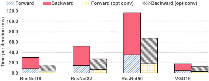
(a) CIFAR

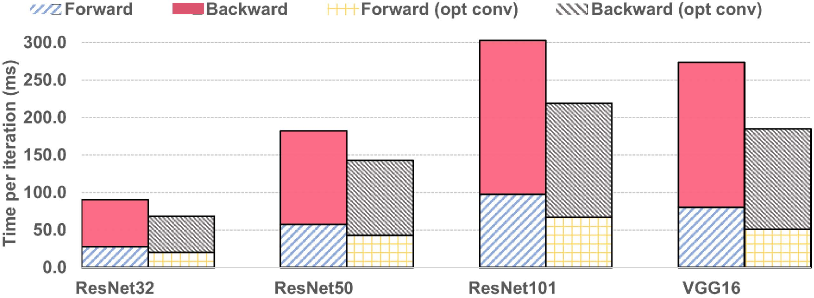
(b) ImageNet

Figure 11. Average forward and backward time per iteration on CIFAR and ImageNet using a single GPU. “opt conv” means solution with our optimized SpMM for sparse convolution.

Comparison with PDT-based Method. We then compare our ClickTrain with the state-of-the-art PDT-based method PruneTrain, as shown in Table 1. It illustrates that ClickTrain can precisely control the accuracy drop within -0.3% for all the tested models on CIFAR10/100, but the accuracy drop of PruneTrain is over -1.0% for most of the tested CNN models. Moreover, ClickTrain can significantly improve the compression ratio with similar or even higher accuracy, compared to PruneTrain. For example, PruneTrain can only provide a compression ratio less than 3$\times$ with more than 1.0% accuracy drop for ResNet50 on CIFAR10, whereas ClickTrain achieves 10.8$\times$ compression ratio with only 0.2% accuracy drop, leading to 4.7$\times$ higher compression ratio. For VGG13 on CIFAR100, ClickTrain achieves 9.2$\times$ compression ratio with only 0.2% accuracy drop, which significantly outperforms PruneTrain’s 2.9$\times$ compression ratio with 1.1% accuracy drop. For ImageNet, ClickTrain reduces the accuracy drop by 1.3% and improves the compression ratio by 2.1$\times$ over PruneTrain.

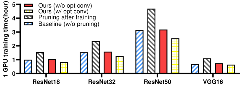
(a) CIFAR10

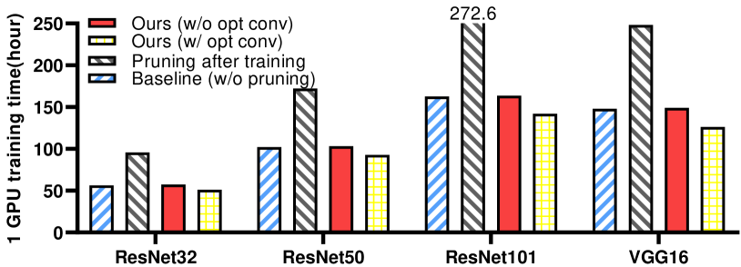
(b) ImageNet

Figure 12. Total training time on CIFAR and ImageNet (single-GPU).

Comparison with PAT-based Methods. A typical procedure of model pruning is removing the redundant weights based on well-trained networks and then fine tuning the slashed networks. Thus, we finally compare our ClickTrain with state-of-the-art PAT-based methods. As illustrated in Table 2, ClickTrain save up to about 67% computation time while only sacrificing up to 1.2% accuracy, compared with other PAT-based methods. In addition, ClickTrain also achieves a much higher compression ratio for efficient inference. Thus, we conclude that accurately estimating the weight importance during training makes our PDT-based solution feasible to significantly save the total training epochs.

6.3. Single-GPU Performance Evaluation

Then, we evaluate the single-GPU performance gain by our PDT-based algorithm and optimized SpMM of ClickTrain.

Forward and Backward Acceleration. We first evaluate the forward and backward time per iteration on a single GPU when applying our optimized SpMM using different CNN models with CIFAR and ImageNet. The sparsity (i.e., compression ratio) for each model can be found in Table 2.

Figure 11(a) shows that for forward phase on CIFAR, ClickTrain achieves the speedups of 2.2$\times$, 2.1$\times$, and 1.9$\times$, and 1.6$\times$ on ResNet18, ResNet32, ResNet50, and VGG16, respectively. For backward phase, ClickTrain achieves the speedups of 1.8$\times$, 1.7$\times$, 1.6$\times$, and 1.3$\times$ on ResNet18, ResNet32, ResNet50, and VGG16, respectively. Figure 11(b) shows that for forward phase on ImageNet, ClickTrain achieves the speedups of 1.4$\times$, 1.3$\times$, 1.5$\times$, and 1.6$\times$ on ResNet32, ResNet50, ResNet101, and VGG16, respectively. For backward phase on imagenet, ClickTrain achieves the speedups of 1.3$\times$, 1.25$\times$, 1.35$\times$, and 1.5$\times$ on ResNet32, ResNet50, ResNet101, and VGG16, respectively.

Overall Training Acceleration. We then evaluate the training acceleration of ClickTrain with the four CNNs on CIFAR10 and ImageNet, as shown in Figure 12(a). Compared with the baseline training (i.e., training without pruning), ClickTrain saves 0.16, 0.29, 0.59, and 0.15 hours on ResNet18/32/50 and VGG16, respectively, on CIFAR10. When training on ImageNet, ClickTrain saves 5.1, 9.4, 20.4, and 19.7 hours on ResNet32/50/101 and VGG16, respectively.

6.4. Multi-GPU Performance Evaluation

Communication Time. Next, we evaluate our optimized communication time using multiple GPUs on ResNet50, ResNet101 and VGG16 with ImageNet, as shown in Figure 13. For ResNet50, ClickTrain can save 23.9%, 26.3%, and 28.4% communication time per iteration using 4, 8, and 16 GPUs, respectively. For ResNet101, ClickTrain can save 27.5%, 29.7%, and 31.2% communication time per iteration using 4, 8, and 16 GPUs, respectively. For VGG16, ClickTrain can save 21.2%, 24.3%, and 24.9% communication time per iteration using 4, 8, and 16 GPUs, respectively. We notice that although PyTorch’s optimization of communication and computation overlap offsets our optimization for communication overhead to some extent, the performance gain will increase when increasing the scale (i.e., number of nodes and GPUs).

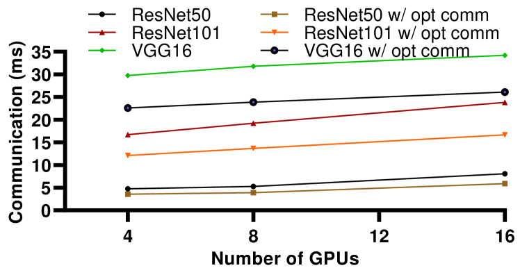
Figure 13. Communication time of baseline training and ClickTrain with different numbers of GPUs. “opt comm” means solution with our optimized communication.

Total Training Time. Furthermore, we evaluate the overall training time on different CNN models using ImageNet with batch size 64 per GPU. Figure 14 shows that compared with the baseline training, for on ResNet50, ClickTrain saves 3.2 hours, 2.1 hours, and 1.4 hours using 4, 8, and 16 GPUs, respectively; for ResNet101, ClickTrain saves 7.1 hours, 4 hours, and 2.5 hours using 4, 8, and 16 GPUs, respectively; for on VGG16, ClickTrain saves 6.3 hours, 4.6 hours, and 2.7 hours using 4, 8, and 16 GPUs, respectively. Note that unlike the baseline training, ClickTrain can generate ready-to-deploy models without further tuning such as pruning. Moreover, compared with the baseline PAT-based approach (i.e., pattern-based pruning after training), ClickTrain reduces the training time by 1.67$\times$/1.96$\times$/2.13$\times$, 1.86$\times$/1.99$\times$/2.18$\times$, and 1.98$\times$/2.15$\times$/2.25$\times$ using 4, 8, and 16 GPUs, respectively, on ResNet50/ResNet101/VGG16.

Comparison with PruneTrain. Finally, Figure 15a shows that ClickTrain achieves a compression ratio of 10.8$\times$ with only 0.2% accuracy drop on ResNet50 with CIFAR10, whereas PruneTrain only has 2.3$\times$ compression ratio but with a significant accuracy drop of 1.1%, even it saves 16.7% end-to-end time over ClickTrain. Figure 15b shows that ClickTrain has 2.1$\times$ higher compression ratio than PruneTrain with a notable accuracy improvement of 1.3% on ResNet50 with ImageNet but only slightly longer (i.e., 18.4%) end-to-end time. Note that 1.3% on ImageNet and 0.9% on CIFAR10 are significant accuracy improvements considering the limited training time. Thus, aggressively preserving the original architecture is critical for designing PDT-based approaches.

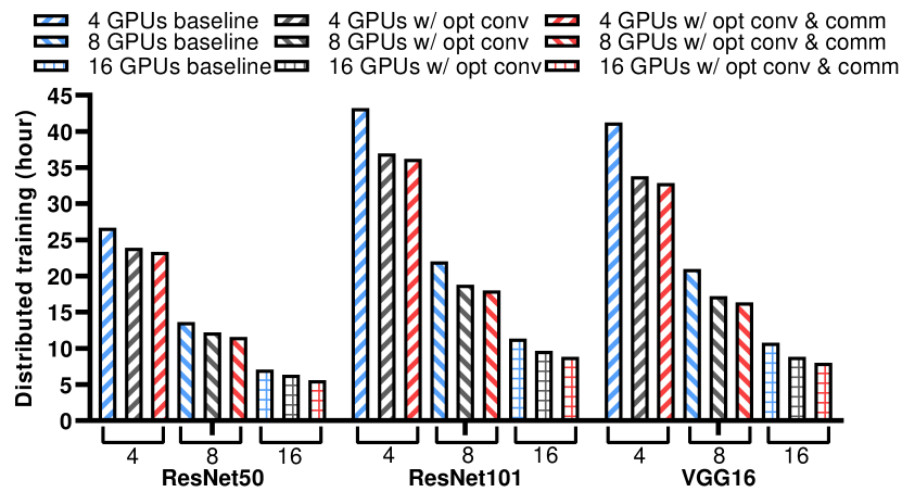
Figure 14. Total time of baseline training and ClickTrain.

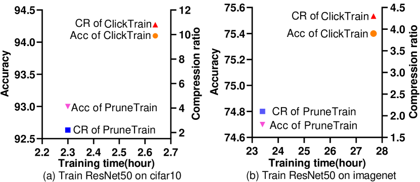
Figure 15. Comparison of PruneTrain and ClickTrain.

7. Related Work

PruneTrain (Lym et al., 2019) is a state-of-the-art approach to accelerate the DNN training from scratch while pruning it. The work observed that when pruning with group-lasso regularization, once a group of model weights are penalized close to zero, their magnitudes are typically impossible to recover during the rest of the training process. Based on this observation, PruneTrain periodically removes the small weights and reconfigure the network architecture and hence can gradually reduce the training during training toward both high compression ratio and accuracy. In addition, PruneTrain also proposes to dynamically increase the mini-batch to further increase the training performance. However, as we discussed in Section 3, PruneTrain aggressively change the original network architecture, causing a significant unrecoverable accuracy loss.

The lottery ticket hypothesis (Frankle and Carbin, 2018) proves that subnetworks can match the test accuracy of original network after training for at most the same number of iterations. Those subnetworks are termed as winning tickets, which can be directly trained efficiently. However, it is challenging to determine the architecture of subnetwork.

The Early-Bird (EB) tickets work (You et al., 2019a) claims that winning tickets can be identified at a very early training stage using aggressively low-cost training algorithms. Even though EB also adopts the strategy that firstly trains a few epochs and then prunes the network, it chooses channel pruning, which will change the network architecture and lead to a significant accuracy drop.

8. Conclusion

In this paper, we propose ClickTrain by using dynamic fine-grained pattern-based pruning. It has both algorithm-level and system-level optimizations with four stages. i) accurate weight importance estimation to select the pattern, ii) dynamic pattern generation and finalization, iii) regularized training for fine-tuning with an enhanced group-lasso, and iv) compiler-assisted optimized training. Our experimental results on seven DNNs and three datasets demonstrate that ClickTrain can reduce the cost of the state-of-the-art PAT-based method by up to 2.3$\times$ with comparable accuracy and compression ratio. Compared with the state-of-the-art training acceleration approach, ClickTrain can improve the pruned accuracy by up to 1.8% and the compression ratio by up to 4.9$\times$ on the tested CNNs and datasets, with comparable training time. We plan to extend ClickTrain to more types of DNNs in the future.

References

- (1)
- 5000 (2020) NVIDIA QUADRO RTX 5000. 2020. https://www.nvidia.com/en-us/design-visualization/quadro/rtx-5000/. Online.
- Abadi et al. (2016) Martín Abadi, Paul Barham, Jianmin Chen, Zhifeng Chen, Andy Davis, Jeffrey Dean, Matthieu Devin, Sanjay Ghemawat, Geoffrey Irving, Michael Isard, Manjunath Kudlur, Josh Levenberg, Rajat Monga, Sherry Moore, Derek Gordon Murray, Benoit Steiner, Paul A. Tucker, Vijay Vasudevan, Pete Warden, Martin Wicke, Yuan Yu, and Xiaoqiang Zheng. 2016. TensorFlow: A System for Large-Scale Machine Learning. In 12th USENIX Symposium on Operating Systems Design and Implementation (OSDI 16). 265–283.
- Brown et al. (2020) Tom B. Brown, Benjamin Mann, Nick Ryder, Melanie Subbiah, Jared Kaplan, Prafulla Dhariwal, Arvind Neelakantan, Pranav Shyam, Girish Sastry, Amanda Askell, Sandhini Agarwal, Ariel Herbert-Voss, Gretchen Krueger, Tom Henighan, Rewon Child, Aditya Ramesh, Daniel M. Ziegler, Jeffrey Wu, Clemens Winter, Christopher Hesse, Mark Chen, Eric Sigler, Mateusz Litwin, Scott Gray, Benjamin Chess, Jack Clark, Christopher Berner, Sam McCandlish, Alec Radford, Ilya Sutskever, and Dario Amodei. 2020. Language models are few-shot learners. arXiv preprint arXiv:2005.14165 (2020).
- Cai et al. (2020) Yuxuan Cai, Hongjia Li, Geng Yuan, Wei Niu, Yanyu Li, Xulong Tang, Bin Ren, and Yanzhi Wang. 2020. YOLObile: Real-Time Object Detection on Mobile Devices via Compression-Compilation Co-Design. arXiv preprint arXiv:2009.05697 (2020).
- Choy et al. (2019) Christopher Choy, JunYoung Gwak, and Silvio Savarese. 2019. 4d spatio-temporal convnets: Minkowski convolutional neural networks. In Proceedings of the IEEE Conference on Computer Vision and Pattern Recognition. 3075–3084.
- CIFAR-10 and CIFAR-100 (2020) CIFAR-10 and CIFAR-100. 2020. https://www.cs.toronto.edu/~kriz/cifar.html. Online.
- Collobert and Weston (2008) Ronan Collobert and Jason Weston. 2008. A unified architecture for natural language processing: Deep neural networks with multitask learning. In Proceedings of the 25th International Conference on Machine Learning. ACM, 160–167.
- Dai et al. (2019) Xiaoliang Dai, Hongxu Yin, and Niraj K Jha. 2019. NeST: A neural network synthesis tool based on a grow-and-prune paradigm. IEEE Trans. Comput. 68, 10 (2019), 1487–1497.
- Ding et al. (2017) Caiwen Ding, Siyu Liao, Yanzhi Wang, Zhe Li, Ning Liu, Youwei Zhuo, Chao Wang, Xuehai Qian, Yu Bai, Geng Yuan, et al. 2017. Circnn: accelerating and compressing deep neural networks using block-circulant weight matrices. In Proceedings of the 50th Annual IEEE/ACM International Symposium on Microarchitecture. 395–408.
- Ding et al. (2018) Caiwen Ding, Ao Ren, Geng Yuan, Xiaolong Ma, Jiayu Li, Ning Liu, Bo Yuan, and Yanzhi Wang. 2018. Structured weight matrices-based hardware accelerators in deep neural networks: Fpgas and asics. In Proceedings of the 2018 on Great Lakes Symposium on VLSI. 353–358.
- Dong et al. (2020) Peiyan Dong, Siyue Wang, Wei Niu, Chengming Zhang, Sheng Lin, Zhengang Li, Yifan Gong, Bin Ren, Xue Lin, Yanzhi Wang, and Dingwen Tao. 2020. RTMobile: Beyond Real-Time Mobile Acceleration of RNNs for Speech Recognition. arXiv preprint arXiv:2002.11474 (2020).
- Dong and Yang (2019) Xuanyi Dong and Yi Yang. 2019. Network pruning via transformable architecture search. In Advances in Neural Information Processing Systems. 759–770.
- Elsken et al. (2018) Thomas Elsken, Jan Hendrik Metzen, and Frank Hutter. 2018. Neural architecture search: A survey. arXiv preprint arXiv:1808.05377 (2018).
- Frankle and Carbin (2018) Jonathan Frankle and Michael Carbin. 2018. The lottery ticket hypothesis: Finding sparse, trainable neural networks. arXiv preprint arXiv:1803.03635 (2018).
- Freeman and Adelson (1991) W. T. Freeman and E. H. Adelson. 1991. The design and use of steerable filters. IEEE Transactions on Pattern Analysis and Machine Intelligence 13, 9 (1991), 891–906.
- Gale et al. (2020) Trevor Gale, Matei Zaharia, Cliff Young, and Erich Elsen. 2020. Sparse GPU Kernels for Deep Learning. arXiv preprint arXiv:2006.10901 (2020).
- Geng et al. (2019) Tong Geng, Tianqi Wang, Chunshu Wu, Chen Yang, Shuaiwen Leon Song, Ang Li, and Martin Herbordt. 2019. LP-BNN: Ultra-low-latency BNN inference with layer parallelism. In 2019 IEEE 30th International Conference on Application-specific Systems, Architectures and Processors (ASAP), Vol. 2160. IEEE, 9–16.
- Han et al. (2016) Song Han, Xingyu Liu, Huizi Mao, Jing Pu, Ardavan Pedram, Mark Horowitz, and Bill Dally. 2016. Deep compression and EIE: Efficient inference engine on compressed deep neural network.. In Hot Chips Symposium. 1–6.
- He et al. (2016) Kaiming He, Xiangyu Zhang, Shaoqing Ren, and Jian Sun. 2016. Deep residual learning for image recognition. In Proceedings of the IEEE conference on computer vision and pattern recognition. 770–778.
- He et al. (2018) Yang He, Guoliang Kang, Xuanyi Dong, Yanwei Fu, and Yi Yang. 2018. Soft Filter Pruning for Accelerating Deep Convolutional Neural Networks. In Proceedings of the 27th International Joint Conference on Artificial Intelligence. 2234–2240.
- He et al. (2017) Yihui He, Xiangyu Zhang, and Jian Sun. 2017. Channel Pruning for Accelerating Very Deep Neural Networks. In Proceedings of the IEEE International Conference on Computer Vision. IEEE, 1398–1406.
- Huang et al. (2020) Guyue Huang, Guohao Dai, Yu Wang, and Huazhong Yang. 2020. GE-SpMM: General-purpose Sparse Matrix-Matrix Multiplication on GPUs for Graph Neural Networks. arXiv preprint arXiv:2007.03179 (2020).
- Jin et al. (2019) Sian Jin, Sheng Di, Xin Liang, Jiannan Tian, Dingwen Tao, and Franck Cappello. 2019. DeepSZ: A Novel Framework to Compress Deep Neural Networks by Using Error-Bounded Lossy Compression. In Proceedings of the 28th International Symposium on High-Performance Parallel and Distributed Computing. ACM, 159–170.
- Krizhevsky et al. (2012) Alex Krizhevsky, Ilya Sutskever, and Geoffrey E Hinton. 2012. Imagenet classification with deep convolutional neural networks. In Advances in neural information processing systems. 1097–1105.
- Large Scale Visual Recognition Challenge (2020) Large Scale Visual Recognition Challenge. 2020. http://www.image-net.org/challenges/LSVRC/. Online.
- Li et al. (2019) Ang Li, Tong Geng, Tianqi Wang, Martin Herbordt, Shuaiwen Leon Song, and Kevin Barker. 2019. BSTC: A novel binarized-soft-tensor-core design for accelerating bit-based approximated neural nets. In Proceedings of the International Conference for High Performance Computing, Networking, Storage and Analysis. 1–30.
- Li et al. (2021) Hongjia Li, Geng Yuan, Wei Niu, Yuxuan Cai, Mengshu Sun, Zhengang Li, Bin Ren, Xue Lin, and Yanzhi Wang. 2021. Real-Time Mobile Acceleration of DNNs: From Computer Vision to Medical Applications. In 2021 26th Asia and South Pacific Design Automation Conference (ASP-DAC). IEEE, 581–586.
- Li et al. (2020) Zhengang Li, Yifan Gong, Xiaolong Ma, Sijia Liu, Mengshu Sun, Zheng Zhan, Zhenglun Kong, Geng Yuan, and Yanzhi Wang. 2020. SS-Auto: A Single-Shot, Automatic Structured Weight Pruning Framework of DNNs with Ultra-High Efficiency. arXiv preprint arXiv:2001.08839 (2020).
- Lin et al. (2019) Shaohui Lin, Rongrong Ji, Chenqian Yan, Baochang Zhang, Liujuan Cao, Qixiang Ye, Feiyue Huang, and David Doermann. 2019. Towards optimal structured cnn pruning via generative adversarial learning. In Proceedings of the IEEE Conference on Computer Vision and Pattern Recognition. 2790–2799.
- Liu et al. (2018) Zhuang Liu, Mingjie Sun, Tinghui Zhou, Gao Huang, and Trevor Darrell. 2018. Rethinking the value of network pruning. arXiv preprint arXiv:1810.05270 (2018).
- Luitjens (2013) Justin Luitjens. 2013. CUDA Pro Tip: Increase Performance with Vectorized Memory Access. https://developer.nvidia.com/blog/cuda-pro-tip-increase-performance-with-vectorized-memory-access/. Online.
- Luo et al. (2017) Jian-Hao Luo, Jianxin Wu, and Weiyao Lin. 2017. Thinet: A filter level pruning method for deep neural network compression. In Proceedings of the IEEE international conference on computer vision. 5058–5066.
- Lym et al. (2019) Sangkug Lym, Esha Choukse, Siavash Zangeneh, Wei Wen, Sujay Sanghavi, and Mattan Erez. 2019. PruneTrain: fast neural network training by dynamic sparse model reconfiguration. In Proceedings of the International Conference for High Performance Computing, Networking, Storage and Analysis. 1–13.
- Ma et al. (2019a) Xiaolong Ma, Fu-Ming Guo, Wei Niu, Xue Lin, Jian Tang, Kaisheng Ma, Bin Ren, and Yanzhi Wang. 2019a. Pconv: The missing but desirable sparsity in dnn weight pruning for real-time execution on mobile devices. arXiv preprint arXiv:1909.05073 (2019).
- Ma et al. (2020a) Xiaolong Ma, Zhengang Li, Yifan Gong, Tianyun Zhang, Wei Niu, Zheng Zhan, Pu Zhao, Jian Tang, Xue Lin, Bin Ren, and Yanzhi Wang. 2020a. BLK-REW: A Unified Block-based DNN Pruning Framework using Reweighted Regularization Method. arXiv preprint arXiv:2001.08357 (2020).
- Ma et al. (2021) Xiaolong Ma, Sheng Lin, Shaokai Ye, Zhezhi He, Linfeng Zhang, Geng Yuan, Sia Huat Tan, Zhengang Li, Deliang Fan, Xuehai Qian, et al. 2021. Non-Structured DNN Weight Pruning–Is It Beneficial in Any Platform? IEEE Transactions on Neural Networks and Learning Systems (2021).
- Ma et al. (2019b) Xiaolong Ma, Sheng Lin, Shaokai Ye, Zhezhi He, Linfeng Zhang, Geng Yuan, Sia Huat Tan, Zhengang Li, Deliang Fan, Xuehai Qian, Xue Lin, Kaisheng Ma, and Yanzhi Wang. 2019b. Non-Structured DNN Weight Pruning – Is It Beneficial in Any Platform? arXiv:cs.LG/1907.02124
- Ma et al. (2020b) Xiaolong Ma, Wei Niu, Tianyun Zhang, Sijia Liu, Fu-Ming Guo, Sheng Lin, Hongjia Li, Xiang Chen, Jian Tang, Kaisheng Ma, Bin Ren, and Yanzhi Wang. 2020b. An Image Enhancing Pattern-based Sparsity for Real-time Inference on Mobile Devices. arXiv preprint arXiv:2001.07710 (2020).
- Ma et al. (2020c) Xiaolong Ma, Geng Yuan, Sheng Lin, Caiwen Ding, Fuxun Yu, Tao Liu, Wujie Wen, Xiang Chen, and Yanzhi Wang. 2020c. Tiny but accurate: A pruned, quantized and optimized memristor crossbar framework for ultra efficient dnn implementation. In 2020 25th Asia and South Pacific Design Automation Conference (ASP-DAC). IEEE, 301–306.
- Ma et al. (2019c) Xiaolong Ma, Geng Yuan, Sheng Lin, Zhengang Li, Hao Sun, and Yanzhi Wang. 2019c. ResNet Can Be Pruned 60: Introducing Network Purification and Unused Path Removal (P-RM) after Weight Pruning. In 2019 IEEE/ACM International Symposium on Nanoscale Architectures (NANOARCH). IEEE, 1–2.
- Ma et al. (2018) Xiaolong Ma, Yipeng Zhang, Geng Yuan, Ao Ren, Zhe Li, Jie Han, Jingtong Hu, and Yanzhi Wang. 2018. An area and energy efficient design of domain-wall memory-based deep convolutional neural networks using stochastic computing. In 2018 19th International Symposium on Quality Electronic Design (ISQED). IEEE, 314–321.
- Meier et al. (2008) Lukas Meier, Sara Van De Geer, and Peter Bühlmann. 2008. The group lasso for logistic regression. Journal of the Royal Statistical Society: Series B (Statistical Methodology) 70, 1 (2008), 53–71.
- Molchanov et al. (2019) Pavlo Molchanov, Arun Mallya, Stephen Tyree, Iuri Frosio, and Jan Kautz. 2019. Importance estimation for neural network pruning. In Proceedings of the IEEE Conference on Computer Vision and Pattern Recognition. 11264–11272.
- Molchanov et al. (2016) Pavlo Molchanov, Stephen Tyree, Tero Karras, Timo Aila, and Jan Kautz. 2016. Pruning convolutional neural networks for resource efficient inference. arXiv preprint arXiv:1611.06440 (2016).
- Naumov et al. (2010) M Naumov, LS Chien, P Vandermersch, and U Kapasi. 2010. Cusparse library. In GPU Technology Conference.
- Niu et al. (2020a) Wei Niu, Zhenglun Kong, Geng Yuan, Weiwen Jiang, Jiexiong Guan, Caiwen Ding, Pu Zhao, Sijia Liu, Bin Ren, and Yanzhi Wang. 2020a. Achieving Real-Time Execution of Transformer-based Large-scale Models on Mobile with Compiler-aware Neural Architecture Optimization. arXiv preprint arXiv:2009.06823 (2020).
- Niu et al. (2020b) Wei Niu, Xiaolong Ma, Sheng Lin, Shihao Wang, Xuehai Qian, Xue Lin, Yanzhi Wang, and Bin Ren. 2020b. Patdnn: Achieving real-time DNN execution on mobile devices with pattern-based weight pruning. In Proceedings of the Twenty-Fifth International Conference on Architectural Support for Programming Languages and Operating Systems (ASPLOS).
- ntel Xeon E5-2680 v4 vs Qualcomm SM8150 Snapdragon 855 (2020) ntel Xeon E5-2680 v4 vs Qualcomm SM8150 Snapdragon 855. 2020. https://gadgetversus.com/processor/intel-xeon-e5-2680-v4-vs-qualcomm-sm8150-snapdragon-855/. Online.
- Nvidia (2008) CUDA Nvidia. 2008. Cublas library. NVIDIA Corporation, Santa Clara, California 15, 27 (2008), 31.
- Paszke et al. (2019) Adam Paszke, Sam Gross, Francisco Massa, Adam Lerer, James Bradbury, Gregory Chanan, Trevor Killeen, Zeming Lin, Natalia Gimelshein, Luca Antiga, Alban Desmaison, Andreas Köpf, Edward Yang, Zachary DeVito, Martin Raison, Alykhan Tejani, Sasank Chilamkurthy, Benoit Steiner, Lu Fang, Junjie Bai, and Soumith Chintala. 2019. PyTorch: An imperative style, high-performance deep learning library. In Advances in Neural Information Processing Systems. 8024–8035.
- Roy et al. (2018) Probir Roy, Shuaiwen Leon Song, Sriram Krishnamoorthy, Abhinav Vishnu, Dipanjan Sengupta, and Xu Liu. 2018. Numa-caffe: Numa-aware deep learning neural networks. ACM Transactions on Architecture and Code Optimization (TACO) 15, 2 (2018), 1–26.
- Rumi et al. (2020) Masuma Akter Rumi, Xiaolong Ma, Yanzhi Wang, and Peng Jiang. 2020. Accelerating Sparse CNN Inference on GPUs with Performance-Aware Weight Pruning. In Proceedings of the ACM International Conference on Parallel Architectures and Compilation Techniques. 267–278.
- Shen et al. (2018) Du Shen, Shuaiwen Leon Song, Ang Li, and Xu Liu. 2018. Cudaadvisor: Llvm-based runtime profiling for modern gpus. In Proceedings of the 2018 International Symposium on Code Generation and Optimization. 214–227.
- Simonyan and Zisserman (2014) Karen Simonyan and Andrew Zisserman. 2014. Very deep convolutional networks for large-scale image recognition. arXiv preprint arXiv:1409.1556 (2014).
- Stanzione et al. (2020) Dan Stanzione, John West, R Todd Evans, Tommy Minyard, Omar Ghattas, and Dhabaleswar K Panda. 2020. Frontera: The evolution of leadership computing at the national science foundation. In Practice and Experience in Advanced Research Computing. 106–111.
- Szegedy et al. (2015) Christian Szegedy, Wei Liu, Yangqing Jia, Pierre Sermanet, Scott Reed, Dragomir Anguelov, Dumitru Erhan, Vincent Vanhoucke, and Andrew Rabinovich. 2015. Going deeper with convolutions. In Proceedings of the IEEE conference on Computer Vision and Pattern Recognition. 1–9.
- Wang et al. (2015) Hao Wang, Naiyan Wang, and Dit-Yan Yeung. 2015. Collaborative deep learning for recommender systems. In Proceedings of the 21th ACM SIGKDD international conference on knowledge discovery and data mining. ACM, 1235–1244.
- Wang et al. (2018b) Linnan Wang, Jinmian Ye, Yiyang Zhao, Wei Wu, Ang Li, Shuaiwen Leon Song, Zenglin Xu, and Tim Kraska. 2018b. Superneurons: dynamic GPU memory management for training deep neural networks. In Proceedings of the 23rd ACM SIGPLAN Symposium on Principles and Practice of Parallel Programming. 41–53.
- Wang et al. (2018a) Yanzhi Wang, Caiwen Ding, Zhe Li, Geng Yuan, Siyu Liao, Xiaolong Ma, Bo Yuan, Xuehai Qian, Jian Tang, Qinru Qiu, et al. 2018a. Towards ultra-high performance and energy efficiency of deep learning systems: an algorithm-hardware co-optimization framework. In Proceedings of the AAAI Conference on Artificial Intelligence, Vol. 32.
- Wang et al. (2020) Yulong Wang, Xiaolu Zhang, Lingxi Xie, Jun Zhou, Hang Su, Bo Zhang, and Xiaolin Hu. 2020. Pruning from scratch. In Proceedings of the AAAI Conference on Artificial Intelligence, Vol. 34. 12273–12280.
- Yang et al. (2017) Tien-Ju Yang, Yu-Hsin Chen, and Vivienne Sze. 2017. Designing energy-efficient convolutional neural networks using energy-aware pruning. In Proceedings of the IEEE Conference on Computer Vision and Pattern Recognition. 5687–5695.
- Yao et al. (2019) Zhuliang Yao, Shijie Cao, Wencong Xiao, Chen Zhang, and Lanshun Nie. 2019. Balanced sparsity for efficient dnn inference on gpu. In Proceedings of the AAAI Conference on Artificial Intelligence, Vol. 33. 5676–5683.
- Ye et al. (2018) Jianbo Ye, Xin Lu, Zhe Lin, and James Z Wang. 2018. Rethinking the smaller-norm-less-informative assumption in channel pruning of convolution layers. arXiv preprint arXiv:1802.00124 (2018).
- You et al. (2019a) Haoran You, Chaojian Li, Pengfei Xu, Yonggan Fu, Yue Wang, Xiaohan Chen, Richard G Baraniuk, Zhangyang Wang, and Yingyan Lin. 2019a. Drawing early-bird tickets: Towards more efficient training of deep networks. arXiv preprint arXiv:1909.11957 (2019).
- You et al. (2019b) Zhonghui You, Kun Yan, Jinmian Ye, Meng Ma, and Ping Wang. 2019b. Gate decorator: Global filter pruning method for accelerating deep convolutional neural networks. In Advances in Neural Information Processing Systems. 2133–2144.
- Yu et al. (2018) Ruichi Yu, Ang Li, Chun-Fu Chen, Jui-Hsin Lai, Vlad I Morariu, Xintong Han, Mingfei Gao, Ching-Yung Lin, and Larry S Davis. 2018. Nisp: Pruning networks using neuron importance score propagation. In Proceedings of the IEEE Conference on Computer Vision and Pattern Recognition. 9194–9203.
- Yuan et al. (2019a) Geng Yuan, Xiaolong Ma, Caiwen Ding, Sheng Lin, Tianyun Zhang, Zeinab S Jalali, Yilong Zhao, Li Jiang, Sucheta Soundarajan, and Yanzhi Wang. 2019a. An ultra-efficient memristor-based dnn framework with structured weight pruning and quantization using admm. In 2019 IEEE/ACM International Symposium on Low Power Electronics and Design (ISLPED). IEEE, 1–6.
- Yuan et al. (2019b) Geng Yuan, Xiaolong Ma, Sheng Lin, Zhengang Li, and Caiwen Ding. 2019b. A SOT-MRAM-based Processing-In-Memory Engine for Highly Compressed DNN Implementation. arXiv preprint arXiv:1912.05416 (2019).
- Zhang et al. (2018) Tianyun Zhang, Shaokai Ye, Kaiqi Zhang, Jian Tang, Wujie Wen, Makan Fardad, and Yanzhi Wang. 2018. A systematic dnn weight pruning framework using alternating direction method of multipliers. In Proceedings of the European Conference on Computer Vision (ECCV). 184–199.
- Zhang et al. (2021a) Xingyao Zhang, Xin Fu, Donglin Zhuang, Chenhao Xie, and Shuaiwen Leon Song. 2021a. Enabling Highly Efficient Capsule Networks Processing Through Software-Hardware Co-Design. IEEE Trans. Comput. 70, 4 (2021), 495–510.
- Zhang et al. (2020) Xingyao Zhang, Shuaiwen Leon Song, Chenhao Xie, Jing Wang, Weigong Zhang, and Xin Fu. 2020. Enabling highly efficient capsule networks processing through a PIM-based architecture design. In 2020 IEEE International Symposium on High Performance Computer Architecture (HPCA). IEEE, 542–555.
- Zhang et al. (2021b) Xingyao Zhang, Haojun Xia, Donglin Zhuang, Hao Sun, Michael Taylor, and Leon Shuaiwen Song. 2021b. -LSTM: Co-Designing Highly-Efficient Large LSTM Training via Exploiting Memory-Saving and Architectural Design Opportunities. In 2021 ACM/IEEE 48th Annual International Symposium on Computer Architecture (ISCA). IEEE, 954–967.
- Zhao et al. (2020) Pu Zhao, Wei Niu, Geng Yuan, Yuxuan Cai, Hsin-Hsuan Sung, Wujie Wen, Sijia Liu, Xipeng Shen, Bin Ren, Yanzhi Wang, et al. 2020. Achieving Real-Time LiDAR 3D Object Detection on a Mobile Device. arXiv preprint arXiv:2012.13801 (2020).
- Zhuang et al. (2018) Zhuangwei Zhuang, Mingkui Tan, Bohan Zhuang, Jing Liu, Yong Guo, Qingyao Wu, Junzhou Huang, and Jinhui Zhu. 2018. Discrimination-aware channel pruning for deep neural networks. In Advances in Neural Information Processing Systems. 875–886.