Abstract

Building on the recently introduced notion of quantum Ricci curvature and motivated by considerations in nonperturbative quantum gravity, we advocate a new, global observable for curved metric spaces, the curvature profile. It is obtained by integrating the scale-dependent, quasi-local quantum Ricci curvature, and therefore also depends on a coarse-graining scale. To understand how the distribution of local, Gaussian curvature is reflected in the curvature profile, we compute it on a class of regular polygons with isolated conical singularities. We focus on the case of the tetrahedron, for which we have a good computational control of its geodesics, and compare its curvature profile to that of a smooth sphere. The two are distinct, but qualitatively similar, which confirms that the curvature profile has averaging properties which are interesting from a quantum point of view.

1 On the nature of quantum observables

The difficulty of relating results obtained in nonperturbative, background-independent quantum gravity to those found in a semiclassical regime has many facets. An important one is that the quantum observables currently used to characterize physics near the Planck scale are different from the typical quantities studied in the context of perturbative quantum fields on a fixed, curved spacetime, the standard setting for describing the early universe, say. However, it is not inconceivable that points of contact can be established, despite the very different nature of the underlying theoretical formalisms. For instance, particular nonperturbative observables may on sufficiently large scales exhibit semiclassical behaviour that can in principle be captured by quantum field theory on a fixed background. Setting up such quantitative comparisons could provide valuable mutual consistency checks and help us identify interesting quantum signatures.

The concrete context we will use to illustrate the nature of quantum observables is that of quantum gravity in terms of Causal Dynamical Triangulations (CDT), where significant progress has been made on the issue. CDT quantum gravity is a modern implementation of lattice gravity, based on a nonperturbative, regularized path integral over piecewise flat (triangulated) manifolds (see [2, 3] for reviews). Unlike in the standard continuum formulation of gravity using metrics or vierbeins, these spacetimes can be described in purely geometric terms, without introducing coordinates and their associated gauge redundancy, which is related to the action of the diffeomorphism group. This is enormously significant because it resolves the vexed problem of gauge-fixing the gravitational path integral at the nonperturbative level. On the other hand, coordinates are gone for good and not easily re-introduced into the quantum theory, even if one would like to do so for convenience. However, even if we did have a global coordinate system valid for all path integral configurations (which we do not), the concept of “a quantity $Q(x)$ at a given point $x$” lacks a physical, label-invariant interpretation due to the absence of a preferred background metric that could provide a definite frame of reference.

The absence – in a strongly quantum-fluctuating, Planckian realm – of some of the “nice” features of General Relativity should not be surprising, nor is it specific to the CDT approach. It is perfectly compatible with a scenario where even in an extreme quantum regime gravity remains essentially geometric in nature, albeit in a way that goes beyond the differentiable Lorentzian manifolds of the classical theory. CDT quantum gravity is a case in point: although tensor calculus is not part of its toolbox, it has well-defined notions of (geodesic) distance and volume, which enter into the construction of geometric quantum observables.

Generally speaking, it is difficult to find quantum observables that are finite and well-defined in a nonperturbative regime, and up to now only a handful have been constructed. Most prominent in pure quantum gravity without matter coupling are the global Hausdorff dimension [5, 6], the spectral dimension [7, 8], the global shape (the so-called volume profile) [9, 10] and the averaged quantum Ricci curvature [11, 12, 13]. In line with our remarks above they are all global quantities, involving either spatial or spacetime integrals. Lastly, when comparing different formalisms it should be taken into account that in four dimensions one has little analytical control over the path integral. The expectation values of nonperturbative quantum observables must be determined with the help of Monte Carlo simulations and one therefore must make sure that in a given lattice regime they can be measured with sufficient accuracy to yield reliable results.

Taken together, the characteristics and construction principles of nonperturbative quantum observables mean that they are in some sense maximally removed from how we describe the invariant geometric properties of classical spacetimes in General Relativity, namely, in terms of a metric tensor $g_{\mu\nu}(x)$ modulo gauge and local curvature invariants derived from it. We will advocate here to partially close this gap by studying a new type of global geometric observable at the classical level. It is a diffeomorphism invariant of the classical theory, taking the form of a spacetime integral over a quasi-local geometric quantity, which at the same time has a direct analogue in the nonperturbative quantum theory. Specifically, we will be interested in what we call the “curvature profile” of a given spacetime. This observable is based on the recently introduced quantum Ricci curvature, a notion of Ricci curvature applicable in both classical and Planckian regimes [11, 12, 13].

One may wonder how much interesting physical information is conveyed by observables that are spacetime averages, and of which we have nothing like a complete set, however defined. Such quantities would not be particularly useful in a classical context where one is interested in resolving the local curvature structure associated with a general matter distribution. However, our primary motivation is the deep quantum regime, where the universe itself is small (at least the one we have access to in computer simulations) and where we have nontrivial indications that the quantum ground state on sufficiently large scales resembles a four-dimensional de Sitter space, both in terms of its overall shape [9, 10] and its averaged curvature [13]. If the quantum geometry indeed turns out to be approximated by a de Sitter space in a suitably coarse-grained sense, with some accompanying degree of homogeneity and isotropy, spacetime-averaged observables may be well suited to investigate its structure on sufficiently large scales.

As will be reviewed in Sec. 2 below, the quantum Ricci curvature at a point $x$, which we integrate to obtain the curvature profile, is a generalized, quasi-local Ricci curvature associated with both a direction and a geodesic length scale $\delta$. The variable $\delta$ characterizes the linear size of the neighbourhood around $x$ that contributes to the curvature and can be thought of as a coarse-graining scale. It takes values between 0 and the diameter of the manifold. After integration, one therefore obtains a whole function’s worth of integrated curvature information, the $\delta$-dependent curvature profile.

From the perspective of quantum gravity, classical curvature profiles serve as benchmarks for interpreting the corresponding quantum curvature profiles (measured in terms of their expectation values), at least for sufficiently large distances $\delta$. Since our understanding of curvature profiles of curved classical manifolds is currently limited to smooth constant-curvature spaces and Delaunay triangulations of such spaces [11], an important step is to get a better understanding of how these profiles encode the geometric and topological properties of a larger variety of classical spaces. A natural class of spaces to consider are those where the maximal isometry of a constantly curved space is partially broken, leaving a space that is still sufficiently simple to allow for control of its geodesics, which is needed for the computation of the quantum Ricci curvature.

The work presented here examines a class of two-dimensional, compact model spaces of non-negative curvature, where the rotational $SO(3)$-symmetry of the constantly curved sphere is broken to a residual discrete subgroup associated with the symmetries of a regular, convex polyhedron. A primary aim is to quantify how the distribution of curvature is reflected in the curvature profiles of the corresponding spaces, with the two-dimensional case chosen for simplicity. According to the Gauss-Bonnet theorem, the total Gaussian curvature of any two-dimensional space of spherical topology is given by $4\pi$. On a round two-sphere, this curvature is distributed completely evenly. The surface of a regular tetrahedron represents the opposite extreme: it is flat almost everywhere, except for four isolated, singular points, each associated with a Gaussian curvature (deficit angle) of $\pi$. There are two main questions which we will try to answer in what follows: can we tell the two spaces apart by comparing their volume profiles? And how effective is the averaging in “smearing out” the effect of the isolated singularities?

In the following Sec. 2, we recall some key formulas for computing the quantum Ricci curvature on continuum geometries in terms of sphere distances and define the notion of a curvature profile. In Sec. 3, we analyze the influence of an isolated conical singularity on the average sphere distance, which is a crucial ingredient in the curvature measurements. It allows us to compute the curvature profiles at short distance scales $\delta$ of a class of regular polyhedral surfaces associated with Platonic solids in Sec. 4. In Sec. 5 we discuss the construction of geodesics on the surface of a regular tetrahedron, which is needed to determine the geodesic circles appearing in the curvature construction. This turns out to be a nontrivial task, which can be tackled by unfolding the surface onto the flat plane. It enables us to determine geodesic circles of arbitrary location and radius, which then serves as an input for the numerical computation of the curvature profile. The final Sec. 6 contains a summary and our conclusions.

2 Quantum Ricci curvature and curvature profiles

The motivation for introducing the quantum Ricci curvature [11] was the need for a well-defined notion of renormalized curvature in nonperturbative quantum gravity and CDT quantum gravity in particular. It was inspired by a generalized notion of Ricci curvature due to Ollivier [14] and has also been used in graph-theoretic models of quantum gravity [15, 16, 17, 18]. Its classical starting point is the observation that two sufficiently close and sufficiently small geodesic spheres on a positively curved Riemannian space are closer to each other than their respective centres, while the opposite is true on a negatively curved space. This leads to the idea of defining curvature on more general (e.g. nonsmooth) metric spaces by comparing the distances of spheres with the distances of their centres.

The quantum Ricci curvature is a particular implementation of this idea, designed specifically for use on the ensembles of piecewise flat simplicial configurations of nonperturbative, dynamically triangulated quantum gravity models. It has been applied to Euclidean dynamical triangulations in two dimensions [12] and more recently to the physically relevant case of CDT in four dimensions [13], demonstrating its viability in quantum gravity. However, the prescription can in a straightforward way be implemented in other geometric settings, as long as one has notions of distance and volume. This includes classical continuum spaces, which we are focusing on presently as part of an effort to build up a reference catalogue of curvature profiles, for comparison with quantum results.

Specializing to a two-dimensional continuum space $M$ with metric $g_{\mu\nu}(x)$ and associated geodesic distance $d_{g}$, the quasi-local set-up associated with the quantum Ricci curvature $K(p,p^{\prime})$ consists of two intersecting geodesic circles (“one-spheres”) $S_{p}^{\delta}$ and $S_{p^{\prime}}^{\delta}$ of radius $\delta$, with centres $p$ and $p^{\prime}$ a distance $\delta$ apart (Fig. 1).

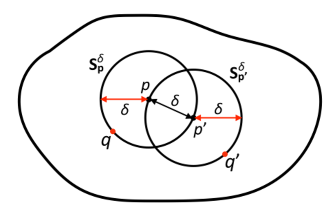
Figure 1: The quantum Ricci curvature $K(p,p^{\prime})$ is extracted from the computation of the average sphere distance (1) of two overlapping spheres $S_{p}^{\delta}$ and $S_{p^{\prime}}^{\delta}$ of radius $\delta$, whose centres $p$ and $p^{\prime}$ are a distance $\delta$ apart.

To extract $K(p,p^{\prime})$ one computes the average sphere distance $\bar{d}(S_{p}^{\delta},S_{p^{\prime}}^{\delta})$, which by definition is given by the normalized double-integral

$$\bar{d}(S_{p}^{\delta},S_{p^{\prime}}^{\delta}):=\frac{1}{\textit{vol}\,(S_{p}^{\delta})}\frac{1}{\textit{vol}\,(S_{p^{\prime}}^{\delta})}\int_{S_{p}^{\delta}}dq\;\sqrt{h}\int_{S_{p^{\prime}}^{\delta}}dq^{\prime}\;\sqrt{h^{\prime}}\ d_{g}(q,q^{\prime})$$ (1)

over all pairs of points $(q,q^{\prime})\in S_{p}^{\delta}\times S_{p^{\prime}}^{\delta}$, that is, by averaging the distance $d_{g}(q,q^{\prime})$ over the two circles, where $h$ and $h^{\prime}$ are the determinants of the induced metrics on $S_{p}^{\delta}$ and $S_{p^{\prime}}^{\delta}$, which are also used to compute the one-dimensional circle volumes $vol(S)$. From eq. (1), the quantum Ricci curvature $K(p,p^{\prime})$ associated with the point pair $(p,p^{\prime})$ is defined by

$$\bar{d}(S_{p}^{\delta},S_{p^{\prime}}^{\delta})/\delta=c\,(1-K(p,p^{\prime})),\;\;\;\;\;\;\;\;\delta=d_{g}(p,p^{\prime}),$$ (2)

where the prefactor $c$ is given by $c\!:=\!\lim_{\delta\rightarrow 0}\bar{d}/\delta$, and in general may depend on the point $p$. On smooth Riemannian manifolds and for small distances $\delta$, one can expand the quotient (2) into a power series in $\delta$, with $c$ a constant that only depends on the dimension. In two dimensions, one finds [12]

$$\bar{d}/\delta=1.5746+\delta^{2}\left(-0.1440\,\textit{Ric}(v,v)+{\cal O}(\delta)\right),$$ (3)

where $\mathit{Ric}(v,v)\!=\!R_{ij}v^{i}v^{j}$ is the usual Ricci curvature, evaluated on the unit vector $v$ at the point $p$ in the direction of $p^{\prime}$, and the numerical coefficients are rounded to the digits shown.

To obtain a global observable of the type discussed in Sec. 1, we integrate the average sphere distance (1) over all positions $p$ and $p^{\prime}$ of the two circle centres, while keeping their distance $\delta$ fixed. The spatial average over the average sphere distance at the scale $\delta$ is

$$\bar{d}_{\rm av}(\delta):=\frac{1}{Z_{\delta}}\int_{M}d^{2}x\sqrt{g}\int_{M}d^{2}x^{\prime}\sqrt{g}\;\,\bar{d}(S_{x}^{\delta},S_{x^{\prime}}^{\delta})\;\delta_{D}(d_{g}(x,x^{\prime}),\delta),$$ (4)

where $\delta_{D}$ denotes the Dirac delta function and the normalization factor $Z_{\delta}$ is given by

$$Z_{\delta}=\int_{M}d^{2}x\sqrt{g}\int_{M}d^{2}x^{\prime}\sqrt{g}\;\;\delta_{D}(d_{g}(x,x^{\prime}),\delta).$$ (5)

The integration in eq. (4) includes an averaging over directions, which means that it will allow us to extract an (averaged) quantum Ricci scalar $K_{\rm av}(\delta)$. The curvature profile is now given by the quotient

$$\bar{d}_{\rm av}(\delta)/\delta=:c_{\rm av}(1-K_{\rm av}(\delta)),$$ (6)

where the constant $c_{\rm av}$ is defined by $c_{\rm av}\!:=\!\lim_{\delta\rightarrow 0}\bar{d}_{\rm av}/\delta$. Note that for the special case where $M$ is the round two-sphere no spatial averaging is necessary to obtain the curvature profile [11], because in that case the average sphere distance (1) depends only on the distance $\delta$, and not on the locations of $p$ and $p^{\prime}$.

Although in the above discussion we have concentrated on the case of two dimensions, an analogous construction goes through in higher dimensions too. As emphasized in the introduction, the classical curvature profile (6) can be translated directly into a quantum observable, whose expectation value $\langle\bar{d}_{\rm av}(\delta)/\delta\rangle$ can be determined numerically in an approach like CDT quantum gravity. In such a lattice approach, all distances are given in dimensionless lattice units, which can be converted into dimensionful units invoking the lattice spacing $a$, an ultraviolet length cutoff that is taken to zero in any continuum limit. From the dimensionless curvature $K_{\rm av}(\delta)$ measured in the nonperturbative quantum theory one can extract a dimensionful, renormalized quantum Ricci scalar $K^{r}\!(\delta_{\rm ph})$, which depends on a physical coarse-graining or renormalization scale $\delta_{\rm ph}\!:=\!a\delta$, via

$$K_{\rm av}(\delta)=:\delta^{2}a^{2}K^{r}\!(\delta_{\rm ph})=(\delta_{\rm ph})^{2}K^{r}\!(\delta_{\rm ph}),$$ (7)

in the limit $a\rightarrow 0$. However, as discussed in the introductory section, in this work we will only be interested in the curvature profiles of certain classical spaces, where lengths and volumes vary continuously without any short-distance cutoff. As a preparation, we will in the next section examine the influence of a conical singularity on the average sphere distance (1) in two dimensions.

3 The influence of conical singularities

From the point of view of its intrinsic geometric properties, the surface of a regular tetrahedron is flat everywhere, apart from its corners, where curvature is concentrated in the manner of a delta function. The curvature that appears along its edges (with the exception of the four corners) in a standard embedding picture of the tetrahedron in Euclidean $\mathbb{R}^{3}$ is only extrinsic and not of interest in our present context. The same is true for the surfaces of other regular polyhedra. It implies that the intrinsic geometry of the neighbourhood of any of their corners is identical to that of a cone with a conical curvature singularity at its “tip”. To obtain the curvature profile of such a classical two-dimensional space, we must understand how the presence of one or more conical singularities affects the average sphere distance of a pair of circles on them.

Our quantitative assessment starts by examining the influence of a single conical singularity. Clearly, since the metric of a cone is flat everywhere except at the point where the singularity is located, if the pair $(S_{p}^{\delta},S_{p^{\prime}}^{\delta})$ of $\delta$-circles depicted in Fig. 1 is sufficiently far away from the singularity, the normalized average sphere distance is that of flat space, $\bar{d}(S_{p}^{\delta},S_{p^{\prime}}^{\delta})/\delta\!\approx\!1.5746$. On the other hand, if the conical singularity lies somewhere inside the double circle, one would expect it to have a nontrivial effect. However, somewhat contrary to naïve expectation, the curvature singularity has an influence on the average sphere distance even when it lies strictly outside the two circles, as long as it is sufficiently close to them. As we will show in more detail below, this is due to the presence of “geodesic shortcuts” associated with the conical singularity.

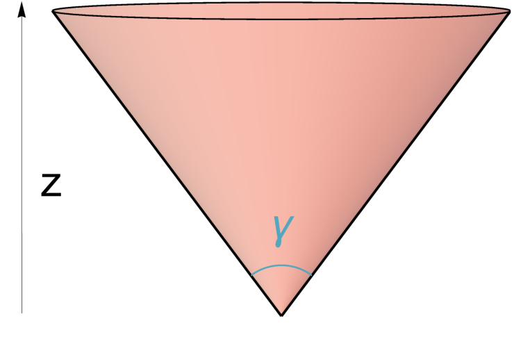
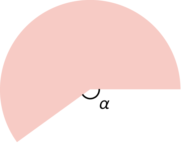
Figure 2: A geometry with a conical singularity can be represented as a cone in Euclidean space with apex angle $\gamma$ (left) or a flat plane with an angle $\alpha$ removed (right).

3.1 Geometry of the cone

One way of describing a cone with apex angle $\gamma$ is as the set of all points $(x,y,z)\in\mathbb{R}^{3}$ satisfying $z\!=\!\cot(\gamma/2)\sqrt{x^{2}+y^{2}}$, where $0\!<\!\gamma\!\leq\!\pi$ (Fig. 2, left). The apex or tip of the cone lies at the origin of the Cartesian coordinate system, and $\gamma$ is the angle formed in the plane $x\!=\!0$ by its intersection with the cone. A point on the cone can be labelled by its Euclidean distance $r$ to the origin and a rotation angle $\theta=\arctan y/x\in[0,2\pi]$. The induced metric on the cone in terms of these coordinates is given by

$$ds^{2}=dr^{2}+\sin^{2}(\tfrac{\gamma}{2})\,r^{2}\,d\theta^{2}.$$ (8)

An alternative description of the cone is obtained by cutting out an infinite wedge with angle $\alpha$ from the Euclidean plane $\mathbb{R}^{2}$ (Fig. 2, right) and identifying boundary points pairwise across the wedge. The result is a cone with a curvature singularity characterized by the deficit angle $\alpha$, which is a direct measure of Gaussian curvature. Since we are only interested in singularities with positive curvature, the relevant angle range is $0\!\leq\!\alpha\!<\!2\pi$. The relation with the apex angle $\gamma$ is $\alpha=2\pi(1-\sin(\gamma/2))$.

The useful feature of the “planar” representation of the cone in terms of a part of $\mathbb{R}^{2}$ is the fact that geodesics are simply given by straight lines. A knowledge of geodesics is needed to determine the geodesic distances between points. The only minor difficulty one has to take care of is to continue a geodesic correctly across the wedge if necessary. Placing the singularity at the origin of $\mathbb{R}^{2}$ and using standard spherical coordinates $(r,\varphi)$, the metric on the cone in this parametrization is

$$ds^{2}=dr^{2}+r^{2}d\varphi^{2},$$ (9)

where the range of the angle $\varphi$ is limited to $\varphi\in[0,2\pi-\alpha]$. Using the notation $r$ is justified, because the radial geodesic distance here is identical to the one we used for the cone embedded in $\mathbb{R}^{3}$. Comparing the two metrics (8) and (9), we see that they are simply related by a constant rescaling of the angles $\theta$ and $\varphi$, namely, $\varphi=\sin(\gamma/2)\theta$. The distance between two points $(r_{1},\varphi_{1})$ and $(r_{2},\varphi_{2})$ is simply their Euclidean distance

$$d\left((r_{1},\varphi_{1}),(r_{2},\varphi_{2})\right)=\sqrt{r_{1}^{2}+r_{2}^{2}-2r_{1}r_{2}\cos(\varphi_{2}-\varphi_{1})},$$ (10)

whenever the absolute angle difference $|\varphi_{2}-\varphi_{1}|$ does not exceed $\pi-\alpha/2$. If it does, the argument of the cosine should be substituted by the angle $2\pi-\alpha-|\varphi_{2}-\varphi_{1}|$. By rescaling the angles, we can immediately derive a distance function for points on the cone labelled by $r$ and $\theta$, namely,

$$d\left((r_{1},\theta_{1}),(r_{2},\theta_{2})\right)=\sqrt{r_{1}^{2}+r_{2}^{2}-2r_{1}r_{2}\cos(\sin(\tfrac{\gamma}{2})\Delta(\theta_{1},\theta_{2}))},$$ (11)

where

$$\Delta(\theta_{1},\theta_{2}):=\min(|\theta_{2}-\theta_{1}|,2\pi-|\theta_{2}-\theta_{1}|).$$ (12)

In what follows, we will work with the cone parametrization in terms of coordinates $(r,\theta)$, which is more convenient in the applications we will consider.

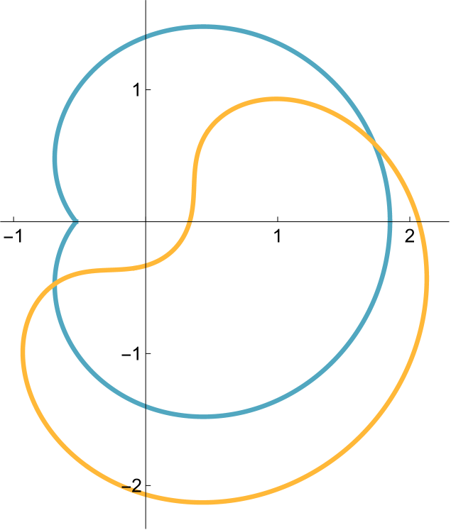
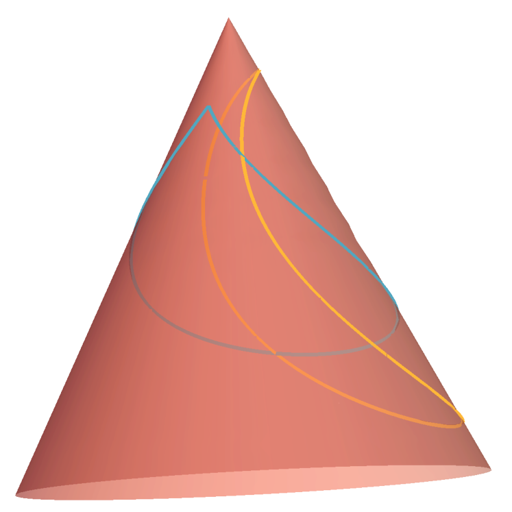
Figure 3: Two unit circles in the $(r,\theta)$-plane with a singularity at the origin (left), and on the cone embedded in $\mathbb{R}^{3}$ (right). The blue circle encloses the singularity and shows a discontinuous jump of its tangent vector at $\theta=\pi$.

3.2 Computing average sphere distances

To compute the average sphere distances (1) on the cone $M$, we must first parametrize geodesic circles on $M$, where the geodesic circle of radius $\delta$ centred at the point $p$ consists of all points $q$ at distance $\delta$ from $p$, $S_{p}^{\delta}=\{q\in M|\,d(p,q)\!=\!\delta\}$. Let us first discuss the parametrization of a geodesic circle which encloses the singularity at the origin. This case is slightly simpler, because the angle $\theta$ of $M$ can be used to label the points of $S_{p}^{\delta}$ uniquely. Using the rotational invariance of the set-up, we can without loss of generality choose the centre $p$ to have coordinates $p=(r_{1},\theta_{1}\!=\!0)$, where $r_{1}<\delta$. Labelling a point $q$ on the circle $S_{p}^{\delta}$ by $q=(r_{2},\theta_{2})$, it must by assumption satisfy $d(p,q)\!=\!\delta$, which is a quadratic equation for $r_{2}$. Because of relation (12), we should distinguish between the cases $0\leq\theta_{2}\leq\pi$ and $\pi\leq\theta_{2}\leq 2\pi$. The unique solutions $r_{2}(\theta_{2})$ are

$$r_{2}(\theta_{2})\!=\!\begin{cases}r_{1}\cos\!\left(\theta_{2}\sin(\frac{\gamma}{2})\right)\!+\!\sqrt{\delta^{2}\!-\!r_{1}^{2}\sin^{2}\!\left(\theta_{2}\sin(\frac{\gamma}{2})\right)},\;\;\;&0\leq\theta_{2}\leq\pi,\\ r_{1}\cos\!\left((2\pi\!-\!\theta_{2})\sin(\frac{\gamma}{2})\right)\!+\!\sqrt{\delta^{2}\!-\!r_{1}^{2}\sin^{2}\!\left((2\pi\!-\!\theta_{2})\sin(\frac{\gamma}{2})\right)},&\pi\leq\theta_{2}\leq 2\pi.\end{cases}$$ (13)

They can be used to uniquely parametrize the points along $S_{p}^{\delta}$ by the curve

$$c^{\mu}(\theta)=(r_{2}(\theta),\theta),\;\;\;\;\;0\leq\theta\leq 2\pi,$$ (14)

with curve parameter $\theta$, and where for ease of notation we have suppressed the dependence of the curve on $p$ and $\delta$. Note that this curve is smooth everywhere apart from the point $\theta\!=\!\pi$, where its tangent vector $dc^{\mu}/d\theta$ jumps in a discontinuous way, resulting in a kink in the curve $c(\theta)$ (Fig. 3). If the centre $p$ has coordinates $(r_{1},\theta_{1})$, for some nonvanishing angle $\theta_{1}$, the angle $\theta_{2}$ on the right-hand sides of the relations (13) should be substituted by $|\theta_{2}-\theta_{1}|$.

The parametrization of a geodesic circle which does not enclose the curvature singularity can also be parametrized by a $\theta$-angle, but not uniquely. As we will see below, a convenient choice in any integration along $S_{p}^{\delta}$ is to parametrize the circle along two separate segments and then add their contributions. Again we choose the point $p=(r_{1},0)$ as the centre of the circle, whose radial coordinate now satisfies $r_{1}\geq\delta$. When solving the equation $d(p,q)\!=\!\delta$ for $r_{2}$ as before, there are two differences. First, the angle $\theta_{2}$ can only vary in the interval $[-\theta_{\rm m},\theta_{\rm m}]$, where the maximal angle $\theta_{m}$ is defined by $\sin(\sin{(\gamma/2)}\,\theta_{\rm m})\!=\!\delta/r_{1}$. This is easy to see by examining the geometry of the situation in the flat-space coordinates $(r,\varphi)$. Second, there are two solutions $r_{2}(\theta_{2})$ for every value $\theta_{2}$ in the interior of this interval, namely,

$$r^{\pm}_{2}(\theta_{2})=r_{1}\cos\!\left(\theta_{2}\sin(\tfrac{\gamma}{2})\right)\!\pm\!\sqrt{\delta^{2}\!-\!r_{1}^{2}\sin^{2}\!\left(\theta_{2}\sin(\tfrac{\gamma}{2})\right)},\;\;-\theta_{\rm m}\leq\theta_{2}\leq\theta_{\rm m}.$$ (15)

One easily verifies that the argument of the square root cannot become negative in the angle range considered. A straightforward way to parametrize the points $q$ along the circle is by splitting the circle into two segments $c_{+}(\theta)$ and $c_{-}(\theta)$, corresponding to the two solutions (15), namely,

$$c_{+}^{\mu}(\theta)=\left(r_{2}^{+}(\theta),\theta\right),\;\; -\theta_{\rm m}\leq\theta\leq\theta_{\rm m},$$ (16)

$$c_{-}^{\mu}(\theta)=\left(r_{2}^{-}(\theta),\theta\right),\;\; -\theta_{\rm m}\leq\theta\leq\theta_{\rm m}.$$ (17)

If the angle $\theta_{1}$ of the point $p\!=\!(r_{1},\theta_{1})$ is nonvanishing, the angles $\theta_{2}$ in the above expressions should again be substituted appropriately. As a cross check of the circle parametrizations, one can use them to compute the lengths (one-dimensional volumes) of the circles, which at any rate are needed in the computation of the average sphere distances (1). For the case that the circle encloses the singularity, one finds

$$vol(S^{\delta}_{p}) =\int_{0}^{2\pi}\!\!\!d\theta\,\sqrt{g_{\mu\nu}\tfrac{dc^{\mu}}{d\theta}\tfrac{dc^{\nu}}{d\theta}}$$

$$=\int_{0}^{\pi}\!d\theta\,\delta\sin(\tfrac{\gamma}{2})(1\!+\!{\cal R}(\theta))+\!\int_{\pi}^{2\pi}\!\!\!d\theta\,\delta\sin(\tfrac{\gamma}{2})(1\!+\!{\cal R}(2\pi-\theta))$$ (18)

$$=2\pi\delta\sin(\tfrac{\gamma}{2})+2\delta\arcsin\left(\tfrac{r_{1}}{\delta}\sin\left(\pi\sin(\tfrac{\gamma}{2})\right)\right),\hskip 71.13188pt[r_{1}<\delta]$$

where $g_{\mu\nu}$ refers to the metric (8) and we have introduced the shorthand notation

$${\cal R}(\theta)=\frac{r_{1}\cos\left(\theta\sin(\tfrac{\gamma}{2})\right)}{\sqrt{\delta^{2}-r_{1}^{2}\sin^{2}\left(\theta\sin(\tfrac{\gamma}{2})\right)}}.$$ (19)

For the case that the circle does not enclose the singularity, the corresponding computation yields

$$vol(S^{\delta}_{p}) =\int_{-\theta_{\rm m}}^{\theta_{\rm m}}\!\!\!d\theta\,\sqrt{g_{\mu\nu}\tfrac{dc^{\mu}_{+}}{d\theta}\tfrac{dc^{\nu}_{+}}{d\theta}}+\int_{-\theta_{\rm m}}^{\theta_{\rm m}}\!\!\!d\theta\,\sqrt{g_{\mu\nu}\tfrac{dc^{\mu}_{-}}{d\theta}\tfrac{dc^{\nu}_{-}}{d\theta}}$$

$$=\int_{-\theta_{\rm m}}^{\theta_{\rm m}}\!d\theta\,\delta\sin(\tfrac{\gamma}{2})(1\!+\!{\cal R}(\theta))+\!\int_{-\theta_{\rm m}}^{\theta_{\rm m}}\!\!\!d\theta\,\delta\sin(\tfrac{\gamma}{2})(-1\!+\!{\cal R}(\theta))$$ (20)

$$=2\pi\delta,\hskip 256.0748pt[r_{1}\geq\delta]$$

which is the expected flat-space result.

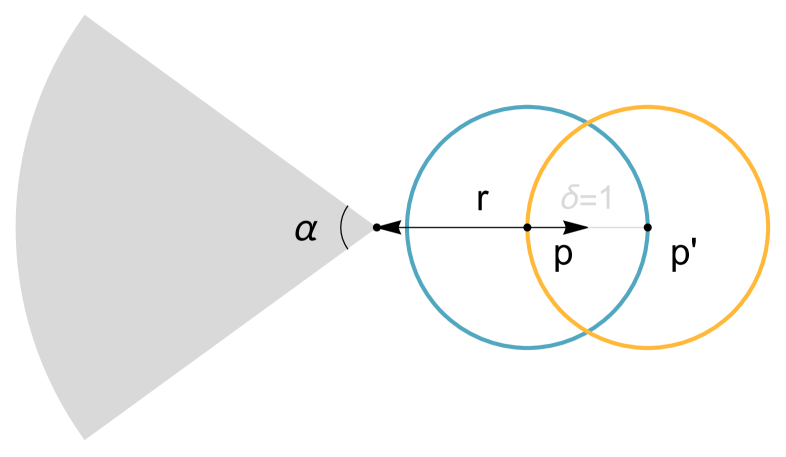
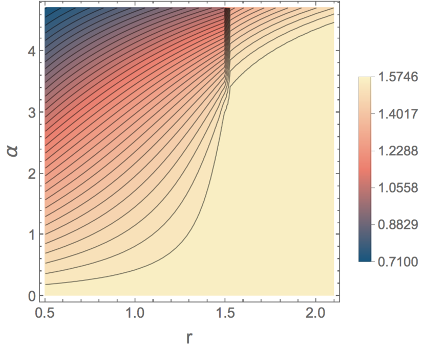
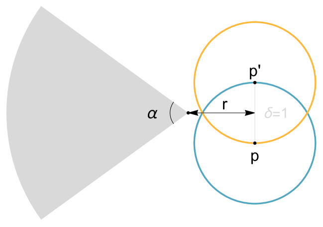
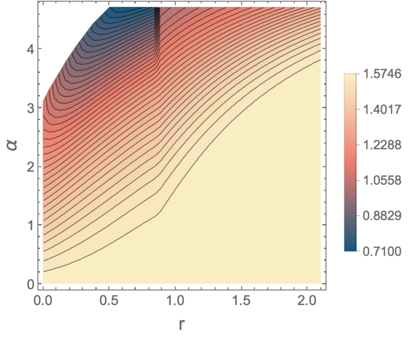
Figure 4: Contour plots of the average sphere distance $\bar{d}(S_{p}^{\delta},S_{p^{\prime}}^{\delta})$ as a function of $\alpha$ and $r$, for two particular circle arrangements, as described in the text. The distance $r$ is given in units of $\delta$ and the deficit angle $\alpha$ in radians.

We now have all ingredients in hand to explicitly compute the average sphere distance (1) for pairs $(p,p^{\prime})$ of points at distance $\delta$. We perform the double-integral numerically in Mathematica, where the intermediate accuracy is kept at 8 significant digits. Apart from the strength of the singularity (captured by the deficit angle $\alpha$) and the linear distance $\delta$, $\bar{d}(S_{p}^{\delta},S_{p^{\prime}}^{\delta})$ depends on the distance of $p$ from the singularity and on the orientation of the second circle relative to the first.

To illustrate the behaviour of $\bar{d}$, Fig. 4 shows contour plots for two particular orientations of the double circle relative to the singularity, where the average sphere distance is given as a function of the deficit angle $\alpha$ and the distance $r$ of the midpoint between $p$ and $p^{\prime}$ to the singularity. To fix the overall scale, we have set $\delta\!=\!1$. Recall that for $\alpha\!=\!0$, there is no singularity, and that in flat space $\bar{d}\!\approx\!1.5746$. As indicated by the darker shades in Fig. 4, the value of $\bar{d}$ decreases with increasing $\alpha$ and decreasing distance to the singularity, characteristic of a positive and growing quantum Ricci curvature. The illustrations of the circle positions use the planar representation of the cone with a wedge removed. In Fig. 4, left, the circle centres are chosen collinear with the singularity. For $r\!\geq\!1.5$, neither of the circles encloses the singularity and there is no or little deviation from the flat-space behaviour, unless $\alpha$ increases beyond $\pi$. In this case the wedge will “cut into” the first circle, giving rise to a nontrivial effect. The region $r\!<\!0.5$ is not well defined, since it would imply that $p$ lies inside the wedge. In Fig. 4, right, the two circles are arranged symmetrically with respect to the singularity. What is noteworthy here is the fact that even when the singularity lies outside the circle configuration, i.e. $r\!>\!\sqrt{3}/2\approx 0.866$, and the size of the deficit angle is only moderate, there is a nontrivial effect on $\bar{d}$. We will look closer at this phenomenon in the next subsection. The top left-hand corner of the contour plot is not defined, since both $p$ and $p^{\prime}$ would lie inside the wedge.

3.3 Domain of influence

So far, the developments of this section have been concerned with the geometry in the vicinity of an isolated curvature singularity on an infinitely extended cone. However, we are interested in determining the curvature profiles of compact, flat spaces with several such singularities, more precisely, the regular polyhedral surfaces of the so-called Platonic solids: the tetrahedron, octahedron, cube, dodecahedron and icosahedron. The method developed for computing average sphere distances on a cone can be used on these polyhedra too, but only if the double circles are sufficiently small to not be influenced by more than one of the conical singularities at the corners of these polyhedra. For a surface with a given area, determined by the length of an edge, this imposes an upper bound on the size $\delta$ of the circles. Since we need to average over all double circles of size $\delta$ to obtain the curvature profile, we must determine the size $\delta_{\rm max}$ below which the computation of $\bar{d}(S_{p}^{\delta},S_{p^{\prime}}^{\delta})$ will never be influenced by more than one of the corner points.

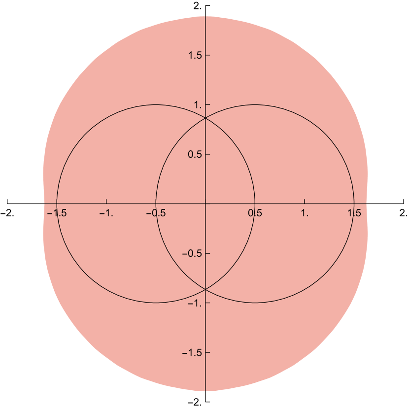
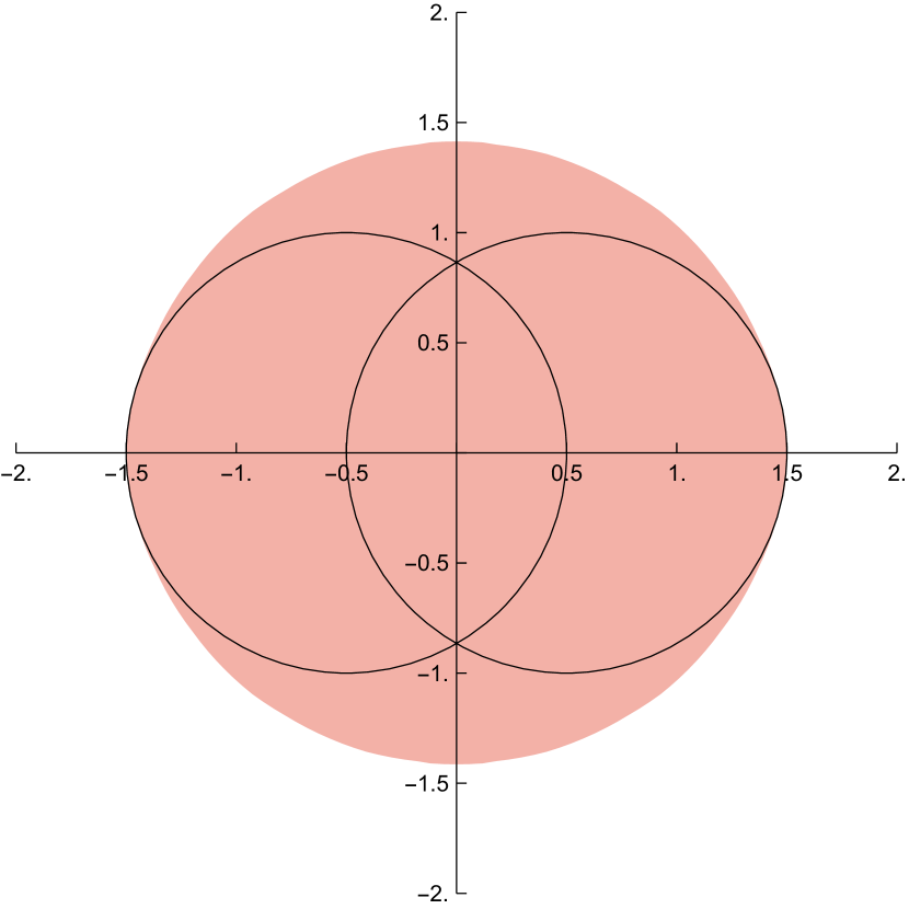
Figure 5: The domains of influence of a curvature singularity on the tetrahedron (left) and the octahedron (right).

This leads to the notion of the domain of influence of a curvature singularity with angle $\alpha$, defined as the open two-dimensional region, including and surrounding a circle pair $(S_{p}^{\delta},S_{p^{\prime}}^{\delta})$, which consists of all points where a singularity of strength $\alpha$ would cause $\bar{d}/\delta$ to deviate from its flat-space value. Fig. 5 illustrates the situation for $\alpha\!=\!\pi$ and $\alpha\!=\!2\pi/3$, associated with the deficit angles on the tetrahedral and octahedral surfaces respectively. The reason why a curvature singularity can influence the average sphere distance, even when it lies outside either of the circles, is twofold. Firstly, a geodesic between a pair $(q,q^{\prime})$ of points from the two circles can of course pass through a region that lies outside the circles and be influenced by a singularity located there. Secondly, because of the presence of the singularity, geodesics between points will not always be unique, but can occur in pairs that pass on either side of the singularity. This can lead to a geodesic shortcut between given points $q$ and $q^{\prime}$, compared with the situation in flat space.

The relevant quantity we need to determine for our purposes is the maximal diameter of the domain of influence for a given angle $\alpha$. When measuring the curvature profile with the method described above, we must make sure that this diameter does not exceed the edge length $L$ of the given polyhedron, which is the same as the distance between neighbouring singularities. If we call ${\cal D}(\alpha)$ the maximal diameter in units of $\delta$, it follows that the largest allowed circle size is $\delta_{\rm max}\!=\!L/{\cal D}(\alpha)$. The maximal diameter for the tetrahedral surface can be determined from geometric considerations and is given by ${\cal D}(\pi)\!=\!\sqrt{9+4\sqrt{2}}\!\approx\!3.828$, corresponding to the vertical axis in the left diagram of Fig. 5. As the deficit angle $\alpha$ decreases towards $2\pi/3$, the domain of influence shrinks along both axes until it reaches the left- and rightmost points of the double circle. The domain keeps shrinking along the vertical axis to a value below 3 (Fig. 5, right). It cannot shrink further along the horizontal direction since a singularity inside one (or both) of the circles always leads to a nonflat result for $\bar{d}/\delta$. We conclude that for the octahedron and the remaining platonic solids with $\alpha\!=\!\pi/2$, $\pi/3$ and $\pi/5$, we have ${\cal D}(\alpha)\!=\!3$.

4 Measuring curvature profiles

The insights gained above will now be applied to evaluate curvature profiles for the surfaces of the five convex regular polyhedra depicted in Table 1. Each surface consists of identical polygons, whose edges have all the same length. Its Gaussian curvature is distributed equally over all vertices, which implies that each deficit angle has size $\alpha\!=\!4\pi/\#$vertices. Since we are interested in the effectsof how the same amount of curvature is distributed over a given spatial volume, we compare the results for surfaces of the same area, which we take to be $4\pi$, the area of a two-sphere of unit radius. The resulting values for the edge lengths $L$ and the associated maximal circle radii $\delta_{\rm max}$ can be found in Table 1.

Platonic solid	surface	elementary region	$\#$ vertices	$\#$ edges	$\#$ faces	$L$	$\delta_{\rm max}$
tetrahedron			4	6	4	2.694	0.7036
octahedron			6	12	8	1.905	0.6349
cube			8	12	6	1.447	0.4824
icosahedron			12	30	20	1.205	0.4015
dodecahedron			20	30	12	0.780	0.2601

Table 1: Polyhedral surfaces of the Platonic solids, with some of their properties.

From the limits on $\delta$ it is clear that we will only obtain partial curvature profiles. It is not straightforward to extend the present method to include a second conical singularity, and we have not attempted to do so. However, it turns out that for the special case of the tetrahedral surface there is an alternative way to extend the $\delta$-range significantly, as will be discussed in Sec. 5 below. The reason is that one can attain a good and computationally explicit control over its geodesics.

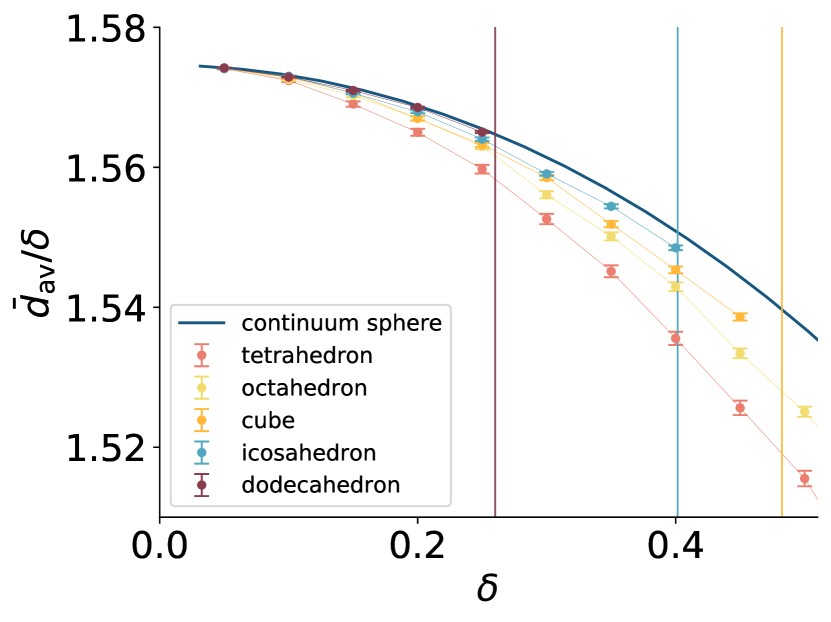
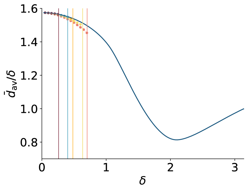
Figure 6: Measurements of the curvature profiles $\bar{d}_{\rm av}(\delta)/\delta$ of the surfaces of the five Platonic solids, compared to that of the continuum sphere of the same area (top curve), plotted in the $\delta$-ranges $[0,0.5]$ (left) and $[0,\pi]$ (right). (Line segments connecting data points are merely to guide the eye.)

To compute the spatial average of the average sphere distance on a given polyhedral surface, we use a uniform sampling with respect to the flat metric (disregarding the singular points), somewhat similar to what has been done in a quantum context [12, 13]. Because of the discrete symmetries of the polyhedra, it suffices to pick the first circle centre $p$ of a double-circle configuration from what we will call an elementary region. This is a triangular subregion of a face, whose corners are given by the midpoint of an edge, one of the endpoints of the same edge (a singular vertex) and the midpoint of the face, as indicated in Table 1. The data for a given value of $\delta\in\,]0,\delta_{\rm max}]$ are collected as follows:

1. Sprinkle $n$ points $p_{i}$, $i\!=\!1,\dots,n$, randomly and uniformly into an elementary region.

2. Construct geodesic circles $S^{\delta}_{p_{i}}$, using the parametrizations found in Sec. 3.2.

3. For every $p_{i}$, pick a point $p^{\prime}_{i}$ on $S^{\delta}_{p_{i}}$ uniformly at random, and construct the geodesic circle $S^{\delta}_{p^{\prime}_{i}}$ around it.

4. Compute $\bar{d}(S_{p_{i}}^{\delta},S_{p^{\prime}_{i}}^{\delta})$ for all pairs $(p_{i},p^{\prime}_{i})$.

5. Average over the results to obtain $\bar{d}_{\rm av}(\delta)$.

We have collected 10.000 measurements for each data point, with a step size of $\delta\!=\!0.05$. The results for the curvature profiles $\bar{d}_{\rm av}/\delta$ for the five regular polyhedra are shown in Fig. 6, together with the curvature profile of the continuum two-sphere for comparison. On the left, we show the behaviour at small distances $\delta\!\lesssim\!0.5$. It is clearly distinct for the five spaces, but qualitatively similar. (The vertical lines indicate the cutoff values $\delta_{\rm max}$ for the various cases.) The data for the dodecahedron resemble those of the continuum sphere most closely, at least within the limited $\delta$-range considered. Generally speaking, the larger the number of vertices over which the deficit angles are distributed, the closer is the match with the sphere curve. Note also that all curves seem to converge to the flat-space value as $\delta\rightarrow 0$, as one would expect.

In Fig. 6, right, we have zoomed out for a more global comparison with the curvature profile of the sphere in the range $\delta\in[0,\pi]$. As mentioned above, we will in the following section introduce a different method to determine geodesic circles on the tetrahedron, which will allow us extend its curvature profile over most of the range depicted here. Based on the limited data presented here, we conclude that the averaged quantum Ricci curvature of all the investigated spaces is positive, which is not surprising. It is largest for the tetrahedron, for which the decrease of the curve for $\bar{d}_{\rm av}(\delta)/\delta$ is steepest.

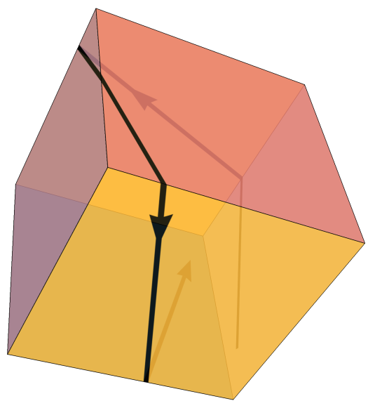
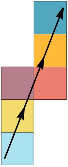
Figure 7: Geodesic on a cube (left) and its corresponding development in the plane (right).

5 Unfolding the tetrahedron

The study of geodesics on regular convex polyhedra, and the classification of closed geodesics in particular, is an active area of mathematical research (for example, see [19, 20]). Our primary interest are shortest geodesics between arbitrary pairs of points, a problem that is most straightforwardly tackled for the tetrahedron. This is fortunate, since the tetrahedron is the most interesting case from our point of view. Of all the Platonic solids, its curvature is distributed least homogeneously, while the results on the curvature profiles of the previous section suggest that all other cases lie in between those of the tetrahedron and the smooth sphere.

A general technique one can use to study geodesics on regular polyhedra is by “rolling” or “unfolding” the polyhedron onto the flat two-dimensional plane along a given geodesic. The so-called development of a polyhedron along a geodesic proceeds as follows [19]: starting from an arbitrary point $p$ contained in some face $F_{0}$ of the polyhedral surface and an initial direction, one follows the corresponding geodesic (straight line) in $F_{0}$ until it hits an edge to a neighbouring face $F_{1}$. Since all faces are flat, the adjacent pair of $F_{0}$ and $F_{1}$ can in an isometric way be put down in the plane. Following the geodesic as it passes through $F_{1}$, it will meet another edge to some neighbouring face $F_{2}$, which likewise can be folded out into the plane, and so forth. The result of this development is a contiguous chain of faces in the plane, which is traversed by the geodesic, taking the form of a straight line. Fig. 7 illustrates the procedure for a geodesic running along the surface of a cube. The six sides of the cube have a different colour coding and will in general appear repeatedly along a given geodesic.

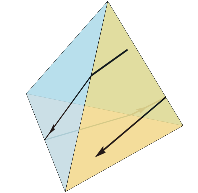
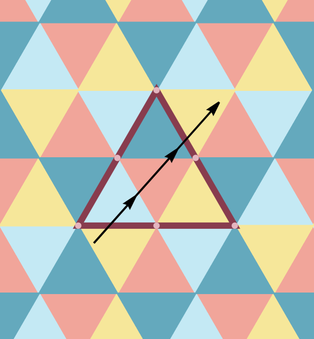
Figure 8: Geodesic on a tetrahedron (left) and its development in the plane, which forms part of a regular tiling in terms of the four faces of the tetrahedron (right). The thick line encloses a fundamental domain $\cal F$.

The tetrahedron is special among the regular polyhedra in the sense that it has an everywhere consistent development, which is independent of the geodesic chosen. The full development in all directions constitutes a regular tessellation of the flat plane by equilateral triangles, which come in four types or colours, corresponding to the four faces of the tetrahedron. Fig. 8 shows an example of a geodesic on the tetrahedron and the corresponding straight line in the regular tiling. We have also indicated a triangle-shaped fundamental domain $\cal F$, consisting of four triangles that make up a single copy of the tetrahedron. The plane can also be thought of as a tessellation by copies of $\cal F$ with alternating orientation, either with the orientation shown in the figure or an upside-down version rotated by 180 degrees. This planar set-up will allow us to construct geodesic circles and compute average sphere distances for radii $\delta$ of up to one tetrahedral edge length, which is almost four times the range we could cover with the previous method.

5.1 Geodesic circles on the tetrahedron

The new representation in terms of unfolded tetrahedra allows us relatively easily to determine geodesic circles that enclose more than one singularity. A more elementary step we need to understand first is how to determine the distance between two arbitrary points $p$ and $q$ on the surface of the tetrahedron, which is given by the length of the shortest geodesic between them. Let us represent the surface by the fundamental domain $\cal F$ of Fig. 8. Because of the symmetries of the tetrahedron, we can without loss of generality choose the point $p$ to lie in (or on the boundary of) the elementary triangular region in the central triangle of $\cal F$. The second point $q$ can be located anywhere in $\cal F$ (Fig. 9, left). The key observation now is that the unique straight line one can draw from $p$ to $q$ in $\cal F$ clearly corresponds to a geodesic on the tetrahedron, but not necessarily the shortest one. This can happen because the tetrahedral surface is obtained by appropriate pairwise identifications of the six boundary edges of the domain $\cal F$, and the shortest geodesic to $q$ may cross one or more of these boundaries. One

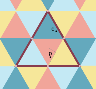
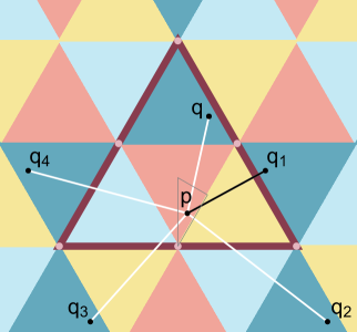
Figure 9: Fundamental domain $\cal F$ with a point $p$ in the elementary region of the centre triangle of $\cal F$, and a second point $q$ (left). To determine the distance between $p$ and $q$, we must consider copies $q_{i}$ of the point $q$ in neighbouring copies of $\cal F$ (right). The shortest line is drawn in black.

can easily find this geodesic by going back to the tessellation of the plane and considering a sufficiently large neighbourhood of the fundamental domain $\cal F$, consisting of $\cal F$ itself and neighbouring copies ${\cal F}_{i}$, $i\!=\!1,2,\dots$, of $\cal F$. On each of these copies, we mark the unique copy $q_{i}$ of the point $q$ (Fig. 9, right). The length of the shortest straight line between $p$ and either $q$ or any of the $q_{i}$ is the searched-for geodesic distance between $p$ and $q$.

This way of representing the tetrahedron and its geodesics is not unlike our previous representation of the geometry of an isolated conical singularity in terms of a plane with a wedge removed: the nature of the geodesics is maximally simple (straight lines), but one pays a price in the form of nontrivial identifications.

Building on the above insight on how geodesic distances are determined, we next discuss the nature of geodesic circles of radius $\delta$ based at a point $p$. It is best illustrated by referring to the convex set ${\cal C}_{p}$ of all points $q$ in the tessellated plane, for given $p$ in the elementary region, which are closer to $p$ than any of their copies (in $\cal F$ or any of the ${\cal F}_{i}$). To construct ${\cal C}_{p}$, one needs to recall the status of vertices in the tessellated plane. On the original tetrahedron, they corresponded to singularities with a deficit angle $\alpha\!=\!\pi$. Cutting open the tetrahedron along three of its edges and putting it in the plane results in a copy of the fundamental domain $\cal F$, which can be thought of as a region in the plane with three such wedges removed. Since all wedges have an angle $\pi$, one fundamental domain can be glued into another’s “missing wedge”. Repeating this gluing throughout the plane leads to a tiling of the plane which preserves all neighbourhood relations between pairs of tetrahedral faces sharing a common edge. What is not preserved is the number of faces meeting at a given vertex, which is three on the original tetrahedron and six in the plane.

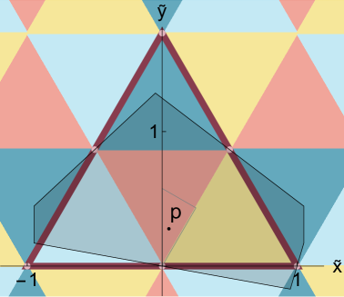
Figure 10: The convex polygon ${\cal C}_{p}$ superimposed on the tessellated plane. The axes show the orthonormal coordinate system $(\tilde{x},\tilde{y})$ used to construct the region.

The region ${\cal C}_{p}$ in the tessellated plane can be constructed from symmetry considerations. For a general point $p$ inside the elementary region, its boundary is a convex polygon with six corner points $S_{i}$, $i\!=\!1,\dots,6$. Its sides are formed by four straight line segments through the four vertices closest to $p$, where each line segment is perpendicular to the line from $p$ to the vertex in question. In addition, there are two parallel lines (vertical lines in Fig. 10) equidistant from $p$, which get mapped onto each other by one of the translation symmetries of the tessellated plane. Note that by construction the area of ${\cal C}_{p}$ is the same as the surface area of the tetrahedron.

To arrive at a quantitative description, we introduce an orthonormal coordinate system $(\tilde{x},\tilde{y})$ in the plane, whose origin $(0,0)$ is the midpoint between the two bottom edges of the fundamental domain $\cal F$ (Fig. 10). For definiteness, let us assume that all edges have unit length, $L\!=\!1$. Note that the elementary triangular region, which by assumption contains the point $p\!=\!(x,y)$, is spanned by the three corner points $(0,0)$, $(0,1/\sqrt{3})$ and $(1/4,\sqrt{3}/4)$, which means that the ranges of $x$ and $y$ are limited to $x\!\in\![0,1/4]$ and $y\!\in\![0,1/\sqrt{3}]$. In this coordinate system, the coordinates of the corner points of the region ${\cal C}_{p}$ are given by

$$S_{1}\!=\!\Big{(}x-1,\frac{x(1\!-\!x)}{y}\Big{)},\;S_{2}\!=\!\Big{(}x-1,\tfrac{1}{2}\big{(}\sqrt{3}-\frac{1-4x^{2}}{\sqrt{3}\!-\!2y}\big{)}\!\Big{)},\;S_{3}\!=\!\Big{(}-x,\tfrac{1}{2}\big{(}\sqrt{3}+\frac{1-4x^{2}}{\sqrt{3}\!-\!2y}\big{)}\!\Big{)},$$

$$S_{4}\!=\!\Big{(}x+1,\tfrac{1}{2}\big{(}\sqrt{3}-\frac{1-4x^{2}}{\sqrt{3}\!-\!2y}\big{)}\!\Big{)},\;S_{5}\!=\!\Big{(}x+1,\frac{x(1\!-\!x)}{y}\Big{)},\;S_{6}\!=\!\Big{(}1-x,-\frac{x(1\!-\!x)}{y}\Big{)},\;$$ (21)

for $y\not=0$, and by

$$S_{1}\!=\!(-1,0),\;S_{2}\!=\!\Big{(}\!-1,\frac{1}{\sqrt{3}}\Big{)},\;S_{3}\!=\!\Big{(}0,\frac{2}{\sqrt{3}}\Big{)},\;S_{4}\!=\!\Big{(}1,\frac{1}{\sqrt{3}}\Big{)},\;S_{5}\!=\!S_{6}\!=\!(1,0),$$ (22)

for $y\!=\!0$. In the latter case, corresponding to $p\!=\!(0,0)$, ${\cal C}_{p}$ becomes a five-cornered polygon that is equal to one half of a regular hexagon.

We have now set the stage for analyzing geodesic circles $S_{p}^{\delta}$ centred at $p$. In what follows, we will exclude the case $p\!=\!(0,0)$, where the circle centre would coincide with a singularity of the tetrahedron. For added simplicity, we will also assume that $p$ lies in the interior of the elementary region, which is the generic case. An analogous treatment of points along the boundary is completely straightforward.

Since in an open neighbourhood of $p$ space is flat and Euclidean, for sufficiently small $\delta$ the set of points $S_{p}^{\delta}$ is an ordinary circle of radius $\delta$ and circumference $2\pi\delta$. As we increase $\delta$ continuously, this continues to be the case until the circle reaches the singularity closest to $p$, located at $(\tilde{x},\tilde{y})\!=\!(0,0)$, where it also meets the line segment that forms part of the boundary of ${\cal C}_{p}$. The corresponding circle radius is $\delta\!=\!\sqrt{x^{2}+y^{2}}$. As we increase $\delta$ further, we need to take into account the nontrivial deficit angle associated with the point $(0,0)$. It implies that the piece of line segment to one side of the vertex $(0,0)$ should be identified with the piece to the other side. For the circle of radius $\delta$ we draw in the tessellated plane, it means that the circle segment beyond this line segment is not part of $S_{p}^{\delta}$. The “circle” $S_{p}^{\delta}$ with radius $\delta\!>\!\sqrt{x^{2}+y^{2}}$ therefore has a length that is shorter than $2\pi\delta$. The story repeats itself when we increase $\delta$ further and $S_{p}^{\delta}$ meets the singularity at $(\tilde{x},\tilde{y})\!=\!(1/2,\sqrt{3}/2)$, which is second-closest to $p$. From this radius onwards, a second circle segment will be removed from the “naïve” circle we can draw around $p$ in the plane. The same happens when $S_{p}^{\delta}$ reaches and passes the remaining two singularities, at $(-1/2,\sqrt{3}/2)$ and $(-1,0)$ respectively.

Since the tetrahedron has a finite diameter, the size of $S_{p}^{\delta}$ must be zero above some maximal value of $\delta$, given by the distance of the point(s) furthest away from the given point $p$, the antipode(s) of $p$. In this context, it should be noted that the three points $S_{1}$, $S_{5}$ and $S_{6}$ of eq. (21) are equidistant to $p$, with distance $d_{1}$, as are the three points $S_{2}$, $S_{3}$ and $S_{4}$, with distance $d_{2}$. Which of the two distances is larger and therefore sets the upper limit for the radius $\delta$ depends on the location of $p$ in the elementary region. It turns out that the extremal cases of the closest and the furthest antipodes are associated with points $p$ on the boundary of the elementary region. The antipode is closest when $p$ lies in the middle of an edge, $p\!=\!(1/4,\sqrt{3}/4)$, in which case the antipode has distance $d_{1}\!=\!d_{2}\!=\!1$ and also lies in the middle of an edge. By contrast, the point $p$ with the most distant antipode, with $d_{1}\!=\!d_{2}\!=\!2/\sqrt{3}\approx\!1.155$, lies at the centre of a face, with $p\!=\!(0,1/\sqrt{3})$.

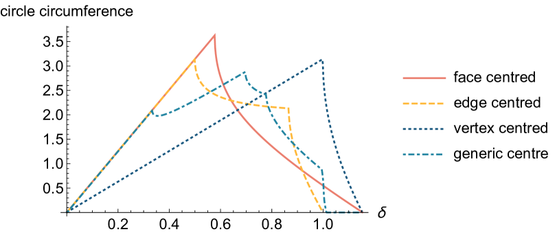
Figure 11: The circumference of geodesic circles $S_{p}^{\delta}$ on the tetrahedron as a function of the radius $\delta$, both in units of edge length, for various locations of the centre $p$.

These results are illustrated in Fig. 11, which shows the circumference of $S_{p}^{\delta}$ as a function of the geodesic radius $\delta$ for various choices of $p$. The computation is done by identifying which arcs of the “naïve” circle at radius $\delta$, parametrized by an ordinary rotation angle $\theta$, contribute to $S_{p}^{\delta}$ and by adding up the arc lengths. For all curves, we see an initial linear rise, characteristic of a circle in the flat plane, with the exception of $p$ at a vertex, for which the linear slope is flatter, corresponding to that of a cone with deficit angle $\pi$. For a generic location of the centre $p$, there subsequently are four cusps, corresponding to the radii where the circle $S_{p}^{\delta}$ meets one of the singularities, as discussed above. For non-generic $p$ some of the cusps can merge. When $p$ lies at the centre of an edge, it is clear that the two closest singularities are reached simultaneously at $\delta\!=\!0.5$, and the two remaining ones at $\delta\!=\!\sqrt{3}/2\!\approx\!0.866$. In this case, the antipode has the minimal distance 1 from $p$, which is why the curve in Fig. 11 stops at $\delta\!=\!1$. When $p$ lies at the centre of a face, the three closest singularities are reached simultaneously at $\delta\!=\!1/\sqrt{3}\!\approx\!0.577$, giving rise to a single cusp. The antipode, which in this case is maximally far away from $p$, coincides with the remaining vertex, and the corresponding curve ends at $\delta\!\approx\!1.155$. The same is true for the dual case, where the construction starts at a vertex. For comparison, the analogous curve for a smooth two-sphere of the same area as the tetrahedron would end at $\delta\!\approx\!1.166$.

The above analysis and Fig. 11 underline the strong inhomogeneity and anisotropy of the tetrahedral surface and at the same time fix an upper bound, $\delta\!=\!1$, up to which the notion of a geodesic circle $S_{p}^{\delta}$ is meaningful for arbitrary locations of $p$. This is relevant when we start taking spatial averages of average distances between circles of radius $\delta$ in order to obtain the curvature profile of the tetrahedron, which is the subject of the next section.

5.2 Computing the curvature profile

Putting together the construction of geodesic circles $S_{p}^{\delta}$ and our earlier observation about the need to choose the shortest geodesic between two points, we can now embark on computing average sphere distances for $\delta\!\in\![0,1]$ in units of edge length. To obtain a pair of overlapping circles $S_{p}^{\delta}$, $S_{p^{\prime}}^{\delta}$ for a given value of $\delta$, we start by picking a point $p$ randomly from the elementary region and constructing $S_{p}^{\delta}$, following the prescription of Sec. 5.1. In general, this will be given by a set of arcs in ${\cal C}_{p}$, parametrized by corresponding angle intervals in terms of the rotation angle $\theta$. To simplify subsequent computations, we map all arc sections that happen to lie in a neighbouring domain ${\cal F}_{i}$ back to the fundamental domain $\cal F$ by appropriate reflections and translations, which are symmetries of the tessellated plane (Fig. 12).

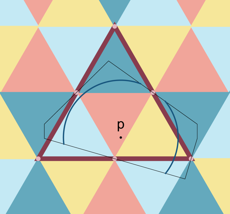
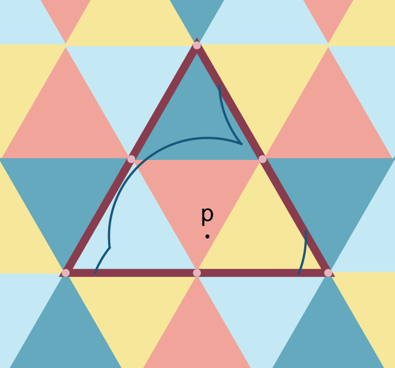
Figure 12: Constructing a geodesic circle on the tetrahedron (left) and mapping it inside the fundamental domain (right).

Next, we randomly pick a point $p^{\prime}$ on $S_{p}^{\delta}$, which will serve as the centre of the second circle $S_{p^{\prime}}^{\delta}$. We then again construct the arcs forming $S_{p^{\prime}}^{\delta}$ using a region similar to ${\cal C}_{p}$, where the center point $p^{\prime}$ is now generically not in the triangular elementary region. The analogous region ${\cal C}_{p^{\prime}}$ can be found by an appropriate symmetry transformation. In principle it would be possible to then map all arc sections of $S_{p^{\prime}}^{\delta}$ back into $\cal F$, but for the purpose of finding the minimum distance between $S_{p}^{\delta}$ and $S_{p^{\prime}}^{\delta}$ it is simpler to perform two subsequent reflections of the arc sections through all six vertices on the boundary of $\cal F$. This puts 36 representatives of arcs of $S_{p^{\prime}}^{\delta}$ in a neighborhood around $\cal F$, where some of these representatives can be discarded since several distinct pairs of subsequent reflections produce the same arc. The minimum distance from $S_{p}^{\delta}$ to any point $q^{\prime}\in S_{p^{\prime}}^{\delta}$ is guaranteed to be found among the remaining unique representatives. Finding the average sphere distance $\bar{d}(S_{p}^{\delta},S_{p^{\prime}}^{\delta})$ of eq. (1) can now be done by integrating the Euclidean distance between all pairs of points $(q,q^{\prime})\!\in\!S_{p}^{\delta}\times S_{p^{\prime}}^{\delta}$.

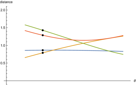
Figure 13: Computing the distance in the plane of a point $q\in S_{p}^{\delta}$ to an arc $q^{\prime}(\theta)$ of the circle $S_{p^{\prime}}^{\delta}$ in $\cal F$, as well as to several copies $q_{i}^{\prime}(\theta)$ of the arc in a neighbourhood of $\cal F$. Each coloured curve segment of distance measurements in the graph on the right corresponds to a different reflection of the arc through one of the vertices.

We show first how to measure the distance between a fixed point $q\!\in\!S_{p}^{\delta}$ and the second circle $S_{p^{\prime}}^{\delta}$. The latter consists of a set of smooth arcs $q^{\prime}(\theta^{\prime})$, not necessarily contained in $\cal F$. For sufficiently small $\delta$, and when $S_{p^{\prime}}^{\delta}$ does not enclose any singularities, there may be just a single “arc”, given by an entire smooth circle and parametrized by $\theta^{\prime}\!\in\![0,2\pi]$. In general there will be several arcs, parametrized by smaller angle intervals. Whatever the case may be, we determine the distance between $q$ and each such arc separately as follows. Consider a specific arc parametrized by $q^{\prime}(\theta^{\prime})\!\in\![\theta^{\prime}_{i},\theta^{\prime}_{f}]$. It is straightforward to determine its distance from $q$ as a function of $\theta^{\prime}$, using the Euclidean distance in the plane. However, recall from our considerations at the beginning of Sec. 5.1 that the corresponding geodesic (straight line) between $q$ and any specific point $q^{\prime}(\theta^{\prime})$ along the arc need not be the shortest one between the corresponding points on the tetrahedron. To find the shortest geodesic in a systematic way, we repeat the distance measurements with each copy (representative) $q^{\prime}_{i}(\theta^{\prime})$ of the arc in the neighbourhood around $\cal F$.

Fig. 13 shows an example where we have collected the distance measurements from four copies of an arc and plotted the corresponding curve segments as a function of $\theta^{\prime}\!\in\![\theta^{\prime}_{i},\theta^{\prime}_{f}]$. The next step is to determine the continuous curve segment that to each $\theta^{\prime}$ in this interval assigns the minimum distance from $q$ to one of the four points $\{q_{1}^{\prime}(\theta^{\prime}),\dots,q_{4}^{\prime}(\theta^{\prime})\}$. This may be a single curve segment, which throughout the $\theta^{\prime}$-interval lies below all other curve segments. Alternatively, it may consist of contributions from several mutually intersecting segments.

The same construction must be applied to the remaining smooth arcs along $S_{p^{\prime}}^{\delta}$. Putting the individual minimizing curve segments together results in a single continuous distance-minimizing curve. Integrating it over $S_{p^{\prime}}^{\delta}$, and dividing it by the length of $S_{p^{\prime}}^{\delta}$ gives the average distance of $q$ to $S_{p^{\prime}}^{\delta}$.

To complete the computation of the average sphere distance (1), we still need to vary the point $q$ over the arcs of the first circle, $S_{p}^{\delta}$. The analysis mirrors the one we just performed for the second circle. It produces a two-dimensional version of the distance-minimizing curve, namely, a distance-minimizing “sheet” parametrized by two angles $(\theta,\theta^{\prime})$, obtained by computing and comparing distances $d(q(\theta),q^{\prime}(\theta^{\prime}))$ between all pairs of points from each pair of arcs from $S_{p}^{\delta}$ and $S_{p^{\prime}}^{\delta}$ respectively, and their representatives in neighbouring domains. These contributions must be combined, integrated and normalized to yield a single data point $\bar{d}(S_{p}^{\delta},S_{p^{\prime}}^{\delta})$ at radius $\delta$.

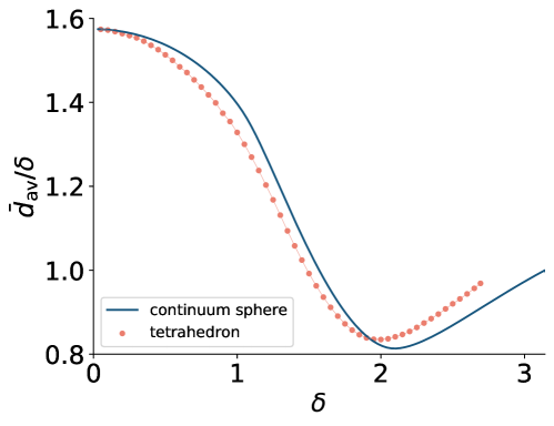
Figure 14: Measurement of the curvature profile $\bar{d}_{\rm av}(\delta)/\delta$ of the surface of a tetrahedron, compared to that of a sphere of the same area. (Error bars too small to be shown.)

To collect the data for the curvature profile, we follow the same procedure as in Sec. 4 to generate double-sphere configurations that are distributed uniformly at random over the tetrahedron. We took random samples of 10.000 average sphere distance measurements at each of 54 evenly spaced values of $\delta$. For easier comparison with the results obtained for the Platonic solids with our earlier method (Fig. 6), we have reverted to “volume-normalized” units where the edge length of the tetrahedron is given by $L\!=\!2.694$ (cf. Table 1). In these units, the step size for measurements is $\delta\!=\!0.05$. The final result for the curvature profile $\bar{d}_{\rm av}(\delta)/\delta$ is shown in Fig. 14, with the curvature profile of the smooth two-sphere for comparison. For small $\delta$, the data are compatible with those obtained with our earlier method.

Overall, the curvature profile of the tetrahedron is qualitatively similar to that of the sphere, but clearly distinct from it, in a way that cannot be absorbed by a simple linear rescaling of the $\delta$-axis. The similarity demonstrates in explicit terms the robustness of this global observable, by which we mean its property of “averaging out” a rather extreme curvature distribution, like that of the tetrahedron. It strengthens earlier observations of such a behaviour on large Delaunay triangulations of a sphere [11]. These are also examples of piecewise flat spaces, but with a curvature distribution that is much closer to that of a continuum sphere, with small deficit angles everywhere.

As the measurements of Sec. 4 already indicated, the curve for $\bar{d}_{\rm av}/\delta$ falls more steeply for small $\delta$, which means that the (averaged) quasi-local quantum Ricci curvature of the tetrahedron is larger than that of the sphere. Features of the sphere curve for larger values $\delta\!\gtrsim\!0.5$ account for large-scale geometric and topological properties of the sphere and are reflected in a similar behaviour of the tetrahedron, although the minimum of the curve is reached for smaller $\delta$ and its value is larger. When interpreting the large-scale behaviour, one should keep in mind that on the two-sphere the circles $S_{p}^{\delta}$ have maximal size for $\delta\!=\!\pi/2$, after which they start shrinking until for $\delta\!=\!\pi$ they degenerate into points. The latter is reflected in the value $\bar{d}_{\rm av}(\pi)/\pi\!=\!1$ on the sphere, the endpoint of the curve in Fig. 14. The fact that each point $p$ on the sphere has an antipode at geodesic distance $\pi$ is of course a consequence of the highly symmetric character of its geometry. As we have already seen, this is different on the tetrahedron, where the distance of the antipode depends on the point $p$ and there is no analogue of the distinguished value $\delta\!=\!\pi$. The restriction on the $\delta$-range we set for the tetrahedron was precisely the distance of the closest antipode. We could in principle have chosen to go beyond this point, assigning the value zero to data points whose antipodal distance is smaller than a given $\delta$. This would have extended the tetrahedron’s curve to $\delta\!\approx\!3.110$, but at the expense of a somewhat unclear interpretation.

6 Summary and conclusion

Motivated by the issue of observables in nonperturbative quantum gravity, we have advocated the study of a new, global geometric observable for curved metric spaces, the curvature profile. It is obtained by integrating the quasi-local, scale-dependent quantum Ricci curvature introduced in earlier work, and has the interpretation of an averaged Ricci scalar depending on a scale $\delta$. On smooth classical manifolds, the information contained in the curvature profile for infinitesimal and small $\delta$ is simply that of the averaged Ricci scalar, while for larger $\delta$ it captures the geometric and topological properties of the metric space in a coarse-grained manner. This scale dependence is very important for the corresponding observable in the quantum theory, where it can help us to identify the transition from a pure quantum regime to a semiclassical one. In order to be able to identify the latter, it is important to get a better understanding of the behaviour of the curvature profile on classical spaces.

In the present work, we have specifically examined the influence of the distribution of the local curvature of the underlying metric space on the classical curvature profile. The easiest set-up to compute and compare this effect explicitly is that of two-dimensional compact surfaces. We have investigated several regular polyhedral surfaces homeomorphic to the two-sphere, which contain a number of conical singularities. We were able to analyze the case of the tetrahedron completely, because we could set up a relatively simple method to compute the geodesic distance between two given points, making use of a representation of the geodesics in the tessellated plane. The curvature profile is distinct from that of the sphere, although its overall features are similar. Perhaps the most remarkable feature is how well it resembles the profile of a smooth sphere. The property of averaging or coarse-graining well over regions where the curvature is singular is a desirable feature from the point of view of the nonperturbative quantum theory, where the quantum geometry on Planckian scales tends to be extremely singular and ill-defined locally. Of course, the quantum Ricci curvature underlying the construction of the curvature profile was introduced precisely to address and potentially mitigate this issue. For the other Platonic solids we could determine the curvature profile only for small $\delta$, but from the limited evidence it appears that distributing the Gaussian curvature over more vertices leads to profiles that are even closer to that of the sphere.

In conclusion, we have for the first time computed a curvature profile for a curved classical space that is not maximally homogeneous and isotropic. It gives us a first quantitative gauge of how deviations from a maximally symmetric situation are reflected in the curvature profile, which constitutes a kind of global fingerprint of a given geometry. It will be interesting to add the curvature profiles of other classical geometries to our reference catalogue, to help us bridge the divide between results from nonperturbative quantum gravity and invariant properties of classical spacetimes.

Acknowledgments. This work was partly supported by a Projectruimte grant of the Foundation for Fundamental Research on Matter (FOM, now defunct), financially supported by the Netherlands Organisation for Scientific Research (NWO).

References

- [1] R. Loll, Discrete approaches to quantum gravity in four dimensions, Living Rev. Rel. 1 (1998) 13 [arXiv:gr-qc/9805049].
- [2] J. Ambjørn, A. Görlich, J. Jurkiewicz and R. Loll, Nonperturbative quantum gravity, Phys. Rep. 519 (2012) 127-210 [arXiv:1203.3591, hep-th].
- [3] R. Loll, Quantum gravity from Causal Dynamical Triangulations: A review, Class. Quant. Grav. 37 (2020) 013002 [arXiv:1905.08669, hep-th].
- [4] J. Ambjørn, Z. Drogosz, J. Gizbert-Studnicki, A. Görlich and J. Jurkiewicz, Pseudo-Cartesian coordinates in a model of Causal Dynamical Triangulations, Nucl. Phys. B (2019) 114626 [arXiv:1812.10671, hep-th].
- [5] J. Ambjørn, J. Jurkiewicz and R. Loll, Emergence of a 4D world from causal quantum gravity, Phys. Rev. Lett. 93 (2004) 131301 [arXiv: hep-th/0404156].
- [6] J. Ambjørn, J. Jurkiewicz and R. Loll, Semiclassical universe from first principles, Phys. Lett. B 607 (2005) 205-213 [arXiv:hep-th/0411152].
- [7] J. Ambjørn, J. Jurkiewicz and R. Loll, Spectral dimension of the universe, Phys. Rev. Lett. 95 (2005) 171301 [arXiv:hep-th/0505113].
- [8] J. Ambjørn, J. Jurkiewicz and R. Loll, Reconstructing the universe, Phys. Rev. D 72 (2005) 064014 [arXiv:hep-th/0505154].
- [9] J. Ambjørn, A. Görlich, J. Jurkiewicz and R. Loll, Planckian birth of the quantum de Sitter universe, Phys. Rev. Lett. 100 (2008) 091304 [arXiv:0712.2485, hep-th].
- [10] J. Ambjørn, A. Görlich, J. Jurkiewicz and R. Loll, The nonperturbative quantum de Sitter universe, Phys. Rev. D 78 (2008) 063544 [arXiv:0807.4481, hep-th].
- [11] N. Klitgaard and R. Loll, Introducing quantum Ricci curvature, Phys. Rev. D 97 (2018) 046008 [arXiv:1712.08847, hep-th].
- [12] N. Klitgaard and R. Loll, Implementing quantum Ricci curvature, Phys. Rev. D 97 (2018) 106017 [arXiv:1802.10524, hep-th].
- [13] N. Klitgaard and R. Loll, How round is the quantum de Sitter universe?, Eur. Phys. J. C 80 (2020) 10, 990 [arXiv:2006.06263, hep-th].
- [14] Y. Ollivier, Ricci curvature of Markov chains on metric spaces, J. Funct. Anal. 256 (2009) 810-864.
- [15] C.A. Trugenberger, Random holographic “large worlds” with emergent dimensions, Phys. Rev. E 94 (2016) no.5, 052305 [arXiv:1610.05339, cond-mat.stat-mech].
- [16] C.A. Trugenberger, Combinatorial quantum gravity: geometry from random bits, JHEP 1709 (2017) 045 [arXiv:1610.05934, hep-th].
- [17] C. Kelly, C.A. Trugenberger and F. Biancalana, Self-assembly of geometric space from random graphs, Class. Quant. Grav. 36 (2019) 125012 [arXiv:1901.09870, gr-qc].
- [18] C. Kelly, C. Trugenberger and F. Biancalana, Emergence of the circle in a statistical model of random cubic graphs [arXiv:2008.11779, hep-th].
- [19] D. Fuchs and E. Fuchs, Closed geodesics on regular polyhedra, Mosc. Math. J. 7 (2007) 265-279.
- [20] D. Fuchs, Periodic billiard trajectories in regular polygons and closed geodesics on regular polyhedra, Geom. Dedicata 170 (2014) 319?333.
- [21] R. Goldstone, R. Roca and R. Suzzi Valli, Shortest paths on cubes [arXiv:2003.06096, math.HO]