Retirement decision and optimal consumption-investment under addictive habit persistence

Abstract.

This paper studies the retirement decision, optimal investment and consumption strategies under habit persistence for an agent with the opportunity to design the retirement time. The optimization problem is formulated as an interconnected optimal stopping and stochastic control problem (Stopping-Control Problem) in a finite time horizon. The problem contains three state variables: wealth $x$, habit level $h$ and wage rate $w$. We aim to derive the retirement boundary of this “wealth-habit-wage” triplet $(x,h,w)$. The complicated dual relation is proposed and proved to convert the original problem to the dual one. We obtain the retirement boundary of the dual variables based on an obstacle-type free boundary problem. Using dual relation we find the retirement boundary of primal variables and feed-back forms of optimal strategies. We show that if the so-called “de facto wealth” exceeds a critical proportion of wage, it will be optimal for the agent to choose to retire immediately. In numerical applications, we show how “de facto wealth” determines the retirement decisions and optimal strategies. Moreover, we observe discontinuity at retirement boundary: investment proportion always jumps down upon retirement, while consumption may jump up or jump down, depending on the change of marginal utility. We also find that the agent with higher standard of life tends to work longer. JEL Classifications: G11, C61. 2010 Mathematics Subject Classification: 91G10, 93E20, 90B50. Keywords: Retirement decision; Stopping-control problem; Habit persistence; Wealth-habit-wage triplet; Retirement boundary; Dual transformation.

1. Introduction

Retirement decision-making has always been an important topic in research fields like quantitative finance, economics and actuarial sciences. In the scenario of voluntary early retirement, it becomes a trade-off between more labour income and more leisure gains for the agent facing the retirement-decision problem. There are more and more works combining voluntary early retirement, optimal investment and optimal consumption. The agent is faced with two problems coupled together: the optimal stopping problem and the stochastic control problem (Stopping-Control Problem, or StopCP for short). The choice of early retirement has been accounted for many reasons, such as health condition, habit formation, socioeconomic status, financial factors, etc. We study the retirement decision-making problem with voluntary early retirement, under linear habit persistence, and aim to give a quantitative and visualized description for retirement boundaries and optimal strategies for consumption and investment. In other words, we investigate this important problem: how do certain factors, such as wealth, standard of life and wage, influence the retirement decision, consumption and investment choice? Optimal consumption and portfolio problems with early retirement option, which are modeled as StopCP, have attracted much attention in the recent decades. Karatzas and Wang (2000) develop dual theory to handle the interaction in StopCP. The problem is transformed to a pure stopping dual problem and then studied by super harmonic characterization or variational methods. Farhi and Panageas (2007) consider voluntary early retirement model with power utility and “no-borrowing-against-future-labour-income” constraint. Choi, Shim, and Shin (2008) and Dybvig and Liu (2010) consider similar problems with no borrowing constraint. More related works in infinite time horizon with StopCP can refer to Jeanblanc, Lakner, and Kadam (2004), Choi and Koo (2005) and Liang, Peng, and Guo (2014), etc. Some recent works have also considered finite horizon problems. In either case, researchers aim at finding thresholds for wealth (or factors) that push the agent to retire. This topic remains very active recently, see Yang and Koo (2018), Park and Jeon (2019), Yang, Koo, and Shin (2020), Jang, Park, and Zhao (2020), Xu and Zheng (2020), etc. Habit persistence has also been taken into consideration in research of finance and economics for decades, which reflects the belief that the more people have consumed in the past, the more they will expect to consume in the future. It has been applied to resolve equity premium puzzle (Sundaresan (1989), Constantinides (1990) and Campbell and Cochrane (1999)), and to be coupled with asset pricing theory (Abel (1990) and Schroder and Skiadas (2002)). More recently, linear habit persistence has been well studied in optimal investment and consumption problem (Englezos and Karatzas (2009), Yu (2012), Yu (2015) and references therein), as well as the target-based insurance management (He, Liang, and Yuan (2020)). Therefore, it would be interesting to investigate how this persistence influences the retirement decision, consumption and investment. To study the influence, we provide the retirement boundary in terms of state triplet $(x,h,w)$ which represent wealth, habit and wage, respectively. Because we consider a finite mandatory retirement time, the StopCP is formulated in a finite time horizon. There come two main difficulties in our model. On the one hand, we must establish dual relation to eliminate the mixed structure of StopCP, which becomes more challenging when habit persistence and finite mandatory retirement time are considered. This is because the problem we consider is formulated in a finite horizon, and the dual free boundary problem does not admit explicit form. In existing literature concerning infinite horizon problem such as Jeanblanc, Lakner, and Kadam (2004), Choi and Koo (2005), Farhi and Panageas (2007), Choi, Shim, and Shin (2008), Dybvig and Liu (2010), Liang, Peng, and Guo (2014), the derived variational inequalities are expected to have closed-form solutions. Therefore, direct verification procedures are sufficient to resolve those problems, and the proofs of the dual relation are not necessary. To find the dual relation in our problem, we need a novel habit reduction method involving stopping times (see Lemmas 3.8 and 3.4). The dual relation is then established by investigating the continuity of stopping time with respect to the dual state variables. Finally we derive an integral equation representation of the dual retirement boundary. On the other hand, the analysis of dual problem becomes complicated because of the introduction of habit formation and an additional state variable $w$. Unlike Yang and Koo (2018), the dual problem is two dimensional, and a change of measure is applied to reduce the dimension. Moreover, we introduce the habit persistence and the time-dependent leisure preference, rather than a negative linear constant penalty as in Yang and Koo (2018). As such, the derived obstacle-type free boundary problem has an inhomogeneous term which evolves with time (see (4.8)), and we find an approach to bypass the monotonicity in time. Furthermore, in our setting, to apply comparison principles, we need growth estimates, which are accomplished by choosing proper auxiliary functions (see Appendix C). In this paper we resolve aforementioned challenges and make the following contributions to the research of early retirement: First, we establish dual theorem in a more complicated model for general utility. The dual relation is established by investigating the continuity of optimal stopping times with respect to dual state variable, and a novel habit reduction method involving stopping times is proposed and used. Second, for power utility we present the retirement boundaries and optimal strategies by so-called “de facto wealth” and wage level. To the best of our knowledge, we are the first to give retirement boundaries in multi-dimensional problems with habit persistence. Although Chen, Hentschel, and Xu (2018) adopt habit formation in retirement problem, the retirement time is pre-commited and deterministic, and they do not give information about the wealth and habit thresholds of retirement. Third, we find that the amount $x-p^{T}(t)h$, called de facto wealth, has clear economic interpretation and appears as threshold for retirement. It is defined by the nominal wealth the agent holds, minus the wealth that he can not actually utilize. In some existing literature where similar quantity has been defined (see Englezos and Karatzas (2009), Chen, Hentschel, and Xu (2018) and Yang and Yu (2019)), it seems that they do not propose its formal definition and emphasize its economic meaning. Besides, they do not consider retirement decision-making for the agent. Based on the theoretical and numerical results of this paper, we can provide an answer to the following important questions: how much wealth is enough for the agent to choose early retirement, and how does this critical wealth level change with different standard of life? The results in this paper indicate that they can be (at least partially) answered by investigating de facto wealth $x-p^{T}(t)h$, which is allowed to be negative (see Remark 3). We prove that if it is far too low, say $x-p^{T}(t)h\leq-q(t)w$, the admissible set is empty. The case $x-p^{T}(t)h>0$ means that he actually has some wealth that he can use freely, and this must be satisfied once he retires (cf. Yu (2015), Yang and Yu (2019)). The retirement boundary is expressed by a linear relation among wealth, habit and wage, which evolves with time. If $x-p^{T}(t)h$ is large enough, that is, $x-p^{T}(t)h\geq G^{*}(t)w$, it is optimal for him to retire (see Proposition 5.4). In addition, we find that, the introduction of habit formation will enlarge the working region of the agent, which is to say, one may work longer than usual if habit is considered. Moreover, the more he is influenced by his habit, the longer time he may choose to work. The numerical results show that the “retirement consumption puzzle” and the “saving for retirement” are implicated in our financial model. The rest of this paper is organized as follows. In Section 2 we set up the model and characterize the admissible set of strategies as well as the allowed region of the state variables, and describe our main problem. Section 3 establishes the dual theorem in a general setting. In Section 4 we present a specific example, and rigorous results about dual retirement boundary are obtained. In Section 5 we obtain the results of retirement boundary in primal coordinate axis and provide a semi-explicit form of optimal consumption and portfolio. Section 6 concludes the paper. Detailed proofs are in the appendices.

2. The Financial Model and Optimization Problem

2.1. The financial market and labour income

Consider a complete filtered probability space $(\Omega,\mathcal{F},\mathbb{F},\mathbb{P})$, where the filtration $\mathbb{F}=\{\mathcal{F}_{t}\}_{0\leq t\leq T}$ satisfies usual conditions with $\mathcal{F}_{T}=\mathcal{F}$. $T<\infty$ is the maximal surviving time from the initial time $t=0$, and $[0,T]$ is the time horizon within which the agent can adjust the strategies.

We suppose that the financial market contains one risk-free asset (bond) $S_{0}=\{S_{0}(t):0\leq t\leq T\}$ and one risky asset (stock) $S_{1}=\{S_{1}(t):0\leq t\leq T\}$. For simplicity, we assume that the prices of these two assets are formulated in the Black-Sholes financial market

$$\mathrm{d}S_{0}(t)=rS_{0}(t)\mathrm{d}t,\quad S_{0}(0)=s_{0},$$

$$\mathrm{d}S_{1}(t)=\mu S_{1}(t)\mathrm{d}t+\sigma S_{1}(t)\mathrm{d}B(t),\quad S_{1}(0)=s_{1},$$

where $r$, $\mu$, $\sigma$, $s_{0}$ and $s_{1}$ are all positive constants. $B=\{B(t):0\leq t\leq T\}$ is a standard Brownian motion on $(\Omega,\mathcal{F},\mathbb{F},\mathbb{P})$ representing market risk. The financial market is complete and we define as usual the exponential martingale and the pricing density $\xi=\{\xi(t):0\leq t\leq T\}$ by

$$Z(t)\triangleq\exp\{-\kappa B(t)-\frac{1}{2}\kappa^{2}t\},$$

$$\xi(t)\triangleq\frac{Z(t)}{S_{0}(t)}=\exp\{-\kappa B(t)-(\frac{1}{2}\kappa^{2}+r)t\},$$

where $\kappa=\frac{\mu-r}{\sigma}$ is the market price of risk. The risk-neutral measure in the financial market is given by $\mathbb{Q}$ with $\frac{\mathrm{d}\mathbb{Q}}{\mathrm{d}\mathbb{P}}\big{|}_{\mathcal{F}_{T}}=Z(T)$. Based on Girsanov’s Theorem, $B_{0}=\{B_{0}(t)=B(t)+\kappa t:\ t\in[0,T]\}$ is a standard Brownian motion on $(\Omega,\mathcal{F},\mathbb{F},\mathbb{Q})$.

The agent invests in the financial market with a continuous stochastic labour income before retirement. We follow Chen, Hentschel, and Xu (2018) to introduce the model of the labour income. The wage rate is assumed to be a geometric Brownian motion with risk perfectly correlated to the financial market. The closed form of the wage rate $\mathcal{W}=\{\mathcal{W}(t):0\leq t\leq T\}$ is

$$\mathcal{W}(t)\triangleq e^{(\mu_{w}-\frac{1}{2}\sigma_{w}^{2})t+\sigma_{w}B(t)},$$

where $\mu_{w}$ and $\sigma_{w}$ are positive constants representing increasing rate and volatility, respectively. Throughout this paper, we consider $\mathcal{W}^{t,w}(\cdot)=w\mathcal{W}(\cdot)/\mathcal{W}(t)$ for some wage rate at present $w>0$. For the agent, there is a mandatory retirement time $T_{1}\in[0,T]$. We assume that the agent has an opportunity to choose the retirement time $\tau\in[0,T_{1}]$. After retirement, the agent has no labour income while more leisure gains. The present value of the future labour income is given by

$$b(s)=\frac{1}{\xi(s)}\mathbb{E}_{s}[\int_{s}^{T_{1}}\xi(u)\mathcal{W}^{t,w}(u)\mathrm{d}u]=\mathcal{W}^{t,w}(s)q(s),\ \ t\in[s,T_{1}].$$ (2.1)

The expectation operator is defined by $\mathbb{E}_{t}(\cdot)=\mathbb{E}[\cdot|\mathcal{F}_{t}]$ and $q(\cdot)$ is a deterministic function. In Dybvig and Liu (2010), Dybvig and Liu (2011), Chen, Hentschel, and Xu (2018) and references therein, a similar $b$ is defined, while in some papers it is defined by the total discounted human capital up to $\tau$, not $T_{1}$. We note that in Choi, Shim, and Shin (2008) and Farhi and Panageas (2007), under the constant wage rate model, it has the form $\frac{w\bar{l}}{r}$. In Yang and Koo (2018), it is $g(s)=-\frac{\rho}{r}(e^{rs-rT_{1}}-1)I_{\{s<T_{1}\}}$ with the constant wage rate $\rho$. In particular, we have $b(t)=q(t)w$, and $q(\cdot)$ can be expressed explicitly

$$q(s)=\left\{\begin{aligned} &\frac{e^{\vartheta(T_{1}-s)}-1}{\vartheta},\vartheta\neq 0,\\ &T_{1}-s,\vartheta=0,\end{aligned}\right.$$ (2.2)

with $\vartheta\triangleq-r+\mu_{w}-\kappa\sigma_{w}$. For theoretical reasons, we assume that

Assumption 1.

$\vartheta<0.$

This assumption requires that $\frac{\mu_{w}-r}{\sigma_{w}}<\kappa$, i.e., the wage rate can not possess log-increase rate too much. Intuitively, the agent may choose to work the whole life in the case of high increasing rate of wage. Then $\tau=T_{1}$, and the problem is a standard stochastic control problem, which is well-studied. Dybvig and Liu (2011) also introduce the same requirement.

2.2. The admissible set of consumption, investment and retirement decision

The agent chooses the retirement time within $[0,T_{1}]$, and we define

$$\mathbb{S}_{t}^{T_{1}}\triangleq\{\tau:\tau\ \mathrm{is}\ \mathrm{an}\ \mathbb{F}-\mathrm{stopping}\ \mathrm{time},\ \mathrm{and}\ t\leq\tau\leq T_{1}\ \mathrm{almost}\ \mathrm{surely}\}.$$

At time $t$, the agent we study will choose a stopping time $\tau\in\mathbb{S}_{t}^{T_{1}}$ as retirement time before the mandatory retirement time $T_{1}<T$. The agent is faced with an optimal portfolio problem after retirement decision is made. The agent will invest in the financial market and consume to satisfy own needs within $[0,T]$. When the consumption rate $c=\{c(s):t\leq s\leq T\}$ and the wealth allocated to risky asset $\pi=\{\pi(s):t\leq s\leq T\}$ are determined, the wealth process satisfies the following stochastic differential equation (abbr. SDE):

$$\left\{\begin{aligned} &\mathrm{d}X(s)=(rX(s)+\pi(s)(\mu-r))\mathrm{d}s-c(s)\mathrm{d}s+\mathcal{W}(s)I_{\{0\leq s\leq\tau\}}\mathrm{d}s+\sigma\pi(s)\mathrm{d}B(s),\\ &X(t)=x.\end{aligned}\right.$$ (2.3)

The agent expects to maintain the standard of living during the working and retirement periods, and has habit persistence. We formulate the standard of living, or the consumption habit level, as the weighted average of the consumption in the past time, plus a decaying term. To be precise, we define the habit level $h^{t,c,h}$ for $t\in[0,T]$ and $h>0$ as

$$\left\{\begin{aligned} &\mathrm{d}h^{t,c,h}(s)=(\alpha c(s)-\beta h^{t,c,h}(s))\mathrm{d}s,\\ &h^{t,c,h}(t)=h,\end{aligned}\right.$$ (2.4)

where $\alpha$ and $\beta$ are positive constants. The goal of the agent is to determine the optimal investment and consumption strategies and the retirement time. The strategies are restricted in the admissible set $\mathcal{A}(t,x,h,w)$ for $(t,x,h,w)\in[0,T_{1}]\times\mathbb{R}\times\mathbb{R}_{+}^{2}$ defined below. Throughout this paper, whenever there is no confusion, we will drop all the superscripts.

Definition 2.1.

For fixed $(t,x,h,w)\in[0,T]\times\mathbb{R}\times\mathbb{R}_{+}^{2}$, $(\tau,c,\pi)\in\mathcal{A}(t,x,h,w)$ if and only if

1. $\tau\in\mathbb{S}_{t}^{T_{1}}$.

2. $c$ and $\pi$ are progressively measurable with respect to $\mathbb{F}$.

3. (2.3) has a unique (strong) solution, denoted by $X^{\tau,c,\pi,t,x}$, with $X(s)+b(s)I_{\{s<\tau\}}\geq 0$ for $s\in[t,T]$, where $b$ is defined in (2.1). We do not consider bequest motives and assume that $X(T)=0$.

4. $$X(\tau)-p^{T}(\tau)h(\tau)>0,\ \ \ \rm almost\ surely,$$ (2.5)

   where $p^{T}(\cdot)$ will be defined in (3.8). $p^{T}(\cdot)$ represents cost of subsistence consumption per unit of habit.

5. $$c(s)-h(s)\geq 0,\ \ \ \rm almost\ surely.$$ (2.6)

6. $$\int_{t}^{T}\pi^{2}(s)\mathrm{d}s<\infty,\int_{t}^{T}c(s)\mathrm{d}s<\infty,\ \ \ \rm almost\ surely.$$

Remark 1.

The constraint $X(t)\geq-b(t)I_{\{t<\tau\}}$ means that the agent is allowed to borrow money and hold a negative wealth level, while the amount of money he borrows can not exceed the total value of future labour income. Once the agent retires, he is prohibited from any borrowing.

Remark 2.

In (4) it is required that $X(\tau)-p^{T}(\tau)h(\tau)>0$. Here $p^{T}(\cdot)$ represents the “cost of subsistence consumption per unit of habit”, as stated in Assumption 2.1 of Yang and Yu (2019). We emphasize that in the retirement setup, we use the subscript $T$ or $\tau$ to distinguish whether it is calculated up to the retirement $\tau$, or the terminal time $T$. The requirement $X(\tau)-p^{T}(\tau)h(\tau)>0$ is the necessary condition to ensure the solvability of the control problem after retirement (where there is no wage income and no retirement option). Similar arguments are shown in Lemma B.1 of Yang and Yu (2019), Lemma 3.3 of Yu (2015) and Theorem 5.5 of Englezos and Karatzas (2009). For detailed discussions, refer to Subsection 2.4 and Section 3.

Remark 3.

Our optimal problem contains three variables. By the form of $x-p^{T}(t)h$, the dimension is reduced. Later we will see that in the expressions of value function or strategies, $(x,h)$ is usually united to $x-p^{T}(t)h$. This motivates us to call this variable as “de facto wealth” of the agent. This reveals that, the same amount of wealth may have different de facto value for agent with different standard of life. For example, $2 for people with higher standard of life may have equal value as $1 for people with lower standard of life. (4) requires that de facto wealth must be positive at retirement.

Remark 4.

The requirement in (2.6) is called “addictive” as the consumption is restricted to be always beyond the standard of living, see Yu (2015). Define $\hat{c}\triangleq c-h$. Obviously, $h(\cdot)$ can also be derived from $\hat{c}$

$$\mathrm{d}h(t)=(\alpha\hat{c}(t)+(\alpha-\beta)h(t))\mathrm{d}t.$$ (2.7)

The agent searches the optimal strategies in the admissible set. We define the set of all “addictive consumption” plans, i.e., all $c=\{c(s):t\leq s\leq T\}$ that satisfy (2), (5) and (6), as $\mathcal{U}_{t}^{T}=\mathcal{U}_{t}^{T}(h)$. Also, define the set of $\pi=\{\pi(s):t\leq s\leq T\}$ that satisfy (2) and (6), as $\mathcal{V}_{t}^{T}$.

2.3. Utility functions and preference change

After retirement, the agent loses labour income while achieves more leisure gains. To distinguish the preferences between working and retirement periods, we define the preferences as follows: $U_{i}(t,x),i=1,2$ are strictly concave utility functions of $x$ satisfying the following conditions:

Assumption 2.

1. $\mathbf{dom}U_{i}=[0,T]\times\mathbb{R}_{+}$, and $U_{i}\in C^{1,2}([0,T]\times\mathbb{R}_{+})$.

2. $\partial_{x}U_{i}(t,+\infty)=0$, $\partial_{x}U_{i}(t,0+)=+\infty$, uniformly in $t$.

3. There exist constants $K$, $C>0$ such that

   $$I_{U_{i}}(t,x)\leq C(1+x^{-K}),\ \ \forall x>0,$$ (2.8)

   where $I_{\phi}=(\phi^{\prime})^{-1}$ for any strictly concave function $\phi$ here and throughout this paper.

For convenience, we denote $U(u,v,x)=U_{1}(u,x)I_{\{u\leq v\}}+U_{2}(u,x)I_{\{u>v\}}$. $U_{1}$ represents the utility before retirement, and $U_{2}$ is the utility after retirement. It can be directly verified that most famous and often-studied utility functions satisfy all the assumptions here, including those in the literature listed above. If $U_{1}<U_{2}$, the agent has utility losses after retirement and will choose to retire at the mandatary retirement time $T_{1}$, which will be shown in Section 4.

2.4. The allowed region of state variables

In this paper, we consider a stochastic labour income and habit formation. Therefore, in our system, we have three state variables: current wealth, habit level and labour income. Before presenting and solving our optimization problem, we briefly discuss and define the allowed region of the state triplet $(x,h,w)$. Define

$$\mathcal{G}_{t}\triangleq\{(x,h,w)\in\mathbb{R}\times\mathbb{R}^{2}_{+}:\ \ \mathcal{A}(t,x,h,w)\neq\varnothing\}.$$ (2.9)

$\mathcal{G}_{t}$ is called the allowed region of state variables. For fixed level of wealth $w$, we denote $\mathcal{G}^{w}_{t}=\{(x,h):(x,h,w)\in\mathcal{G}_{t}\}$. After the strategies are chosen, $(X(s),h(s),\mathcal{W}(s))$ should be contained in $\mathcal{G}_{s}$ for $s\geq t$.

We first consider the agent who retires immediately at $t$. Plugging $\tau=t$ into (2.5), we obtain $x-p^{T}(t)h>0$. Thus we define

$$\mathcal{D}_{t}\triangleq\{(x,h):\ \ x>0,h>0,x-p^{T}(t)h>0\}$$ (2.10)

as the set of positive wealth, habit and de facto wealth. $\mathcal{D}_{t}$ is a natural candidate for $\mathcal{G}_{t}^{w}$. However, it is not clear whether $\mathcal{G}_{t}^{w}=\mathcal{D}_{t}$ holds for any $w$. But it is indeed true that $\mathcal{D}_{t}\subset\mathcal{G}^{w}_{t}$ for any $w$, because if $(x,h)\in\mathcal{D}_{t}$ then $\bar{\mathcal{A}}(t,x,h)\neq\varnothing$, where $\bar{\mathcal{A}}(t,x,h)=\{(c,\pi):(t,c,\pi)\in\mathcal{A}(t,x,h,w)\mathrm{\ for\ some\ }w>0\}$ ($\mathcal{A}(t,x,h,w)$ dose not depend on $w>0$ when $\tau=t$ in the definition, cf. Yang and Yu (2019), Yu (2015) and Englezos and Karatzas (2009)). Moreover, we will see in Section 3 that when $(x,h)\in\mathcal{D}_{t}$, the dual relation also holds. If $(x,h)\notin\mathcal{D}_{t}$, we conclude that the agent never considers retiring now as an option and will continue working. As such, if $(x,h)\in\mathcal{G}_{t}^{w}\backslash\mathcal{D}_{t}$, it is in the continuation region (see Section 5 for the definition). In order to characterize the stopping boundary and show when to retire, we only need to investigate the set $(x,h)\in\mathcal{D}_{t}$. Besides, in Remark 5 we will prove that $\mathcal{G}^{w}_{t}$ has an upper bound.

Finally, we formulate the preference of the agent with retirement choice, consumption and investment strategies. The agent needs to search the optimal strategies to maximize the preference of the whole life. The optimization problem of the agent is a combination of optimal stopping problem and stochastic control problem. In order to maintain the standard of life, the agent cares about the consumption over habit.

We define the objective function for the agent as follows: ​​​​​​​​​​​​​​​​​​​​​

$$\!\!\!\!\!\!\!\!\!\!J(t,x,h,w;\tau,c,\pi)\!\triangleq\!\left\{\!\!\begin{aligned} &\mathbb{E}\!\left[\int_{t}^{T}\!e^{-\rho(s-t)}\!U\big{(}s,\tau,c(s)\!\!-\!\!h(s)\big{)}\!\mathrm{d}s\right],\ \mathrm{if}\ \mathbb{E}\!\left[\int_{t}^{T}\!U^{-}\big{(}s,\tau,c(s)\!\!-\!\!h(s)\big{)}\!\mathrm{d}s\right]\!<\!\infty,\\ &-\infty,\ \ \ \ \ \ \mathrm{otherwise},\end{aligned}\right.$$

where ${U}^{-}=\max\{-{U},0\}$. Then the agent primarily wants to solve the following optimization problem:

$$V(t,x,h,w)=\sup_{(\tau,c,\pi)\in\mathcal{A}(t,x,h,w)}J(t,x,h,w;\tau,c,\pi).\\$$ (2.11)

Problem (2.11) contains optimal stopping and stochastic control, which is not easy to be solved. We will first transform Problem (2.11) into a regular form in Section 3. Then we will formulate the dual relation between primal value function and a value function of a pure optimal stopping problem. Value function of the optimal stopping problem will be characterized by an obstacle-type free boundary problem in Section 4. The optimal retirement time will then be given by the first entrance time of a so-called retirement (stopping) region of the state triplet $(x,h,w)$. The dual relation relies on a novel habit reduction method and the continuity of optimal stopping time.

3. Transformation of the Original Problem

Problem (2.11) is not a standard form of an optimal stopping problem. In this section, we transform Problem (2.11) into an equivalent problem without strategies after retirement. We call the equivalent problem a regular form because it is composed of an integrated utility over the horizon $[0,\tau]$ and a distorted terminal utility at $\tau$. Similar regular form has been studied in Karatzas and Wang (2000) without habit and wage. This regular form also has three state variables and two control variables. After establishing the regular form, we first transform the problem with control variables $(c,\pi)$ to an equivalent one with control variable $c$ only by martingale method. Second, the problem contains an objective function depending pathwisely on $c$. We reduce it to an equivalent problem with a control variable $\hat{c}$ and an objective function that only depends on the value of $\hat{c}(t)$ at each time $t\in[0,T]$. Finally, we establish the dual problem, and disentangle it by a variational inequality and a parabolic equation. We see that in dual coordinate system, the derived variational inequality and parabolic equation are both linear.

3.1. Regular form of Problem (2.11)

In order to represent the integrated utility after retirement in a simple form, we first consider an auxiliary problem, which is a standard optimal consumption-portfolio problem with habit formation while without any labour income or retirement choice. Define the following distorted utility function

$$\bar{U}(t,x,h)=\sup_{(c,\pi)\in\bar{\mathcal{A}}(t,x,h)}\mathbb{E}\left[\int_{t}^{T}e^{-\rho(s-t)}U_{2}\big{(}s,c(s)-h(s)\big{)}\mathrm{d}s\right].$$ (3.1)

If there is no voluntary retirement choice (or retirement time is chosen before $t$) and no labour income, Problem (2.11) degenerates to Problem (3.1). Using the distorted function $\bar{U}(t,x,h)$, we transform the original problem into a regular form without strategies after retirement. The following results ensure the equivalence of these two problems and present the connection between $\bar{U}(t,x,h)$ and strategies after retirement. Similar arguments can refer to Park and Jeon (2019), Liang, Peng, and Guo (2014), Choi, Shim, and Shin (2008) and Jeanblanc, Lakner, and Kadam (2004), etc. The proofs are similar to those in the previously mentioned literature, and we omit them.

Theorem 3.1.

Suppose that $(x,h,w)\in\mathcal{D}_{t}\times\mathbb{R}_{+}$, $t\in[0,T_{1}]$. Denote $\bar{U}^{-}=\max\{-\bar{U},0\}$. Then:

1. For any $\tau\in\mathbb{S}_{t}^{T_{1}}$ and $\mathcal{F}_{\tau}$-measurable random variables $B$ and $C$ such that $(B(\omega),C(\omega))\in\mathcal{D}_{\tau(\omega)}$ for almost sure $\omega\in\Omega$ as well as

   $$\mathbb{E}[\bar{U}^{-}(\tau,B,C)]<+\infty,$$

   there exists a strategy $(\tilde{c},\tilde{\pi})\in\mathcal{U}_{t}^{T_{1}}\times\mathcal{V}_{t}^{T_{1}}$ such that the solution $X^{(\tilde{c},\tilde{\pi})}$ of SDE (2.3) with initial condition $X(\tau)=B$ and the solution $h^{\tilde{c}}$ of (2.4) with initial condition $h(\tau)=C$, satisfy

   $$X^{(\tilde{c},\tilde{\pi})}(s)\geq 0,\ \ \forall s\in[\tau,T],$$

   and

   $$\mathbb{E}\left[\int_{\tau}^{T}e^{-\rho(s-t)}U_{2}(s,\tilde{c}(s)-h^{\tilde{c}}(s))\mathrm{d}s\right]=\mathbb{E}\left[e^{-\rho(\tau-t)}\bar{U}(\tau,B,C)\right].$$ (3.2)

2. For $V$ defined in Problem (2.11), we have

   $$\ \ V(t,x,h,w)$$ (3.3)

   $$\ \ \ \ \ =\!\sup_{(\tau,c,\pi)\in\mathcal{A}(t,x,h,w)}\!\mathbb{E}\left[\int_{t}^{\tau}e^{-\rho(s-t)}U_{1}(s,c(s)\!-\!h(s))\mathrm{d}s\!+\!e^{-\rho(\tau-t)}\bar{U}(\tau,X(\tau),h(\tau))\right].$$

Eq. (3.2) establishes the connection between the utility function $\bar{U}(t,x,h)$ and strategies after retirement. It has an intuitive interpretation that the agent regards the preference after retirement as a standard stochastic control problem because of Markovian property. (LABEL:primalproregular) shows that the original problem is equivalent to the regular form as in Karatzas and Wang (2000). Problem (2.11) with retirement choice and strategies in the whole life is equivalent to the optimization problem with retirement choice, strategies before retirement and claims at retirement. By (3.2), the claims at retirement are correlated with strategies after retirement. We obtain a regular form here, but the optimization problem is still very complex compared to Karatzas and Wang (2000). There exist three state variables $(x,h,w)$ here and the involvement of the habit also brings in difficulties. Next, using habit reduction method and dual method, we solve Problem (LABEL:primalproregular) to derive the strategies for the agent.

3.2. The budget constraints and replication

Before applying dual method, we present the budget constraints in our financial system. We first define the processes $\xi^{t}(\cdot)\triangleq\xi(\cdot)/\xi(t)$ and $S_{0}^{t}(s)\triangleq S_{0}(s)/S_{0}(t)$. In order to transform the original problem with two control variables $(c,\pi)$ into an equivalent one with only one control variable $c$, we consider the set

$$\mathcal{B}(t,x,h,w)\triangleq\{(\tau,c):\ \ \exists\ \pi\mathrm{\ \ s.t.\ \ }(\tau,c,\pi)\in\mathcal{A}(t,x,h,w)\}.$$

For simplicity, we drop the index $(t,x,h,w)$ and write $\mathcal{B}=\mathcal{B}(t,x,h,w)$ if there is no confusion. Based on standard local martingale argument together with optional stopping theorem ( cf. Karatzas and Wang (2000)), we get the following budget constraint:

$$\mathbb{E}\big{[}\underbracket{\xi^{t}(\tau)B}_{\rm wealth\ left\ at\ retirement}+\underbracket{\int_{t}^{\tau}c(u)\xi^{t}(u)\mathrm{d}u}_{\rm wealth\ to\ consume}\big{]}\leq\underbracket{x}_{\rm current\ wealth}+\underbracket{b(t)}_{\rm future\ labour\ income},$$ (3.4)

where $B=X(\tau)+b(\tau)$. Conversely, for any $(\tau,c)\in\mathbb{S}_{t}^{T_{1}}\times\mathcal{U}_{t}^{T}$ (for definition of $\mathcal{U}_{t}^{T}$, see Remark 4) and $\mathcal{F}_{\tau}$-measurable random variable $B>b(\tau)+p^{T}(\tau)h(\tau)$ a.s., such that

$$\mathbb{E}\left[\xi^{t}(\tau)B+\int_{t}^{\tau}c(u)\xi^{t}(u)\mathrm{d}s\right]=x+b(t),$$ (3.5)

we can find some $\pi$ such that the triple $(\tau,c,\pi)\in\mathcal{A}$ based on replication. We introduce the following notations

$$\mathcal{B}_{\leq}\triangleq\{(\tau,c)\in\mathbb{S}_{t}^{T_{1}}\times\mathcal{U}_{t}^{T}:\quad {\rm There\ exists\ \mathcal{F}_{\tau}\ measurable,\ nonnegative\ random\ variable}$$

$$B>b(\tau)+p^{T}(\tau)h(\tau){\rm\ a.s.},{\rm\ such\ that\ (\ref{leqc})\ holds}\},$$

$$\mathcal{B}_{=}\triangleq\{(\tau,c)\in\mathbb{S}_{t}^{T_{1}}\times\mathcal{U}_{t}^{T}:\quad {\rm There\ exists\ \mathcal{F}_{\tau}\ measurable,\ nonnegative\ random\ variable}$$

$$B>b(\tau)+p^{T}(\tau)h(\tau){\rm\ a.s.},{\rm\ such\ that\ (\ref{eqc})\ holds}\}.$$

Then we have the following proposition, which shows the relationship between these three sets:

Proposition 3.2.

$$\mathcal{B}_{=}\subset\mathcal{B}\subset\mathcal{B}_{\leq}.$$

Besides, for any $(\tau,c)\in\mathcal{B}_{=}$, there exists a strategy $\pi$ such that $(\tau,c,\pi)\in\mathcal{A}$ and

$$X(s)+b(s)=\frac{1}{\xi^{t}(s)}\mathbb{E}_{s}[\xi^{t}(\tau)B+\int_{s}^{\tau}\xi^{t}(u)c(u)\mathrm{d}u].$$ (3.6)

Proof.

It is straightforward and similar to the proof of Lemma 6.3 of Karatzas and Wang (2000) with minor modifications, hence omitted. ∎

Proposition 3.6 shows that we only need to search the optimal $(\tau,c)$ first. The optimal investment strategy can be derived by replication. As noted in the expression of budget constraint, $\mathcal{B}_{\leq}$ is the set of all admissible consumption plans whose discounted value does not exceed the total wealth (cash wealth $x$ plus future labour income $b(t)$) of the agent).

3.3. Habit reduction method

To characterize the standard of life, habit persistence is introduced as (2.4), which increases the dimension of our financial system. The preference of the agent also depends on the past consumption path. By the relation of $c$ and $\hat{c}$, we can reduce the original problem to one without habit formation and the path-dependent property. For this habit reduction framework, see Schroder and Skiadas (2002), Englezos and Karatzas (2009), Chen, Hentschel, and Xu (2018) and references therein. The core of such transformation is the relationship between $c$ and $\mathscr{H}c\triangleq\hat{c}=c-h$. The following lemma presents the relationship with the stopping time $\tau$ considered.

Lemma 3.3.

For any $(\tau,c)\in\mathbb{S}_{t}^{T_{1}}\times\mathcal{U}_{t}^{T}$, and $s\in[t,\tau]$, we have

$$\mathbb{E}_{s}\left[\int_{s}^{\tau}c(u)\xi^{t}(u)\mathrm{d}u\right]=\mathbb{E}_{s}\left[\int_{s}^{\tau}\hat{c}(u)\hat{\xi}^{\tau,t}(u)\mathrm{d}u\right]+h(s)\xi^{t}(s)p^{\tau}(s),$$ (3.7)

where

$$\begin{cases}&m(s)=e^{(\alpha-\beta)s},\\ &p^{\tau}(s)=\mathbb{E}_{s}\left[\int_{s}^{\tau}\frac{m(u)}{m(s)}\frac{\xi^{t}(u)}{\xi^{t}(s)}\mathrm{d}u\right],\\ &\mu^{\tau}(s)=1+\alpha p^{\tau}(s),\\ &\hat{\xi}^{t,\tau}(s)=\xi^{t}(s)+\alpha\mathbb{E}_{s}\left[\int_{s}^{\tau}\frac{m(u)}{m(s)}\xi^{t}(u)\mathrm{d}u\right]=\mu^{\tau}(s)\xi^{t}(s).\end{cases}$$ (3.8)

Proof.

See Appendix A. ∎

Lemma 3.8 shows that the integrand in the budget constraint of (3.4) can be replaced by $\hat{c}$. As the agent only cares about the consumption over habit, i.e., $\hat{c}=c-h$, we can reduce the problem to one with control $\hat{c}$ while without habit $h$. In particular, if we choose $(\tau,c)\in\mathcal{B}_{\leq}$ and take $s=t$ in (3.7), the budget constraint (3.4) becomes

$$\mathbb{E}\left[\underbracket{\xi^{t}(\tau)(X(\tau)+b(\tau))}_{\rm wealth\ left\ at\ retirement}+\underbracket{\int_{t}^{\tau}\hat{c}(u)\mu^{\tau}(u)\xi^{t}(u)\mathrm{d}u}_{\rm wealth\ to\ consume}\right] +\underbracket{hp^{\tau}(t)}_{\rm wealth\ needed\ to\ satisfy\ habit}$$ (3.9)

$$\leq\underbracket{x}_{\rm current\ wealth} +\underbracket{b(t)}_{\rm future\ labour\ income}.$$

We now transform our problem into an equivalent one w.r.t. control $\hat{c}$. Define the mapping $\mathscr{H}:c\mapsto\hat{c}$ and the set $\hat{\mathcal{U}}_{t}^{T}\triangleq\mathscr{H}\mathcal{U}_{t}^{T}$. First, we define $\hat{\mathcal{B}}_{\leq}$ as the set of all $(\tau,\hat{c})\in\mathbb{S}_{t}^{T_{1}}\times\hat{\mathcal{U}}_{t}^{T}$ satisfying (3.9), with $X(\tau)+b(\tau)$ replaced by some $\mathcal{F}_{\tau}$ measurable random variable $B\geq b(\tau)+p^{T}(\tau)h(\tau)$ a.s., and define $\hat{\mathcal{B}}_{=}$ as those $(\tau,c)$ satisfying the equality in (3.9). Then we have the natural inclusions

$$\hat{\mathcal{B}}_{=}=\tilde{\mathscr{H}}\mathcal{B}_{=}\subset\tilde{\mathscr{H}}\mathcal{B}\subset\tilde{\mathscr{H}}\mathcal{B}_{\leq}\subset\hat{\mathcal{B}}_{\leq},$$

where the mappings $\mathscr{H}:c\mapsto\hat{c}$ and $\tilde{\mathscr{H}}:(\tau,c)\mapsto(\tau,\hat{c}=\mathscr{H}c)$ are both linear. We see that it has a natural inverse map $\mathscr{H}^{-1}:\hat{c}\mapsto c$. In Lemma 3.8, when replacing $c$ by $\hat{c}$, we have an additional multiplier $\mu^{\tau}$ and an additional term $p^{\tau}$. Because these two additional terms both depend on $\tau$, the dual problem is hard to be derived and solved. In order to establish the dual problem, we need to calculate these terms in more concrete forms. We have the following lemma.

Lemma 3.4.

Denote $\hat{\mathcal{U}}_{t}^{T_{1}}\triangleq\mathscr{H}\mathcal{U}_{t}^{T_{1}}$. For any $(\tau,\hat{c})\in\mathbb{S}_{t}^{T_{1}}\times\hat{\mathcal{U}}_{t}^{T_{1}}$, and $s\in[t,\tau]$ we have

$$\mathbb{E}_{s}\left[\int_{s}^{\tau}\xi^{t}(u)\mu^{\tau}(u)\hat{c}(u)\mathrm{d}u+h(s)p^{\tau}(s)\right] =\mathbb{E}_{s}\left[\int_{s}^{\tau}\xi^{t}(u)\mu^{T}(u)\hat{c}(u)\mathrm{d}u-h(\tau)\xi^{t}(\tau)p^{T}(\tau)\right]$$ (3.10)

$$\ \ \ \ +\mathbb{E}_{s}\left[\xi^{t}(s)h(s)p^{T}(s)\right],$$

where $\mu^{T}$ and $p^{T}$ are defined as in Lemma 3.8 with $\tau$ replaced by $T$, respectively.

Proof.

See Appendix A. ∎

Remark 5.

We can present an upper bound for the allowed region $\mathcal{G}_{t}$ as follows. For definition of $\mathcal{G}_{t}$, refer to (2.9). Define

$$\mathcal{E}_{t}=\{(x,h,w):\ \ x-p^{T}(t)h+q(t)w>0\},$$ (3.11)

$$\mathcal{E}_{t}^{w}=\{(x,h):\ \ (x,h,w)\in\mathcal{E}_{t}\}.$$ (3.12)

We claim that $\mathcal{G}_{t}\subset\mathcal{E}_{t}$. In fact, combining (3.9) and (3.10), we know that if $(x,h,w)\in\mathcal{G}_{t}$, then

$$x-p^{T}(t)h+q(t)w\geq\mathbb{E}[\xi^{t}(\tau)(X(\tau)-p^{T}(\tau)h(\tau))]>0$$

holds for any $(\tau,c)\in\mathcal{B}(t,x,h,w)\subset\mathcal{B}_{\leq}(t,x,h,w)$. Therefore, $\mathcal{G}_{t}\subset\mathcal{E}_{t}$. From the proof of Theorem 3.5 we know that if some further information of $\hat{\tau}_{y}$ is available, the lower bound of $\mathcal{G}_{t}$ will be tighter. If, in addition, we can prove $\lim_{y\to\infty}\mathbb{E}b(\hat{\tau}_{y})\xi^{t}(\hat{\tau}_{y})=0$, the equality $\mathcal{G}_{t}=\mathcal{E}_{t}$ holds. This upper bound requires that the agent can not let his de facto wealth fall below the negative value of his future labour income.

We have replaced the budget constraint w.r.t. $c$ by $\hat{c}$. The linearity of the budget constraint ensures the existence of the dual problem. The next subsection will be dedicated to solving Problem (LABEL:primalproregular) based on dual approach.

3.4. The dual problem

Problem (LABEL:primalproregular) is still a combination of optimal stopping and stochastic control problems. In order to separate the stopping time and stochastic controls, we first define the dual functions of “running utility” $U_{1}$ and “terminal utility” $\bar{U}$, respectively. By the dual approach, Problem (LABEL:primalproregular) can be transformed to a pure optimal stopping problem (see Park and Jeon (2019), Yang and Koo (2018), Liang, Peng, and Guo (2014), Choi, Shim, and Shin (2008) or Karatzas and Wang (2000) for such a transformation). After obtaining the optimal stopping problem, we construct the corresponding variational inequality. Then we derive the retirement boundary in terms of the dual variables. As such, the relationship between the dual variables and primal variables induces the retirement boundary w.r.t. the primal variables. Moreover, in order to obtain the properties of $\bar{U}$ and its dual function, a parabolic equation will be established. At last, the verification theorem will be stated and proved in Section 4 based on the optimal strategies in the dual variables, and the properties of optimal strategies in the original variables will be listed and proved in Section 5. Define the dual variable $Y^{t,y}(s)=ye^{\rho(s-t)}\xi^{t}(s)$, and observe that for $y>0$, using Lemmas 3.8 and 3.4 we have ​​​​​​​

$$V(t,x,h,w)\!-\!y(x+b(t))$$

$$\leq\sup_{(\tau,\hat{c})\in\hat{\mathcal{B}}_{\leq}}\mathbb{E}\left[e^{-\rho(\tau-t)}\bar{U}(\tau,X(\tau),h(\tau))\!+\!\int_{t}^{\tau}e^{-\rho(u-t)}U(u,\hat{c}(u))\mathrm{d}u\right]$$

$$\ \ \ \ -y\mathbb{E}\left[\xi^{t}(\tau)(X(\tau)\!+\!b(\tau))\!+\!\int_{t}^{\tau}\hat{c}(u)\mu^{\tau}(u)\xi^{t}(u)\mathrm{d}u+hp^{\tau}(t)\right]$$

$$=\sup_{(\tau,\hat{c})\in\hat{\mathcal{B}}_{\leq}}\mathbb{E}\left[e^{-\rho(\tau-t)}\left(\bar{U}(\tau,X(\tau),h(\tau))\!-\!Y^{t,y}(\tau)(X(\tau)\!+\!b(\tau)\!-\!p^{T}(\tau)h(\tau))\right)\right]$$

$$\ \ \ \ +\mathbb{E}\left[\int_{t}^{\tau}e^{-\rho(u-t)}\left(U(u,\hat{c}(u))\!-\!Y^{t,y}(u)\hat{c}(u)\mu^{T}(u)\right)\mathrm{d}u\right]\!-\!hp^{T}(t)$$

$$\leq\!\!\sup_{\tau\in\mathbb{S}_{t}^{T_{1}}}\!\mathbb{E}\!\left[\!e^{-\rho(\tau-t)}\bar{V}(\tau,Y^{t,y}(\tau),w^{t,w}(\tau))\!+\!\int_{t}^{\tau}e^{-\rho(u-t)}\hat{V}_{1}(u,Y^{t,y}(u))\mathrm{d}u\right]\!-\!hp^{T}(t),$$ (3.13)

where

$$\bar{V}(t,y,w) \triangleq \sup_{(x,h)\in\mathcal{D}_{t}}\{\bar{U}(t,x,h)-y(x-p^{T}(t)h)\}-yq(t)w,$$ (3.14)

$$\hat{V}_{1}(t,y) \triangleq \sup_{c>0}\{U_{1}(t,c)-y\mu^{T}(t)c\}.$$ (3.15)

As such, if we introduce the following optimal stopping problem

$$\!\!\!\!W(t,y,w) = \sup_{\tau\in\mathbb{S}_{t}^{T_{1}}}\mathbb{E}\left[e^{-\rho(\tau-t)}\bar{V}(\tau,Y^{t,y}(\tau),w^{t,w}(\tau))\!\!+\!\!\int_{t}^{\tau}e^{-\rho(u-t)}\hat{V}_{1}(u,Y^{t,y}(u))\mathrm{d}u\right]$$ (3.16)

$$= \sup_{\tau\in\mathbb{S}_{t}^{T_{1}}}\mathbb{E}^{t,y,w}\left[e^{-\rho(\tau-t)}\bar{V}(\tau,Y(\tau),\mathcal{W}(\tau))+\int_{t}^{\tau}e^{-\rho(u-t)}\hat{V}_{1}(u,Y(u))\mathrm{d}u\right],$$

we have that $\forall t\in[0,T_{1}],\ (x,h)\in\mathcal{D}_{t},\ y>0$ and $w>0$,

$$V(t,x,h,w)-y(x+q(t)w-p^{T}(t)h)\leq W(t,y,w).$$ (3.17)

Thus, if we establish the relationship between Problem (LABEL:primalproregular) and the dual problem (3.16), the dual problem contains no controls and is a pure optimal stopping problem, which is easier to be solved. In fact, we have the following dual theorem to guarantee the equivalence of these two problems.

Theorem 3.5.

Let $t\in[0,T_{1})$, $w>0$ and $(x,h)\in\mathcal{D}_{t}$ be fixed. Suppose that the optimal stopping time $\hat{\tau}_{y}=\hat{\tau}_{t,y,w}$ of Problem (3.16) can be chosen such that $\hat{\tau}_{y+\varepsilon}\to\hat{\tau}_{y}$ almost surely as $\varepsilon\to 0\pm$, then the value function of Problem (2.11) satisfies

$$V(t,x,h,w)=\inf_{y>0}\{W(t,y,w)+y(x-p^{T}(t)h)+yq(t)w\}.$$ (3.18)

Proof.

See Appendix B. ∎

Theorem 3.5 proposes the framework for dual argument with endogenous habit persistence and general utility. In practice, the conditions are usually verified depending on the form of the problem (see Section 5 for example). Besides, our argument shows that only the continuity of $\hat{\tau}_{y}$ is needed to establish the dual relation, which remains true under some mild regularities of the boundary (see the proof of Lemma 5.1).

3.5. Properties of the post-retirement value function $\bar{U}$

In Problem (LABEL:primalproregular), there exists a utility function $\bar{U}$, which is related to the integral of $U_{2}$ after retirement. We observe in Problem (3.16) that we need to introduce the dual function $\bar{V}$ of the function $\bar{U}$. In order to solve the dual problem, we briefly discuss the properties of $\bar{U}$. We list them in the following several lemmas, of which all proofs are omitted, because they are all classical results and can be found in, e.g., Englezos and Karatzas (2009) or Yu (2015).

Lemma 3.6.

For $t\in[0,T_{1})$ and $(x,h)\in\mathcal{D}_{t}$, we have

$$\bar{U}(t,x,h)=\tilde{U}(t,x-p^{T}(t)h),$$ (3.19)

where $\tilde{U}(t,\cdot)$ is strictly concave for any fixed $t$.

Lemma 3.6 shows that the integrated utility after retirement relies on the de facto wealth $x-p^{T}(t)h$, and the dimension of state space has been essentially reduced by one. We will see that the optimal strategies of the agent depend on $x,h$ through $x-p^{T}(t)h$. By habit reduction method, Problem (3.1) can be transformed to a standard optimal consumption problem without habit formation. As such, we apply the dual approach to solve the standard problem. We have the following lemma of the standard optimal consumption problem.

Lemma 3.7.

Define

$$\tilde{V}(t,y)\triangleq\mathbb{E}\left[\int_{t}^{T}e^{-\rho(u-t)}\hat{V}_{2}(u,Y^{t,y}(u))\mathrm{d}u\right],$$ (3.20)

where

$$\hat{V}_{2}(t,y)=\sup_{c>0}\{U_{2}(t,c)-y\mu^{T}(t)c\}.$$

Then we have the following dual relation:

$$\tilde{V}(t,y)=\sup_{z>0}\{\tilde{U}(t,z)-yz\},$$ (3.21)

$$\tilde{U}(t,z)=\inf_{y>0}\{\tilde{V}(t,y)+yz\}.$$ (3.22)

Lemma 3.7 shows that $\hat{V}_{2}(t,y)$ can be derived by the dual relation with $U_{2}(t,c)$. We rely on the dual relation with $\tilde{V}$ to obtain $\tilde{U}$. However, $\tilde{V}$ is unknown, but (3.20) establishes the relation between $\tilde{V}$ and $\hat{V}_{2}$. Using Feynman-Kac’s formula, we can obtain the following lemma to get $\tilde{V}$ from $\hat{V}_{2}$.

Lemma 3.8.

Let $\mathcal{N}_{T}\triangleq[0,T)\times\mathbb{R}_{+}$ and $\overline{\mathcal{N}}_{T}\triangleq[0,T]\times\mathbb{R}_{+}$. Define

$$\tilde{\mathscr{L}}\triangleq y(\rho-r)\partial_{y}+\frac{1}{2}y^{2}\kappa^{2}\partial_{yy}-\rho.$$

Then we have

1. $\tilde{V}\in C^{1,2}(\mathcal{N}_{T})\cap C(\overline{\mathcal{N}_{T}})$, and

   $$\left\{\begin{aligned} &(-\partial_{t}-\tilde{\mathscr{L}})\tilde{V}=\hat{V}_{2},\mathrm{\ in\ }\mathcal{N}_{T},\\ &\tilde{V}(T,\cdot)=0.\end{aligned}\right.$$ (3.23)

2. For any fixed $t$, $\tilde{V}(t,y)$ is strictly convex and strictly decreasing with respect to $y$. In addition, there exist constants $C$ and $K$ such that

   $$|\partial_{y}\tilde{V}|\leq C(1+y^{-K}),\ \ \forall(t,y)\in\mathcal{N}_{T}.$$ (3.24)

Remark 6.

In fact, from the proof of Lemma 3.8 we know that for any other measure $\tilde{\mathbb{P}}$ and corresponding expectation operator $\tilde{\mathbb{E}}$, if we have the expression

$$\tilde{V}(t,z)\triangleq\tilde{\mathbb{E}}\left[\int_{t}^{T}e^{-\bar{\rho}(u-t)}\hat{V}_{2}(u,Z^{t,z}(u))\mathrm{d}u\right],$$

where $Z$ is any diffusion process with drift term $\mu_{Z}$ and diffusion term $\sigma_{Z}$ under $\tilde{\mathbb{P}}$, then

$$\left\{\begin{aligned} &(-\partial_{t}-\mathscr{L}_{Z})\tilde{V}=\hat{V}_{2},\mathrm{\ in\ }\mathcal{N}_{T},\\ &\tilde{V}(T,\cdot)=0,\end{aligned}\right.$$ (3.25)

with

$$\mathscr{L}_{Z}=z\mu_{z}\partial_{z}+\frac{1}{2}z^{2}\partial_{zz}-\bar{\rho}.$$

Remark 7.

In this section we know that $\bar{V}(t,y,w)=\tilde{V}(t,y)-q(t)yw$ and $\bar{V}$ is strictly convex w.r.t. $y$. Thus, using the same arguments as in Lemma 8.1 of Karatzas and Wang (2000), we can prove that $W$ is strictly convex w.r.t. $y$, which is a necessary condition in Section 5.

4. Retirement Boundary in Terms of Dual Variables

Section 3 presents the theoretical results of the StopCP. In order to obtain the forms of the retirement boundary and optimal strategies, we specify the preferences by the CRRA utility function and a time-dependent leisure model. Our analysis relies highly on the homogeneous structure of the utility function, otherwise the retirement boundary will be rather difficult to describe. Unlike Yang and Koo (2018), the primal problem contains three variables and the dual problem contains two variables. As such, more general analysis with other preferences may be impossible. We consider the following preferences before and after retirement:

$$U_{1}(t,x)=\frac{x^{1-\gamma}}{1-\gamma},$$ (4.1)

$$U_{2}(t,x)=K(t)\frac{x^{1-\gamma}}{1-\gamma},$$ (4.2)

where $\gamma>0$, $\gamma\neq 1$ is the risk aversion of the agent and $K(\cdot)>0$ is a smooth function which represents the leisure preference. As the retiree always has less leisure gains as time goes by, we consider a time dependent leisure preference function here. Especially in the case that $K(t)^{1-\gamma}\leq 1$, i.e., $U_{1}\geq U_{2}$, which means that the agent has leisure losses after retirement, he will never choose to retirement until mandatory retirement time.

4.1. Measure change

To characterize the retirement boundary in dual variables, we need to solve the dual optimal stopping problem (3.16) without controls. However, Problem (3.16) is two dimensional and the infinitesimal operator of Markov process $(Y(\cdot),w(\cdot))$ is degenerate, which bring twofold difficulties. First, establishing the existence, uniqueness and regularity of the associated differential equations and obstacle-type free boundary problems is quite difficult (although there are indeed some classical results in the field of partial differential equations). Second, the retirement boundary naturally depends on the pair $(y,w)$. We can hardly guess and describe the retirement boundary with two state variables. In fact, when there is only one variable, we can simply conjecture that the stopping region has the form $\{z\leq z^{*}(t)\}$ or $\{z\geq z^{*}(t)\}$ (where $z$ is the reduced variable) and then verify it. In order to obtain the retirement boundary, we apply a measure change method to reduce these two state variables $(y,w)$ to one variable.

Lemma 4.1.

Consider the exponential martingale

$$\mathcal{E}=\left\{\mathcal{E}(t)=\exp\left(-\frac{1}{2}(\sigma_{w}-\kappa)^{2}t+(\sigma_{w}-\kappa)B(t)\right):\ \ 0\leq t\leq T_{1}\right\}.$$

Let $\mathrm{d}\tilde{\mathbb{P}}=\mathcal{E}(T_{1})\mathrm{d}\mathbb{P}$ and $\tilde{\mathbb{E}}$ be the corresponding expectation operator. Then we have

$$W(t,y,w)/yw=\tilde{w}(t,z)$$

with

$$\tilde{w}(t,z)=\sup_{\tau\in\mathbb{S}_{t}^{T_{1}}}\tilde{\mathbb{E}}^{t,z}\left[\int_{t}^{\tau}e^{\vartheta(u-t)}\hat{V}_{1}(u,Z(u))\mathrm{d}u+e^{\vartheta(\tau-t)}(\tilde{V}(\tau,Z(\tau))-q(\tau))\right],$$ (4.3)

and the change of variable $z=y^{1/(1-\gamma)}w^{\gamma/(1-\gamma)}$. The underlying Markov process $Z$ is defined by

$$Z=Y^{1/(1-\gamma)}\mathcal{W}^{\gamma/(1-\gamma)}.$$

Proof.

Combining (3.14), (3.19) and (3.21), we have

$$\bar{V}(t,y,w)=\tilde{V}(t,y)-ywq(t).$$

Direct calculations show

$$Y(t)\mathcal{W}(t)=e^{(\rho+\vartheta)t}\mathcal{E}(t).$$

Then the Bayesian rules of the measure change (c.f. Lemma 3.5.3 of Karatzas and Shreve (1991)) imply that for any fixed $\tau\in\mathbb{S}_{t}^{T_{1}}$,

$$\mathbb{E}^{t,y,w} \left[e^{-\rho(\tau-t)}\bar{V}(\tau,Y(\tau),\mathcal{W}(\tau))\right]$$

$$=\mathbb{E}^{t,y,w}\left[e^{-\rho(\tau-t)}Y(\tau)\mathcal{W}(\tau)(\tilde{V}(\tau,Y(\tau))/Y(\tau)\mathcal{W}(\tau)-q(\tau))\right]$$

$$=\mathbb{E}^{t,z}\left[e^{-\rho(\tau-t)+(\rho+\vartheta)\tau}\mathcal{E}(\tau)(\tilde{V}(\tau,Z(\tau))-q(\tau))\right]$$

$$=yw\tilde{\mathbb{E}}^{t,z}\left[e^{\vartheta(\tau-t)}(\tilde{V}(\tau,Z(\tau))-q(\tau))\right],$$

where we have used the homogeneous property

$$\tilde{V}(t,y)/yw=\tilde{V}(t,y(yw)^{-\gamma/(\gamma-1)}).$$

Based on the same arguments, we also have

$$\mathbb{E}^{t,y,w}\left[\int_{t}^{\tau}e^{-\rho(u-t)}\hat{V}_{1}(u,Y(u))\mathrm{d}u\right]=yw\tilde{\mathbb{E}}^{t,z}\left[\int_{t}^{\tau}e^{\vartheta(u-t)}\hat{V}_{1}(u,Z(u))\mathrm{d}u\right].$$

Combining the above calculations, the results are derived. ∎

Lemma 4.1 shows that the dual problem (3.16) with two state variables $(y,w)$ is equivalent to the reduced dual problem (4.3) with one state variable $z=y^{1/(1-\gamma)}w^{\gamma/(1-\gamma)}$. Using optimal stopping theory, we obtain the optimal stopping time of Problem (4.3). We observe in Problem (4.3) that the discount factor is $\vartheta$, which initially appears in (2.2). Based on Assumption 1 we have $\vartheta<0$. It is interesting to further explore this connection.

4.2. The free boundary problem of Problem (4.3)

In this subsection we solve the dual problem (4.3) by deriving the related free boundary problem. We first establish the verification theorem for Problem (4.3), and propose some regularities that will be necessary later. The existence of the solution of the associated free boundary problem can be verified based on the classical theory of free boundary problems. We present two important theorems (Theorems 4.2 and 4.3) in this subsection.

Theorem 4.2.

Denote $\mathcal{N}_{T_{1}}\triangleq[0,T_{1})\times\mathbb{R}_{+}$. Suppose that there exists a function $\hat{w}\in C(\overline{\mathcal{N}_{T_{1}}})\cap C^{1,1}(\mathcal{N}_{T_{1}})\cap C^{1,2}(\mathcal{C})\cap C^{1,2}(\mathcal{N}_{T_{1}}\backslash\overline{\mathcal{C}})$ satisfying the following conditions:

1. $\hat{w}\geq\tilde{V}-q$,

2. The open subset $\mathcal{C}=\{(t,z):\ \hat{w}>\tilde{V}-q\}\subset\mathcal{N}_{T_{1}}$ has a Lipschitz continuous boundary $\partial\mathcal{C}$,

3. $Z(t)$ spends almost no time on $\partial\mathcal{C}$, i.e.,

   $$\int_{t}^{T_{1}}I_{\{(u,Z(u))\in\partial\mathcal{C}\}}\mathrm{d}u=0,\ \ \mathbb{P}^{t,z}-{\rm almost\ surely,\ for\ any\ }(t,z)\in\mathcal{N}_{T_{1}},$$ (4.4)

4. $\hat{w}$ satisfies the growth condition:

   $$|\hat{w}(t,z)|+|\partial_{z}\hat{w}(t,z)|\leq C(z^{K}+z^{-K}),\ \ \forall(t,z)\in\mathcal{N}_{T_{1}},$$ (4.5)

5. $\hat{w}$ solves the following obstacle-type free boundary problem:

   $$\left\{\begin{aligned} &(-\partial_{t}-\mathscr{L}_{Z})\hat{w}=\hat{V}_{1}{\rm\ in\ }\mathcal{C},\\ &(-\partial_{t}-\mathscr{L}_{Z})\hat{w}\geq\hat{V}_{1}{\rm\ in\ }\mathcal{N}_{T_{1}}\backslash\mathcal{C},\\ &\hat{w}(T_{1},\cdot)=\tilde{V}(T_{1},\cdot)-q(T_{1}),\end{aligned}\right.$$ (4.6)

   where

   $$\mathscr{L}_{Z}=\frac{\sigma_{z}^{2}}{2}z^{2}\partial_{zz}+\mu_{z}z\partial_{z}+\vartheta,$$

   with $\mu_{z}$ and $\sigma_{z}$ representing the drift and diffusion coefficients of $Z$, respectively,

we have $\tilde{w}=\hat{w}$ in $\mathcal{N}_{T_{1}}.$

Proof.

See Appendix C ∎

The regularities proposed in Theorem 4.2 are sufficient and necessary. $\hat{w}_{z}(t,z)$ is continuous while not differentiable at $z=z^{*}(t)$, which is illustrated in the numerical example of Figure 1. More details of the parameters and the numerical method can refer to Subsection 4.4.

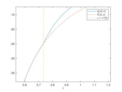
(a) $\gamma=0.5$

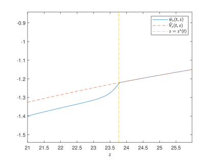
(b) $\gamma=1.5$

Figure 1. $\hat{w}_{z}(t,\cdot)$ and $\tilde{V}_{z}(t,\cdot)$ at time $t=8$.

As $\hat{w}$ is not necessary to have second order derivatives on the boundary $\partial\mathcal{C}$, the inequalities for $\hat{w}$ in (4.6) hold in limit sense, i.e.,

$$(-\partial_{t}-\mathscr{L}_{Z})\hat{w}\geq\hat{V}_{1}{\rm\ in\ }{\rm int}\{\mathcal{N}_{T_{1}}\backslash\partial\mathcal{C}\}$$

implies that

$$\liminf_{\tiny\begin{array}[]{c}(t^{\prime},z^{\prime})\notin\partial\mathcal{C}\\ (t^{\prime},z^{\prime})\to(t,z)\end{array}}\{(-\partial_{t}-\mathscr{L}_{Z})\hat{w}(t^{\prime},z^{\prime})-\hat{V}_{1}(t^{\prime},z^{\prime})\}\geq 0{\rm\ on\ }\partial\mathcal{C}.$$

The following theorem ensures the existence of $\hat{w}$.

Theorem 4.3.

The free boundary problem (4.6) admits a solution that satisfies all the conditions in Theorem 4.2.

Proof.

Using classical theory of free boundary problems (or variational inequalities), we can easily obtain the regularities of $\hat{w}$ and $\partial\mathcal{C}$. The derivation is similar to that Friedman (1975) and we omit it here. In Appendix C, we prove Theorem 4.5 to ensure other properties of $\partial\mathcal{C}$, the growth condition (4.5) and other further results. (4.4) follows naturally from the properties of $\partial\mathcal{C}$ and the regularity of the process $Z$. ∎

Now we solve the free boundary problem and show the optimal retirement time. We mainly concentrate on the regularity property, the growth condition (4.5) and the differential inequality (4.6) of $\tilde{w}$.

4.3. The retirement boundary of Problem (4.3)

In this subsection, we characterize the retirement boundary based on a critical value of the reduced variable $z$. The boundary condition in (4.6) has two functions $\tilde{V}$ and $q(t)$. In order to eliminate these two functions, we define a new function $F(t,z)\triangleq\tilde{w}(t,z)-\tilde{V}(t,z)+q(t)$ and study the stopping region $\mathcal{S}=\{(t,z):F=0\}$ and the continuation region $\mathcal{C}=\{(t,z):F>0\}$. Combining (3.25) and (4.6), $F$ satisfies the following obstacle-type free boundary problem:

$$\left\{\begin{aligned} &(-\partial_{t}-\mathscr{L}_{Z})F=\hat{V}_{1}-\hat{V}_{2}+1{\rm\ in\ }\mathcal{C},\\ &(-\partial_{t}-\mathscr{L}_{Z})F\geq\hat{V}_{1}-\hat{V}_{2}+1{\rm\ in\ }\mathcal{S},\\ &F(T_{1},\cdot)=0.\end{aligned}\right.$$ (4.7)

The right hand side of the above equation can be calculated explicitly

$$\hat{V}_{1}(t,z)-\hat{V}_{2}(t,z) =\frac{1}{\tilde{\gamma}}(\mu^{T}(t)z)^{-\tilde{\gamma}}-\frac{K(t)^{1/\gamma}}{\tilde{\gamma}}(\mu^{T}(t)z)^{-\tilde{\gamma}}$$

$$=\triangle(t)(\mu^{T}(t)z)^{-\tilde{\gamma}},$$

where $\tilde{\gamma}=(1-\gamma)/\gamma$ and $\triangle(t)=\frac{1-K(t)^{1/\gamma}}{\tilde{\gamma}}$. Here we have used the fact $(-\partial_{t}-\mathscr{L}_{Z})q(t)=-q^{\prime}(t)-\vartheta q(t)=1$, which is obvious by the expression (2.2) of $q$. For convenience, we rewrite Problem (4.7) as follows:

$$\left\{\begin{aligned} &(-\partial_{t}-\mathscr{L}_{Z})F=\triangle(t)(\mu^{T}(t)z)^{-\tilde{\gamma}}+1{\rm\ in\ }\mathcal{C},\\ &(-\partial_{t}-\mathscr{L}_{Z})F\geq\triangle(t)(\mu^{T}(t)z)^{-\tilde{\gamma}}+1{\rm\ in\ }\mathcal{S},\\ &F(T_{1},\cdot)=0.\end{aligned}\right.$$ (4.8)

The sign of $\triangle(t)$ is an indicator to show whether the agent has leisure gains or losses. Precisely, $\triangle(t)<0$ is equivalent to $U_{1}<U_{2}$ in our problem. The following proposition shows that if $U_{1}\geq U_{2}$, the agent will never retire, which is quite natural.

Proposition 4.4.

If $(t,z)\in\{(t,z):\triangle(t)>-(\mu^{T}(t)z)^{\tilde{\gamma}}\}$, then $(t,z)\in\mathcal{C}$. In particular, at the time $t<T_{1}$ such that $\triangle(t)\geq 0$, the agent will never choose to retire.

Proof.

If $(t,z)\in\{(t,z):\triangle(t)>-(\mu^{T}(t)z)^{\tilde{\gamma}}\}$ and $(t,z)\in\mathrm{int}\mathcal{S}$, then, based on (4.8),
we have $\triangle(t)(\mu^{T}(t)z)^{-\tilde{\gamma}}+1\leq 0$, which is a contradiction. Thus we have $\mathrm{int}\mathcal{S}\subset\{(t,z):\triangle(t)\leq-(\mu^{T}(t)z)^{\tilde{\gamma}}\}$. As $\{(t,z):\triangle(t)\leq-(\mu^{T}(t)z)^{\tilde{\gamma}}\}$ is a closed set, we conclude that $\mathcal{S}\subset\{(t,z):\triangle(t)\leq-(\mu^{T}(t)z)^{\tilde{\gamma}}\}$ and the proposition is proved. ∎

Proposition 4.4 shows the retirement boundary characterized by the set $\{(t,z):\triangle(t)>-(\mu^{T}(t)z)^{\tilde{\gamma}}\}$. In the following, we show the retirement boundary expressed by $z$. For theoretical reasons, we need the following assumption.

Assumption 3.

$-M\leq\triangle(t)\leq-\delta<0,\quad\forall t\in[0,T_{1}].$

As $K(\cdot)$ is a multiplier of utility function, the boundness of $\triangle(t)$ is a natural assumption, which guarantees that Theorem 4.5 holds for the retirement boundary.

Theorem 4.5.

If $0<\gamma<1$, $\mathcal{C}=\{(t,z):0\leq t<T_{1},z>z^{*}(t)\}$. If $\gamma>1$, $\mathcal{C}=\{(t,z):0\leq t<T_{1},0<z<z^{*}(t)\}$. Here $z^{*}(\cdot)$ is a $(0,\infty)$-valued function which is bounded above and below from $0$, and is Lipschitz continuous.

Proof.

See Appendix C. ∎

Using stochastic calculus involving local time, we obtain the following integral equation of $z^{*}(\cdot)$.

Theorem 4.6.

If $\gamma>1$, function $z^{*}(\cdot)$ satisfies the following integral equation:

$$\tilde{\mathbb{E}}^{t,z^{*}(t)}\left[\int_{t}^{T_{1}}e^{\vartheta(u-t)}(1+\triangle(u)(\mu^{T}(u)Z(u))^{-\tilde{\gamma}})I_{\{Z(u)<z^{*}(u)\}}\mathrm{d}u\right]=0.$$ (4.9)

If $0<\gamma<1$, function $z^{*}(\cdot)$ satisfies the following integral equation:

$$\tilde{\mathbb{E}}^{t,z^{*}(t)}\left[\int_{t}^{T_{1}}e^{\vartheta(u-t)}(1+\triangle(u)(\mu^{T}(u)Z(u))^{-\tilde{\gamma}})I_{\{Z(u)>z^{*}(u)\}}\mathrm{d}u\right]=0.$$ (4.10)

In either case, we have $z^{*}(T_{1}-)=(-\triangle(T_{1}))^{1/\tilde{\gamma}}\mu^{T}(T_{1})^{-1}$.

Proof.

See Appendix C. ∎

Although we can not obtain the explicit form of the retirement boundary $z^{*}$, it can be solved numerically based on Theorem 4.6.

4.4. Numerical illustrations of the dual retirement boundary

$\mu$	$\sigma$	$r$	$\rho$	$\gamma$	$\alpha$	$\beta$
0.05	0.22	0.01	0.01	0.5/1.5	0.3	0.5
$\mu_{w}$	$\sigma_{w}$	$T$	$T_{1}$	$N$	$\varepsilon_{0}$
0.01	0.1	20	21	2000	0.06

Table 1. Basic parameters in the numerical illustrations.

In this subsection, we provide numerical examples for the retirement boundary in dual variables as described in Theorems 4.5 and 4.6. The basic parameters are listed in Table 1. We set a smooth leisure function $K(t)=\exp\{\varepsilon_{0}\tilde{\gamma}(T-t)\}$. We discretize the time interval and use recursive method to get the retirement boundary. The retirement boundary is illustrated in Figure 2. Figure 2 provides a(n) lower/upper bound for $\gamma>1$ and $0<\gamma<1$, respectively, as stated in Remark 9. Although the retirement boundaries move in the opposite direction with time for $\gamma>1$ and $0<\gamma<1$, the continuation region becomes larger and the retirement region becomes smaller.

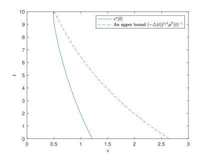
(a) $\gamma=0.5$

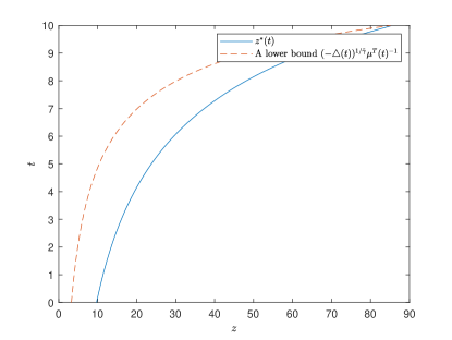
(b) $\gamma=1.5$

Figure 2. Images of $z^{*}(t)$.

The retirement boundaries in dual variables are shown in Figure 3. The retirement boundaries when fixing $w\equiv 1$ (in one variable $y$ only) are also plotted, see Figure 4. Unlike Yang and Koo (2018) and other related literature, no monotonicity results can be expected for the $y-$retirement boundary, even in the constant wage rate model. As we consider a time depend leisure preference here, the agent will enjoy less leisure gains when time involves. As such, early retirement is a better choice, and Figure 4 shows that retirement region gets smaller with time. In the existing literature, such as Yang and Koo (2018) or Dybvig and Liu (2010), they consider time independent leisure preference and show that the retirement boundary increases with time. Our results are consistent with them when setting $K(\cdot)\equiv 1.1$ for $0<\gamma<1$. However, when $\gamma>1$, the retirement boundary always decreases with time under the choice $K(\cdot)\equiv 0.9$.

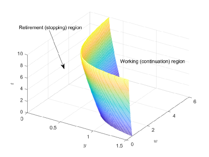
(a) $\gamma=0.5$

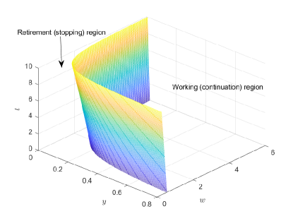
(b) $\gamma=1.5$

Figure 3. Retirement boundary in $(y,w)$-axis.

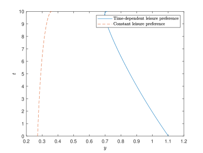
(a) $\gamma=0.5$

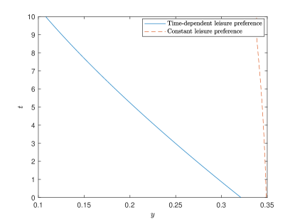
(b) $\gamma=1.5$

Figure 4. Retirement boundary in $y$-axis when $w\equiv 1$.

5. Retirement Boundaries and Optimal Strategies in Terms of Primal Variables

In this section, we show the retirement boundary expressed by primal variables $(x,h,w)$, and provide the optimal investment and consumption strategies. The relation of the primal problem (LABEL:primalproregular) and dual problem (3.16) is revealed in Theorem 3.5. The validity of Theorem 3.5 will be verified first. Based on the primal-dual relation, the retirement boundary w.r.t. $(y,w)$ in Section 4 can be transformed to be expressed w.r.t. $(x,h,w)$. By replication, we show the feedback forms of optimal consumption and investment strategies, which are functions of the de facto wealth $x-p^{T}(t)h$ and wage $w$. Numerical implications of the retirement boundary and optimal strategies are presented. We find the discontinuities of optimal strategies at retirement boundary intuitively.

5.1. The primal-dual relation and characterization of $\mathcal{G}_{t}$

In this section, we present Lemma 5.1 to show that the condition in Theorem 3.5 holds. The optimal stopping time in terms of dual variables can also be obtained by the relation of $z$ with $(y,w)$.

Lemma 5.1.

Let $z^{*}$ be as in Section 4, $y>0$, $w>0$ and $t\in[0,T_{1})$ be fixed. Define

$$\hat{\tau}_{y}=\left\{\begin{array}[]{ll}\inf\{t\leq T_{1}:\ \ (Y^{t,y}(s))^{1/(1-\gamma)}(\mathcal{W}^{t,w}(s))^{\gamma/(1-\gamma)}\leq z^{*}(s)\},&0<\gamma<1,\\ \inf\{t\leq T_{1}:\ \ (Y^{t,y}(s))^{1/(1-\gamma)}(\mathcal{W}^{t,w}(s))^{\gamma/(1-\gamma)}\geq z^{*}(s)\},&\gamma>1.\end{array}\right.$$

Then, $\hat{\tau}_{y}$ is the optimal stopping time of Problem (3.16), and satisfies the condition that $\hat{\tau}_{y+\varepsilon}\to\hat{\tau}_{y}$ almost surely as $\varepsilon\to 0\pm$.

Proof.

See Appendix D. ∎

In fact, in the case of the utility functions specified in Section 4, the allowed region $\mathcal{G}_{t}$ in Remark 5 is equal to its upper bound $\mathcal{E}_{t}$. Thus the results in Theorem 3.5 can be extended to the whole set $\mathcal{G}_{t}$.

Lemma 5.2.

Under the setting of Section 4, we have $\mathcal{G}_{t}=\mathcal{E}_{t}$ and the dual relation (3.18) holds in $\mathcal{G}_{t}$.

Proof.

See Appendix D. ∎

Now we characterize the retirement boundary in the primal variables $(x,h,w)$.

Lemma 5.3.

Define the primal map $\mathscr{P}$ as

$$\mathscr{P}_{t,w}(y)=-W_{y}(t,y,w),$$

and define the primal and dual continuation regions, respectively, as

$$\mathcal{C}^{p}_{t,w}=\{(x,h):\ \ (x,h,w)\in\mathcal{G}_{t},\ \ V>\bar{U}\},$$

$$\mathcal{C}^{d}_{t,w}=\{y>0:\ \ W>\tilde{V}-q(t)yw\}.$$

Then $\mathcal{C}^{p}_{t,w}=\widehat{\mathcal{C}^{p}_{t,w}}\triangleq\{(x,h):\ x-p^{T}(t)h+q(t)w\in\mathscr{P}_{t,w}\mathcal{C}^{d}_{t,w}\}$.

Proof.

See Appendix D. ∎

Remark 8.

It follows from Remark 7 that $\mathscr{P}_{t,w}$ is surjective.

Proposition 5.4.

The retirement boundary can be expressed in primal variables as $\{(t,x,h,w):(x,h)\in\partial\mathcal{C}^{p}_{t,w}\}$, where $\partial\mathcal{C}^{p}_{t,w}=\{(x,h):x-p^{T}(t)h+q(t)w\in\mathscr{P}_{t,w}\partial\mathcal{C}^{d}_{t,w}\}$. In particular, we have

$$\partial\mathcal{C}_{t,w}^{p}=\{(x,h):\ \ x-p^{T}(t)h=G^{*}(t)w\},$$ (5.1)

$$\mathcal{C}_{t,w}^{p}=\{(x,h):\ \ x-p^{T}(t)h<G^{*}(t)w\},$$

where $G^{*}(t)=\tilde{\gamma}H(t)z^{*}(t)^{-\tilde{\gamma}}$, with $H$ defined by the expression $\tilde{V}(t,z)=H(t)z^{-\tilde{\gamma}}$ based on (3.20).

Proof.

See Appendix D. ∎

We see that $x$ and $h$ appear in a whole part as de facto wealth in the retirement boundary. This phenomenon will be found in the feedback forms of optimal strategies. Proposition 5.4 also shows that the retirement boundary is expressed by a linear relationship among $(x,h,w)$.

5.2. Numerical illustrations of primal retirement boundary

Proposition 5.4 establishes the relationship between the retirement boundary in the dual and primal variables, and provides semi-explicit form of it. As such, we can present some numerical results of the retirement boundary.

First, we display the retirement boundary in $(x,h,w)$-axis at time $t=0,5,8$, which are illustrated in Figures 5 and 6. Because $(x,h,w)$ has a linear relationship in Proposition 5.4, the retirement boundaries are all planes for fixed time $t$. Besides, not all $(x,h)$ are in the allowed region. The entire side of the plane with the retirement region is contained in $\mathcal{D}_{t}\times\{w>0\}$, thus in the allowed region. The continuation region is composed of the intersection of the other side of the plane and the allowed region $\mathcal{G}_{t}$. On the plane $w=0$, we know $\mathcal{D}_{t}=\mathcal{G}^{0}_{t}$ (see (2.10), (2.9) and (3.11)), thus the agent does not have initial wealth and will choose to work.

Our figures are the first to describe the retirement boundary with three state variables: wage, habit and wealth. These figures reveal much more economic implications than previous studies. We observe from Figures 5 and 6 that the agent with higher habit level will continue to work to maintain the standard of life. Besides, when the agent has larger wealth or less wage rate, he will choose to retire to enjoy the leisure gains. As time goes by, the agent is expected to receive less future labour income. Thus the importance of wage rate on the agent’s retirement decision decreases. Figure 5 show that the retirement surface evolves closer to the $(h,w)$ plane with time. The critical level of wage rate that pushes one to retire becomes larger. The above results are all consistent for $0<\gamma<1$ and $\gamma>1$.

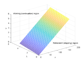
(a) $t=0$

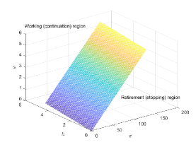
(b) $t=5$

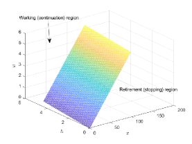
(c) $t=8$

Figure 5. Retirement boundary in $(x,h,w)$-axis, $\gamma=0.5$.

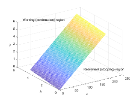
(a) $t=0$

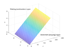
(b) $t=5$

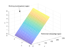
(c) $t=8$

Figure 6. Retirement boundary in $(x,h,w)$-axis, $\gamma=1.5$.

Next, fixing $w=1$, we illustrate the movement of the retirement boundary in $(x,h)$-axis with time, which is displayed in Figure 7. An elder agent will be more likely to retire and Figure 7 shows that the retirement region becomes larger with time.

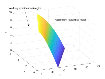
(a) $\gamma=0.5$

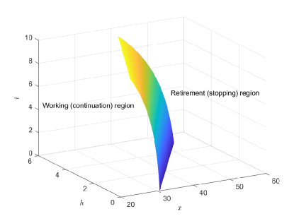
(b) $\gamma=1.5$

Figure 7. Retirement boundary in $(x,h)$-axis, $w=1$.

For clarity, we show the evolution of retirement boundaries with time for $h$ and $x$ by fixing $x=80,w=1$ and $h=6,w=1$, respectively. As we introduce habit formation in our work, we are mostly interested in the effects of habit parameters on the agent’s retirement decision. The retirement boundaries for $(\alpha,\beta)=(0.2,0.4)$ (the benchmark), $(0.1,0.4)$ and $(0.3,0.4)$ are plotted in both cases. The results are reported in Figures 8 and 9. Figure 8 shows that if the weight $\alpha$ of consumption in habit is larger, the agent is more likely to retire even with a smaller standard of life. The importance of habit level on the agent’s retirement decision decreases with time. Therefore, the critical value of $h$ is a decreasing function of time. We can conclude from the figures that, the introduction of habit formation dramatically increases the wealth level that pushes the agent to retire, i.e., he needs to work longer to satisfy his higher standard of life. Moreover, the greater $\alpha$, the more this increase. (2.4) means that with a larger $\alpha$, the past consumption is more important when deciding the current standard of life. As such, the agent has to work longer if he is more addicted to the past level of consumption. This is consistent with the findings of Figure 8, because a larger $\alpha$ leads to lower critical standard of life and later retirement.

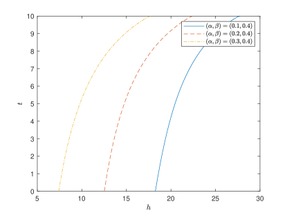
(a) $\gamma=0.5$

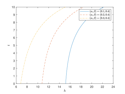
(b) $\gamma=1.5$

Figure 8. Retirement boundary in $(h,t)$-axis, $w=1$, $x=80$.

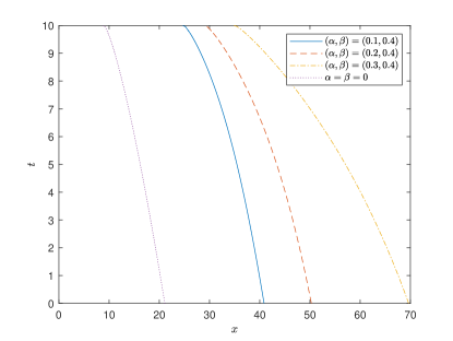
(a) $\gamma=0.5$

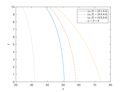
(b) $\gamma=1.5$

Figure 9. Retirement boundary in $(x,t)$-axis, $w=1$, $h=6$.

5.3. Optimal consumption and portfolio

In this subsection, we characterize the optimal consumption and investment strategies. We expect to express them in feed-back forms in $(t,x,h,w)$. Because unlike the last subsection, we mainly focus on the behaviors of optimal strategies in continuation region, $\tilde{V}$ is not enough to derive the optimal strategies. As the financial market is complete, the strategies can be replicated based on the value of $W$. However, $W$ is only known as a semi-explicit form with $z^{*}$.

Theorem 5.5.

The optimal consumption-investment strategies $(c^{*},\pi^{*})$ can be expressed in the following feed-back forms $c^{*}(t)=C^{*}(t,X^{*}(t),h^{*}(t),\mathcal{W}(t))$ and $\pi^{*}(t)=\Pi^{*}(t,X^{*}(t),h^{*}(t),\mathcal{W}(t))$, where $X^{*}$ is solved by SDE (2.3), and $h^{*}$ is solved by ODE (2.4) after substituting $\pi^{*}$ and $c^{*}$ for $\pi$ and $c$. The functions $C^{*}$ and $\Pi^{*}$ which are defined on $\{(t,x,h,w):t\in[0,T_{1}),(x,h,w)\in\mathcal{G}_{t}\}$, can be expressed by:

$$C^{*}(t,x,h,w)=\left\{\begin{array}[]{ll}I_{U_{1}}(y\mu^{T}(t))+h,&{\rm if\ }(x,h)\in\mathcal{C}^{p}_{t,w},\\ I_{U_{2}}(y\mu^{T}(t))+h,&{\rm otherwise},\end{array}\right.$$ (5.4)

$$\Pi^{*}(t,x,h,w)=\left\{\begin{array}[]{ll}\sigma^{-1}(-\sigma_{w}q(t)w-\sigma_{w}wW_{yw}(t,y,w)+\kappa yW_{yy}(t,y,w)),&{\rm if\ }(x,h)\in\mathcal{C}^{p}_{t,w},\\ (\tilde{\gamma}+1)\sigma^{-1}\kappa(x-p^{T}(t)h),&{\rm otherwise},\end{array}\right.$$ (5.7)

where $y=\mathscr{P}_{t,w}^{-1}(x-p^{T}(t)h+w)$.

Proof.

See Appendix D. ∎

Based on Theorem 5.5, we can show the sensitivity analysis of $c^{*}$ and $\pi^{*}$ numerically. $x$, $h$ appear as a whole value of de facto wealth $x-p^{T}(t)h$ (see Remark 3) in the strategies. We are interested in the effects of wage and de facto wealth on the real consumption rate $\mathscr{H}c^{*}=c^{*}-h$. The strategies at time $t=0$ and $t=8$ are plotted, respectively.

The numerical results are in Figures 10 and 11. When $\gamma>1$, the agent has a consumption jump-down at retirement, which is consistent with Chen, Hentschel, and Xu (2018) and Dybvig and Liu (2010). Figure 10 partially explains the retirement consumption puzzle as in Banks, Blundell, and Tanner (1998). However, $\gamma>1$ in Chen, Hentschel, and Xu (2018), Dybvig and Liu (2010) and the marginal utility after retirement decreases. As sated in Hurd and Rohwedder (2003), the agent naturally consumes less due to decrease of the marginal utility. Based on 2001 survey data, Ameriks, Caplin, and Leahy (2007) shows that more than 55% people expect a fall in consumption, while less than 8% people expect an increase after retirement. Thus there is still a minority of people consuming more after retirement. We observe from Figure 11 that agent with risk aversion $0<\gamma<1$ has a consumption jump-up at retirement. In the case $0<\gamma<1$, the marginal utility after retirement increases which implies that consumption after retirement increases. Conversely, we may also deduce that most people have a risk aversion parameter larger than 1, which is documented in Azar (2006) ($\gamma$ is between 4.2 and 5.4) and Schechter (2007) ($\gamma\approx 1.92$).

From Figures 10 and 11, we see that when wage or the de facto wealth increases, the agent has more wealth and will consume more. Besides, the consumption increases slower when the “wealth-habit-wage” triplet approaches the retirement boundary. In other words, when the agent takes retirement into consideration, he will hesitate to consume more, although with more de facto wealth or wage.

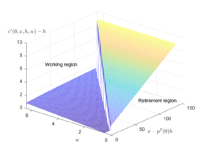
(a) $t=0$

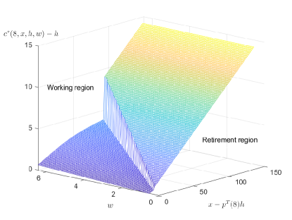
(b) $t=8$

Figure 10. Optimal consumption, $\gamma=0.5$.

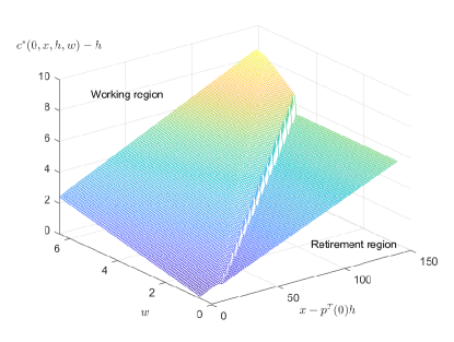
(a) $t=0$

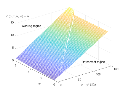
(b) $t=8$

Figure 11. Optimal consumption, $\gamma=1.5$.

Figures 12 and 13 are results about the optimal proportion of risky investment $\pi^{*}(t,x,h,w)/x$ for $\gamma=0.5$ and $\gamma=1.5$, respectively. For simplicity, we only investigate how this proportion changes with de facto wealth when fixing $h=1$. We observe that the surface of optimal investment has drastic variations and there are singularities around the retirement boundary. These singularities arise from the second order derivatives in the expression of $\Pi^{*}$ and the fact that $\hat{w}_{zz}(t,z)$ is not continuous at $z^{*}(t)$ (see Figure 1).

Figures 12 and 13 all suggest a decline of proportion in stock for elder agent, which is observed by the real data in Coile and Milligan (2009)(US) and Spicer, Stavrunova, and Thorp (2016)(Australia). Interestingly, unlike consumption, the optimal investment strategies always have a jump down at retirement boundary, no matter $\gamma=0.5$ or $\gamma=1.5$. This means that people will always withdraw their investment in risky asset upon retirement to hedge the risk of unemployment, which is the so-called “saving for retirement”. The patterns of the investment behavior are different for $\gamma=0.5$ and $\gamma=1.5$. In the continuation region, the evolution of optimal investment near the retirement boundary is drastic for $\gamma=1.5$ while smooth for $\gamma=0.5$. When $\gamma>1$ and the agent approaches the retirement boundary, he will suddenly, yet strategically, raise his risk investment and adjust his consumption simultaneously to prepare for incoming retirement. However, when $\gamma<1$, the agent behaves more conservatively in consumption while more aggressive in investment before retirement: he consumes generally less than the case $\gamma>1$, and adjusts the investment gradually.

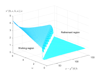
(a) $t=0$

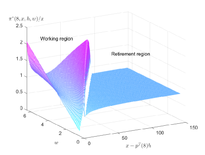
(b) $t=8$

Figure 12. Optimal portfolio proportion, $\gamma=0.5$.

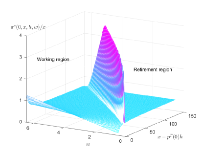
(a) $t=0$

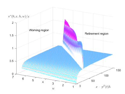
(b) $t=8$

Figure 13. Optimal portfolio proportion, $\gamma=1.5$.

6. Conclusions

This paper investigates a retirement decision and optimal consumption-investment model with addictive habit formation. Different from existing literature, three state variables, namely the wealth $x$, the habit $h$ and the wage rate $w$, affect the agent’s decision in this paper. We model this optimization problem as a StopCP in finite time horizon. The mixture of control and stopping in this model requires the establishment of dual relation, which becomes more difficult in the presence of habit formation. Using utility transformation, modified habit reduction method and dual method, we obtain an equivalent dual pure optimal stopping problem in finite time horizon. The rather complicated dual relation is then established by investigating the continuity of optimal stopping time with respect to state variables.

After specifying the preferences, we present and prove the verification theorem that connects the dual value function with parabolic free boundary problems. Using this, we provide the retirement boundaries in the dual and primal variables, feedback forms of optimal investment and consumption strategies. The numerical results have clear economic interpretations. We show that the enough amount of de facto wealth, when exceeding an critical proportion of wage, will trigger the retirement. We also find that, people who are more addicted to past consumption have a larger working region, and will choose to work longer to maintain the standard of life. “Retirement consumption puzzle” and “saving for retirement” can also be explained to some extent in our framework.

In this paper, we consider the addictive linear habit formation and a concave utility function for simplicity. Consideration of drawdown/ratcheting constraints as in Angoshtari, Bayraktar, and Young (2019) may be interesting. Besides, we can further study non-addictive habit formation, such as reference to past maximum of consumption in Deng, Li, Pham, and Yu (2020). More general extensions of the StopCP-based on retirement modeling to the non-concave utility with habit to characterize loss aversion as in van Bilsen, Laeven, and Nijman (2020) and van Bilsen and Laeven (2020) are left for future studies. We expect the arguments developed in the first three sections to be useful when investigating these problems.

Acknowledgements. The authors acknowledge the support from the National Natural Science Foundation of China (Grant No.11901574, No.11871036, and No.11471183). The authors are grateful to Lin He and Yang Liu for their comments and suggestions. The authors also thank the members of the group of Insurance Economics and Mathematical Finance at the Department of Mathematical Sciences, Tsinghua University for their feedbacks and useful conversations.

Appendix A Proofs of Lemmas 3.8 and 3.4

Proof of Lemma 3.8.

The proof is similar with various literature with habit formation by modifying the terminal fixed time to a stopping time, see Proposition 2.3.3 in Yu (2012) for example. However, as some details of calculations change, we provide the proof for completeness. We first see from (2.7) that for $s\leq u\leq T_{1}$:

$$h(u)=h(s)m(u)/m(s)+\alpha m(u)\int_{s}^{u}\hat{c}(v)/m(v)\mathrm{d}v.$$ (A.1)

A combination of $c=\hat{c}+h$ and Fubini’s theorem shows for any fixed $\tau\in\mathbb{S}_{t}^{T_{1}}$,

$$\int_{s}^{\tau}c(u)\xi^{t}(u)\mathrm{d}u = \int_{s}^{\tau}\hat{c}(u)\xi^{t}(u)\mathrm{d}u+\int_{s}^{\tau}h(u)\xi^{t}(u)\mathrm{d}u$$

$$= \int_{s}^{\tau}\hat{c}(u)\xi^{t}(u)\mathrm{d}u+\int_{s}^{\tau}h(s)m(u)/m(s)\xi^{t}(u)\mathrm{d}u$$

$$\ \ \ \ +\alpha\int_{s}^{T_{1}}\int_{s}^{u}\frac{m(u)}{m(v)}\xi^{t}(u)\hat{c}(v)I_{\{u\leq\tau\}}\mathrm{d}v\mathrm{d}u$$

$$= \int_{s}^{\tau}\hat{c}(u)\xi^{t}(u)\mathrm{d}u+\int_{s}^{\tau}h(s)m(u)/m(s)\xi^{t}(u)\mathrm{d}u$$

$$\ \ \ \ +\alpha\int_{s}^{T_{1}}\hat{c}(u)\left(\int_{u}^{T_{1}}\frac{m(v)}{m(u)}\xi^{t}(v)I_{\{v\leq\tau\}}\mathrm{d}v\right)\mathrm{d}u$$

$$= \int_{s}^{\tau}\hat{c}(u)\left(\xi^{t}(u)+\alpha\int_{u}^{\tau}\frac{m(v)}{m(u)}\xi^{t}(v)\mathrm{d}v\right)\mathrm{d}u$$

$$\ \ \ \ +h(s)\xi^{t}(s)\int_{s}^{\tau}\frac{m(u)}{m(s)}\frac{\xi^{t}(u)}{\xi^{t}(s)}\mathrm{d}u.$$

Taking $\mathbb{E}_{s}$ on both sides of the last equation derives the desired result. ∎

Proof of Lemma 3.4.

Let $M(s)=\mathbb{E}_{s}[\xi^{t}(\tau)p^{T}(\tau)m(\tau)]$. Obviously, $\{M(s\wedge\tau):t\leq s\leq T_{1}\}$ is a square-integrable and uniformly integrable continuous martingale. Based on definitions in Lemma 3.8, we have that for $s\in[t,\tau]$

$$\left\{\begin{array}[]{lll}p^{\tau}(s)&=\mathbb{E}_{s}\left[\int_{s}^{T}\frac{m(u)}{m(s)}\frac{\xi^{t}(u)}{\xi^{t}(s)}\mathrm{d}u\right]-\mathbb{E}_{s}\left[\int_{\tau}^{T}\frac{m(u)}{m(s)}\frac{\xi^{t}(u)}{\xi^{t}(s)}\mathrm{d}u\right]\\ &=p^{T}(s)-\mathbb{E}_{s}\mathbb{E}_{\tau}\left[\int_{\tau}^{T}\frac{m(u)}{m(\tau)}\frac{\xi^{t}(u)}{\xi^{t}(\tau)}\mathrm{d}u\right]m(\tau)\xi^{t}(\tau)(m(s)\xi^{t}(s))^{-1}\\ &=p^{T}(s)-(\xi^{t}(s)m(s))^{-1}M(s),\\ \mu^{\tau}(s)&=\mu^{T}(s)-\alpha(\xi^{t}(s)m(s))^{-1}M(s).\end{array}\right.$$ (A.6)

As such,

$$\mathbb{E}_{s}\left[\int_{s}^{\tau}\!\hat{c}(u)\xi^{t}(u)\mu^{T}(u)\mathrm{d}u\right]\!-\!\mathbb{E}_{s}\left[\int_{s}^{\tau}\hat{c}(u)\xi^{t}(u)\mu^{\tau}(u)\mathrm{d}u\right]\!=\!\alpha\mathbb{E}_{s}\left[\int_{s}^{\tau}\hat{c}(u)m(u)^{-1}M(u)\mathrm{d}u\right].$$ (A.7)

On the other hand, we see from (A.1) that

$$\mathrm{d}(h(u)/m(u))=\alpha\hat{c}(u)/m(u)\mathrm{d}u.$$

Define $\tau_{n}=\inf\{t\leq t^{\prime}\leq T:\int_{t}^{t^{\prime}}|m(u)^{-1}h(u)|^{2}\mathrm{d}<M>_{u}\geq n\}\vee s$. Applying Itô’s formula to $h(u)M(u)m(u)^{-1}$, we obtain

$$h(\tau\wedge\tau_{n})M(\tau\wedge\tau_{n})m(\tau\wedge\tau_{n})-h(s)m(s)^{-1}M(t) = \alpha\int_{s}^{\tau\wedge\tau_{n}}M(u)m(u)^{-1}\hat{c}(u)\mathrm{d}u$$ (A.8)

$$\!\!+\int_{s}^{\tau\wedge\tau_{n}}m(u)^{-1}h(u)\mathrm{d}M(u).$$

Taking $\mathbb{E}_{s}$ on both sides of (A.8),

$$\mathbb{E}_{s}h(\tau\wedge\tau_{n})M(\tau\wedge\tau_{n})m(\tau\wedge\tau_{n})-h(s)m(s)^{-1}M(s)=\alpha\mathbb{E}_{s}\int_{s}^{\tau\wedge\tau_{n}}M(u)m(u)^{-1}\hat{c}(u)\mathrm{d}u.$$

Letting $n\to\infty$ and using monotonous convergence theorem and dominated convergence theorem, we have

$$\mathbb{E}_{s}h(\tau)M(\tau)m(\tau)-h(s)m(s)^{-1}M(s)=\alpha\mathbb{E}_{s}\int_{s}^{\tau}M(u)m(u)^{-1}\hat{c}(u)\mathrm{d}u.$$ (A.9)

Combining (A.7) and (A.9) gives

$$\mathbb{E}_{s}h(\tau)p^{T}(\tau)\xi^{t}(\tau)-h(s)m(s)^{-1}M(s)=\mathbb{E}_{s}\left[\int_{s}^{\tau}\hat{c}(u)\xi^{t}(u)\mu^{T}(u)\mathrm{d}u\right]-\mathbb{E}_{s}\left[\int_{s}^{\tau}\hat{c}(u)\xi^{t}(u)\mu^{\tau}(u)\mathrm{d}u\right].$$

Thus, plugging (A.6) to replace the term $h(s)m(s)^{-1}M(s)$ in the last equation completes the proof. ∎

Appendix B Proof of Theorem 3.5

To verify the dual relation, we quote some classical arguments in the proof of main results in Karatzas and Wang (2000). Because our financial model with habit formation is different from Karatzas and Wang (2000), the procedure to prove the theorem is similar while much more complex. Recall that we have already proved the inequality (3.17), i.e., we have the one side inequality of (3.18):

$$V(t,x,h,w)\leq\inf_{y>0}\{W(t,y,w)+y(x-p^{T}(t)h)+yq(t)w\}.$$

Then we want to verify the converse inequality of (3.18). It is sufficient to show that (3.18) holds for some particular $y$. First, we present the following lemmas:

Lemma B.1.

We have the following asymptotic results for function $\tilde{U}$:

$$\lim_{y\to 0}\inf_{0\leq t\leq T_{1}}I_{\tilde{U}}(t,y)=\infty,$$ (B.1)

$$\lim_{y\to\infty}\sup_{0\leq t\leq T_{1}}I_{\tilde{U}}(t,y)=0,$$ (B.2)

$$\sup_{0\leq t\leq T_{1}}I_{\tilde{U}}(t,y)\leq C(1+y^{-K}),$$ (B.3)

where $C$ and $K>0$ are constants.

Proof.

By similar arguments in the proof of Lemma B.4 (using convexity of $\tilde{V}$), we conclude that

$$I_{\tilde{U}}(t,y)=-\partial_{y}\tilde{V}(t,y)=\mathbb{E}\left[\int_{t}^{T}\xi^{t}(u)I_{U_{2}}(u,yY^{t,1}(u))\mathrm{d}u\right].$$

(B.3) follows from bounded assumption of $I_{U_{2}}$ and (B.2) follows from the asymptotic properties of $I_{U_{2}}$ and monotone convergence theorem. In fact, (B.1) can be obtained by the same arguments, as we have the following estimation:

$$I_{\tilde{U}}(t,y) \geq\mathbb{E}\left[\int_{T}^{T_{1}}\xi^{t}(u)I_{U_{2}}(u,yY^{t,1}(u))\mathrm{d}u\right]$$

$$\geq\mathbb{E}\left[\left(\int_{T}^{T_{1}}\xi(u)I_{U_{2}}(u,e^{2\rho T}\xi(u)/\inf_{0\leq t\leq T_{1}}\xi(u))\mathrm{d}u\right)/\sup_{0\leq t\leq T_{1}}\xi(t)\right].\qed$$

Lemma B.2.

For $\tau\in\mathbb{S}_{t}^{T_{1}}$ and fixed $t\in[0,T_{1}]$, define

$$\mathcal{X}_{t,\tau}(y)=\mathbb{E}\left[\int_{t}^{\tau}\xi^{t}(u)\mu^{T}(u)I_{U_{1}}(Y^{t,y}(u)\mu^{T}(u))+I_{\tilde{U}}(t,Y^{t,y}(\tau))\xi^{t}(\tau)\right].$$

Then, $\forall\mathbf{x}>0$, there exists $y>0$ such that

$$\mathcal{X}_{t,\hat{\tau}_{y}}(y)=\mathbf{x}.$$

Furthermore, $W$ is differentiable in $y$ in $(0,\infty)$ and

$$W_{y}(t,y,w)=-\mathcal{X}_{t,\hat{\tau}_{y}}(y)-w\mathbb{E}e^{-\rho(\hat{\tau}_{y}-t)}Y^{t,1}(\hat{\tau}_{y})\mathcal{W}^{t,1}(\hat{\tau}_{y})q(\hat{\tau}_{y}).$$ (B.4)

Proof.

To prove (B.4), first we have

$$\lim_{y\to 0}\mathcal{X}_{t,\hat{\tau}_{y}}(y)=\infty,\quad\lim_{y\to\infty}\mathcal{X}_{t,\hat{\tau}_{y}}(y)=0,$$

which can be easily verified by Lemma B.1. We claim that $\mathcal{X}_{\hat{\tau}_{y}}(y)$ is continuous in $y$. In fact, the estimation

$$|\mathcal{X}_{t,\hat{\tau}_{y}}(y)|\leq C(2T_{1}M+1)(\sup_{t\leq s\leq T_{1}}\xi^{t}(s))(1+\delta^{-K}\sup_{t\leq s\leq T_{1}}(Y^{t,1}(s))^{-K})$$

holds uniformly for $y\in[\delta,\infty)$, where $M=\sup_{t\in[0,T]}\mu^{T}(t)$. The right side of the inequality is integrable by Burkholder-Davies-Gundy’s inequality. As such, using dominated convergence theorem, we conclude that $\mathcal{X}_{t,\hat{\tau}_{y}}(y)$ is continuous in $y$ on $[\delta,\infty)$. As $\delta>0$ is arbitrary , $\mathcal{X}_{t,\hat{\tau}_{y}}(y)$ is continuous in $(0,\infty)$. Therefore, the mapping $(0,\infty)\to(0,\infty):\ y\mapsto\mathcal{X}_{\hat{\tau}_{y}}(y)$ is surjective. To prove (B.4), we begin with some estimation of the difference of $W$ based on convexity. For $\eta\in\mathbb{R}$ near 0, we have

$$W(t,y+\eta,w) -W(t,y,w)$$

$$\leq \mathbb{E}\left[\int_{t}^{\hat{\tau}_{y+\eta}}e^{-\rho(u-t)}[\hat{V}_{1}((y+\eta)\mu^{T}(u)Y^{t,1}(u))-\hat{V}_{1}(y\mu^{T}(u)Y^{t,1}(u))]\mathrm{d}u\right]$$

$$+\mathbb{E}e^{-\rho(\hat{\tau}_{y+\eta}-t)}(\tilde{V}(t,(y+\eta)Y^{t,1}(\hat{\tau}_{y+\eta}))-\tilde{V}(t,yY^{t,1}(\hat{\tau}_{y+\eta})))$$

$$-\eta w\mathbb{E}e^{-\rho(\hat{\tau}_{y+\eta}-t)}Y^{t,1}(\hat{\tau}_{y+\eta})\mathcal{W}^{t,1}(\hat{\tau}_{y+\eta})q(\hat{\tau}_{y+\eta})$$

$$\leq \mathbb{E}\left[\int_{t}^{\hat{\tau}_{y+\eta}}\eta e^{-\rho(u-t)}\mu^{T}(u)Y^{t,1}(u)\hat{V}_{1}^{\prime}(\mu^{T}(u)Y^{t,y+\eta}(u))\mathrm{d}u\right]$$

$$+\mathbb{E}he^{-\rho(\hat{\tau}_{y+\eta}-t)}Y^{t,1}(\hat{\tau}_{y+\eta})\tilde{V}^{\prime}_{y}(t,Y^{t,y+\eta}(\hat{\tau}_{y+\eta}))$$

$$-\eta w\mathbb{E}e^{-\rho(\hat{\tau}_{y+h}-t)}Y^{t,1}(\hat{\tau}_{y+h})\mathcal{W}^{t,1}(\hat{\tau}_{y+h})q(\hat{\tau}_{y+h})$$

$$= -\eta\mathbb{E}\left[\int_{t}^{\hat{\tau}_{y+\eta}}\xi^{t}(u)I_{\hat{V}_{1}}(\mu^{T}(u)Y^{t,y+\eta}(u))\mathrm{d}u+\xi^{t}(\hat{\tau}_{y+\eta})I_{\tilde{U}}(t,Y^{t,y+\eta}(\hat{\tau}_{y+\eta}))\right]$$

$$+\eta w\mathbb{E}e^{-\rho(\hat{\tau}_{y+\eta}-t)}Y^{t,1}(\hat{\tau}_{y+\eta})\mathcal{W}^{t,1}(\hat{\tau}_{y+\eta})$$

$$= -\eta\mathcal{X}_{t,\hat{\tau}_{y+\eta}}(y+\eta)-\eta w\mathbb{E}e^{-\rho(\hat{\tau}_{y+\eta}-t)}Y^{t,1}(\hat{\tau}_{y+\eta})\mathcal{W}^{t,1}(\hat{\tau}_{y+\eta})q(\hat{\tau}_{y+\eta}).$$

Dividing by $\eta$ on both sides of the last inequalities and letting $\eta\to 0+$, we have

$$W_{y+}(t,y,w)\leq-\mathcal{X}_{\hat{\tau}_{y}}(y)-w\mathbb{E}e^{-\rho(\hat{\tau}_{y}-t)}Y^{t,1}(\hat{\tau}_{y})\mathcal{W}^{t,1}(\hat{\tau}_{y})q(\hat{\tau}_{y}).$$

Conversely, letting $\eta\to 0-$, we get

$$W_{y-}(t,y,w)\geq-\mathcal{X}_{\hat{\tau}_{y}}(y)-w\mathbb{E}e^{-\rho(\hat{\tau}_{y}-t)}Y^{t,1}(\hat{\tau}_{y})\mathcal{W}^{t,1}(\hat{\tau}_{y})q(\hat{\tau}_{y}).$$

Combining the last two inequalities, (B.4) holds. ∎

Proof of Theorem 3.5.

First, $\mathbb{E}\{b(\hat{\tau}_{y})\xi^{t}(\hat{\tau}_{y})\}$ is continuous in $y$, which can be proved similarly as the continuity of $\mathcal{X}_{\hat{\tau}_{y}}(y)$. As $\mathcal{X}_{t,\hat{\tau}_{y}}(y)$ maps $(0,\infty)$ onto $(0,\infty)$, $\mathcal{X}_{\hat{\tau}_{y}}(y)+\mathbb{E}b(\hat{\tau}_{y})\xi^{t}(\hat{\tau}_{y}))$ maps $(0,\infty)$ onto $(q(t)w,\infty)$. Now, we choose $y^{*}>0$ such that

$$\mathcal{X}_{t,\hat{\tau}_{y^{*}}}(y^{*})+\mathbb{E}b(\hat{\tau}_{y^{*}})\xi^{t}(\hat{\tau}_{y^{*}})=x-p^{T}(t)h+q(t)w.$$

Based on Lemma 3.4, the last equation is

$$\mathbb{E}\left[\int_{t}^{\hat{\tau}_{y^{*}}}\xi^{t}(u)\mu^{\hat{\tau}_{y^{*}}}(u)\hat{c}^{*}(u)\mathrm{d}u+B^{*}\xi^{t}(\hat{\tau}_{y^{*}})\right]+hp^{\hat{\tau}_{y^{*}}}(t)=x+b(t),$$

with $\hat{c}^{*}(u)=I_{U_{1}}(u,Y^{t,y^{*}}(u)\mu^{T}(u))$ and $B^{*}=I_{\tilde{U}}(\hat{\tau}_{y^{*}},Y^{t,y^{*}}(\hat{\tau}_{y^{*}}))+h(\hat{\tau}_{y^{*}})p^{T}(\hat{\tau}_{y^{*}})+b(\hat{\tau}_{y^{*}})$. This implies that $(\hat{c}^{*},\hat{\tau}_{y^{*}})\in\hat{\mathcal{B}}_{=}$ and all inequalities in (3.4) are in fact equalities. Thus, the proof is completed. ∎

Appendix C Proofs of the results in Section 4

In this section we prove the properties of $\hat{w}$ satisfying (4.6) and verify Theorem 4.2. All properties will be satisfied by $\tilde{w}$. Let $F=\hat{w}-\tilde{V}+q$. We need the following results.

Lemma C.1.

Let $F_{\alpha}(t,z)=F(t,\alpha(t)z)$, then

$$(\partial_{t}+\mathscr{L}_{\alpha})F_{\alpha}\big{|}_{(t,z)}=(\partial_{t}+\mathscr{L}_{Z})F\big{|}_{(t,\alpha(t)z)},$$

where

$$\mathscr{L}_{\alpha}=\frac{\sigma_{z}^{2}}{2}z^{2}\partial_{zz}+(\mu_{z}-\alpha^{\prime}(t)/\alpha(t))z\partial_{z}+\vartheta.$$

Proof.

This lemma is easily verified by directly calculating the derivatives of $F_{\alpha}$ as follows:

$$\partial_{t}F_{\alpha}=\partial_{t}F+\alpha^{\prime}(t)z\partial_{z}F\big{|}_{(t,\alpha(t)z)},$$

$$\partial_{z}F_{\alpha}=\alpha(t)\partial_{z}F\big{|}_{(t,\alpha(t)z)},$$

$$\partial_{zz}F_{\alpha}=\alpha(t)^{2}\partial_{zz}F\big{|}_{(t,\alpha(t)z)}.$$

The left sides of the last three equations are all calculated at point $(t,z)$. ∎

We now turn to showing the monotonicity of $F$, which is the basis of the analysis of $z^{*}$.

Lemma C.2.

1. If $0<\gamma<1$, $F$ increases with respect to $z$.

2. If $\gamma>1$, $F$ decreases with respect to $z$.

Proof.

We first prove the case $\gamma>1$. $\forall\delta^{\prime}>1$, consider $F_{\delta^{\prime}}(t,z)=F(t,\delta^{\prime}z)$ . Based on Lemma C.1 and (4.8), we conclude that $F_{\delta^{\prime}}$ satisfies

$$\left\{\begin{aligned} &(-\partial_{t}-\mathscr{L}_{Z})F_{\delta^{\prime}}=\triangle(t)(\mu^{T}(t)\delta^{\prime}z)^{-\tilde{\gamma}}+1,{\rm\ if\ }\ F_{\delta^{\prime}}(t,z)>0,\\ &(-\partial_{t}-\mathscr{L}_{Z})F_{\delta^{\prime}}\geq\triangle(t)(\mu^{T}(t)\delta^{\prime}z)^{-\tilde{\gamma}}+1,{\rm\ if\ }\ F_{\delta^{\prime}}(t,z)=0,\\ &F_{\delta^{\prime}}(T_{1},\cdot)=0.\end{aligned}\right.$$

It follows that

$$\triangle(t)(\mu^{T}(t)\delta^{\prime}z)^{-\tilde{\gamma}}<\triangle(t)(\mu^{T}(t)z)^{-\tilde{\gamma}}.$$

As such, if the comparison principles of variational inequalities (cf. Lemma A.6 in Yan, Liang, and Yang (2015)) can be applied, we can get the desired conclusion. Note that in order to apply Lemma A.6 in Yan, Liang, and Yang (2015), we only need to verify that $\tilde{w}$ and $\tilde{V}$ are of polynomial growth. This is true because

$$(-\partial_{t}-\mathscr{L}_{Z})F\leq-\frac{\delta}{2}z^{-\tilde{\gamma}}+1,{\rm\ in\ }\mathcal{C}.$$

Hence, we choose

$$F_{0}(t,z)=-1/\vartheta-Az^{-\tilde{\gamma}}+B^{\prime}z^{\lambda_{+}}$$

such that

$$(-\partial_{t}-\mathscr{L}_{Z})F_{0}=-\frac{\delta}{2}z^{-\tilde{\gamma}}+1,{\rm\ in\ }\mathcal{C},$$

where the constants $A$ and $\lambda_{+}$ are explained in the proof of Theorem 4.5 (see Figure 14 for the relation of $F_{0}$, $\hat{F}$ and $F$). $B^{\prime}$ is a constant which is large enough. Thus, we have $F_{0}\geq\hat{F}\geq 0$, and in particular, $F_{0}(T_{1},\cdot)\geq 0$, $F_{0}\geq 0=F$ on $\partial\mathcal{C}$. Then we apply strong maximum principle for elliptic equations to conclude that $F$ has growth rate no more than $z^{-\tilde{\gamma}+\lambda_{+}}$, hence has polynomial growth. The fact that $-\tilde{\gamma}>0$ when $\gamma>1$ is crucial in this case. Note that the above argument also guarantees the boundness of $F$ when $z\to 0+$. As such, the comparison on $\{z=0\}$ is always valid. The monotonicity when $\gamma>1$ has been proved. To prove the case $0<\gamma<1$, define $\tilde{F}(t,z)=F(t,1/z)$, we have

$$\left\{\begin{aligned} &(-\partial_{t}-\mathscr{L}_{\rm inv})\tilde{F}=\triangle(t)(\mu^{T}(t))^{-\tilde{\gamma}}z^{\tilde{\gamma}}+1,{\rm\ if\ }\ \tilde{F}(t,z)>0,\\ &(-\partial_{t}-\mathscr{L}_{\rm inv})\tilde{F}\geq\triangle(t)(\mu^{T}(t))^{-\tilde{\gamma}}z^{\tilde{\gamma}}+1,{\rm\ if\ }\ \tilde{F}(t,z)=0,\\ &\tilde{F}(T_{1},\cdot)=0,\end{aligned}\right.$$

where

$$\mathscr{L}_{\rm inv}=\frac{\sigma_{z}^{2}}{2}z^{2}\partial_{zz}+(\sigma_{z}^{2}-\mu_{z})z\partial_{z}+\vartheta.$$

Noting that in this case $\tilde{F}$ has polynomial growth, comparison principles are valid. As such, repeating the argument for the case $\gamma>1$, we conclude that $F(t,1/z)$ is decreasing in $z$, and $F$ is increasing in $z$. ∎

Now we present the characterization of the stopping boundary in Problem (4.3).

Proposition C.3.

If $0<\gamma<1$, $\mathcal{C}=\{(t,z):0\leq t<T_{1},z>z^{*}(t)\}$. If $\gamma>1$, $\mathcal{C}=\{(t,z):0\leq t<T_{1},0<z<z^{*}(t)\}$. Here, $z^{*}(\cdot)$ is a $[0,\infty]$-valued function, and is Lipschitz continuous on $\{t:z^{*}(t)<\infty\}$.

Proof.

We only prove the case $\gamma>1$ as the proof when $0<\gamma<1$ is similar. Based on Lemma C.2, we know that $F$ is decreasing in $z$. For any $t\in[0,T_{1})$, let $z^{*}(t)\triangleq\inf\{z>0:F=0\}$. Then it is easy to verify that $\mathcal{C}=\{(t,z):0<z<z^{*}(t)\}$. ∎

Proof of Theorem 4.5.

All things have been proved except the boundness of $z^{*}$ (above and below). We first prove the case $\gamma>1$. Assume that $\mu_{z}<0$ and $-\mu_{z}$ is large enough (to be determined later). Based on Proposition 4.4 and Assumption 3, we know that if $z<M^{1/\tilde{\gamma}}/\mu^{T}(0)$, then $\forall t\in[0,T_{1})$, $z<M^{\tilde{\gamma}/1}/\mu^{T}(t)\leq(-\triangle(t))^{\tilde{\gamma}/1}/\mu^{T}(t)$. Thus $\triangle(t)>-(\mu^{T}(t)z)^{\tilde{\gamma}}$ and $(t,z)\in\mathcal{C}$. This gives a lower bound: $z^{*}(t)\geq M^{1/\tilde{\gamma}}/\mu^{T}(0)>0$. For the upper bound, we consider the following auxiliary function:

$$\hat{F}(t,z)=\left\{\begin{array}[]{ll}0,&z\geq z_{\infty},\\ -1/\vartheta-Az^{-\tilde{\gamma}}+Bz^{\lambda_{+}},&0<z<z_{\infty}.\end{array}\right.$$ (C.1)

The constants $A$, $B$, $z_{\infty}$ in (C.1) will be explained successively. Here, we consider the quadratic function:

$$Q(\lambda)=\frac{\sigma_{z}^{2}}{2}\lambda^{2}+(\mu_{z}-\frac{\sigma_{z}^{2}}{2})\lambda+\vartheta.$$

Now in (C.1), $\lambda_{+}$ is the positive root of $Q(\lambda)=0$. It is easy to check that $\lambda_{+}>1$ (as $\mu_{z}<0$). Moreover, we set the constants as

$$A=-\delta/2Q(-\tilde{\gamma}),$$

$$z_{\infty}=\left(\frac{\lambda_{+}}{-\vartheta A(\lambda_{+}+\tilde{\gamma})}\right)^{-1/\tilde{\gamma}},$$

$$B=\frac{-\tilde{\gamma}A}{\lambda_{+}}z_{\infty}^{-\tilde{\gamma}-\lambda_{+}}.$$

By the fact $0<-\tilde{\gamma}<1<\lambda_{+}$, obviously, $Q(-\tilde{\gamma})<0$ and $A$, $B$, $z_{\infty}>0$. We see that $\hat{F}$ is independent of $t$ and is in $C^{1}(\mathbb{R}_{+})\cap C^{2}(\mathbb{R}_{+}\backslash z_{\infty})$. Moreover, $\frac{\partial{\hat{F}}}{\partial z}<0$ for $z\in(0,z_{\infty})$. As such, it follows that $\hat{F}$ is decreasing on $(0,z_{\infty})$ with $\hat{F}(z_{\infty})=0$, and satisfies

$$(-\partial-\mathscr{L}_{Z})\hat{F}=-\frac{\delta}{2}z^{-\tilde{\gamma}}+1,{\rm\ if\ }0<z<z_{\infty}.$$

Besides, $\forall z>z_{\infty}$, we have

$$-\frac{\delta}{2}z^{-\tilde{\gamma}}+1 <-\frac{\delta}{2}z_{\infty}^{-\tilde{\gamma}}+1$$

$$=-\frac{\delta}{2}\frac{\lambda_{+}}{-\vartheta A(\lambda_{+}+\tilde{\gamma})}+1$$

$$=1-Q(-\tilde{\gamma})\frac{\lambda_{+}}{\vartheta(\lambda_{+}+\tilde{\gamma})}.$$

Direct calculations show that the right side of the last equation is not greater than $0$ if and only if

$$\lambda_{+}\tilde{\gamma}+\frac{2}{\sigma_{z}^{2}}\vartheta\leq\vartheta.$$

Noting that

$$\lambda_{+}=\frac{\frac{\sigma_{z}^{2}}{2}-\mu_{z}+\sqrt{(\frac{\sigma_{z}^{2}}{2}-\mu_{z})^{2}-2\sigma_{z}^{2}\vartheta}{}}{\sigma_{z}^{2}},$$

we have $\lambda_{+}\to+\infty$ if $\mu_{z}\to-\infty$. Choosing $\mu_{z}$ small enough, we can prove that

$$\lambda_{+}\tilde{\gamma}+\frac{2}{\sigma_{z}^{2}}\vartheta\leq\vartheta.$$

In this case we conclude that $\hat{F}$ satisfies

$$\left\{\begin{aligned} &(-\partial_{t}-\mathscr{L}_{Z})\hat{F}=-\frac{\delta}{2}z^{-\tilde{\gamma}}+1,{\rm\ if\ }\ \hat{F}(t,z)>0,\\ &(-\partial_{t}-\mathscr{L}_{Z})\hat{F}\geq-\frac{\delta}{2}z^{-\tilde{\gamma}}+1,{\rm\ if\ }\ \hat{F}(t,z)=0,\\ &\hat{F}(T_{1},\cdot)\geq 0.\end{aligned}\right.$$

Applying the comparison principles, we obtain that $F\leq\hat{F}$. In particular, $\{(t,z):0\leq t<T_{1},z>z_{\infty}\}\subset\mathcal{S}$. This implies that $z^{*}(t)\leq z_{\infty},\forall t\in[0,T_{1})$, which is what we need.

Next we reduce the condition that $\mu_{z}<0$ is small enough. Choosing $\alpha(t)=e^{Kt}$ with $K>0$ large enough in Lemma C.1, we find that $F_{\alpha}(t,z)=F(t,e^{Kt}z)$ satisfies the variational inequalities with first order term $\mu_{z}-K$ in the differential operator. Then, by the arguments above, we know that $e^{-Kt}z^{*}(t)$ is bounded above, thus so is $z^{*}$. Finally, an application of transformation $z\mapsto 1/z$ just like the proof of Proposition C.2 completes the proof in the case $0<\gamma<1$. ∎

Figure 14. The images of $F(t,\cdot)$ for some fixed $t\in[0,T_{1})$. Dashed line: $\hat{F}$. Dotted line: $F_{0}$.

Remark 9.

It is easily seen from the proof that $(-\triangle(t))^{1/\tilde{\gamma}}\mu^{T}(t)^{-1}$ serves as a(n) lower/upper bound for $t\in[0,T_{1})$ when $\gamma>1$ and $0<\gamma<1$, respectively.

Finally, we will need some properties of $\hat{w}$ that are useful in the proof of Theorem 4.2.

Lemma C.4.

$z\mapsto\hat{w}(t,z)$ is convex on $(0,\infty)$.

Proof.

First, we consider $\gamma>1$. For fixed $\lambda\in[0,1]$, denote $G^{1}_{\lambda}(t,\mathbf{z})=\hat{w}(t,\lambda z_{1}+(1-\lambda)z_{2})$, $G^{2}_{\lambda}(t,\mathbf{z})=\lambda\hat{w}(t,z_{1})+(1-\lambda)\hat{w}(t,z_{2})$, $H^{1}_{\lambda}(t,\mathbf{z})=\tilde{V}(t,\lambda z_{1}+(1-\lambda)z_{2})-q(t)$ and $H^{2}_{\lambda}(t,\mathbf{z})=\lambda\tilde{V}(t,z_{1})+(1-\lambda)\tilde{V}(t,z_{2})-q(t)$, where $\mathbf{z}^{T}=(z_{1},z_{2})\in\mathbb{R}_{+}^{2}$. Define

$$\mathbf{L}=\frac{\sigma_{z}^{2}}{2}\mathbf{z}^{T}\partial_{\mathbf{z}\mathbf{z}}\mathbf{z}+\mu_{z}\mathbf{z}^{T}\partial_{\mathbf{z}}+\vartheta,$$

where $\partial_{\mathbf{z}\mathbf{z}}$ and $\partial_{\mathbf{z}}$ are interpreted as Hessian and gradient operators. We can easily check

$$\left\{\begin{aligned} &(-\partial_{t}-\mathbf{L}_{Z})G^{1}_{\lambda}=(\lambda z_{1}+(1-\lambda)z_{2})^{-\tilde{\gamma}}\mu^{T}(t)^{-\tilde{\gamma}}/\tilde{\gamma},{\rm\ if\ }G^{1}_{\lambda}(t,\mathbf{z})>H^{1}_{\lambda}(t,\mathbf{z}),\\ &(-\partial_{t}-\mathbf{L}_{Z})G^{1}_{\lambda}\geq(\lambda z_{1}+(1-\lambda)z_{2})^{-\tilde{\gamma}}\mu^{T}(t)^{-\tilde{\gamma}}/\tilde{\gamma},{\rm\ if\ }G^{1}_{\lambda}(t,\mathbf{z})=H^{1}_{\lambda}(t,\mathbf{z}),\\ &G^{1}_{\lambda}(T_{1},\cdot)=H^{1}_{\lambda}(T_{1},\cdot),\end{aligned}\right.$$

and

$$\left\{\begin{aligned} &(-\partial_{t}-\mathbf{L}_{Z})G^{2}_{\lambda}=(\lambda z_{1}^{-\tilde{\gamma}}+(1-\lambda)z_{2}^{-\tilde{\gamma}})\mu^{T}(t)^{-\tilde{\gamma}}/\tilde{\gamma},{\rm\ if\ }G^{2}_{\lambda}(t,\mathbf{z})>H^{2}_{\lambda}(t,\mathbf{z}),\\ &(-\partial_{t}-\mathbf{L}_{Z})G^{2}_{\lambda}\geq(\lambda z_{1}^{-\tilde{\gamma}}+(1-\lambda)z_{2}^{-\tilde{\gamma}})\mu^{T}(t)^{-\tilde{\gamma}}/\tilde{\gamma},{\rm\ if\ }G^{2}_{\lambda}(t,\mathbf{z})=H^{2}_{\lambda}(t,\mathbf{z}),\\ &G^{2}_{\lambda}(T_{1},\cdot)=H^{2}_{\lambda}(T_{1},\cdot).\end{aligned}\right.$$

Note that comparison principles are also valid for higher dimensional variational inequalities. Thus convexity of $\tilde{w}$ follows from convexity of $z\mapsto z^{-\tilde{\gamma}}/\tilde{\gamma}$ as $0<-\tilde{\gamma}<1$.

In the case $0<\gamma<1$, we consider $\bar{w}(t,z)=\hat{w}(1,1/z)$. Then growth estimation for $\gamma>1$ derives $|\bar{F}|\leq C(1+z^{K})$, i.e., $|\hat{w}|\leq C(1+z^{-K})$. Based on Theorem 4.5, when $z$ is small enough, $\hat{w}=\tilde{V}-q$ is convex. Then we restrict our domain to $z_{1}\geq z_{1}^{0}$ and $z_{2}\geq z_{2}^{0}$ such that $G^{1}_{\lambda}\leq G^{2}_{\lambda}$ holds true on the part of parabolic boundary $[0,T_{1})\times\{z_{1}^{0}\}\times[z_{2}^{0},\infty)\cup[0,T_{1})\times[z_{1}^{0},\infty)\times\{z_{2}^{0}\}$. Because $G^{1}_{\lambda}$ and $G^{2}_{\lambda}$ are of polynomial growth on the restricted domain, comparison principles are also valid. Thus, we complete the proof because $z\mapsto z^{-\tilde{\gamma}}/\tilde{\gamma}$ is still convex. ∎

Lemma C.5.

$\hat{w}$ satisfies (4.5).

Proof.

We only need to prove Lemma C.5 when $\gamma>1$. Using the bounds of $F$ and $\tilde{V}$, we have $|\hat{w}|\leq C(1+z^{K})$. Based on the fact that $\tilde{V}$ is decreasing in $z$ (which can be checked directly, noticing $\hat{V}_{2}<0$), and $F=\hat{w}-\tilde{V}+q$ is decreasing in $z$, we know that $\hat{w}$ is decreasing in $z$. Noting the convexity of $\hat{w}$, we have that $\partial_{z}\hat{w}(t,\cdot)\leq 0$ is increasing in $z$. Furthermore, for $0<z<z_{0}$, we have

$$\hat{w}(t,z)-\hat{w}(t,z_{0})\geq\partial_{z}\hat{w}(t,z_{0})(z-z_{0}),$$

which implies $\partial_{z}\hat{w}(t,z_{0})\geq-Cz_{0}^{-1}$ because $\hat{w}$ is bounded when $z\to 0$. Therefore when $z\to 0$, $\partial_{z}\hat{w}\geq-C(1+z^{-K})$. Thus, $|\partial_{z}\hat{w}|\leq C(1+z^{-K})$. ∎

Based on Lemmas C.4 and C.5, we now give the proof of Theorem 4.2.

Proof of Theorem 4.2.

Step1: $\tilde{w}\leq\hat{w}$. Fix any $(t,z)\in\mathcal{N}_{T_{1}}$ and $\tau\in\mathbb{S}_{t}^{T_{1}}$. We know from the proofs above that $\partial\mathcal{C}\cap\mathcal{N}_{T_{1}}$ can be expressed as a curve $\{(t,z):0\leq t\leq T_{1},z=z^{*}(t)\}$, where $z^{*}$ is Lipschitz continuous, and bounded above and below from $0$ on $[0,T_{1}]$. As such, the local time formula holds (see Section II.3.5 in Peskir and Shiryaev (2006)). The conditions (3.5.10)-(3.5.13) in Peskir and Shiryaev (2006) should be satisfied, i.e., the convexity of $\hat{w}$ in Lemma C.4 is needed. We conclude that, $\tilde{\mathbb{P}}^{t,z}$-almost surely,

$$e^{\vartheta\tau}\hat{w}(\tau,Z(\tau))-e^{\vartheta t}\hat{w}(t,z) =\int_{t}^{\tau}e^{\vartheta u}(\partial_{t}+\mathscr{L}_{Z})\hat{w}(u,Z(u))I_{\{Z(u)\neq z^{*}(u)\}}\mathrm{d}u$$

$$\ \ \ \ +\int_{t}^{\tau}\sigma_{z}e^{\vartheta u}Z(u)\partial_{z}\hat{w}(u,Z(u))I_{\{Z(u)\neq z^{*}(u)\}}\mathrm{d}\tilde{B}(u)$$

$$\leq-\int_{t}^{\tau}e^{\vartheta u}\hat{V}_{1}(u,Z(u))\mathrm{d}u$$

$$\ \ \ \ +\int_{t}^{\tau}\sigma_{z}e^{\vartheta u}Z(u)\partial_{z}\hat{w}(u,Z(u))I_{\{Z(u)\neq z^{*}(u)\}}\mathrm{d}\tilde{B}(u).$$

The indicator in the first term of right side can be estimated by property (4.4). Then taking expectation $\tilde{\mathbb{E}}^{t,z}$ on both sides of the last inequality, we conclude from the growth condition of $\partial_{z}\hat{w}$ that the expectation of the Itô’s integral is zero. Noting the fact $\hat{w}\geq\tilde{V}-q$, we have

$$\tilde{\mathbb{E}}^{t,z}\left[e^{\vartheta\tau}(\tilde{V}(\tau,Z(\tau))-q(\tau))+\int_{t}^{\tau}e^{\vartheta u}\hat{V}_{1}(u,Z(u))\mathrm{d}u\right]\leq e^{\vartheta t}\hat{w}(t,z),$$

which yields $\tilde{w}\leq\hat{w}$.

Step2: $\tilde{w}\geq\hat{w}$. Let $(t,z)\in\mathcal{C}$ and define $\tau^{*}=\inf\{s\geq t:(u,Z(u))\notin\mathcal{C}\}$. Now let $\tau=\tau_{\varepsilon}\triangleq(\tau^{*}-\varepsilon)\wedge t$ in the calculation of Step 1. Then we get

$$\tilde{\mathbb{E}}^{t,z}e^{\vartheta\tau_{\varepsilon}}\hat{w}(\tau_{\varepsilon},Z(\tau_{\varepsilon}))=e^{\vartheta t}\hat{w}(t,z)-\mathbb{E}\left[\int_{t}^{\tau_{\varepsilon}}e^{\vartheta u}\hat{V}_{1}(u,Z(u))\mathrm{d}u\right],$$

as $(u,Z(u))\in\mathcal{C}$ on $[t,\tau_{\varepsilon}]$. Letting $\varepsilon\rightarrow 0$ on both sides of the last equation, because of the growth conditions of $\hat{w}$ and $\hat{V}_{1}$, we have

$$\tilde{\mathbb{E}}^{t,z}\left[e^{\vartheta\tau^{*}}(\tilde{V}(\tau,Z(\tau^{*}))-q(\tau^{*}))+\int_{t}^{\tau^{*}}e^{\vartheta u}\hat{V}_{1}(u,Z(u))\mathrm{d}u\right]=e^{\vartheta t}\hat{w}(t,z),$$

which implies $\tilde{w}\geq\hat{w}$ in $\mathcal{C}$. Moreover, in $\mathcal{N}_{T_{1}}\backslash\mathcal{C}$ we have $\hat{w}=\tilde{V}-q\leq\tilde{w}$. The proof is thus completed. ∎

Proof of Theorem 4.6.

Applying Itô’s formula involving local time to $e^{\vartheta T_{1}}F(T_{1},Z(T_{1}))-e^{\vartheta t}F(t,z)$ and setting $z=z^{*}(t)$, we obtain (4.9) and (4.10), which is valid as $F$ is the linear combination of two convex functions. The fact that $F=0$ when $z=z^{*}(t)$ is also used.

Next we prove the terminal condition in Theorem 4.6. Again we only need to prove it when $\gamma>1$. By transformation $z\mapsto 1/z$, the result remains true when $0<\gamma<1$.

The boundness and Lipschitz continuous properties guarantee the existence of limit $z^{*}(T_{1}-)=\lim_{t\to T_{1}}z^{*}(t)$. Proposition 4.4 derives $z^{*}(T_{1}-)\geq\alpha(T_{1})$ with the definition $\alpha(t)\triangleq(-\triangle(t))^{1/\tilde{\gamma}}\mu^{T}(T_{1})^{-1}$.

If $z^{*}(T_{1}-)>\alpha(T_{1})$, we find an interval $\alpha(T_{1})<z_{1}<z_{2}<z^{*}(T_{1}-)$ and sufficiently small $\varepsilon>0$ such that $[T_{1}-\varepsilon,T_{1})\times[z_{1},z_{2}]\subset\mathcal{C}$. Define $F_{K}(t,z)=F(t,e^{Kt}z)$. Based on Lemma C.1, we know that $F_{K}$ satisfies

$$\left\{\begin{aligned} &(-\partial_{t}-\mathscr{L}_{K})F_{K}=-(\alpha(t)^{-1}e^{Kt}z)^{-\tilde{\gamma}}+1,{\rm\ if\ }F_{K}(t,z)>0,\\ &(-\partial_{t}-\mathscr{L}_{K})F_{K}\geq-(\alpha(t)^{-1}e^{Kt}z)^{-\tilde{\gamma}}+1,{\rm\ if\ }F_{K}(t,z)=0,\\ &F_{K}(T_{1},\cdot)=0.\end{aligned}\right.$$

Now choose $K>0$ large enough such that $-(\alpha(t)^{-1}e^{Kt}z)^{-\tilde{\gamma}}$ decreases with $t$, which is possible because $|\triangle(t)^{\prime}|$ and $|\mu^{T}(t)^{\prime}|$ are both bounded from above. Then, $\forall t\in[t_{0},T_{1})$, comparing $F_{K}(t-t_{0},z)$ and $F_{K}(t,z)$ on $[t_{0},T_{1})\times\mathbb{R}_{+}$, and noting the fact $F_{K}(T_{1}-t_{0},z)\geq 0=F_{K}(T_{1},z)$, we conclude that $F_{K}$ decreases with $t$. As such, $\partial_{t}F_{K}\leq 0$ in $\mathcal{N}_{T_{1}}$. If we let $\varepsilon<\frac{1}{K}\log(z_{2}/z_{1})$, then for any $z\in I\triangleq(z_{1}e^{-K(T_{1}-\varepsilon)},z_{2}e^{-KT_{1}})$, we have $z_{1}e^{-Kt}<z<z_{2}e^{-Kt}$, $\forall t\in[T_{1}-\varepsilon,T_{1}]$. As such, $(t,e^{Kt}z)\in\mathcal{C}$, $(F_{K}(t,z)>0$ and

$$-\partial_{t}F_{K}(t,z)-\mathscr{L}_{K}F_{K}(t,z)=-(\alpha(t)^{-1}e^{Kt}z)^{-\tilde{\gamma}}+1.$$

Letting $t\to T_{1}$ on both sides of the last equation, as $z>\alpha(T_{1})e^{-KT_{1}}$, we have

$$\limsup_{t\to T_{1}}(-(\alpha(t)^{-1}e^{Kt}z)^{-\tilde{\gamma}}+1)\leq-(\alpha(T_{1})^{-1}e^{KT_{1}}z)^{-\tilde{\gamma}}+1<0.$$

As $F_{K}(T_{1},z)=0$, if we can prove $\mathscr{L}_{K}F_{K}(t,z)\to 0$ for a.s. $z$ on $I$, as $t\to T_{1}-$, then $\partial_{t}F_{K}(T_{1}-,z)>0$ a.s. on $I$, which is a contradiction. In fact, $\forall z_{3}>z_{4}>0$,

$$F_{K}(t,z_{3})-F_{K}(t,z_{4})=\int_{z_{3}}^{z_{4}}\partial_{z}F_{K}(t,z^{\prime})\mathrm{d}z^{\prime}.$$

Dominated convergence theorem shows

$$0=\int_{z_{3}}^{z_{4}}\partial_{z}F_{K}(T_{1}-,z^{\prime})\mathrm{d}z^{\prime}.$$

However, $F_{K}$ is decreasing in $z$. Thus we have $F_{K}(T_{1}-,z^{\prime})=0$ on $[z_{3},z_{4}]$. Moreover

$$\partial_{z}F_{K}(t,z_{3})-\partial_{z}F_{K}(t,z_{4})=\int_{z_{3}}^{z_{4}}\partial_{zz}F_{K}(t,z^{\prime})\mathrm{d}z^{\prime}.$$

Applying Fatou’s lemma, we have

$$\int_{z_{3}}^{z_{4}}\partial_{zz}F_{K}(T_{1}-,z^{\prime})\mathrm{d}z^{\prime}\leq 0.$$

Then convexity of $F_{K}(t,\cdot)$ implies $\partial_{zz}F_{K}(T_{1}-,z^{\prime})\geq 0$, which in turn implies $\partial_{zz}F_{K}(T_{1}-,z^{\prime})=0$, a.s. on $[z_{3},z_{4}]$. Thus, by arbitrariness of $z_{3}$ and $z_{4}$, it is also true a.s. on $I$. As such, $\mathscr{L}_{K}F_{K}\to 0$, which is a contradiction. Therefore, the assumption that $z^{*}(T_{1}-)>\alpha(T_{1})$ is not true, thus, we have $z^{*}(T_{1}-)=\alpha(T_{1})$. ∎

Appendix D Proof of results in Section 5

Proof of Lemma 5.1.

We only prove Lemma 5.1 when $0<\gamma<1$, because the proof of the case $\gamma>1$ is similar. Denote $z_{y}=y^{1/(1-\gamma)}w^{\gamma/(1-\gamma)}$. We first note that

$${\rm Law}(\hat{\tau}_{y}|\mathbb{P})={\rm Law}(\tilde{\tau}_{y}|\tilde{\mathbb{P}})$$ (D.1)

with $\tilde{\tau}_{y}=\inf\{t\leq s\leq T_{1}:Z^{t,z_{y}}(s)\leq z^{*}(s)\}$. Based on optimal stopping theory (cf. Chapter I, Theorem 2.4 in Peskir and Shiryaev (2006)), $\tilde{\tau}_{y}$ is optimal for Problem (4.3). Based on Lemma 4.1, $\hat{\tau}_{y}$ is also optimal for Problem (3.16). Then we need to prove the continuity. By (D.1), it is sufficient to prove the continuity of $\tilde{\tau}_{y}$ in the sense of $\tilde{\mathbb{P}}$-almost surely.

If $z_{y}<z^{*}(t)$, then for sufficiently small $\varepsilon$, $\tilde{\tau}_{y+\varepsilon}\equiv t$. As such, we only need to consider $z_{y}\geq z^{*}(t)$. We prove it in the following two steps:

Step 1: Show that $\tilde{\tau}_{y+\varepsilon}\to\tilde{\tau}_{y}$, as $\varepsilon\searrow 0$, for $z_{y}\geq z^{*}(t)$.

Step 2: Show that $\tilde{\tau}_{y^{\prime}}\to\tilde{\tau}_{y}$, as $y^{\prime}\nearrow y$, for $z_{y}>z^{*}(t)$.

Proof of Step 1: We rewrite $\tilde{\tau}_{y}$ as $\tilde{\tau}_{y}=\inf\{t\leq s\leq T_{1}:Z^{t,1}(s)\leq z^{*}(s)/z_{y}\}$ and similarly for $\tilde{\tau}_{y+\varepsilon}$ (see Figure 15-(a) for graphical illustration). Using the fact that $z_{y}$ increases with $y$, we have $\tilde{\tau}_{y+\varepsilon}\searrow\tilde{\tau}^{\prime}\geq\tilde{\tau}_{y}$. Define $B_{k}=\{\omega:\ \tilde{\tau}^{\prime}-\tilde{\tau}_{y}>1/k\}$ and $B=\bigcup_{k=1}^{\infty}B_{k}$, we aim to prove $\tilde{\mathbb{P}}(B)=0$. It is sufficient to prove $\tilde{\mathbb{P}}(B_{k})=0$. Define $A_{k}^{\varepsilon}\triangleq\{\omega:\ \tilde{\tau}_{y+\varepsilon}-\tilde{\tau}_{y}\geq 1/k\}$ for any $k$. Noting the following observations: under the conditional law of $\tilde{\mathbb{P}}(\cdot|\tilde{\tau}_{y}=t^{\prime})$,

$$\tilde{\tau}_{y+\varepsilon}-\tilde{\tau}_{y} =\tilde{\tau}_{y+\varepsilon}-t^{\prime}$$

$$=\inf\{t^{\prime}\leq s\leq T_{1}:Z^{t^{\prime},z^{*}(t^{\prime})/z_{y}}(s)\leq z^{*}(s)/z_{y+\varepsilon}\}-t^{\prime}$$

$$=\inf\{0\leq s\leq T-t^{\prime}:Z^{t^{\prime},z^{*}(t^{\prime})z_{y+\varepsilon}/z_{y}}(s+t^{\prime})\leq z^{*}(s+t^{\prime})\},$$

we have (see Figure 15-(b))

$${\rm Law}(\tilde{\tau}_{y+\varepsilon}-\tilde{\tau}_{y}|\tilde{\mathbb{P}}(\cdot|\tilde{\tau}_{y}=t^{\prime}))={\rm Law}(\tilde{\tau}^{*}|\tilde{\mathbb{P}}^{t^{\prime},z^{*}(t^{\prime})z_{y+\varepsilon}/z_{y}}),$$

where

$$\tilde{\tau}^{*}=\inf\{0\leq s\leq T_{1}-t^{\prime}:Z(s+t^{\prime})\leq z^{*}(s+t^{\prime})\}.$$

The regularities of the boundary $\{z=z^{*}(s)\}$ and the process $(\cdot+t^{\prime},Z(\cdot+t^{\prime}))$ derive

$$\lim_{\varepsilon\searrow 0}\tilde{\mathbb{P}}^{t^{\prime},z^{*}(t^{\prime})z_{y+\varepsilon}/z_{y}}(\tilde{\tau}^{*}\geq 1/k)=0,$$

which in turn implies

$$\lim_{\varepsilon\searrow 0}\tilde{\mathbb{P}}(A_{k}^{\varepsilon}|\tilde{\tau}_{y}=t^{\prime})=0.$$

Then dominated convergence theorem gives

$$\lim_{\varepsilon\searrow 0}\tilde{\mathbb{P}}(A_{k}^{\varepsilon}) =\lim_{\varepsilon\searrow 0}\int_{t}^{T_{1}}\tilde{\mathbb{P}}(A_{k}|\tilde{\tau}_{y}=t^{\prime})\tilde{\mathbb{P}}(\tilde{\tau}_{y}\in\mathrm{d}t)$$

$$=0.$$

As such,

$$\tilde{\mathbb{P}}(\lim_{\varepsilon\searrow 0}\tilde{\tau}_{y+\varepsilon}-\tilde{\tau}_{y}\geq 1/k) =\lim_{\varepsilon\searrow 0}\tilde{\mathbb{P}}(\tilde{\tau}_{y+\varepsilon}-\tilde{\tau}_{y}\geq 1/k)$$

$$=\lim_{\varepsilon\searrow 0}\tilde{\mathbb{P}}(A_{k}^{\varepsilon})$$

$$=0.$$

Thus the proof of Step 1 is completed.

Figure 15. Continuity of $\tilde{\tau}_{y}$.

Proof of Step 2: Using monotonicity of $z_{y^{\prime}}$ in $y^{\prime}$, we know $\tilde{\tau}_{y^{\prime}}\nearrow\tilde{\tau}_{2}\leq\tilde{\tau}_{y}$. Based on regularity of process $Z$, we have

$$z_{y^{\prime}}Z^{t,1}(\tilde{\tau}_{y^{\prime}})\leq z^{*}(\tilde{\tau}_{y^{\prime}}).$$

Letting $y^{\prime}\to y$,

$$z_{y}Z^{t,1}(\tilde{\tau}_{2})\leq z^{*}(\tilde{\tau}_{2}),$$

which in turn shows $\tilde{\tau}_{2}\geq\tilde{\tau}_{y}$. Thus, $\tilde{\tau}_{2}=\tilde{\tau}_{y}$. ∎

Proof of Lemma 5.2.

Based on Remark 5, we need to prove $\lim_{y\to\infty}\mathbb{E}[b(\hat{\tau}_{y})\xi^{t}(\hat{\tau}_{y})]=0$. Again we only prove it when $0<\gamma<1$. To this end, we claim that $\hat{\tau}_{y}\to T_{1}$ as $y\to\infty$. The claim is then equivalent to $\tilde{\tau}_{z}\to T_{1}$ when $z\to\infty$ with the notation $\tilde{\tau}_{z}=\inf\{t\leq s\leq T_{1}:Z^{t,z}(s)\leq z^{*}(s)\}$. We expand $z^{*}$ to $z^{**}$ as follows

$$z^{**}(s)=\left\{\begin{array}[]{ll}z^{*}(s),&s\in[0,T_{1}),\\ z^{*}(T_{1}-),&s\in[T_{1},\infty).\end{array}\right.$$

Define $\tilde{\tau}^{\prime}_{z}=\inf\{s\geq t:Z^{t,z}(s)\leq z^{**}(s)\}$. Then it is sufficient to prove $\tilde{\tau}^{\prime}_{z}\to\infty$ as $z\to\infty$. As $\tilde{\tau}^{\prime}_{z}$ increases with $z$, we only need to prove for any fixed $K>0$, $\lim_{z\to\infty}\tilde{\mathbb{P}}(\tilde{\tau}^{\prime}_{z}\leq K)=0$ (using the same argument as in the proof of Lemma 5.1).

Denote $z^{\infty}=\sup\limits_{s\geq 0}z^{**}(s)>0$. We have that $\tilde{\tau}^{\prime}_{z}\geq t+\tilde{\tau}^{\prime\prime}_{z}\triangleq\{s\geq 0:\sigma_{z}\tilde{W}(s)+(\mu_{z}-\frac{\sigma_{z}^{2}}{2})s\leq\log(z^{\infty}/z)\}$. Using measure change, we conclude that for some equivalent measure $\hat{\mathbb{P}}$, and standard Brownian Motion $\hat{W}$ under $\hat{\mathbb{P}}$, $\tilde{\tau}^{\prime\prime}_{z}$ is the first hitting time of $\hat{W}$ to $\log(z^{\infty}/z)/\sigma_{z}$. Thus, we may estimate

$$\hat{\mathbb{P}}(\tilde{\tau}^{\prime}_{z}\leq K)\leq\hat{\mathbb{P}}(\tilde{\tau}^{\prime\prime}_{z}\leq K-t)=\frac{2}{\sqrt{2\pi}}\int_{\log(z^{\infty}/z)/(-\sqrt{K-t}|\sigma_{z}|)}^{\infty}e^{-x^{2}/2}\mathrm{d}x\to 0,$$

as $z\to\infty$. The validity of (3.18) on $\mathcal{G}_{t}$ follows naturally from the proof of Theorem 3.5 as $-W_{y}$ maps $\mathbb{R}_{+}$ onto $\mathbb{R}_{+}$. The proof is completed. ∎

Proof of Lemma 5.3.

Based on Theorem 3.5 and convexity of $W$, we have

$$V(t,x,h,w)=(x-p^{T}(t)h+q(t)w)y+W(t,y,w),y=\mathscr{P}^{-1}_{t,w}(x-p^{T}(t)h+q(t)w).$$

If $y\in\mathcal{C}^{d}_{t,w}$, then (see Lemma 3.19):

$$(x-p^{T}(t)h+q(t)w)y^{*}+W(t,y^{*},w) >(x-p^{T}(t)h+q(t)w)y^{*}+\tilde{V}(t,y^{*})-q(t)y^{*}w$$

$$=y^{*}(x-p^{T}(t)h)+\tilde{V}(t,y^{*}).$$

$$\geq\tilde{U}(t,x-p^{T}(t)h)=\bar{U}(t,x,h),$$

which shows $(x,h)\in\mathcal{C}^{p}_{t,w}$. As such, if $(x,h)\in\widehat{\mathcal{C}^{p}_{t,w}}$, it is clear that $\mathscr{P}^{-1}_{t,w}(x-p^{T}(t)h+q(t)w)\in\mathcal{C}^{d}_{t,w}$. Thus, $(x,h)\in\mathcal{C}^{p}_{t,w}$ and $\widehat{\mathcal{C}^{p}_{t,w}}\subset\mathcal{C}^{p}_{t,w}$.

On the other hand, if $(x,h)\in\mathcal{C}^{p}_{t,w}$, then for $y^{*}=\mathscr{P}^{-1}_{t,w}(x-p^{T}(t)h+q(t)w)$, based on the last part of proof in Lemma B.4, we know that the optimal stopping time $\hat{\tau}_{y^{*}}$ for $W$ is also optimal for $V$. As such, $\hat{\tau}_{y^{*}}>t$, which implies $y^{*}\in\mathcal{C}^{d}_{t,w}$. Therefore $x-p^{T}(t)h+q(t)w=\mathscr{P}_{t,w}y^{*}\in\mathscr{P}_{t,w}\mathcal{C}_{d}$ and the proof is completed. ∎

Proof of Proposition 5.4.

Based on Lemma B.4 and the proof of Lemma 5.2, we know that $\mathscr{P}_{t,w}\mathbb{R}_{+}=(0,\infty)$. As such, if $(x,h,w)\in\mathcal{G}_{t}$, then $x-p^{T}(t)h+q(t)w\notin\mathscr{P}_{t,w}\mathcal{C}^{d}_{t,w}$ if and only if $x-p^{T}(t)h+q(t)w\in\mathscr{P}_{t,w}(\mathbb{R}_{+}\backslash\mathcal{C}^{d}_{t,w})$. ∎

Proof of Theorem 5.5.

The expressions of $c^{*}$ and $\pi^{*}$ outside $\mathcal{C}^{p}_{t,w}$ can be easily obtained by classical methods. The readers are referred to, for example, (6.24) and (6.25) in Englezos and Karatzas (2009). We only need to prove the expressions for $(x,h)\in\mathcal{C}^{p}_{t,w}$. Let $\hat{\tau}_{t,y,w}$ be as in Lemma 5.1. Based on the proof of Theorem 3.5, defining $\hat{c}^{*}(u)=I_{U_{1}}(u,Y^{t,y}(u)\mu^{T}(u))$ and $B^{*}=I_{\tilde{U}}(\hat{\tau}_{t,y.w},Y^{t,y}(\hat{\tau}_{t,y,w}))+h(\hat{\tau}_{t,y,w})p^{T}(\hat{\tau}_{t,y,w})+b(\hat{\tau}_{t,y,w})$, we know that $(\hat{\tau}_{t,y,w},\hat{c}^{*})\in\hat{\mathcal{B}}_{=}$ and all inequalities in (3.4) become equalities. As such, $\tilde{\mathscr{H}}^{-1}(\hat{\tau}_{t,y,w},\hat{c}^{*})\in\mathcal{B}_{=}$ attains maxima in Problem (LABEL:primalproregular). Thus, the expression (5.4) is verified.

Now we prove (5.7). Let $s\geq t$, for $(s,y^{\prime},w^{\prime})$ such that $y^{\prime}\in\mathcal{C}^{d}_{s,w^{\prime}}$, conditioned on $\{s<\hat{\tau}_{t,y,w},Y^{t,y}(s)=y^{\prime},\mathcal{W}^{t,w}(s)=w^{\prime}\}$, $\hat{\tau}_{t,y,w}=\hat{\tau}_{s,y^{\prime},w^{\prime}}$ holds in the sense of distribution under $\mathbb{P}$. Moreover, using Markovian property of $Y$, we have

$$\mathbb{E}\left[e^{-\rho(\hat{\tau}_{t,y,w}-t)}Y^{t,y}(\hat{\tau}_{t,y,w})I_{\tilde{U}}(\hat{\tau}_{t,y,w},Y^{t,y}(\hat{\tau}_{t,y,w}))+e^{-\rho(\hat{\tau}_{t,y,w}-t)}Y^{t,y}(\hat{\tau}_{t,y,w})q(\hat{\tau}_{t,y,w})\mathcal{W}^{t,w}(\hat{\tau}_{t,y,w})\right.$$

$$\ \ \ \ \left.+\int_{s}^{\hat{\tau}_{t,y,w}}e^{-\rho(\hat{\tau}_{t,y,w}-t)}Y^{t,y}(u)\mu^{T}(u)I_{U_{1}}(u,Y^{t,y}(u)\mu^{T}(u))\mathrm{d}u\big{|}Y^{t,y}(s)=y^{\prime},\mathcal{W}^{t,w}(s)=w^{\prime}\right]$$

$$=\mathbb{E}\left[e^{-\rho(\hat{\tau}_{s,y^{\prime},w^{\prime}}-t)}Y^{s,y^{\prime}}(\hat{\tau}_{s,y^{\prime},w^{\prime}})I_{\tilde{U}}(\hat{\tau}_{s,y^{\prime},w^{\prime}},Y^{s,y^{\prime}}(\hat{\tau}_{s,y^{\prime},w^{\prime}}))\right.$$

$$\ \ \ \ +\left[e^{-\rho(\hat{\tau}_{s,y^{\prime},w^{\prime}}-t)}Y^{s,y^{\prime}}(\hat{\tau}_{s,y^{\prime},w^{\prime}})q(\hat{\tau}_{s,y^{\prime},w^{\prime}})\mathcal{W}^{s,w^{\prime}}(\hat{\tau}_{s,y^{\prime},w^{\prime}})\right.$$

$$\ \ \ \ \left.+\int_{s}^{\hat{\tau}_{s,y^{\prime},w^{\prime}}}e^{-\rho(\hat{\tau}_{s,y^{\prime},w^{\prime}}-t)}Y^{s,y^{\prime}}(u)\mu^{T}(u)I_{U_{1}}(u,Y^{s,y^{\prime}}(u)\mu^{T}(u))\mathrm{d}u\right]$$

$$=-W_{y}(s,y^{\prime},w^{\prime})y^{\prime}.$$

Integrating with respect to the distribution of $Y^{t,y}(s)$ and $\mathcal{W}^{t,w}(s)$, for $s\in[t,\hat{\tau}_{t,y,w})$, we have

$$\mathbb{E}_{s}\left[e^{-\rho(\hat{\tau}_{t,y,w}-t)}Y^{t,y}(\hat{\tau}_{t,y,w})I_{\tilde{U}}(\hat{\tau}_{t,y,w},Y^{t,y}(\hat{\tau}_{t,y,w}))+e^{-\rho(\hat{\tau}_{t,y,w}-t)}Y^{t,y}(\hat{\tau}_{t,y,w})q(\hat{\tau}_{t,y,w})\mathcal{W}^{t,w}(\hat{\tau}_{t,y,w})\right.$$

$$\ \ \ \ \left.+\int_{s}^{\hat{\tau}_{t,y,w}}e^{-\rho(\hat{\tau}_{t,y,w}-t)}Y^{t,y}(u)\mu^{T}(u)I_{U_{1}}(u,Y^{t,y}(u)\mu^{T}(u))\mathrm{d}u\right]$$

$$\ \ \ \ =-W_{y}(s,Y^{t,y}(s),\mathcal{W}^{t,w}(s))Y^{t,y}(s).$$

Combining the last equation with (3.6), (3.7) and (3.10), we have

$$\xi^{t}(s)(X(s)+q(s)\mathcal{W}^{t,w}(s))=-W_{y}(s,Y^{t,y}(s),\mathcal{W}^{t,w}(s))e^{\rho(s-t)}\xi^{t}(s)+\xi^{t}(s)p^{T}(s)h(s).$$

Then dividing both sides of the last equations by $\xi^{t}$, taking differential and applying Itô’s formula, we obtain the stochastic differential equation of $\xi^{t}(s)(X(s)+q(s)\mathcal{W}^{t,w})$. Comparing the coefficients of diffusion terms in this SDE with that obtained from (2.3), we have

$$\pi^{*}(s)=\sigma^{-1} (-\sigma_{w}q(s)\mathcal{W}^{t,w}(s)-\sigma_{w}W_{yw}(s,Y^{t,y}(s),\mathcal{W}^{t,w}(s))\mathcal{W}^{t,w}(s)e^{\rho(s-t)}$$

$$+\kappa W_{yy}(s,Y^{t,y}(s),\mathcal{W}^{t,w}(s))Y^{t,y}(s)e^{\rho(s-t)}),$$

which shows that the feed-back form of $\pi^{*}$ in $(y,w)$ is

$$\Pi^{*}(t,y,w)=\sigma^{-1}(-\sigma_{w}q(t)w-\sigma_{w}wW_{yw}(t,y,w)+\kappa yW_{yy}(t,y,w)).$$

At last, applying dual-primal relation $x-p^{T}(t)h+q(t)w=\mathscr{P}_{t,w}y$ proves (5.7). ∎

References

- Abel (1990) Andrew B. Abel. Asset prices under habit formation and catching up with the joneses. The American Economic Review, 80(2):38–42, 1990.
- Ameriks et al. (2007) John Ameriks, Andrew Caplin, and John Leahy. Retirement consumption: Insights from a survey. Review of Economics and Statistics, 89(2):265–274, 2007.
- Angoshtari et al. (2019) Bahman Angoshtari, Erhan Bayraktar, and Virginia R. Young. Optimal dividend distribution under drawdown and ratcheting constraints on dividend rates. SIAM Journal on Financial Mathematics, 10(2):547–577, 2019.
- Azar (2006) Samih Antoine Azar. Measuring relative risk aversion. Applied Financial Economics Letters, 2(5):341–345, 2006.
- Banks et al. (1998) J Banks, R Blundell, and S Tanner. Is there a retirement-savings puzzle? American Economic Review, 88(4):769–788, 1998.
- Campbell and Cochrane (1999) John Y Campbell and John H Cochrane. By force of habit: A consumption-based explanation of aggregate stock market behavior. Journal of Political Economy, 107(2):205–251, 1999.
- Chen et al. (2018) An Chen, Felix Hentschel, and Xian Xu. Optimal retirement time under habit persistence: what makes individuals retire early? Scandinavian Actuarial Journal, 2018(3):225–249, 2018.
- Choi and Koo (2005) Kyoung Jin Choi and Hyeng Keun Koo. A preference change and discretionary stopping in a consumption and porfolio selection problem. Mathematical Methods of Operations Research, 61(3):419–435, 2005.
- Choi et al. (2008) Kyoung Jin Choi, Gyoocheol Shim, and Yong Hyun Shin. Optimal portfolio, consumption-leisure and retirement choice problem with CES utility. Mathematical Finance, 18(3):445–472, 2008.
- Coile and Milligan (2009) Courtney Coile and Kevin Milligan. How household portfolios evolve after retirement: the effect of aging and health shocks. Review of Income and Wealth, 55(2):226–248, 2009.
- Constantinides (1990) George M Constantinides. Habit formation: A resolution of the equity premium puzzle. Journal of Political Economy, 98(3):519–543, 1990.
- Deng et al. (2020) Shuoqing Deng, Xun Li, Huyen Pham, and Xiang Yu. Optimal consumption with reference to past spending maximum, ArXiv:2006.07223, 2020. URL https://arxiv.org/abs/2006.07223.
- Dybvig and Liu (2010) Philip H Dybvig and Hong Liu. Lifetime consumption and investment: retirement and constrained borrowing. Journal of Economic Theory, 145(3):885–907, 2010.
- Dybvig and Liu (2011) Philip H Dybvig and Hong Liu. Verification theorems for models of optimal consumption and investment with retirement and constrained borrowing. Mathematics of Operations Research, 36(4):620–635, 2011.
- Englezos and Karatzas (2009) Nikolaos Englezos and Ioannis Karatzas. Utility maximization with habit formation: Dynamic programming and stochastic PDEs. SIAM Journal on Control and Optimization, 48(2):481–520, 2009.
- Farhi and Panageas (2007) Emmanuel Farhi and Stavros Panageas. Saving and investing for early retirement: A theoretical analysis. Journal of Financial Economics, 83(1):87–121, 2007.
- Friedman (1975) Avner Friedman. Parabolic variational inequalities in one space dimension and smoothness of the free boundary. Journal of Functional Analysis, 18(2):151–176, 1975.
- He et al. (2020) Lin He, Zongxia Liang, and Fengyi Yuan. Optimal DB-PAYGO pension management towards a habitual contribution rate. Insurance: Mathematics and Economics, 94:125–141, 2020.
- Hurd and Rohwedder (2003) Michael Hurd and Susann Rohwedder. The retirement-consumption puzzle: Anticipated and actual declines in spending at retirement. Working paper, National Bureau of Economic Research, 2003. URL https://papers.ssrn.com/sol3/papers.cfm?abstract_id=754425.
- Jang et al. (2020) Bong-Gyu Jang, Seyoung Park, and Huainan Zhao. Optimal retirement with borrowing constraints and forced unemployment risk. Insurance: Mathematics and Economics, 94:25–39, 2020.
- Jeanblanc et al. (2004) Monique Jeanblanc, Peter Lakner, and Ashay Kadam. Optimal bankruptcy time and consumption/investment policies on an infinite horizon with a continuous debt repayment until bankruptcy. Mathematics of Operations Research, 29(3):649–671, 2004.
- Karatzas and Shreve (1991) I. Karatzas and S. Shreve. Brownian Motion and Stochastic Calculus. Graduate Texts in Mathematics. Springer New York, 1991.
- Karatzas and Wang (2000) Ioannis Karatzas and Hui Wang. Utility maximization with discretionary stopping. SIAM Journal on Control and Optimization, 39(1):306–329, 2000.
- Liang et al. (2014) Xiaoqing Liang, Xiaofan Peng, and Junyi Guo. Optimal investment, consumption and timing of annuity purchase under a preference change. Journal of Mathematical Analysis and Applications, 413(2):905–938, 2014.
- Park and Jeon (2019) Kyunghyun Park and Junkee Jeon. Finite-horizon optimal consumption and investment problem with a preference change. Journal of Mathematical Analysis and Applications, 472(2):1777–1802, 2019.
- Peskir and Shiryaev (2006) Goran Peskir and Albert Shiryaev. Optimal stopping and free-boundary problems. Springer, 2006.
- Schechter (2007) Laura Schechter. Risk aversion and expected-utility theory: A calibration exercise. Journal of Risk and Uncertainty, 2007.
- Schroder and Skiadas (2002) Mark Schroder and Costis Skiadas. An isomorphism between asset pricing models with and without linear habit formation. The Review of Financial Studies, 15(4):1189–1221, 2002.
- Spicer et al. (2016) Alexandra Spicer, Olena Stavrunova, and Susan Thorp. How portfolios evolve after retirement: evidence from Australia. Economic Record, 92(297):241–267, 2016.
- Sundaresan (1989) Suresh M Sundaresan. Intertemporally dependent preferences and the volatility of consumption and wealth. Review of Financial Studies, 2(1):73–89, 1989.
- van Bilsen and Laeven (2020) Servaas van Bilsen and Roger J.A. Laeven. Dynamic consumption and portfolio choice under prospect theory. Insurance: Mathematics and Economics, 91:224–237, 2020.
- van Bilsen et al. (2020) Servaas van Bilsen, Roger J. A. Laeven, and Theo E. Nijman. Consumption and portfolio choice under loss aversion and endogenous updating of the reference level. Management Science, 66(9):3927–3955, 2020.
- Xu and Zheng (2020) Zuoquan Xu and Harry Zheng. Optimal investment, heterogeneous consumption and best time for retirement, ArXiv:2008.00392, 2020. URL https://arxiv.org/abs/2006.07223.
- Yan et al. (2015) Huiwen Yan, Gechun Liang, and Zhou Yang. Indifference pricing and hedging in a multiple-priors model with trading constraints. Science China Mathematics, 58(4):689–714, 2015.
- Yang and Yu (2019) Yue Yang and Xiang Yu. Optimal entry and consumption under habit formation, ArXiv:1903.04257, 2019. URL https://arxiv.org/abs/1903.04257.
- Yang and Koo (2018) Zhou Yang and Hyeng Keun Koo. Optimal consumption and portfolio selection with early retirement option. Mathematics of Operations Research, 43(4):1378–1404, 2018.
- Yang et al. (2020) Zhou Yang, Hyeng Keun Koo, and Yong Hyun Shin. Optimal retirement in a general market environment. Applied Mathematics and Optimization, pages 1–48, 2020.
- Yu (2012) Xiang Yu. Utility maximization with cosumption habit formation in incomplete markets. PhD thesis, The University of Texas at Austin, 2012.
- Yu (2015) Xiang Yu. Utility maximization with addictive consumption habit formation in incomplete semimartingale markets. The Annals of Applied Probability, 25(3):1383–1419, 2015.