A Unified Model of Feature Extraction and Clustering for Spike Sorting

Abstract

Spike sorting plays an irreplaceable role in understanding brain codes. Traditional spike sorting technologies perform feature extraction and clustering separately after spikes are well detected. However, it may often cause many additional processes and further lead to low-accurate and/or unstable results especially when there are noises and/or overlapping spikes in datasets. To address these issues, in this paper, we proposed a unified optimisation model integrating feature extraction and clustering for spike sorting. Interestingly, instead of the widely used combination strategies, i.e., performing the principal component analysis (PCA) for spike feature extraction and K-means (KM) for clustering in sequence, we unified PCA and KM into one optimisation model, which reduces additional processes with fewer iteration times. Subsequently, by embedding the K-means++ strategy for initialising and a comparison updating rule in the solving process, the proposed model can well handle the noises and/or overlapping interference. Finally, taking the best of the clustering validity indices into the proposed model, we derive an automatic spike sorting method. Plenty of experimental results on both synthetic and real-world datasets confirm that our proposed method outperforms the related state-of-the-art approaches.

I Introduction

In the neuroscience community, extracellular recording, especially on the single-electrode and the extended tetrodes, remains the only way to provide single action potential resolution to understand the brain codes of large animals or human objects [1, 2, 3, 4]. Different neurons generate action potentials with a unique extracellular waveform (i.e., “spike”) [1, 5]. With these unique waveforms, assigning each spike to its tentative neuron becomes possible, and such procedure is called spike sorting [6, 7]. Outputs from spike sorting are beneficial in broad scopes of applications like neural prosthetic [8], brain-machine interfaces [9], treating epilepsy [6], etc. In real scenarios, since the recorded signals from extracellular implementations consist of mixture local field potentials, noises, spikes, etc., conventional spike sorting techniques firstly have to filter the signals to remove most unwanted noises and disturbances, leaving the filtered trace for the spike detection [5]. Afterwards, feature extraction and clustering on the detected spikes are needed, which are rather challenging compared with filtering and detection [10].

Over the past decades, numerous studies have been devoted to extracting discriminative spike features and clustering the featured spikes. On one hand, the spike feature extraction methods can be fallen into two categories: global-features-based and local-features-based ones. Global-features-based methods include principal components analysis (PCA) [11], Fourier transform [12], wavelet decomposition [13, 14], etc. Local-features-based methods are those called locality preserving projection (LPP) [15], Laplacian eigenmaps (LE) [16], and graph-Laplacian (GL) [17], etc. On the other hand, clustering methods are flourishing, e.g., K-means (KM) [16, 18], spectral clustering (SC) [15, 19], Gaussian mixture model (GMM) [20, 18]. Simply combining spike feature extraction and clustering, i.e., separately performing them in sequence, has achieved certain degrees of success.

However, it is unpractical to exhaust all kinds of potential combinations, and what’s worse, these combinations may yield unsatisfactory and unstable results for different datasets, especially when there are noises and/or overlapping spikes interference. For instance, suppose we have two noise-disrupted datasets obtained from global-features-based and local-features-based methods as shown in Fig.1(a) and Fig.1(d), respectively. For the global-featured spikes in Fig.1(a), we yield a satisfactory result with KM method (Fig.1(b)), but an unsatisfactory result with SC (Fig.1(c)). Inversely, for the local-featured spikes in Fig.1(d), opposite conclusions are drawn, i.e., the result of SC is satisfactory (Fig.1(f)) while that of KM method is not (Fig.1(e)).

Such problems are originated from at least the following three reasons: 1) the internal relationships between feature extraction and clustering methods are not considered when we simply combine them for spike sorting; 2) The features directly extracted from the detected spikes are sensitive to the noise interference from noises and/or overlapping spikes, without considering the feedback from the clustering stage; And 3) unsupervised clustering methods themselves are sensitive to initial values, and may fall into local optimum, etc.

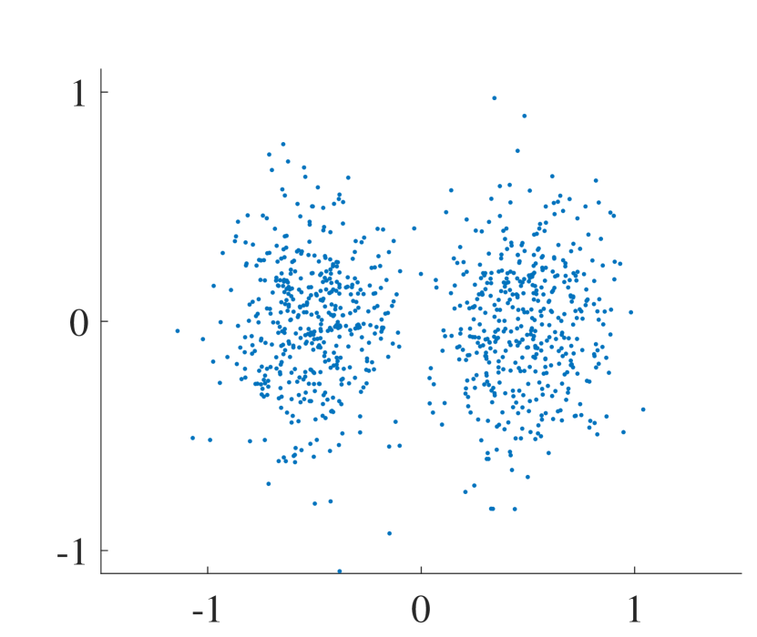
(a) Featured spikes

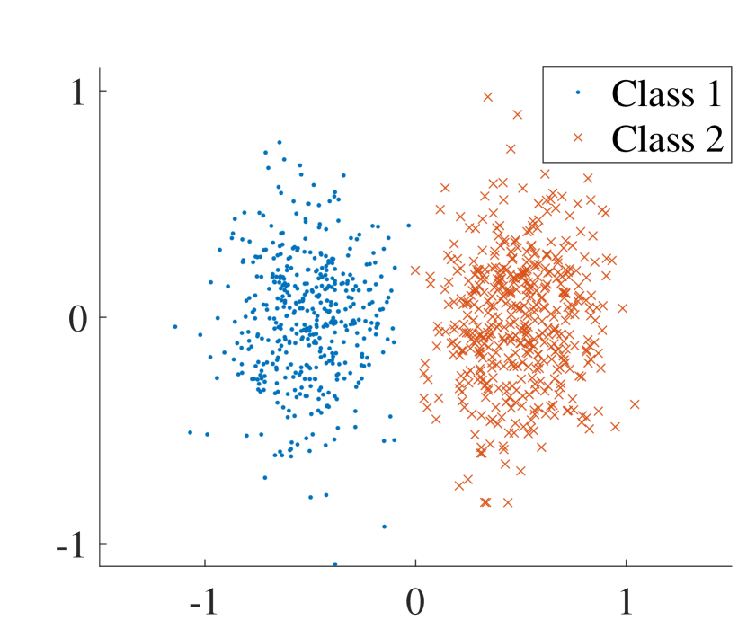
(b) K-means

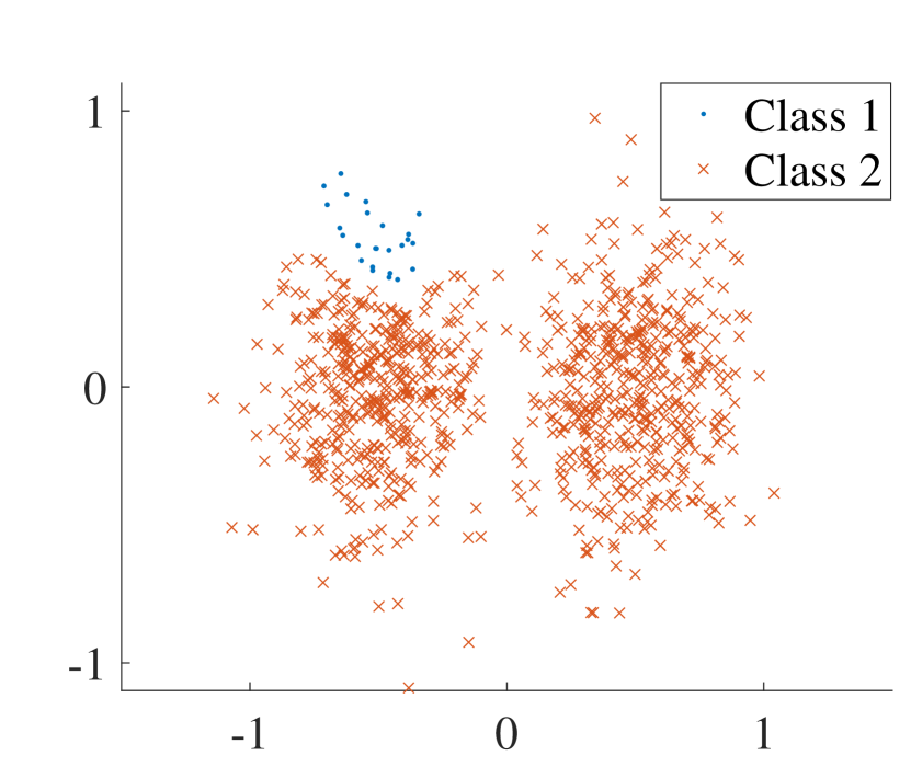
(c) Spectral clustering

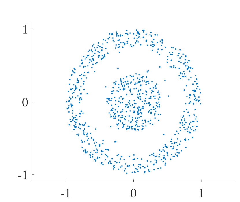
(d) Featured spikes

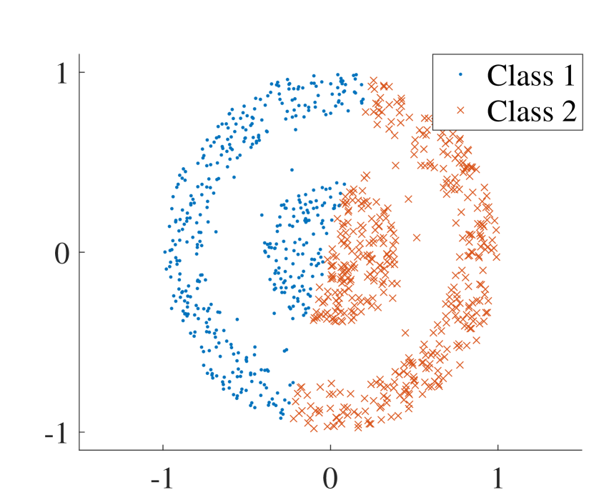
(e) K-means

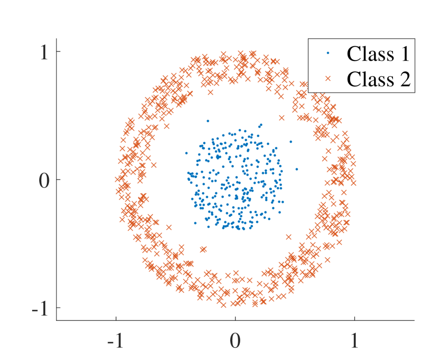
(f) Spectral clustering

Figure 1: (a) and (d) are featured spikes mapped on two dimensions which are supposed to be obtained from global-based and local-based feature extraction methods, respectively. (b) and (e) show the results from K-means while (c) and (f) from spectral clustering. For the spikes distributed in (a), K-means performs better than spectral clustering, while for (d) the conclusion is opposite.

Recently, Keshtkaran et al. [21, 18] introduced linear discriminant analysis guided by K-means (LDAKM) [22], which tried to joint LDA with KM into a coherent framework, to model the feature extraction and clustering problem in spike sorting. Subsequently, they take an additional GMM process after each KM iteration, proposing LDAGMM [18] to detect the overlapping spikes. Unfortunately, LDAKM confuses the matrix ratio trace together with trace ratio criteria in the framework, resulting in the outputs vibration or even mis-convergence [23, 24]. LDAGMM forces more different algorithms to be spliced together compared with LDAKM, which may distract the jointed model. Along with this distraction, more iteration times and computation resources are required. Therefore, both methods still suffer from unstable results.

Inspired by these efforts [21, 18], in this paper, we propose a unified optimisation model of feature extraction and clustering for spike sorting, intrinsically integrating PCA and KM, which enforces these two stages to pursue an identical criteria. In particular, by engaging alternating direction method [25], we alternatively update the extracted features and clustering results, which means the feedback from the clustering is considered in the feature extraction stage. Further, embedding K-means++ initialising and comparison updating strategies in the cluster step, the unstable problem is alleviated significantly. Finally, we derive an automatic spike sorting framework after estimating the number of neurons through existing validity indices. Our contributions are mainly three-fold,

• We propose an automatic spike sorting framework which not only keeps the time efficiency but also enjoys the high accuracy property. Moreover, the proposed method guarantees that the results are stable whether noises and/or overlapping spikes exist or not.

• We theoretically give the solution to our proposed unified model, and also prove that it can be converted into the PCA or KM like process for each alternate updating. Besides, we provide its computational complexity analysis.

• We conduct various experiments on both synthetic and real-world datasets, which verify the monotonicity of our model, rather than vibration. The efficacy and stability of our proposed method are also confirmed.

The rest of this paper is organised as follows. In section II, our automatic spike sorting framework is given in details, particularly, the newly unified feature extraction and clustering model and its solution are formulated and explained together with corresponding theoretical analysis, etc. Section III presents and discusses our experimental results. Finally, we conclude this paper in Section IV.

II Methods

In this section, the proposed automatic spike sorting framework is demonstrated in details. It includes filtering, spike detection, and the proposed unified feature extraction and clustering model integrating PCA with KM.

Filtering and amplitude threshold detection in [14] and  [26] are engaged in our framework. Note that, the particular parameters in these two steps for different datasets are, by default, assigned according to [14, 26], and we will point out these default settings in Section III as well. Thereafter, each detected spike is stored in the matrix $X\in\mathbb{R}^{d\times n}$ in the form of a column. Here, $d$ and $n$ stand for the number of variables (dimensions) and the number of observations (spikes), respectively.

II-A Theoretically Represent and Optimise PCA and KM

For easy representation, we first theoretically represent and optimise PCA and KM.

II-A1 PCA

Given a detected spike dataset $X$, the target of PCA is to construct an orthogonal linear projection matrix $W\in\mathbb{R}^{d\times m}$ so that the projected spikes lie in the $m$ linear spaces with greatest data variances. Here, $m$ is the reduced dimension.The centralisation matrix is firstly formed by [24],

$$H=I-\frac{1}{n}N\in\mathbb{R}^{n\times n},$$ (1)

where $I$ and $N$ are, respectively, the identity matrix and the all-ones matrix, in which every element is $1$. It can be checked that, $H$ is a symmetric and idempotent matrix [27], i.e., $H=H^{T}=HH^{T}$. Then, the spikes can be centred by rightly multiplying $H$, i.e., $XH$. PCA resorts to the total scatter matrix, $XH(XH)^{T}=XHX^{T}$, as,

$$\begin{split}\max_{W}&\ \ W^{T}XHX^{T}W,\\ s.t.,&\ \ W^{T}W=I.\end{split}$$ (2)

Actually, after taking the trace operation $\operatorname{tr}(\cdot)$ on the matrix, $W^{T}XHX^{T}W$, the above problem can be solved by performing eigenvalue decomposition (EVD) [27] on $XHX^{T}$. That is $XHX^{T}=W\Lambda{W}^{-1}$, where $\Lambda$ is the diagonal matrix whose diagonal entries are the corresponding eigenvalues of $XHX^{T}$. Finally, we can get the optimal value and the optimum solution, $W^{*}$, with the biggest $m$ eigenvalues in $\Lambda$ and the corresponding $m$ eigenvectors in $W$, respectively.

II-A2 KM

In KM, a label indicator matrix, $G=\left\{G_{ij}|i=1,...,n,j=1,...,c\right\}\in\mathbb{R}^{n\times c}$, is constructed by the rule that $G_{ij}=1$ if the i-$th$ spike belongs to the j-$th$ class and other elements of $G$ are $0$, where $c$ is the number of classes (i.e., neurons). Meanwhile, the centres of $c$ classes are stored as columns in the matrix $M\in\mathbb{R}^{d\times c}$. Then the entire KM clustering process can be expressed as searching for one appropriate local optima solution by performing expectation maximisation (EM) algorithm on the flowing problem [28, 29],

$$\begin{split}\min_{G,M}&\ \ \left\lVert XH-MG^{T}\right\rVert_{F}^{2},\\ s.t.,\ \ G\bm{1}_{c}=&\bm{1}_{n},\ \ G^{T}\bm{1}_{n}\succ\bm{1}_{c},\ \ G_{ij}\in\left\{0,1\right\},\end{split}$$ (3)

where $\left\lVert X\right\rVert_{F}=\left(\sum_{i=1}^{d}\sum_{j=1}^{n}|X_{ij}|^{2}\right)^{\frac{1}{2}}$ is the Frobenius norm with respect to matrix $X$, $\bm{1_{c}}\in\mathbb{R}^{c\times 1}$ is an all-ones column vector whose elements are $1$, and $X\succ Y$ indicates $X_{ij}>Y_{ij}$ with element-wise inequality.

Theorem II.1.

Let $X\in\mathbb{R}^{d\times n}$ be the input detected spikes, $\operatorname{tr}(\cdot)$ be the trace operation, and $H\in\mathbb{R}^{n\times n}$ be centralisation matrix, i.e., $H=I-\frac{1}{n}N$. Then Problem (3) is equivalent to the following one,

$$\begin{split}\min_{G}&\ \ \operatorname{tr}\left(XH(I-G(G^{T}G)^{-1}G^{T})HX^{T}\right),\\ s.t.,&\ \ G\bm{1}_{c}=\bm{1}_{n},\ \ G^{T}\bm{1}_{n}\succ\bm{1}_{c},\ \ G_{ij}\in\left\{0,1\right\}.\end{split}$$

Proof.

II.1 Denote $f(G,M)=\left\lVert XH-MG^{T}\right\rVert_{F}^{2}$. Since $\left\lVert X\right\rVert^{2}_{F}=\operatorname{tr}(XX^{T})=\operatorname{tr}(X^{T}X)$, we have,

$$f(G,M)=\operatorname{tr}\left(XHX^{T}-2MG^{T}HX^{T}+MG^{T}GM^{T}\right).$$

According to $\frac{\partial f(G,M)}{\partial M}=0$ along with $\frac{d}{dX}\operatorname{tr}\left(XY^{T}\right)=\frac{d}{dX}\operatorname{tr}\left(Y^{T}X\right)=Y$ and $\frac{d}{dX}\operatorname{tr}\left(XYX^{T}\right)=X\left(Y+Y^{T}\right)$, we can further derive,

$$M=XHG\left(G^{T}G\right)^{-1}.$$ (4)

Combining Problem (3) and Eq.(4), we get the result.∎

Theorem II.1 indicates that KM can potentially be simplified from the core EM mechanism with iteratively updating two variables to the problem with only one variable needed to be solved.

II-B Unify PCA and KM for Spike Feature Extraction and Clustering

In the conventional spike sorting procedure, KM is performed after doing PCA on the centralised data matrix, $XH$, for dimension reduction. That is to say, $W^{T}XH$ is actually fed into KM. In addition, PCA is a maximisation problem for pursing the single variable, $W$, and KM has the potential to be transformed into a minimisation problem for pursing the single-variable, $G$. By employing Theorem II.1 and a trace operation on the ratio of matrix [30], we can integrate PCA and KM into one optimisation problem as follows,

$$\begin{split}\max_{G,W}&\ \ \operatorname{tr}\left\{\frac{W^{T}XHX^{T}W}{W^{T}XH(I-G(G^{T}G)^{-1}G^{T})HX^{T}W}\right\},\\ s.t.,&\ \ G\bm{1}_{c}=\bm{1}_{n},\ \ G^{T}\bm{1}_{n}\succ\bm{1}_{c},\ \ G_{ij}\in\left\{0,1\right\},\\ &\ \ W^{T}W=I.\end{split}$$ (5)

We engage the alternating direction method [25] with two-updating steps to solve the above problem, which guarantees to converge.

II-B1 Update G

When updating $G$, we ignore the constraint associated with $W$ and convert the maximisation problem to a minimisation one. Then Problem (5) is converted to,

$$\begin{split}\min_{G}&\ \ \operatorname{tr}\left\{\frac{W^{T}XH(I-G(G^{T}G)^{-1}G^{T})HX^{T}W}{W^{T}XHX^{T}W}\right\},\\ s.t.,&\ \ G\bm{1}_{c}=\bm{1}_{n},\ \ G^{T}\bm{1}_{n}\succ\bm{1}_{c},\ \ G_{ij}\in\left\{0,1\right\}.\end{split}$$ (6)

According to Theorem II.1, solving the above problem equals to performing the following KM-like procedure,

$$\begin{split}\min_{G}&\ \ \left\lVert\left(W^{T}XHX^{T}W\right)^{-\frac{1}{2}}W^{T}XH-MG^{T}\right\rVert_{F}^{2},\\ s.t.,&\ \ G\bm{1}_{c}=\bm{1}_{n},\ \ G^{T}\bm{1}_{n}\succ\bm{1}_{c},\ \ G_{ij}\in\left\{0,1\right\},\end{split}$$ (7)

where $M=\left(W^{T}XHX^{T}W\right)^{-\frac{1}{2}}W^{T}XHG\left(G^{T}G\right)^{-1}$. To get a better optimum, we use two strategies as follows,

• Different from randomly initialising the class centres, we make use of the well-known K-means++ [31] initialisation strategy.

• To ameliorate the local optimum problem, we employ a comparison updating rule [27] detailed as follows.

Updating Rule: We begin by defining that,

$$g(G,M)=\left\lVert\left(W^{T}XHX^{T}W\right)^{-\frac{1}{2}}W^{T}XH-MG^{T}\right\rVert_{F}^{2}.$$

Suppose that we obtain the solutions to Problem (5), $W_{t}^{*}$ and $G_{t}^{*}$ along with the corresponding $M_{t}^{*}$, after the $t$-th iteration. Before updating $G$ at the $(t+1)$-th iteration, we firstly initialise $\left\{M_{t+1}^{1},M_{t+1}^{2},...,M_{t+1}^{a}\right\}$ by using K-means++ strategy, and calculate the corresponding $\left\{G_{t+1}^{1},G_{t+1}^{2},...,G_{t+1}^{a}\right\}$. Here, $a$ denotes the number of initialisations, which is fixed to be $10$ in our model. Then we update $G$ with the following criteria,

$$G_{t+1}^{*}=\begin{cases}G_{t+1}^{i},&\ {\rm if}\ g(G_{t+1}^{i},M_{t+1}^{i})<g(G_{t}^{*},M_{t}^{*});\\ G_{t+1}^{\prime},&\ \ {\rm otherwise},\end{cases}$$ (8)

where $i=1,2,...,a$, and $G_{t+1}^{\prime}$ is defined as the solution to following problem,

$$\begin{split}\min_{G}&\ \ \left\lVert\left({W_{t}^{*}}^{T}XHX^{T}{W_{t}^{*}}\right)^{-\frac{1}{2}}{W_{t}^{*}}^{T}XH-M_{t}^{*}G^{T}\right\rVert_{F}^{2},\\ s.t.,&\ \ G\bm{1}_{c}=\bm{1}_{n},\ \ G^{T}\bm{1}_{n}\succ\bm{1}_{c},\ \ G_{ij}\in\left\{0,1\right\}.\end{split}$$ (9)

II-B2 Update W

When updating $W$, viewing $G$ as a constant, Problem (5) can be recast as,

$$\begin{split}\max_{W}&\ \ \operatorname{tr}\left\{\frac{W^{T}XHX^{T}W}{W^{T}XH(I-G(G^{T}G)^{-1}G^{T})HX^{T}W}\right\},\\ s.t.,&\ \ W^{T}W=I.\end{split}$$ (10)

The above problem is a convex optimisation, which has a closed-form solution. It can be solved by the following proposition.

Proposition 1.

The optimal solution to (10) can be derived by picking up $m$ generalised eigenvectors corresponding to the $m$ largest generalised eigenvalues of the decomposition as follows,

$$(XHX^{T})W=\left[XH(I-G(G^{T}G)^{-1}G^{T})HX^{T}\right]W\Lambda$$ (11)

The proofs of this proposition are provided in Appendix A.

Finally, the whole solving algorithm of our proposed model is summarised in Alg.1.

Algorithm 1 The algorithm for solving Problem (5)

0:  The detected spikes $X\in\mathbb{R}^{d\times n}$, the number of neurons $c$.

0:  Transformation matrix $W^{*}\in\mathbb{R}^{d\times m}$, the allocation results of spikes $G^{*}\in\mathbb{R}^{n\times c}$.

1:  Initialise $m=c-1$, $t=1$; Define $H\in\mathbb{R}^{n\times n}$, $W^{(0)}\in\mathbb{R}^{d\times m}$, and $G^{(0)}\in\mathbb{R}^{n\times c}$ according to Eqs.(1), (2), and (3), respectively.

2:   Update $W_{t}$ according to Proposition 1.

3:  Update $G_{t}$ according to Eq.(8).

4:  Quit the loop if $G_{t}=G_{t-1}$, otherwise, $t=t+1$ and go back to step 2.

5:  Return $G^{*}=G_{t}$ and $W^{*}=W_{t}$.

II-C Other Descriptions of the Unified Model

In this subsection, the computational complexity of the proposed model is analysed, and schemes of automatically estimating of the number of neurons and determining the dimension of the reduced feature are presented.

II-C1 Analysing the Computational Complexity

The computational complexity of our proposed model mainly consists of three parts: the calculation of $W^{T}XHXW$ when $W$ is known; Using KM to solve submodel (9); Using generalised EVD to solve submodel (11). In fact, by reusing the constructed $XHX\in\mathbb{R}^{d\times d}$, the time complexity of constructing $W^{T}XHXW$ is $O(d^{2}m+m^{2}d)$. The computational complexity of KM is $O(nmc)$ [29], while that of the generalised EVD is $O(d^{2}n)$ [27]. Here, $d$, $n$, $m$, and $c$ denote the original dimensions of the spike, the total number of spikes, the reduced dimensions of the spike, and the number of spike’s categories, respectively. Therefore, the total complexity is $O(b(d^{2}m+m^{2}d+nmc+d^{2}n))$. Generally, it can be further simplified to $O(bd^{2}n)$, which is linear to the number of spikes, since $n\gg d>m,c$ and $b\approx 10$ hold in the single electrode or tetrode extracellular recorded signal.

II-C2 Automatically Estimating the Number of Neurons

Although many spike sorting methods determine the number of neurons by manually specifying or graphically merging and decomposing clusters [17, 26, 32], integrating existing estimation methods into the model can reduce a lot of unnecessary human intervention [21]. To this end, we integrate the estimation of the number of neurons after the model initialisation and before the main iterative optimisation. Within a range of the number of neurons in initial settings, the spike sorting algorithm is pre-run to obtain a series of corresponding index values, and then one reasonable number of neurons is picked up based on the best index value [12, 33]. Two clustering validity indices, Calinski Harabasz [34] and gap [15], are employed in this paper.

II-C3 Automatically Determining the Number of Features

To efficiently reduce the time consumption and further free human intervention, in our method, automatically determining the dimensions of spikes is adopted. Specifically, $m_{0}$, as the initially reduced dimensions, only affects the estimation of the number of neurons. After estimating the number of neurons $\tilde{c}$, $m=\tilde{c}-1$ is recommended, where $m$ denotes the dimension of the spike in iteration process. This strategy not only reduces computational complexity in each iteration but avoids the singularity problem [23] in EVD.

Finally, our proposed automatic spike sorting procedure is summarised in Alg.2.

Algorithm 2 Proposed automatic spike sorting procedure

0:  The recorded spike signal; The initial reduced dimension $m_{0}$.

0:  Transformation matrix $W^{*}\in\mathbb{R}^{d\times m}$, the allocation results of spikes $G^{*}\in\mathbb{R}^{n\times\tilde{c}}$, and the estimated number of neurons $\tilde{c}$.

1:  Filter and detect the recorded signal to get the spikes signal matrix $X\in\mathbb{R}^{d\times n}$.

2:  Initialise $t=1$; Define $H\in\mathbb{R}^{n\times n}$ and $W^{(0)}\in\mathbb{R}^{d\times m_{0}}$ by solving (1) and (2), respectively.

3:  Estimate the best number of neurons $\tilde{c}$ and $G^{(0)}\in\mathbb{R}^{n\times\tilde{c}}$ simultaneously by solving (3) with $W_{0}$ and Calinski Harabasz [34] or gap [15].

4:   Update $W^{(t)}$ according to Proposition 1.

5:  Update $G^{{(t)}}$ according to (8).

6:  Quit the loop if $G^{(t)}=G^{(t-1)}$, otherwise, $t=t+1$ and go back to step 4.

7:  Return $G^{*}=G^{(t)}$, $W^{*}=W^{(t)}$ and $\tilde{c}$.

III Experiments

The proposed automatic spike sorting method is evaluated on both several well-known simulated datasets and the real tetrode-recorded dataset. Further, we compared it with several related state-of-the-art spike sorting methods on different evaluation criteria, including neurons estimation, accuracy, time consumption, stability, etc. All codes of our experiments are implemented in MATLAB R2020a, which is run on a personal computer with Intel Core i7-8750H 2.20 GHz CPU, 32G RAM).

III-A Experimental Datasets and Evaluation Criteria

Four challenging synthetic neural datasets in Wave_clus [14, 35], which own the ground truths, are used in our simulations. They are Easy1_noise*, Easy2_noise*, Difficult1_noise*, and Difficult2_noise*, in which the asterisk stands for the embedded noise standard deviation (i.e., noise level) with respect to the main waveforms. Here, the waveforms were issued by three neurons in neocortex and basal ganglia [35], and the noise was mimicked by randomly selecting the real recorded signal with different amplitudes from different neurons [14]. Note that, ‘Easy’ reflects that the used waveforms are easy to distinct (i.e., they are different from each other) and vice versa for the ‘Difficult’. Besides, the noise level of ‘Easy1’ is ranging from 0.05 to 0.4 with the step length 0.05 while those of the rest three datasets are in [0.05, 0.2].

We also engaged the publicly available vivo dataset, HC1 [3] in our real-world experiment. HC1 was recorded from the anesthetized rat hippocampus using an extracellular tetrode, with which one extra intracellular electrode was implanted to a single neuron to obtain its actual spike times (refer to ground truth) for evaluation [36, 26].

To take the best detected spike in simulation datasets and avoid errors from detection, we pick up spikes based on the ground truth for Wave_clus. Then, with the detected spike matrix $X$, we evaluated the performance of determining the number of neurons, clustering accuracy, time consumption, etc. Especially, to reflect the stability, we conducted $20$ independent trials, which resulted in corresponding means and their standard deviations. As for the real-world dataset, HC1, the F1 related criteria, false negative rate (FNR, or called as Miss rate) and false positive rate (FPR), are used. Here, the false negative represents that the predicted cluster is negative but the real class is true, while the false positive means the predicted cluster is positive but the real class is false. FNR and FPR are reasonable enough to reflect the clustering results, and lower values for both of them mean better performances [26, 18].

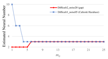
Figure 2: The relationship between the initial number of features $m_{0}$, and the estimated number of neurons $\tilde{c}$ on two datasets.

III-B Experiments on Synthetic Dataset - “Wave_clus”

Same as the original works [14, 35], “Wave_clus” was filtered with passband located at $300-6,000$ Hz firstly. But different from the default configuration using amplitude thresholds to detect spikes, we directly extracted those spikes by using a $64$ sample-length window from the known spike time in ground truths. This facilitates to get consistent spike datasets to perform fair comparison with different methods.

III-B1 Determination of the Number of Neurons

TABLE I: The number of estimated neurons using various automatic spike sorting methods on Wave_clus datasets with (without) overlapping spikes.

DS	NL	With Overlapping Spikes (Without)
		A	B	C	D	E	P1	P2
Easy1	05 10 15 20 25 30 35 40	2(3) 3(3) 8(2) 3(2) 2(7) 3(2) 3(3) 4(3)	2(10) 6(9) 2(4) 3(7) 2(2) 8(3) 4(2) 2(2)	2(4) 2(4) 2(3) 2(5) 2(3) 2(5) 2(5) 2(4)	2(3) 2(5) 2(4) 2(5) 2(4) 2(5) 4(5) 2(4)	3 3 3 3 6 3 4 3	3(3) 3(3) 3(3) 3(3) 3(3) 3(3) 3(3) 3(3)	3(5) 3(3) 3(3) 3(3) 3(3) 3(3) 3(3) 3(3)
Easy2	05 10 15 20	7(4) 3(3) 8(2) 3(2)	3(7) 7(10) 6(6) 9(10)	2(5) 2(3) 3(3) 2(3)	2(2) 2(3) 2(3) 2(4)	6 3 3 3	3(3) 2(3) 2(2) 2(2)	3(5) 3(3) 3(3) 3(3)
Difficult1	05 10 15 20	6(7) 3(2) 2(2) 4(3)	6(10) 2(3) 2(3) 2(2)	2(4) 2(4) 2(6) 2(5)	2(4) 2(6) 2(4) 3(7)	4 3 3 4	3(6) 3(3) 3(3) 3(3)	8(6) 3(3) 2(2) 2(2)
Difficult2	05 10 15 20	8(3) 9(3) 9(3) 8(4)	3(8) 3(6) 2(10) 2(9)	2(4) 2(5) 2(3) 3(4)	2(3) 2(4) 2(3) 2(4)	4 3 4 3	3(3) 2(3) 2(2) 2(2)	3(3) 3(6) 3(3) 2(2)
Total Hit		8(7)	4(3)	2(6)	2(5)	13	14(15)	16(13)

• DS and NL are the names and the noise levels of datasets, respectively. A, B, C, D, and E stand for the automatic spike sorting frameworks of LE-KM [16], LPP-SCK [15], LDAKM [21], LDAGMM [18], and the Wave_clu [14] baseline, respectively. P1 and P2 refer to our proposed model with Calinski Harabasz [34] and gap [15] index for estimating the number of neurons.

TABLE II: The average accuracy (± its standard deviation) and average processing time (± its standard deviation) of various spike sorting algorithms after repeating 20 times for each dataset without overlapping spikes. Here the number of classes is fixed to be $3$ and the reduced dimensions of spikes are $2$.

DS	NL	SN	PCA-KM	PCA-SCK	LE-KM	LPP-SCK	GF-KM	GF-SCK	LDAKM	Proposed
Easy1	05 10 15 20 25 30 35 40	2729 2753 2693 2678 2586 2629 2702 2645	100.00±0.00 100.00±0.00 100.00±0.00 99.93±0.00 99.81±0.00 99.20±0.00 97.11±0.00 94.33±0.00	84.57±15.84 91.27±9.06 85.65±14.98 88.51±11.87 89.24±9.84 98.91±1.05 97.32±0.54 94.66±0.24	100.00±0.00 98.95±0.00 93.13±0.00 87.04±0.00 87.39±0.00 84.33±0.0 79.24±0.00 74.43±0.03	83.02±12.92 88.34±8.69 80.75±8.49 80.30±8.01 85.53±1.26 77.60±1.32 69.70±9.85 64.07±8.25	100.00±0.00 100.00±0.00 100.00±0.00 100.00±0.00 100.00±0.00 100.00±0.00 99.96±0.00 97.58±0.00	84.30±16.07 78.62±18.08 88.44±15.01 93.90±8.57 85.33±12.21 88.93±12.30 82.90±19.81 92.57±11.60	100.00±0.00 100.00±0.00 100.00±0.00 100.00±0.00 100.00±0.00 100.00±0.00 99.99±0.01 99.99±0.02	100.00±0.00 100.00±0.00 100.00±0.00 100.00±0.00 100.00±0.00 100.00±0.00 100.00±0.00 100.00±0.00
Easy2	05 10 15 20	2619 2694 2648 2715	100.00±0.00 99.07±0.00 92.86±0.00 85.12±0.00	81.12±15.67 87.15±9.69 78.45±13.84 75.93±11.63	100.00±0.00 100.00±0.00 100.00±0.00 95.54±0.00	83.44±16.44 89.44±12.66 85.03±17.43 83.65±14.84	100.00±0.00 100.00±0.00 100.00±0.00 95.17±0.00	87.49±12.59 89.61±12.36 90.59±15.59 86.24±9.28	98.60±6.25 100.00±0.00 100.00±0.00 100.00±0.00	100.00±0.00 100.00±0.00 100.00±0.00 100.00±0.00
Difficult1	05 10 15 20	2616 2638 2660 2624	97.13±0.00 88.21±0.00 70.23±0.00 56.59±0.02	93.80±2.78 86.81±0.66 53.00±6.77 50.26±4.30	100.00±0.00 88.07±0.53 81.99±0.03 60.94±0.00	81.61±19.54 98.35±3.77 80.93±0.51 53.65±4.20	100.00±0.00 99.70±0.00 81.78±0.05 58.96±0.00	83.93±16.49 93.06±13.44 81.30±0.61 56.71±3.07	100.00±0.00 99.12±3.94 98.98±4.54 98.86±4.54	100.00±0.00 100.00±0.00 100.00±0.00 100.00±0.00
Difficult2	05 10 15 20	2535 2742 2631 2716	100.00±0.00 99.85±0.00 92.25±0.00 74.11±0.01	81.30±15.03 95.07±7.54 82.63±10.31 73.77±0.28	100.00±0.00 100.00±0.00 100.00±0.00 100.00±0.00	85.06±16.57 88.15±17.65 87.53±11.63 81.07±14.72	100.00±0.00 100.00±0.00 100.00±0.00 100.00±0.00	84.84±19.04 86.33±14.61 91.17±12.44 84.29±14.31	100.00±0.00 100.00±0.00 98.51±6.67 100.00±0.00	100.00±0.00 100.00±0.00 100.00±0.00 100.00±0.00
Average Time / s			0.03±0.01	0.22±0.01	0.20±0.03	0.38±0.01	0.22±0.03	0.43±0.01	0.63±0.16	0.17±0.14

Four automatic spike sorting methods (LE-KM [16], LPP-SCK [15], LDAKM [21], LDAGMM [18]) are compared in estimating the number of neurons on the whole datasets with/without overlapping spikes. Here, SCK is short for landmark-based spectral clustering using KM for landmark-selection [37]. Additionally, the baseline method [14] performed on Wave_clus was contrasted on the whole datasets only with overlapping spikes. It should be noted that, since several works [38, 39] have emphasised that the number of neurons detected by extracellular electrodes should lie between 8 and 10, in our experiments a more reasonable initial range of the estimated number of neurons is set to [2, 10]. The reduced dimension, $m_{0}$, at the initialisation stage in our method is assigned to $3$, and the parameters for all compared automatic methods are set by default. Actually, different values of $m_{0}$ result in various numbers of estimated neurons but it tends to be stable as $m_{0}$ increases. Fig.2 shows the inference of $m_{0}$ to the estimated number of neurons on two datasets without overlapping spikes. Since other datasets have similar results, they are omitted here.

The results of different methods in estimating the number of neurons are presented in Table I. Note that the distinct spikes in each dataset are generated by 3 neurons.The number in parentheses indicates that the results are deduced on the dataset without the influence from overlapping spikes. It can be seen from Table I that the results of our proposed method reach the baseline level and relatively outperform those of LE-KM, LPP-SCK, LDAKM, and LDAGMM. The main reasons include, 1) the estimation results from LE-KM and LPP-SCK are sensitive to the reduced dimensions of features. 2) For LDAKM and LDAGMM, the estimation process is mixed in the iteration optimisation, making the results susceptible to the model’s random initial point and vibrant iteration. 3) Our proposed method integrated with Calinski Harabasz [34] or gap [15] index succeed largely with the stable input of the estimation from PCA initialisation as shown in Eq.(2).

III-B2 Overall Accuracy and Time Consumption

Secondly, the overall accuracy and time consumption of various spike sorting methods are compared. The state-of-the-art spike feature extraction methods, PCA [11], LE [16], LPP [15], GF [17], LDA [21, 18], along with three automatic spike sorting schemes, LE-KM [16], LPP-SCK [15], LDAKM [21, 18] are compared. Noted that the results of LDAGMM, which are similar to those of LDAKM, are not shown here due to the space limitation. Further, we also combined either PCA or GF with KM and SCK as spike sorting methods for more general comparisons. For the sake of fair comparison, the number of neurons and the reduced dimension for each method are assigned as $3$ and $2$, respectively.

TABLE III: The average accuracy (± its standard deviation) and average processing time (± its standard deviation) of various spike sorting algorithms after repeating 20 times for each dataset. Here the number of neurons and the reduced dimension are fixed with $3$ and $2$, respectively.

DS	NL	SN	PCA-KM	PCA-SCK	LE-KM	LPP-SCK	GF-KM	GF-SCK	LDAKM	Proposed (Time)
Easy1	05 10 15 20 25 30 35 40	3514 3522 3477 3474 3298 3475 3534 3386	99.23±0.00 99.40±0.00 99.19±0.00 99.11±0.00 99.00±0.00 98.04±0.00 95.90±0.01 92.98±0.01	99.24±0.08 99.44±0.03 99.18±0.03 99.02±0.08 98.99±0.08 98.22±0.13 96.28±0.12 92.60±0.40	67.59±0.05 98.38±0.00 96.87±0.00 94.67±0.00 90.72±0.00 86.42±0.00 80.48±0.00 73.72±0.00	96.20±0.71 97.91±0.41 94.93±0.89 89.04±3.29 81.35±3.42 71.43±3.29 79.55±0.47 70.06±0.61	99.35±0.00 99.55±0.00 99.65±0.00 99.77±0.00 99.42±0.00 99.45±0.00 99.35±0.00 98.49±0.00	99.31±0.11 99.55±0.11 99.62±0.03 99.57±0.04 90.50±14.54 99.70±0.04 99.61±0.02 99.53±0.15	97.85±7.30 99.66±0.14 99.65±0.09 99.77±0.06 99.64±0.06 99.60±0.02 99.55±0.05 99.69±0.07	99.52±0.00 (0.24) 99.77±0.00 (0.24) 99.68±0.00 (0.25) 99.80±0.00 (0.24) 99.76±0.00 (0.23) 99.60±0.00 (0.39) 99.63±0.00 (0.25) 99.79±0.00 (0.29)
Easy2	05 10 15 20	3410 3520 3411 3526	98.09±0.00 95.94±0.00 90.00±0.00 82.99±0.01	97.82±0.16 95.49±0.63 87.45±0.84 82.68±0.84	98.80±0.00 99.26±0.00 98.59±0.00 93.85±0.00	98.57±0.04 99.18±0.02 98.59±0.11 93.81±0.84	99.12±0.00 99.74±0.00 99.38±0.00 91.98±0.01	99.06±0.18 99.75±0.03 99.36±0.15 91.06±0.91	96.97±8.27 98.52±5.49 98.37±5.71 99.60±0.06	99.74±0.00 (0.30) 99.77±0.00 (0.40) 99.79±0.00 (0.33) 99.74±0.00 (0.41)
Difficult1	05 10 15 20	3383 3448 3472 3414	95.71±0.00 86.06±0.01 68.32±0.05 55.58±0.03	94.94±1.20 85.48±0.78 50.52±4.08 47.27±3.05	97.37±0.00 97.51±0.00 76.37±0.04 48.22±0.19	98.44±0.09 97.35±0.47 71.61±7.47 45.97±2.65	97.87±0.00 69.37±0.00 79.52±0.01 47.51±0.00	97.77±0.12 96.33±2.34 77.07±4.94 48.54±3.73	95.57±10.08 96.52±6.86 97.53±2.15 98.42±0.08	99.35±0.00 (0.39) 99.07±0.00 (0.41) 98.96±0.01 (0.56) 98.79±0.02 (1.01)
Difficult2	05 10 15 20	3364 3462 3440 3493	98.54±0.00 97.66±0.00 86.65±0.01 68.31±0.00	98.46±0.03 97.76±0.05 86.28±0.50 67.67±0.81	99.67±0.00 99.77±0.00 99.62±0.07 99.63±0.00	99.67±0.07 99.76±0.02 99.49±0.03 99.56±0.03	99.67±0.00 99.62±0.00 99.68±0.00 99.74±0.00	99.66±0.06 99.71±0.06 99.63±0.05 99.73±0.03	99.71±0.04 99.86±0.03 99.76±0.02 99.85±0.06	99.79±0.00 (0.45) 99.86±0.00 (0.31) 99.80±0.00 (0.32) 99.89±0.00 (1.10)
Average Time / s			0.04±0.02	0.27±0.01	0.31±0.03	0.52±0.02	0.36±0.02	0.62±0.03	0.64±0.14	0.41±0.24

Specifically, in LE-KM, the number of nearest neighbours is, by default, set to be $12$, however, the number of times to randomly repeat KM is not specified, and we set it to be $10$ (it is equal to the number of K-means++ initialisations in our proposed method as mentioned in subsection II-B1). Besides, the points of landmarks in SCK and the number of neighbours for each sample in LPP are, by default, fixed to be $1000$ and $5$, respectively. As for LDAKM, the open-source code is publicly accessed [40], while the configurations of our proposed method are detailed in Alg.1 . Note that, $20$ independent times are performed in each method on each dataset and the final average results along with its standard deviation are recorded. In our experiments, whether the overlapping spikes exist or not in the datasets is compared.

As shown in Table II, without overlapping spikes, nearly all methods could get acceptable results on datasets with small noise levels. But when the noise level increases, it seems that only the model-based method (i.e., LDAKM and our proposed method) can maintain high accuracy, while other combined feature extraction and clustering in sequence methods failed. On the other hand, the results of methods combined with SCK (i.e., PCA-SCK, LPP-SCK, GF-SCK) and LDAKM are not stable. For example, the standard deviations of the average accuracy for LDAKM are around $5\%$ and those for the SCK-based methods are even more than $15\%$ in the datasets of Easy2_noise05, Difficult1_noise10, etc. The standard deviations of the methods combined with KM (i.e., PCA-KM, LE-KM, GF-KM) are comparable with setting a sufficient number of initialisation, however, the average accuracies are not satisfactory. On the contrary, by initialising with K-means++ strategy and updating with comparison rule whose details are shown in section II-B1, our proposed method obtains the near-perfect accuracies. At the same time, the processing time is also less than others. What’s more interesting is that by calculating the standard deviation of the processing time, the minimum processing time of our proposed method is equal to the simple combined method, PCA-KM. This means the proposed method can automatically adjust the processing time according to the complexity of the dataset. These findings are also consistent with the presence of overlapping spikes as shown in Table III, in which the exact processing time of our method on each dataset is manifested.

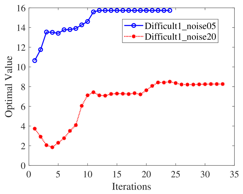
(a) LDAKM

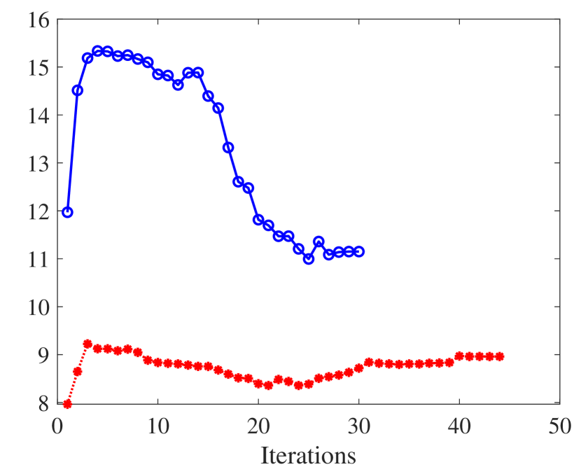
(b) LDAGMM

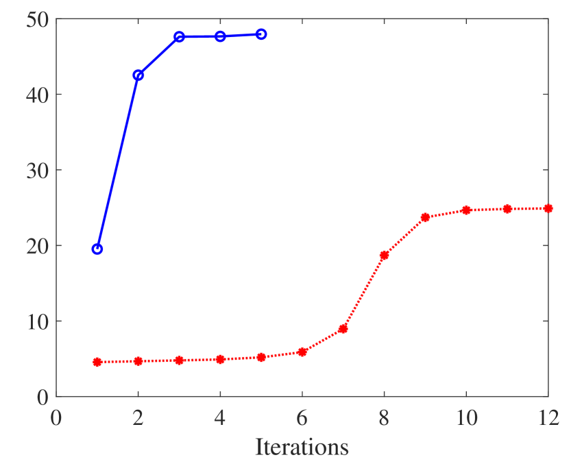
(c) Proposed

Figure 3: The optimal value versus the times of iteration on two datasets of (a) LDAKM, (b) LDAGMM, and (c) our proposed method.

III-B3 Monotonicity Experiments

Finally, in order to verify the monotonicity of our proposed method, we graph the model objective value versus the times of iteration. The results on Difficult1_noiseo5 and Difficult1_noise20 are illustrated while other datasets with similar results are ignored. At the same time, we also compared the model-based spike sorting methods, LDAKM and LDAGMM. As shown in Fig.3(c), the proposed method always iterates towards the increasing objective values and converges after about $10$ iterations. Although LDAKM has a trend of increasing the objective values overall, its optimal value is not always increasing, since the objective function of the two-step solution for LDAKM is different [24]. Furthermore, LDAGMM adds GMM operations after each KM [18], making its objective value even iterate toward a decreasing direction. LDAKM and LDAGMM need more iterations (Fig.3(a) and Fig.3(b)), and also more computational resources (Tables II and III).

III-C Experiment on Real-world Dataset - “HC1”

In this section, the real-world dataset, HC1 [3], is used and four automatic spike sorting methods, LE-KM [16], LPP-SCK [15], LDAKM [21], LDAGMM [18], are compared. Similar as [26, 18], we firstly filter the raw recorded signal using a highpass Butterworth filter at 250 Hz with order 50. Then, spikes were identified by exceeding a threshold that is assigned by [26]. For more detailed preprocessing about the spike filtering and detection, please refer to the open source [41]. Actually, after these preprocessings, all the ground truth spikes recorded by the intracellular electrode are detected. Then the spikes from the tetrode are concatenated into a vector for further automatic sorting. Finally, according to the existing ground truth intracellularly recorded from one neuron, we can obtain the corresponding FPR and FNR.

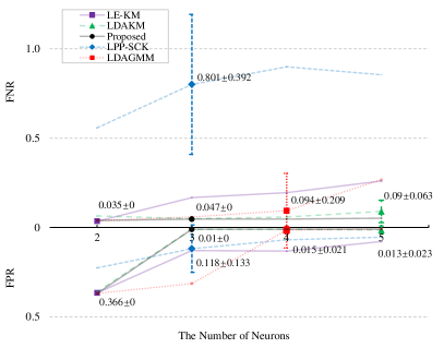
Figure 4: FPR and FNR obtained by several automatic spike sorting methods, i.e., LE-KM, LDAKM, LPP-SCK, LDAGMM and our proposed one on the HC1 datasets. Here, results with the estimated neurons from 2 to 5 are included, and among them, the bold dots indicate the actual estimated results (along with their standard deviation) for each method.

In Figure 4, the results of five automatic spike sorting methods are shown when the estimated neurons ranges from $2$ to $5$. Among them, the actual estimated results are emphasised with bold dots and their numerical values are also accompanied. On one hand, it is easy to find that the results of LDAKM, LPP-SCK, and LDAGMM are unstable, especially the standard deviation of the FNR of LPP-SCK reaches $39.2\%$. On the other hand, LDAKM and our proposed method get better results for different estimated neurons compared with LE-KM, LPP-SCK and LDAGMM, although the actual estimated number is different between them (the proposed method is $3$ while LDAKM is $5$).

In addition to FPR and FNR, we also showed the mean waveforms of ground truth and the distribution of spikes obtained by different methods. Specifically, assuming the estimated number of neurons is $\tilde{c}$, when $\tilde{c}\leq 3$, the graphical dimension is $\tilde{c}-1$ while when $\tilde{c}>3$, the dimension is $3$. Meanwhile, the average waveform from each class of spike is also shown under the corresponding panel. As we can see from Fig.5, the number of neurons and their waveforms obtained by various methods are different. Relatively speaking, the results of our proposed method are better since the graphical results show three distinctly different clusters and waveforms. In contrast, the results of LE-KM (Fig.5(b)) and LPP-LCK (Fig.5(c)) do not separate the spikes reasonably. With further analysing the average waveforms, we can see that the second (red) waveforms from our proposed method are more consistent with the ground truth compared with the third (yellow) waveforms from LDAKM and the second (red) waveforms from LDAGMM. Besides, it appears that the first (blue) and second (red), fourth (purple) and fifth (green) waveforms of LDAKM (Fig.5(d)) are very similar, and we prefer to merge them together. Similarly, for LDAGMM (Fig.5(e)), the third (yellow) and fourth (purple) waveforms are also very similar.

In summary, our proposed method exhibits excellent accuracy and stability in both synthetic and real-world datasets.

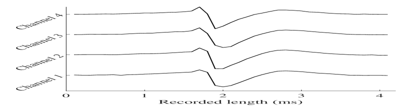
(a) Ground truth

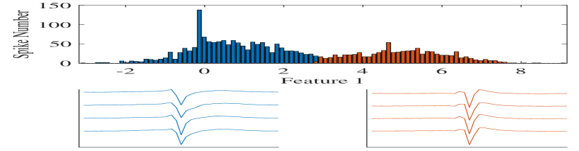
(b) LE-KM

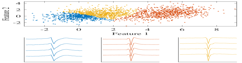
(c) LPP-LCK

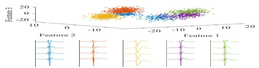
(d) LDAKM

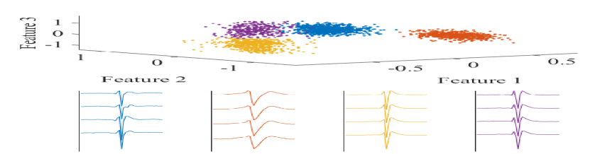
(e) LDAGMM

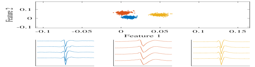
(f) Proposed

Figure 5: The mean waveform of ground truth is shown in (a), along with the low-dimensional distributions of spikes and their mean waveforms of each cluster from several automatic spike sorting schemes: (b) LE-KM, (c) LPP-LCK, (d) LDAKM, (e) LDAGMM, and (f) our proposed method.

IV Conclusions

This paper studied a optimisation problem for spike sorting which unified the feature extraction and clustering. It was basically solved in an integrated framework with PCA and K-means. The computational complexity of this model is linear to the number of spikes, which is less than existing methods. In particular, we proposed an efficient and effective automatic spike sorting method after integrating existing strategies to estimate the number of neurons. The yielded satisfactory and stable results on both synthetic and real datasets verified the efficacy of our proposed method.

Appendix A Proofs

Proof (of Proposition 1): Let $S_{1}=XHX^{T}$ and $S_{2}=XH\left(I-G\left(G^{T}G\right)^{-1}G^{T}\right)HX^{T}$, we can simplify (10) as,

$$\begin{split}\max_{W}&\ \ \operatorname{tr}\left\{\frac{W^{T}S_{1}W}{W^{T}S_{2}W}\right\},\\ s.t.,&\ \ W^{T}W=I.\end{split}$$ (A.1)

Because $S_{1}$ and $S_{2}$ are symmetric matrix, there exists a $d\times d$ nonsingular square matrix $A$ so that,

$$\begin{split}A^{T}W^{T}S_{2}WA=I_{d},\ \ \mathrm{and}\ \ A^{T}W^{T}S_{1}WA=M_{d},\end{split}$$ (A.2)

where $M_{d}$ is a $d\times d$ diagonalised matrix. According to (B), (B.4), (A.1), and (A.2), we have,

$$S_{2}^{-1}S_{1}W =W\left(W^{T}S_{2}W\right)^{-1}\left(W^{T}S_{1}W\right)$$

$$=W\left(\left(A^{T}\right)^{-1}I_{d}A^{-1}\right)^{-1}\left(\left(A^{T}\right)^{-1}M_{d}A^{-1}\right)$$

$$=WAM_{d}A^{-1},$$

that is, $S_{2}^{-1}S_{1}WA=WAM_{d}$. Besides,

$$\begin{split}&\operatorname{tr}\left\{\frac{W^{T}S_{1}W}{W^{T}S_{2}W}\right\}\\ &=\operatorname{tr}\left\{\left(A^{T}W^{T}S_{2}WA\right)^{-1}\left(A^{T}W^{T}S_{1}WA\right)\right\},\\ &=\operatorname{tr}\left\{\frac{A^{T}W^{T}S_{1}WA}{A^{T}W^{T}S_{2}WA}\right\}=\operatorname{tr}\left\{M_{d}\right\}.\end{split}$$

Therefore, the optimal value of (A.1) can be determined by the $m$ largest eigenvalues of $M_{d}$. Also the corresponding eigenvectors in $WA$ are the optimal solution of (A.1). Certainly such eigenvalues and eigenvectors could be deduced from generalised eigenvalue decomposition on $S_{2}^{-1}S_{1}$, so they also satisfy the decomposition (11) and Proposition 1 is proved.

Appendix B Main mathematical Properties

The following equations are used in the Appendix A.

$$\frac{d}{dX}\operatorname{tr}\left\{X^{T}YX\right\}=\left(Y+Y^{T}\right)X$$ (B.1)

$$\frac{d}{dX}\operatorname{tr}\left\{\frac{Y}{X^{T}SX}\right\}$$

$$=-SX\left(X^{T}SX\right)^{-1}\left(Y+Y^{T}\right)\left(X^{T}SX\right)^{-1}$$ (B.2)

$$\frac{d}{dX}\operatorname{tr}\left\{\frac{X^{T}S_{1}X}{X^{T}S_{2}X}\right\}$$

$$=\left.\frac{d}{dX_{1}}\operatorname{tr}\left\{\frac{X^{T}S_{1}X}{X_{1}^{T}S_{2}X_{1}}\right\}\right|_{X_{1}=X}$$

$$\ \ \ +\left.\frac{d}{dX_{2}}\operatorname{tr}\left\{\frac{X_{2}^{T}S_{1}X_{2}}{X^{T}S_{2}X}\right\}\right|_{X_{2}=X}$$

$$=-2S_{2}X\left(X^{T}S_{2}X\right)^{-1}\left(X^{T}S_{1}X\right)\left(X^{T}S_{2}X\right)^{-1}$$

$$\ \ \ +2S_{1}X\left(X^{T}S_{2}X\right)^{-1}$$ (B.3)

When (B) is set to be equal to zero, we have

$$S_{2}^{-1}S_{1}X=X\left(X^{T}S_{2}X\right)^{-1}\left(X^{T}S_{1}X\right).$$ (B.4)

References

- [1] M. S. Lewicki, “A review of methods for spike sorting: the detection and classification of neural action potentials,” Network: Computation in Neural Systems, vol. 9, no. 4, pp. R53–R78, 1998.
- [2] Y. Mokri, R. F. Salazar, B. Goodell, J. Baker, C. M. Gray, and S.-C. Yen, “Sorting overlapping spike waveforms from electrode and tetrode recordings,” Frontiers in neuroinformatics, vol. 11, p. 53, 2017.
- [3] K. D. Harris, D. A. Henze, J. Csicsvari, H. Hirase, and G. Buzsaki, “Accuracy of tetrode spike separation as determined by simultaneous intracellular and extracellular measurements,” Journal of neurophysiology, vol. 84, no. 1, pp. 401–414, 2000.
- [4] D. Carlson and L. Carin, “Continuing progress of spike sorting in the era of big data,” Current opinion in neurobiology, vol. 55, pp. 90–96, 2019.
- [5] H. G. Rey, C. Pedreira, and R. Q. Quiroga, “Past, present and future of spike sorting techniques,” Brain research bulletin, vol. 119, pp. 106–117, 2015.
- [6] S. Gibson, J. W. Judy, and D. Marković, “Spike sorting: The first step in decoding the brain: The first step in decoding the brain,” IEEE Signal processing magazine, vol. 29, no. 1, pp. 124–143, 2011.
- [7] F. Franke, R. Q. Quiroga, A. Hierlemann, and K. Obermayer, “Bayes optimal template matching for spike sorting–combining fisher discriminant analysis with optimal filtering,” Journal of computational neuroscience, vol. 38, no. 3, pp. 439–459, 2015.
- [8] M. D. Linderman, G. Santhanam, C. T. Kemere, V. Gilja, S. O’Driscoll, M. Y. Byron, A. Afshar, S. I. Ryu, K. V. Shenoy, and T. H. Meng, “Signal processing challenges for neural prostheses,” IEEE Signal Processing Magazine, vol. 25, no. 1, pp. 18–28, 2007.
- [9] J. C. Sanchez, J. C. Principe, T. Nishida, R. Bashirullah, J. G. Harris, and J. A. Fortes, “Technology and signal processing for brain-machine interfaces,” IEEE Signal Processing Magazine, vol. 25, no. 1, pp. 29–40, 2007.
- [10] S. Mahallati, J. C. Bezdek, M. R. Popovic, and T. A. Valiante, “Cluster tendency assessment in neuronal spike data,” PloS one, vol. 14, no. 11, p. e0224547, 2019.
- [11] D. A. Adamos, E. K. Kosmidis, and G. Theophilidis, “Performance evaluation of pca-based spike sorting algorithms,” Computer methods and programs in biomedicine, vol. 91, no. 3, pp. 232–244, 2008.
- [12] C. Yang, Y. Yuan, and J. Si, “Robust spike classification based on frequency domain neural waveform features,” Journal of neural engineering, vol. 10, no. 6, p. 066015, 2013.
- [13] E. Hulata, R. Segev, and E. Ben-Jacob, “A method for spike sorting and detection based on wavelet packets and shannon’s mutual information,” Journal of neuroscience methods, vol. 117, no. 1, pp. 1–12, 2002.
- [14] F. J. Chaure, H. G. Rey, and R. Quian Quiroga, “A novel and fully automatic spike-sorting implementation with variable number of features,” Journal of neurophysiology, vol. 120, no. 4, pp. 1859–1871, 2018.
- [15] T. Nguyen, A. Khosravi, D. Creighton, and S. Nahavandi, “Spike sorting using locality preserving projection with gap statistics and landmark-based spectral clustering,” Journal of neuroscience methods, vol. 238, pp. 43–53, 2014.
- [16] E. Chah, V. Hok, A. Della-Chiesa, J. Miller, S. O’Mara, and R. Reilly, “Automated spike sorting algorithm based on laplacian eigenmaps and k-means clustering,” Journal of neural engineering, vol. 8, no. 1, p. 016006, 2011.
- [17] Y. Ghanbari, P. E. Papamichalis, and L. Spence, “Graph-laplacian features for neural waveform classification,” IEEE transactions on biomedical engineering, vol. 58, no. 5, pp. 1365–1372, 2010.
- [18] M. R. Keshtkaran and Z. Yang, “Noise-robust unsupervised spike sorting based on discriminative subspace learning with outlier handling,” Journal of neural engineering, vol. 14, no. 3, p. 036003, 2017.
- [19] L. Huang, B. W.-K. Ling, Y. Zeng, and L. Gan, “Spike sorting based on low-rank and sparse representation,” in 2020 IEEE International Conference on Multimedia and Expo (ICME). IEEE, 2020, pp. 1–6.
- [20] B. C. Souza, V. Lopes-dos Santos, J. Bacelo, and A. B. Tort, “Spike sorting with gaussian mixture models,” Scientific reports, vol. 9, no. 1, pp. 1–14, 2019.
- [21] M. R. Keshtkaran and Z. Yang, “Unsupervised spike sorting based on discriminative subspace learning,” in 2014 36th Annual International Conference of the IEEE Engineering in Medicine and Biology Society. IEEE, 2014, pp. 3784–3788.
- [22] C. Ding and T. Li, “Adaptive dimension reduction using discriminant analysis and k-means clustering,” in Proceedings of the 24th international conference on Machine learning, 2007, pp. 521–528.
- [23] Y. Jia, F. Nie, and C. Zhang, “Trace ratio problem revisited,” IEEE Transactions on Neural Networks, vol. 20, no. 4, pp. 729–735, 2009.
- [24] F. Wang, Q. Wang, F. Nie, Z. Li, W. Yu, and R. Wang, “Unsupervised linear discriminant analysis for jointly clustering and subspace learning,” IEEE Transactions on Knowledge and Data Engineering, 2019.
- [25] B. He, M. Tao, and X. Yuan, “Alternating direction method with gaussian back substitution for separable convex programming,” SIAM Journal on Optimization, vol. 22, no. 2, pp. 313–340, 2012.
- [26] C. Ekanadham, D. Tranchina, and E. P. Simoncelli, “A unified framework and method for automatic neural spike identification,” Journal of neuroscience methods, vol. 222, pp. 47–55, 2014.
- [27] C. Hou, F. Nie, D. Yi, and D. Tao, “Discriminative embedded clustering: A framework for grouping high-dimensional data,” IEEE transactions on neural networks and learning systems, vol. 26, no. 6, pp. 1287–1299, 2015.
- [28] F. De la Torre and T. Kanade, “Discriminative cluster analysis,” in Proceedings of the 23rd international conference on Machine learning, 2006, pp. 241–248.
- [29] Q. Xu, C. Ding, J. Liu, and B. Luo, “Pca-guided search for k-means,” Pattern Recognition Letters, vol. 54, pp. 50–55, 2015.
- [30] K. Fukunaga, Introduction to statistical pattern recognition. Elsevier, 2013.
- [31] D. Arthur and S. Vassilvitskii, “k-means++: The advantages of careful seeding,” Stanford, Tech. Rep., 2006.
- [32] C. Rossant, S. N. Kadir, D. F. Goodman, J. Schulman, M. L. Hunter, A. B. Saleem, A. Grosmark, M. Belluscio, G. H. Denfield, A. S. Ecker et al., “Spike sorting for large, dense electrode arrays,” Nature neuroscience, vol. 19, no. 4, pp. 634–641, 2016.
- [33] T. Nguyen, A. Bhatti, A. Khosravi, S. Haggag, D. Creighton, and S. Nahavandi, “Automatic spike sorting by unsupervised clustering with diffusion maps and silhouettes,” Neurocomputing, vol. 153, pp. 199–210, 2015.
- [34] J. Zhang, T. Nguyen, S. Cogill, A. Bhatti, L. Luo, S. Yang, and S. Nahavandi, “A review on cluster estimation methods and their application to neural spike data,” Journal of neural engineering, vol. 15, no. 3, p. 031003, 2018.
- [35] R. Q. Quiroga, Z. Nadasdy, and Y. Ben-Shaul, “Unsupervised spike detection and sorting with wavelets and superparamagnetic clustering,” Neural computation, vol. 16, no. 8, pp. 1661–1687, 2004.
- [36] M. Wehr, J. S. Pezaris, and M. Sahani, “Simultaneous paired intracellular and tetrode recordings for evaluating the performance of spike sorting algorithms,” Neurocomputing, vol. 26, pp. 1061–1068, 1999.
- [37] X. Chen and D. Cai, “Large scale spectral clustering with landmark-based representation,” in Twenty-fifth AAAI conference on artificial intelligence. Citeseer, 2011.
- [38] B. Lefebvre, P. Yger, and O. Marre, “Recent progress in multi-electrode spike sorting methods,” Journal of Physiology-Paris, vol. 110, no. 4, pp. 327–335, 2016.
- [39] C. Pedreira, J. Martinez, M. J. Ison, and R. Q. Quiroga, “How many neurons can we see with current spike sorting algorithms?” Journal of neuroscience methods, vol. 211, no. 1, pp. 58–65, 2012.
- [40] K. Mohammad Reza, “Lda-gmm_spikesort,” https://github.com/mrezak/LDA-GMM_SpikeSort, 2017, accessed: 2019-07-29.
- [41] E. P. Simoncelli and P. H. Li, “Cbpspikesortdemo,” https://github.com/chinasaur/CBPSpikesortDemo, 2014, accessed: 2019-03-01.