Atomic ionization by multicharged ions interpreted in terms of poles in the charge complex space

Abstract

In this work we study the single ionization of hydrogen and helium by the impact of a punctual Coulomb projectile. To interpretate the cross section we introduce a series of Padé approximant. The nodes of the denominator of the Padé approximant give rise to poles in the charge complex plane. These poles move with the projectile velocity following a certain pattern. We find the positions of the poles of the Continuum Distorted Wave theory and an ensamble of experimental results. It was found that the ionization cross section may have oscillations in terms of the incident charge for a given impact velocity.

In Ref.Miraglia2020a , we have studied the  single ionization cross section $\sigma(Z,v)\$by impact of a punctual Coulomb charge $Z$ on hydrogen and helium as a function of the impinging velocity $v$. In that article, we proposed that the cross section can be separated in the asymptotic limit times a Padé[8,8] written in terms of correlated eight poles in the velocity complex plane: four in the upper complex plane and their conjugate ones in the lower plane. Making use of a  numerical data set (NDS) of 443 numerical calculations of the Continuum distorted wave eikonal initial state (CDW for short), and contrasting them with an experimental data set (EDS) of 328 values, we estimated the validity range of the CDW theory, the position of the poles predicted by the CDW  and also the poles replicating the experiments. In this article, we tackle the problem the other way around, i.e. we find an explicit form of the ionization cross section $\sigma(Z,v)$ as a function of $Z$ for a given impact velocity $v$ by finding the positions of the poles in the charge complex plane.

I Theory

Following the same scheme as in Ref.Miraglia2020a , we here resort to a series of Padé[$2j-2,2j$] to modulate the Born approximation $\sigma^{B}(Z,v)$, with the following structure

$$\sigma^{[J]}(Z,v)=\sigma^{B}(Z,v)\dsum\nolimits_{j=1}^{J}c_{j}P_{2j-2,2j}(Z),$$ (1)

where the Padé approximants are defined in terms of poles in the complex plane of the charge at

$$Z_{\pm j}=z_{jr}\pm iz_{ji},$$ (2)

where $z_{jr}$ and $\pm z_{ji}$ are the real and imaginary components of the pole $Z_{\pm j},$ and $c_{j}$ is its corresponding strength.  The Padé terms of Eq.(1) are defined as follows

$$P_{0,2}(Z) = \frac{\left|Z_{1}\right|^{2}}{\left|Z-Z_{1}\right|^{2}},$$ (3)

$$P_{2,4}(Z) = \frac{Z^{2}\ \left|Z_{2}\right|^{2}}{\left|Z-Z_{1}\right|^{2}\left|Z-Z_{2}\right|^{2}},$$ (4)

$$P_{4,6}(Z) = \frac{Z^{4}\ \left|Z_{3}\right|^{2}}{\left|Z-Z_{1}\right|^{2}\left|Z-Z_{2}\right|^{2}\left|Z-Z_{3}\right|^{2}}$$ (5)

and so on. Similarly to Ref.Miraglia2020a , we cast all the information in the position of the poles in the complex plane of the projectile charge, i.e. on $z_{jr}$ and $z_{ji},$ and on the strength $c_{j},$ but now these magnitudes depend on the impact velocity $v.$ As before, for each pole $Z_{j}$ in the upper plane there is another one conjugated in the lower one$\ Z_{-j}=Z_{+j}^{\ast}$. The strength of the first pole must be forced to be unity, i.e. $c_{1}=1,$ to satisfy

$$\underset{Z\rightarrow 0}{\lim}\ \sigma^{[J]}(Z,v)=\sigma^{B}(Z,v)=Z^{2}\sigma^{B}(1,v),$$ (6)

which is the correct perturbative limit. And the only one that we know as certain, because there is no clue about the behavior for large $Z.\$At large perturbation $\sigma^{[J]}(Z,v)$ saturates order to order differently, that is

$$\sigma^{[J]}(Z,v)\underset{v\rightarrow\infty}{\rightarrow}\sigma^{B}(1,v)\left\{\begin{array}[]{ll}\left|Z_{1}\right|^{2},&\text{ for }J=1\\ \left|Z_{1}\right|^{2}+c_{1}\left|Z_{2}\right|^{2},&\text{ for }J=2\\ \left|Z_{1}\right|^{2}+c_{1}\left|Z_{2}\right|^{2}+c_{3}\left|Z_{3}\right|^{2},&\text{ for }J=3\end{array}\right.$$ (7)

and so on. One would expect the poles to be ordered in terms of their of modulus, i.e $|Z_{a}|^{2}<|Z_{b}|^{2}<|Z_{c}|^{2}$ and they come into the picture in accordance with the increasing value of$\ Z$.

The zero order of this succession can be defined as $\sigma^{[0]}(Z,v)=\sigma^{B}(Z,v)$ stressing the importance of the full first Born approximation to provide the proper limit. By full we mean that its calculation covers properly the whole range of velocity; not just the asymptotic limit as in Ref.Miraglia2020a .

I.1 The validity regime

Within the perturbative regime, defined now as $Z<|Z_{a}|,$ Born approximation $\sigma^{B}(Z,v)$ holds.  As $Z$ increases, larger poles start to play decisive roles. Before facing the task of finding the positions of the poles, we will focus on the range of validity of the CDW. By using the pool of CDW calculations (see numerical data set, Figure 1c and 2c of Ref.[1]) we defined $v_{\max}\$where the cross section is maximum: $\sigma_{\max}=\sigma(v_{\max})$ to give

$$v_{\max}^{2}\approx\left(v_{\max}^{B\ \ }\right)^{2}+c_{1}Z,$$ (8)

where $v_{\max}^{B\ \ }$ =$1.\ \ (1.25)$ is the  velocity where the Born approximation is maximum for hydrogen (helium) and the remaining coefficient was fitted to be  $c_{1}=1\ (1.59)$ for hydrogen (helium). This relation was fundamental, since it allowed us to introduce a criterion to define the validity of the CDW-theory, as: $v>v_{\max}$ , and most of the conclusions of Ref. Miraglia2020a were digested in terms of the ratio $v/v_{\max}$. But here we should invert this relation since we are dealing with $Z$ as a variable. The criterion should change to

$$Z<Z_{\max}=\frac{v^{2}\ -\left(v_{\max}^{B\ \ }\right)^{2}}{c_{1}},$$ (9)

and to express any finding in terms of the ratio $Z/Z_{\max}$. With this definition we can see differently Figures  1a and 2b of Ref. Miraglia2020a by replotting the magnitude

$$e^{CDW-\exp}=\frac{\sigma^{CDW}(Z,v)-\sigma^{\exp}(Z,v)}{\sigma^{\exp}(Z,v)}\times 100,$$ (10)

but now as a function of $Z$/$Z_{\max}$, as it is shown in Figures  1a and 1b of the present article for hydrogen and helium, respectively. If the validity of the CDW in Ref. Miraglia2020a was expressed in the domain $v/v_{\max}>1,$ here it is translated as: $Z/Z_{\max}<1.$

I.2 The poles of the CDW theory

Next, we proceed to find the values of the first two poles, $Z_{1}$ and $Z_{2}$ governing the $s^{[1]}$ and $s^{[2]}\$ using the pool of CDW numerical calculation (see NDS of Ref.[1]). In Figure 2 we plot the normalized magnitude

$$s^{[J]}[Z,v]=\frac{\sigma^{[J]}(Z,v)}{\sigma^{B}(Z,v)},$$ (11)

$s^{[1]}$ in dashed blue, and $s^{[2]}$ in  solid red as a function of the impinging charge $Z$ along with the numerical CDW values shown with empty green circles for helium targets. Four impact energies were considered: 1000, 500, 250 an 100 kev/amu. Note that in this graphic $s^{[J]}=1$ represents the Born approximation, so any departure from unity accounts for the distorted wave contribution. It is important to note that $Z_{1}$ obtained for $s^{[1]}$ does not coincide precisely with the one of $s^{[2]},$ because each order introduces a new pole but corrects accordingly the position of the previous ones. We design a fitting procedure so the poles of $s^{[J]}\$are the seeds for the new generation of poles for $s^{[J+1]}$, in this way the new ones are derived with the knowledge of their ancestors.

From Figure 2, we conclude that $s^{[1]}$ reproduces the CDW in the reduced range $Z<<Z_{\max},$ while$\ s^{[2]}$ reproduces the CDW numerical value in almost the whole $Z$ regime, including $Z\sim Z_{\max}.$ To express this convergence in numbers, we display in Figure 1c-f the relative errors

$$e^{[J]-CDW}=\frac{\sigma^{[J]}(Z,v)-\sigma^{CDW}(Z,v)}{\sigma^{CDW}(Z,v)}\times 100$$ (12)

as a function of $Z/Z_{\max}$ for hydrogen and helium and for $J$=1 and $J$=2. The two-pole order $\sigma^{[2]}$ represents the numerical CDW values within very few percents which means that we find a successful  approach. There is no point in proceeding with a third pole because we will be dealing with a region far beyond its validity

It is quite interesting to display the position of the pole $z_{1r}$ and $z_{1i}$,  shaping $\sigma^{[1]}$ in terms of $v$ as shown in Figure 3 for hydrogen and helium. They follow a pattern, which can be fitted with a simple expression depending on just three parameters; for example the fitting functions displayed in the figure read

$$z_{1r}=\frac{a+bv}{1+c(v-1)^{2}},\text{ and \ \ }z_{1i}=d+ev+fv^{2}$$ (13)

Also in the Figure we display the value of  $Z_{\max}$ to indicate the range of validity: In all cases $|Z_{1}|<|Z_{\max}|$.  .

I.3 The poles of the experiments

Following the same structure as Ref. Miraglia2020a , we would like to find the positions of the poles replicating the experimental data.  But, we find that it is rather impossible to put together a set of data for a given $v$ in items of $Z$ sufficiently large to be reasonably fitted. We find just one case: 100 keV/amu impact on helium where we can put together the results of antiprotons Refs. Andersen1990 ; Hvelplund1994 , $H^{+},\ He^{++}$ and Li³⁺ by the Belfast group Shah1985 , and the results of Datz and collaborators Datz1990 with $Z\$ ranging from 5 to 16, totalizing  just twelve points, as shown in Figure 4. Born approximation at this impact energy is $\sigma^{B}=$3.34$Z^{2}$ in atomic units and $Z_{\max}=1.1.$ So, except protons and antiprotons impact, the impinging charges are quite outside the validity range, and indeed the CDW theory as shown in the figure collapses for larger charges.  With this rather scarce experimental data, we obtain $\sigma^{[1]},\ \sigma^{[2]},$ and $\sigma^{[3]}$ as plotted in the figure which describes quite well the experimental data available. It seems that each pole relates to one oscillation. As we would include more poles, it is possible that the cross section would continue oscillating for larger charges. It would give rise to a very interesting behaviour which should be related to the influence of the  channels of capture.

The idea that the ionization cross section presents oscillations for $Z>Z_{\max}$ is a very interesting one, that requires some experiments to be confirmed. If this were the case it is possible that the poles follow some patterns related to the capture mechanism. We should mention here some resemblances, such as the oscillations of the reflectance coefficients in a collision with a squared well,  or the oscillation of  the excitation probability of the collision of two one-dimensional squared wells, when we plotted in terms of the depth of the moving well Rodriguez1991 .

II Bibliography.

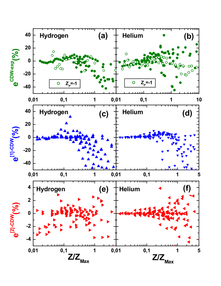
Figure 1: (Color online) Hydrogen target. (a) Relative error of the CDW versus the experiments as defined in Eq.(10) in terms of $Z/Z_{max}$. (c) Relative error of $\sigma^{[1]}$ with respect to the CDW as defined in Eq.(13) (e) Similar to (c) for $\sigma^{[2]}$. (b), (d) and (e) similar to (a), (c) and (f) for helium target.

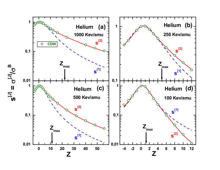
Figure 2: (Color online) Values of $s^{[1]}$ and $s^{[2]}$, as defined in Eq.(11) as a function of the Coulomb incident charge on helium for four impinging energies, as indicated.

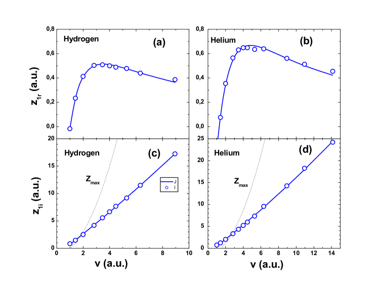
Figure 3: (Color online) Positions of the real and imaginary parts of the pole $Z_{1}$ of $\sigma^{{}^{[}[1]}$, as a function of the impact velocity for hydrogen and Helium as indicated. The symbols are the numerical values and the solid lines are the fitting given by Eqs(12).

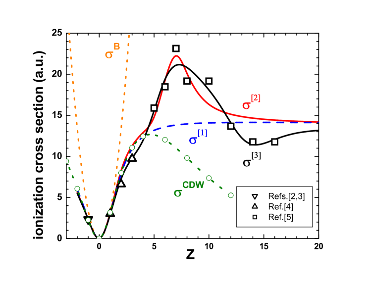
Figure 4: (Color online) Ionization cross section of helium as a function of the incident Coulomb charge for 100kev/amu impact energy. The black empty symbols are the experiments, and first Born approximation, CDW, $\sigma^{[1]}$, $\sigma^{[2]}$, and $\sigma^{[3]}$ as noted.

References

- (1) J. E. Miraglia, ArXiv:2011.08016 [physics.atom-ph]) (2020). Submitted for publication.
- (2) P. Hvelplund, H. U. Mikkelsen, E. Morenzoni, S. P. Moell, E. Uggerhojs and T. Worm, J. Phys. B: At. Mol. Phys. 27, 925–934 (1994)
- (3) L. H. Andersen, P. Hvelplund, H. Knudsen, S. P. Manlier, J. O. P. Pedersen, S. Tang-Petersen, E. Uggerhslj,K. Elsener, and E. Morenzoni, Phys. Rev A 41, 6536–6539 (1990)
- (4) M. B. Shah and H. B. Gilbody, J. Phys. B: At. Mol. Phys. 18, 899–913 (1985)
- (5) S. Datz, R. Hippler, L. H. Andersen, P. F. Dittner, H. Knudsen, H. F. Krause,P. D. Miller, P. L. Pepmiller, T. Rosseel, R. Schuch, N. Stolterfoht, Y. Yamazaki, and C. R. Vane, Phys. Rev A 41, 3559–3571 (1990)
- (6) V. D. Rodriguez, M. S. Gravielle and J. E. Miraglia, Phys. Scripta 43, 52-56 (1991)