Identification of NARX Models for
Compensation Design

Abstract

This report presents the modeling results for three systems, two numerical and one experimental. In the numerical examples, we use mathematical models previously obtained in the literature as the systems to be identified. The first numerical example is a heating system with a polynomial nonlinearity that is described by a Hammerstein model. The second is a Bouc-Wen model that represents the hysteretic behavior in a piezoelectric actuator. Finally, the experimental example is a pneumatic valve that presents a variety of nonlinearities, including hysteresis. For each example, a Nonlinear AutoRegressive model with eXogenous inputs (NARX) is identified using two well-established techniques together, the Error Reduction Ratio (ERR) method to hierarchically select the regressors and the Akaike’s Information Criterion (AIC) to truncate the number of terms. Using both approaches, the structure selection is achieved. The design of the excitation input is based on preserving the frequencies of interest and force the system to achieve different points of operation. Hence, having the structure previously selected with ERR and AIC, we use the Extended Least Squares (ELS) algorithm to estimate the parameters. The results show that it is possible to identify the referred systems with no more than five terms. These identified models will be used for nonlinearity compensation in future works.

I Introduction

For many control applications, the first step is the identification of a representative model to describe the fundamental aspects of the nonlinear dynamical system under investigation. The identification process is usually addressed from a black-box and gray-box perspectives. In the black-box approach, the system is modeled exclusively from data without any prior knowledge of the system. On the other hand, gray-box techniques use the data set and other information about dynamical and static behaviors.

In this sense, it is necessary to define the mathematical representation of the models, such as differential equations [1, 2], Radial Basis Functions (RBFs) [3, 4, 5], Neural Networks (NNs) [6, 7, 8], and Nonlinear AutoRegressive models with eXogenous inputs (NARX) [9, 10], among others. Having the representation selected, the first step is to prepare the data set for identification purposes. In this sense, it is essential to select an adequate sampling time, to excite the system at the frequencies of interest and to achieve different many operation points [11].

Being the data set carefully prepared and an appropriate mathematical framework defined, it is important to select the model structure [12]. The structure selection stage defines which terms from a larger set of candidates will be part of the model. In the sequel, once the structure is known, the model parameters are estimated with some optimization algorithm. The last step is the validation of the model, which includes a different data set than the one used for identification [11].

In this report, we present the modeling results for three systems, being the first two considered as numerical examples, while the last is an experimental. In the numerical examples, we use mathematical models previously obtained in the literature as the systems to be identified. The first numerical example is a heating system with a polynomial nonlinearity that is described by a Hammerstein model. The second is a Bouc-Wen model that describes the hysteretic behavior in a piezoelectric actuator. Finally, the experimental example is a pneumatic valve that presents a variety of nonlinearities, including hysteresis. For each example, a NARX model is identified. The selection of an appropriate structure for the model is done considering the regressors and the number of terms in the model [12]. For this purpose, two well-established techniques are used together, the Error Reduction Ratio (ERR) [13] method and the Akaike’s Information Criterion (AIC) [14]. The ERR aims to sort the most representative regressors in the model, while the AIC truncates the number of terms. A relevant part of this identification process is the design of the excitation input. It is based on preserving the frequencies of interest and force the system to achieve different points of operation. Hence, having the structure previously selected with AIC and ERR, we use the Extended Least Squares (ELS) [15] algorithm to estimate the parameters. The results show that it is possible to identify the referred systems with no more than five terms. In [16], these models will be used for compensation purposes.

II Background

Being a nonlinear dynamical system $\cal S$ with a single input $u(t){\in}\mathbb{R}$, which determines a single output $y_{s}(t){\in}\mathbb{R}$. Consider that a data set with $N{\in}\mathbb{N}^{+}$ samples, $Z^{N}{=}\{{u}(k),{y}_{s}(k)\}^{N}_{k=1}$, was collected from $\cal S$ with a sampling time $T_{\rm s}$. The aim is to identify a Nonlinear Autoregressive model with eXogenous inputs (NARX), namely $\cal M$, for representing the most relevant nonlinear aspects of $\cal S$ [17]:

$$y(k){=}f^{\ell}\big{(}y(k{-}1),\ldots,y(k{-}n_{y}),u(k{-}\tau_{\rm d}),\ldots,u(k{-}n_{u})\big{)},$$ (1)

where $y(k)\in\mathbb{R}$ is the deterministic model output that predicts $y_{s}(k)$, $f^{\ell}(\cdot)$ is a nonlinear polynomial function with degree $\ell\in\mathbb{N}^{+}$. $n_{u},\,n_{y}\in\mathbb{N}^{+}$ are the maximum lags for $u$ and $y$, respectively, $\tau_{\rm d}\in\mathbb{N}^{+}$ is the pure time delay. The $i$-th term $\psi_{i}(k-1)$ of $\cal M$ allows combinations up to degree $\ell$ of the regressor variables $y(k-k_{y})$, for $k_{y}\in\{1,\ldots,n_{y}\}$ and $u(k-k_{u})$, for $k_{u}\in\{\tau_{d},\ldots,n_{u}\}$:

$$\psi_{i}(k-1)=\prod_{k_{y}=1}^{n_{y}}y(k-k_{y})^{\ell_{{y},k_{y}}}\prod_{k_{u}=\tau_{d}}^{n_{y}}u(k-k_{u})^{\ell_{u,k_{u}}},$$ (2)

where

$$\sum_{k_{y}=1}^{n_{y}}\ell_{y,k_{y}}+\sum_{k_{u}=\tau_{d}}^{n_{u}}\ell_{u,k_{u}}=\ell,$$

with $\ell_{y,k_{y}}\in\mathbb{N}$ and $\ell_{u,k_{u}}\in\mathbb{N}$. Model $\cal M$ is composed by $n_{\theta}\in\mathbb{N}^{+}$ terms like (2), each one is multiplied by a constant parameter $\hat{\theta}_{i}$. Thus, $\cal M$ can be expressed as:

$$y(k)=\sum\limits_{i=1}^{n_{\theta}}\hat{\theta}_{i}\psi_{i}(k-1).$$ (3)

Considering the modeling error of $\cal M$ or residues, $\xi(k)=y_{\rm s}(k)-y(k)$, it is possible to rewrite (3) in a convenient form as follows:

$$y_{s}(k)=\bm{\psi}^{T}(k-1)\bm{\hat{\theta}}+\xi(k),$$ (4)

where $\bm{\hat{\theta}}$ is the vector of parameters $[\hat{\theta}_{1},\ldots,\hat{\theta}_{\rm n_{\theta}}]^{T}$, $\bm{\psi}$$(k-1)$ is the set of regressors (2) organized in a vector $[\psi_{1}$$(k-1)$, $\ldots,\psi_{n_{\rm\theta}}(k-1)]^{T}$ and $T$ indicates the transpose. Applying (4), for $k=1,\ldots,N$, over the data set $Z^{N}$, it is possible to build the following equation in matrix form [11]:

$$\bm{y}_{s}=\bm{\Psi}\bm{\hat{\theta}}+\bm{\xi},$$ (5)

where $\bm{\xi}=[\xi(1),\ldots,\xi(N)]^{T}$, $\bm{y}_{s}=[y_{s}(1),\ldots,y_{s}(N)]^{T}$, $\bm{\psi_{i}}=[\psi_{i}(1),\ldots,\psi_{i}(N)]^{T}$ for $i\in\{1,\ldots,n_{\theta}\}$, and $\bm{\Psi}\in\mathbb{R}^{N\times n_{\theta}}$ is the regressor matrix given by $\bm{\Psi}=[\bm{\psi}_{i}(1),\ldots,\bm{\psi}_{i}(N)]^{T}$. As (5) is linear in the parameters, classic regression methods can be used, e.g., Least Squares (LS). The LS method provides the following parameter vector $\bm{\hat{\theta}}_{\rm LS}$ optimal, in the sense of least squares of the modeling error:

$$\bm{\hat{\theta}}_{\rm LS}=[\bm{\Psi}^{T}\bm{\Psi}]^{-1}\bm{\Psi}^{T}\bm{y}_{s}.$$ (6)

When $\xi(k)$ is autocorrelated, the LS method presents a polarized response. This is common in the presence of noise, for which the addition of moving average (MA) terms is an alternative to solve such a problem. However, this addition provides a nonlinear model in the parameters, and the classic LS cannot be used. A way to circumvent this issue is given by the Extended Least Squares (ELS) [12]. This iterative algorithm uses $\xi(k)$ from the previous iteration to extend the regressor matrix, being executed until a convergence criterion is reached, as illustrated by the following steps [15]:

1. Based on Eq. 6, estimate $\bm{\hat{\theta}}_{LS}$;

2. Calculate the vector of residues, $\bm{\xi}_{1}=\bm{y}_{s}-\bm{\Psi\hat{\theta}}_{\rm LS}$;

3. Define the iteration $i=2$ and the convergence limit $\zeta\in\mathbb{R}^{+}$;

4. Build ${\bm{\tilde{\Psi}}_{i}}=[\bm{\Psi}$ ⋮ $\text{ }\bm{\xi}_{i-1}]$, the extended regression matrix;

5. Estimate via LS the new vector of parameters at each iteration: $\bm{\hat{\theta}}_{{\rm ELS}_{i}}=[{\bm{\tilde{\Psi}}_{i}}^{T}\bm{\tilde{\Psi}}_{i}]^{-1}{\bm{\tilde{\Psi}}_{i}}^{T}\bm{y}_{s}$;

6. Determine the current residues: $\bm{\xi}_{i}=\bm{y}_{s}-\bm{\tilde{\Psi}_{i}\hat{\theta}}_{{\rm ELS}_{i}}$;

7. If ${||\bm{\hat{\theta}}_{{\rm ELS}_{i}}-\bm{\hat{\theta}}_{{\rm ELS}_{i-1}}||}_{2}<\zeta$, make $\bm{\hat{\theta}}_{\rm ELS}=\bm{\hat{\theta}}_{{\rm ELS}_{i}}$ and finish the process. Otherwise, make $i=i+1$ and return to step $4$. $||\bullet||_{2}$ is the quadratic norm.

The described technique to determine the parameters must be applied to a previously identified structure. The selection of this structure for $\cal M$ can be done with the following techniques used together.

II-A The Error Reduction Ratio Method

The Error Reduction Ratio (ERR) is an optimization-based technique that quantifies the contribution of each term to explain the variance of the modeling error [13]. For this application, each model regressor must be orthogonal to the data that can be achieved with Householder transformation [18]. Taking the average value of $y_{s}(k)^{2}$ on the data, it is possible to find the following expression [12]:

$$\dfrac{1}{N}\sum\limits_{k=1}^{N}y_{s}(k)^{2}=\sum\limits_{i=1}^{n_{\theta}}{\hat{\theta}_{i}}^{2}{\bm{{w_{i}}^{T}}}{\bm{w_{i}}}+{\bm{\xi^{T}}}{\bm{\xi}}.$$ (7)

The error reduction ratio due to the inclusion of $i$-th regressor is given by the following expression:

$$|ERR_{i}|=\dfrac{{\hat{\theta}_{i}}^{2}{\bm{{w_{i}}^{T}}}{\bm{{w_{i}}}}}{\bm{y^{T}y}}.$$ (8)

The inclusion of each term in the model reduces the variance of the modeling error. The index $|ERR_{i}|$ quantifies the contribution of the $i$-th term in the reduction of this variance. By selecting the regressors that provide the highest values for this index, it is possible to reduce the candidate set. This is relevant because the number of regressor candidates tends to considerably increase with the raise of $\ell$ [12]. However, this technique only sorts the candidate terms hierarchically, it is still necessary to choose the number of candidate terms.

II-B The Akaike’s Information Criterion

The Akaike’s Information Criterion (AIC) is a tool that helps to define the number of terms to be included in the model, based on minimizing a cost function [14]. The addition of new terms increases the model complexity, which allows a better fit. Considering that the terms were sorted with ERR, a given number of terms $n_{\theta}$ is enough to determine ${\cal M}_{n_{\theta}}$ with an output $y_{n_{\theta}}(k)$. The polarized error is the variance of the residues of this model, $\sigma_{\xi}^{2}(n_{\theta})=\sigma^{2}[y_{s}(k)-y_{n_{\theta}}(k)]$. When $n_{\theta}$ increases, $\sigma_{\xi}^{2}(n_{\theta})$ tends to reduce, although increases in complexity do not guarantee a better generalization performance. Thus, this criterion aims to penalize the rise in the number of terms. The AIC cost function is:

$$J_{AIC(n_{\theta})}=N{\rm ln}[\sigma_{erro}^{2}(n_{\theta})]+2n_{\theta}.$$ (9)

Hence, this function tends to achieve a minimum value for some value of $n_{\theta}$. It is convenient to highlight that this is a purely statistical criterion that helps in the identification process. Thus, there is no guarantee that the obtained model is valid in the identification perspective.

II-C NARX Hysteresis Modeling

Sufficient conditions for NARX models to mimic hysteresis loops were presented by [19]. The authors have shown that with the inclusion of the first difference of the input $\phi_{1}(k){=}u(k){-}u(k{-}1)$ and its corresponding sign function, $\phi_{2}(k){=}{\rm sign}(\phi_{1}(k))$, it is possible to represent a hysteretic behavior for loading-unloading inputs. A general extended deterministic NARX model set [20] referred as ${\cal{M}}_{\rm h}$ is represented by:

$$\!\!\!\!\!y(k) {=} g^{\ell}\big{(}y({k-1}),\cdots,y(k-n_{y}),\,u(k-\tau_{\rm d}),\cdots,$$ (10)

$$\hskip 8.53581ptu(k-n_{u}),\phi_{1}(k-1),\,\phi_{2}(k-1)\big{)},$$

where $g^{\ell}(\cdot)$ is a polynomial function of the regressor variables up to degree $\ell$, and the other parameters are previously mentioned. Model ${\cal M}_{\rm h}$ (10) presents two sets of equilibria under loading-unloading inputs: one for loading with $\phi_{2}(k){=}1$, and one for unloading with $\phi_{2}(k){=}{-}1$ [19, 9].

It has been shown that for ${\cal{M}}_{\rm h}$, some regressors can be excluded, regardless of the lags $\tau_{u}$ and $\tau_{y}$ [9], as summarized below:

• $y^{p}(k-\tau_{y})$, $y^{p}(k-\tau_{y})\phi_{1}(k-\tau_{u})^{q}$,
  $y^{p}(k-\tau_{y})\phi_{2}(k-\tau_{u})^{q}$ for $p{>}1,~{}\forall q$, [21],

• $\phi_{2}^{q}(k-\tau_{u})$ for $q>1$ [19], and

• $y^{p}(k-\tau_{y})u^{m}(k-\tau_{u})$ and $u^{m}(k-\tau_{u})$, $\forall p,m$ [9].

It is important to note that such constraints are specified for the identification of ${\cal{M}}_{\rm h}$, as detailed in the references. Considering $\Sigma_{y}$, as the sum of parameters of all linear output regressors, if a model is identified with these constraints and forcing the parameters to generate $\Sigma_{y}=1$, the model remains in the last state when the reference becomes constant. This property is desired for hysteresis models and can be achieved using a constrained least squares estimator, as detailed in [9].

III The Identification Methodology

The procedure proposed here takes into account the need to excite the system in a wide frequency range and reach a variety of operating points [22]. Therefore, the procedure starts with the need to define the frequencies, $f_{i}\in\mathbb{R}^{+}$ for $i{=}1,\ldots,n$, that will be preserved in the signal. For instance, in the case of hysteretic systems, it is necessary to preserve low-frequency information in the identification data [23]. To circumvent this type of problem, the fifth-order low-pass Butterworth filters, ${\cal H}_{i}(q)$, are designed with a cutoff frequency that concentrates the spectral power of interest. In this work, we consider that these filters are applied to a purely random signal $e_{i}(k){=}{\cal N}(0,\,1),~{}k=1,\,2,\ldots N_{i}$ where ${\cal N}(0,\,1)$ is a standard normal distribution. Each signal $e_{i}(k)$ is conditioned to have $1$ as maximum and $-1$ as minimum, given by:

$$e_{i}(k)=2\left(\dfrac{e_{i}(k)-{\rm min}[e_{i}(k)]}{{\rm max}[e_{i}(k)]-{\rm min}[e_{i}(k)]}\right)-1,$$ (11)

and its number of samples $N_{i}$ is specified to have an input signal $u(k)$ with $N$ samples, such that $N{=}N_{1}{+}N_{2}{+}\cdots{+}N_{n}$. As will be seen, the input signal $u(k)$ is obtained by concatenating a signal $s_{i}(k)$, for $i{=}1,\ldots,n$.

To ensure that the signal $u(k)$ can achieve a variety of operating regions, it is considered the operations points as $o_{j}\in\mathbb{R}$ for $j{=}1,\ldots,v$. For each operation point $o_{j}$, it is defined an amplitude $G_{j}$ around this particular point. In addition, the values assigned for each number of samples $N_{i}$ must be defined as multiples of the number of operating points, $v$. This is necessary since it is intended that each frequency has information around all operating points. In this way, the signal $s_{i}(k)$ that is a part of $u(k)$ can be produced as follows:

$$s_{i}(k){=}\left\{\begin{array}[]{ll}\!\alpha_{i,1}{\cal H}_{i}(q)e_{i}(k)+o_{1},&k{=}1,\,2,\ldots\dfrac{N_{i}}{v}\\ \!\vdots&\vdots\\ \!\alpha_{i,v}{\cal H}_{i}(q)e_{i}(k)+o_{v},&k=(v{-}1)\dfrac{N_{i}}{v}{+}1,\\ &\hskip 11.38109pt(v{-}1)\dfrac{N_{i}}{v}{+}2,\ldots,N_{i}.\\ \end{array}\right.$$ (16)

The constants $\alpha_{i,j}$ are defined to limit the excursion of the input around each operating point. For a given operating point $o_{j}$, we have $\alpha_{i,j}{=}G_{j}/{\rm{max}}[e_{i}(k_{i,j})]$ for which $k_{i,j}=(j-1)(N_{i}/v)+1,(j-1)(N_{i}/v)+2,\ldots,j(N_{i}/v)$. Applying (16) for $i=1,2,\ldots,n$, we get $s_{1},s_{2},\ldots,s_{n}$ and the $u(k)$ is the concatenation of these inputs:

$$u(k)=[s_{1}\quad s_{2}\quad\ldots\quad s_{n}].$$ (17)

Finally, selecting the maximum frequency $f_{i}$, the low-pass filter related to this frequency is used to eliminate possible higher frequencies originating from concatenation.

This procedure is performed twice, in order to have different realizations for identification and validation inputs, which are applied to the system for data collection. To achieve more robust experiments, Gaussian noise was added directly to the output to obtain $\sigma_{n}/\sigma_{s}=5\%$, where $\sigma_{n}$ is the standard deviation of the noise, and $\sigma_{s}$ is the standard deviation of the signal. To complement our validation data, we also generate sinusoidal inputs at different frequencies and amplitudes.

Considering the model structure selection step, the ERR and AIC tools are used together, as detailed in Sec. II. First, the candidate regressors to compose the NARX model are evaluated and ranked in such way that the ERR criterion is minimized. Then, the AIC is used to truncate the number of regressors in the final model. For the estimation of parameters, in this paper, the ELS method is used.

IV Examples

This section illustrates the identification procedure proposed in Sec. III for two simulated benchmark systems and one experimental. The first one is a heating system modeled by a Hammerstein model with a polynomial nonlinearity, and the second is a Bouc-Wen that aims to model the hysteresis of a piezoelectric (PZT) device. The experimental example is a pneumatic valve. All examples are treated as systems to be modeled and these models are used for compensation in [16]. To evaluate the performance of the prediction and compensation achieved, the mean absolute percentage error (MAPE) index is computed as follows:

$${\rm{MAPE}}=\dfrac{\sum_{k=1}^{N}|y(k)-\hat{y}(k)|}{N|{\max}({\bm{y}})-{\min}({\bm{y}})|}.$$ (18)

IV-A A Heating System

Consider the bench test system, a small electrical heater, modeled by the following Hammerstein model [24]:

$$y(k)= \beta_{1}y(k-1)+\beta_{2}v(k-1)+\beta_{3}y(k-2)+\beta_{4}v(k-2),$$

$$v(k)= p_{1}u(k)^{2}+p_{2}u(k),$$ (19)

where $y(k)$ is the normalized temperature, and $u(k)$ is the electric power applied to the heater within the range $0{\leq}u(k){\leq}1$. The data set of such a system is the same considered in [25], which is available at https://bit.ly/3iQ6rCF. Here, we reestimate the parameters of model (IV-A), obtaining: $p_{1}=4.639331\times 10^{-1}$, $p_{2}=5.435865\times 10^{-2}$, $\beta_{1}=1.205445$, $\beta_{2}=8.985133\times 10^{-2}$, $\beta_{3}=-3.0877507\times 10^{-1}$ and $\beta_{4}=9.462358\times 10^{-3}$. This reestimation was need because the parameters provided by [24] have few decimal digits, which severely impact in the results for discrete systems.

The independent term in the second-order polynomial that gives $v(k)$ was omitted in order to ensure $y=0$ when $u=0$. $p_{1}$ and $p_{2}$ were estimated directly from static data using LS, although $\beta$’s were estimated from dynamical data using ELS algorithm. The operation region of the model is $u(k)\in[0,~{}1]$ and $y(k)\in[0,~{}0.5]$. The validation result (Fig. 1) shows the performance of the model given by (IV-A).

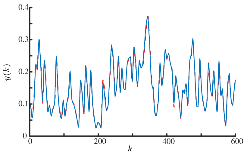
Figure 1: Performance of (IV-A) over measured validation data provided by [25]. Continuous line (–) is the measured data, while the dashed line (- -) is the free-run simulation of model (IV-A).

From now on, the Hammerstein model (IV-A) will be treated as the system $\cal{S}$ to be identified with a NARX polynomial model $\cal{M}$ (1). The input $u(k)$ was designed following (16) and (17) with: $n=2$, $f_{1}=0.001{\rm{Hz}}$, $f_{2}=0.005{\rm{Hz}}$, $v=3$, $o_{1}=0.3{\rm{V}}$, $o_{2}=0.5{\rm{V}}$, $o_{3}=0.7{\rm{V}}$, $G_{1}=G_{2}=G_{3}=0.2{\rm V}$, $N=2000$, $N_{1}=1000$, and $N_{2}=1000$. Figure 2 shows the results obtained with Monte Carlo Tests to assess how the predictive capacity of the identified models degrade with the increase the noise power, using the MAPE index. Considering the system output $y_{s}(k)$, for each Monte Carlo test, a Gaussian noise is added with a given value of the ratio $\sigma_{n}/\sigma_{s}$, where $\sigma_{n}$ is the standard deviation of the noise, and $\sigma_{s}$ is the standard deviation of the signal. The $\sigma_{n}/\sigma_{s}$ values vary from $0\%$ to $30\%$ with successive increase of $2\%$. For each $\sigma_{n}/\sigma_{s}$ value, $50$ perturbed output signals are generated and their respective models are identified taking into account the previous recommendations. Finally, we get the mean and standard deviation of MAPE for each $\sigma_{n}/\sigma_{s}$ value. From Fig. 2 is possible to see that the model quality of the identification is, in average, more frequently affected for raising values of $\sigma_{n}/\sigma_{s}$. Also, the predictability is harmed, since there is an enlargement in the confidence intervals.

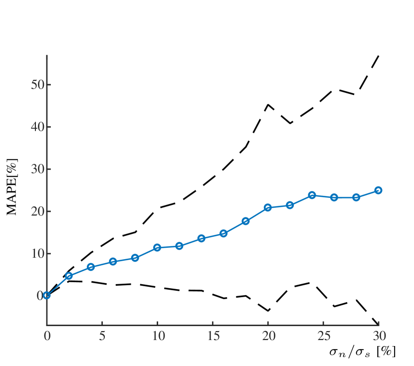
Figure 2: Monte Carlo tests are performed to evaluate the MAPE [%] variation in function of the raising from $\sigma_{n}/\sigma_{s}$ [%] where $\sigma_{n}$ is the standard deviation of the noise, and $\sigma_{s}$ is the standard deviation of the signal. For each $\sigma_{n}/\sigma_{s}$ value, 50 Monte Carlo tests are performed. We show the mean of 50 tests ($\ominus$) and $\pm$2 standard deviations (- -). The continues lines (–) are only illustrative, since the tests were taken for successive raises of 2% in $\sigma_{n}/\sigma_{s}$.

As aforementioned, in the examples used, Gaussian noise was added directly to the output to yield a $\sigma_{n}/\sigma_{s}=5\%$. Taking $\ell=3$ and $n_{y}=n_{u}=3$, the ERR method selects the more representative regressors and the AIC criterion is calculated as shown in Fig. 3.

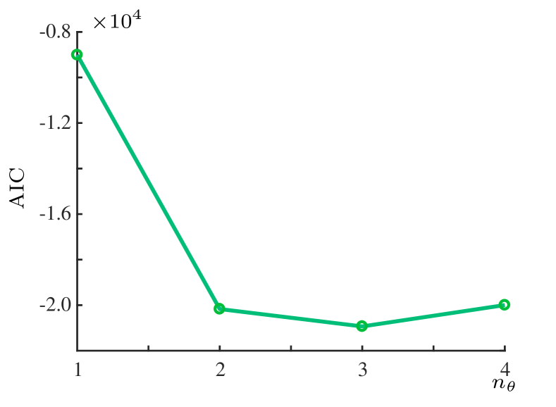
Figure 3: AIC criterion used for the definition of $n_{\theta}$. It has been chosen the model of 3 terms due to the index minimization. The continuos line have no meaning, it was used for facilitates the visualization.

By minimizing the AIC criterion, the following three-term model $\cal M$ was obtained according to the procedure detailed in Sec III:

$$y(k)=\hat{\theta}_{1}y(k-1)+\hat{\theta}_{2}u(k-2)^{2}+\hat{\theta}_{3}y(k-2),$$ (20)

where $\hat{\theta}_{1}=8.958185\times 10^{-1}$, $\hat{\theta}_{2}=6.393347\times 10^{-2}$, and $\hat{\theta}_{3}=-1.746750\times 10^{-2}$. The free-noise results for the validation data set are shown in Fig. 4. A more detailed assessment of this model for sinusoidal inputs can be found in Table I in [16]. The mentioned work provide an compensation approach based on this identified model.

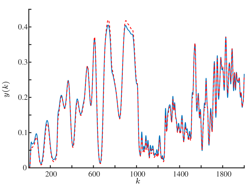
Figure 4: Noise-free validation data for model $\cal M$ (20): continuous line (–) presents values of $y(k)$ for the system $\cal S$ (IV-A), while the dashed line (- -) is the free-run simulation of model (20).

IV-B A Hysteretic System

In this example, the following Bouc-Wen model was used to describe the hysteretic behavior of a piezoelectric actuator (PZT) that is an unimorph cantilever [26]:

$$\dot{h}(t)= \alpha_{\rm bw}\dot{u}(t)-\beta_{\rm bw}|\dot{u}(t)|h(t)-\gamma_{\rm bw}\dot{u}(t)|h(t)|,$$

$$y(t)= \nu_{y}u(t)-h(t),$$ (21)

where $u(t)$[V] is the voltage input, $y(t)$[$\rm{\mu}m$] is the position output, the parameters $\alpha_{\rm bw}=0.9[\mu\rm{m}/\rm{V}]$ and $\beta_{\rm bw}=\gamma_{\rm bw}=0.008[\rm{V}^{-1}]$ determine the hysteresis loop, while $\nu_{y}=1.6[\mu\rm{m}/\rm{V}]$ is a weight factor for the output. Here, (21) is referred as the system $\cal S$ to be identified, which is simulated with a fourth-order Runge-Kutta method considering the integration step $\delta_{t}=5\rm{ms}$.

To identify a NARX polynomial model ${\cal M}_{\rm h}$ (10) for $\cal S$, the identification input $u(k)$ is designed according to (16) and (17) with: $n=2$, $f_{1}=0.2{\rm{Hz}}$, $f_{2}=5{\rm{Hz}}$, $v=2$, $o_{1}=o_{2}=0{\rm{V}}$, $G_{1}=25{\rm V}$, $G_{2}=50{\rm V}$, $N=19200$, $N_{1}=16000$ and $N_{2}=3200$. Gaussian noise was added directly to the output to yield a $\sigma_{n}/\sigma_{s}=5\%$, as in the previous example. At higher noise levels the identified models are somewhat worse, as expected, similarly the discussion previous done in Sec.IV-A. Based on Sec. II-C, $u(k)$, $y(k)$, $\phi_{1}(k){=}u(k){-}u(k{-}1)$, and $\phi_{2}(k){=}{\rm sign}(\phi_{1}(k))$ are chosen as candidate regressors, taking $\ell=3$ and $n_{y}=n_{u}=1$ the following forth-term model ${\cal M}_{\rm h}$ was obtained from AIC and ERR to select the structure, and ELS for parameter estimation:

$$y(k)\!\!\!\! {=} \!\!\!\!\hat{\theta}_{1}y(k{-}1){+}\hat{\theta}_{2}\phi_{2}(k{-}1)\phi_{3}(k{-}1)u(k{-}1)$$ (22)

$${+}\hat{\theta}_{3}\phi_{2}(k{-}1)\phi_{3}(k{-}1)y(k{-}1){+}\hat{\theta}_{4}\phi_{2}(k{-}1),$$

where $\hat{\theta}_{1}=1.000099$, $\hat{\theta}_{2}=6.630567\times 10^{-3}$, $\hat{\theta}_{3}=-6.247018\times 10^{-3}$, and $\hat{\theta}_{4}=7.892915$. Note that this model has a structure which consent with the restrictions (i), (ii), and (iii) of Sec. II-C. However, this model does not comply with the constrained $\Sigma_{y}=1$. The validation results are shown in Fig. 5, and in Table III that is shown in [16]. Figure 5 shows a free-noise simulation with the output prediction showed for two parts: (a) excited for $f_{1}=0.2$ with $0\leq k\leq 16000$; and (b) for $f_{2}=5$ with $16000\leq k\leq 18000$.

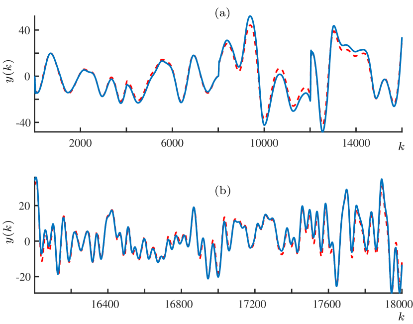
Figure 5: Noise-free validation data for model ${\cal M}_{\rm h}$ (22): continuous line (–) presents values of $y(k)$ for the system $\cal S$ (21); dashed line (- -) presents output values of the model (22). In (a), we have the temporal evolution of the outputs for lower frequency $f_{1}=0.2\rm{Hz}$ $(0\leq k\leq 16000)$, while in (b) is shown the first 3000 samples for higher frenquency $f_{2}=5\rm{Hz}$, $(16001\leq k\leq 18000)$.

IV-C Experimental Results

This section consider the identification process for a pneumatic valve. The NARX model obtained provides results that are compared with models proposed by [26] and [9]. See [16] for more details. The present pneumatic valve is the same used in [9], where the measured output is its stem position and the input is a pressure signal applied to the valve after passing V/I and I/P conversion. The sampling time is $T_{\rm s}=0.01\,{\rm s}$ and, for model identification, the same input designed in [9] is used, which is set as white noise low-pass filtered at $0.1\,{\rm Hz}$ similarly to what is done in the sections above, but for only one frequency. For model validation, the inputs are sine waves with frequency $0.1\,{\rm Hz}$ and different amplitudes. All these data sets are $200\,{\rm s}$ long ($N=20000$).

The first NARX model below is obtained for this system using the identification strategy based on the ERR and AIC criterion, as explained in Sec. III and previous examples. The candidate terms to compose these models are generated with $\ell=3$, $n_{y}=2$ and $n_{u}=1$.

1) ${\cal M}_{\rm h}$ describes the model identified with the inclusion of $\phi_{1}(k)$ and $\phi_{2}(k)$, and also adopts the constraints proposed by [9]. These constraints are: the exclusion of some regressors showed in (i), (ii) and (iii), and force the parameters to comply with $\Sigma_{y}=1$, see Sec. II-C. The identified model is:

$$y(k) = \hat{\rho}_{1}y(k-1)+\hat{\rho}_{2}y(k-2)+\hat{\rho}_{3}\phi_{1}(k-1)$$ (23)

$$+ {\rho}_{4}u(k-1)\phi_{1}(k-1)\phi_{2}(k-1)$$

$$+ \hat{\rho}_{5}y(k-2)\phi_{1}(k-1)\phi_{2}(k-1),$$

with $\hat{\rho}_{1}=9.76\times 10^{-1}$, $\hat{\rho}_{2}=2.40\times 10^{-2}$, $\hat{\rho}_{3}=1.19\times 10^{-1}$, $\hat{\rho}_{4}=3.76$ and $\hat{\rho}_{5}=-4.73$. Note that, $\Sigma_{y}=\hat{\rho}_{1}+\hat{\rho}_{2}=1$.

In what follows, three models already established in the literature are considered for comparison purposes. The first one is a hysteresis model based on a phenomenological approach, which is stated below.

2) ${\cal M}_{\rm bw}$ is used to represent a Bouc-Wen model previously shown in (21). To estimate the valve output, its parameters were re-estimated using an evolutionary approach based on niches, which is formulated in [27]. The obtained model is:

$$\dot{h}(t)= 7.54\times 10^{-1}\dot{u}(t)-4.96|\dot{u}(t)|h(t)-3.61\dot{u}(t)|h(t)|,$$

$$y(t)= 7.21\times 10^{-1}u(t)-h(t).$$ (24)

The last two models adopted were identified in [9] for the same system under study and with the same identification data. However, the meta-parameters of the identification process were $\ell=3$, $n_{y}=2$ and $n_{u}=2$.

3) ${\cal M}_{\rm h,2}$ symbolizes the model identified with the same constraints used for ${\cal M}_{\rm h}$ (23), plus an additional one required by the compensation strategy so that the input signal can be isolated, see [9]. The estimated model in the mentioned paper was:

$$y(k) =y(k-1)-19.76\phi_{1}(k-2)+19.32\phi_{1}(k-1)$$

$${+}9.44\phi_{2}(k-2)\phi_{1}(k-2)u(k{-}2)$$

$${-}12.61\phi_{2}({k{-}2})\phi_{1}(k{-}2)y(k{-}1).$$ (25)

4) ${\breve{\cal M}}_{\rm h}$ represents the model identified to describe the inverse relationship between $u(k)$ and $y(k)$ of the valve. Therefore, the model output is the estimated input $\hat{u}(k)$, the system output $y(k)$ becomes the model input, and the candidate regressors $\breve{\phi}_{1}(k)=y(k)-y(k-1)$ and $\breve{\phi}_{2}(k)={\rm sign}[\breve{\phi}_{1}(k)]$ are included. Following the same constraints used for ${\cal M}_{\rm h,cns}$ (23) with appropriate conversions for the inverse model, [9] have got the following model:

$$\hat{u}(k) =\hat{u}({k{-}1})+86.67\breve{\phi}_{1}(k{-}1)-85.02\breve{\phi}_{1}(k{-}2)$$

$${-}0.98\breve{\phi}_{1}(k{-}1)y({k{-}2})+1.72\breve{\phi}_{2}(k{-}2)\breve{\phi}_{1}(k{-}2)y(k{-}2)$$

$${-}1.13\breve{\phi}_{2}(k{-}2)\breve{\phi}_{1}(k{-}2)\hat{u}(k{-}1).$$ (26)

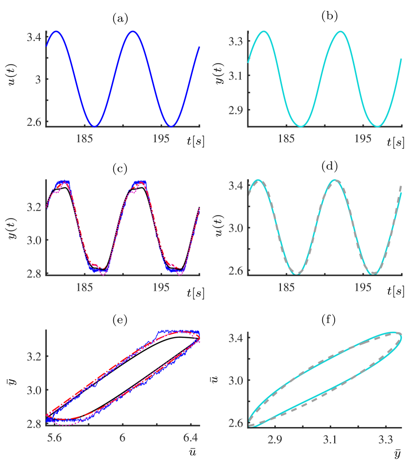
Figure 6: Free-run validation of the presented models obtained for the pneumatic valve. (a), (b) and (c) refer to the direct models which predict the output $y(t)$. In (c), the outputs $y(t)$ are shown for the models excited by the input (a), $u(t)=0.45{\rm sin}(2\pi(0.1)t+\pi/4)+3$V. (e) is the plane $\bar{u}\times\bar{y}$ which shows the hysteretic loop. (b), (d) and (f) are the analogous respectively for (a), (c) and (e), but to the inverse model ${\breve{\cal M}}_{\rm h}$ (IV-C) (- -) since it predicts the input $u(t)$ based on an smooth version of $y(t)$ showed in (b). (–), refers to the system in the direct context while (–), to the inverse. (-$\dotproduct$-), ${\cal M}_{\rm h}$ (23); (–), ${\cal M}_{\rm bw}$ (24); ($\dotproduct$ $\dotproduct$) ${\cal M}_{\rm h,2}$, (IV-C).

The performance of each model is presented in Fig. 6, considering a free-run simulation for $u(t)=0.55{\rm sin}(2\pi(0.1)t+\pi/4)+3$V that is showed in Fig. 6-(a). In Fig. 6-(b), the temporal evolution of the models’ outputs are illustrated, while Fig. 6-(c) presents the hysteretic curve in the plane $\bar{u}\times\bar{y}$. For a different perspective, the inverse model ${\breve{\cal M}}_{\rm h}$ is feed by a smooth version of the system output - Fig. 6-(b) - to predict the corresponding input in the Fig. 6-(d). The MAPE accuracy achieved for this figure is $1.8\%$ and the plane $\bar{y}\times\bar{u}$ is shown in Fig. 6-(f). Other MAPE results are provided in Table V in [16].

V Conclusion

This work has presented three identified models for two numerical examples, and one experimental. An appropriate design of the excitation signal is provided since we select the frequencies that will be preserved and the operation regions to be achieved. The obtained models are simple, having no more than 5 terms. A natural step is use these models in the nonlinearity compensation context, which will be studied in [16].

References

- [1] C. Lin, H. Yau, and Y. Tian, “Identification and Compensation of Nonlinear Friction Characteristics and Precision Control for a Linear Motor Stage,” IEEE/ASME Transactions on Mechatronics, vol. 18, no. 4, pp. 1385–1396, 2013.
- [2] L. Liu, L. Li, Y. Huang, K. Cui, Q. Xiong, F. N. Hauske, C. Xie, and Y. Cai, “Intrachannel nonlinearity compensation by inverse volterra series transfer function,” Journal of Lightwave Technology, vol. 30, no. 3, pp. 310–316, 2011.
- [3] H. Cao, Y. Zhang, C. Shen, Y. Liu, and X. Wang, “Temperature energy influence compensation for MEMS vibration gyroscope based on RBF NN-GA-KF method,” Shock and Vibration, vol. 2018, 2018.
- [4] Y. Zhou, A. Wang, P. Zhou, H. Wang, and T. Chai, “Dynamic performance enhancement for nonlinear stochastic systems using RBF driven nonlinear compensation with extended Kalman filter,” Automatica, vol. 112, p. 108693, 2020.
- [5] J. Li and H. Tian, “Position control of SMA actuator based on inverse empirical model and SMC-RBF compensation,” Mechanical Systems and Signal Processing, vol. 108, pp. 203–215, 2018.
- [6] X. Zhang, Y. Tan, M. Su, and Y. Xie, “Neural networks based identification and compensation of rate-dependent hysteresis in piezoelectric actuators,” Physica B: Condensed Matter, vol. 405, no. 12, pp. 2687–2693, 2010.
- [7] K. Guo, Y. Pan, and H. Yu, “Composite learning robot control with friction compensation: a neural network-based approach,” IEEE Transactions on Industrial Electronics, vol. 66, no. 10, pp. 7841–7851, 2018.
- [8] D. Meng, P. Xia, K. Lang, E. C. Smith, and C. D. Rahn, “Neural network based hysteresis compensation of piezoelectric stack actuator driven active control of helicopter vibration,” Sensors and Actuators A: Physical, vol. 302, p. 111809, 2020.
- [9] P. E. O. G. B. Abreu, L. A. Tavares, B. O. S. Teixeira, and L. A. Aguirre, “Identification and nonlinearity compensation of hysteresis using NARX models,” Nonlinear Dynamics, vol. 102, no. 1, pp. 285–301, 2020.
- [10] W. Lacerda Junior, S. A. M. Martins, E. Nepomuceno, and M. Lacerda, “Control of Hysteretic Systems Through an Analytical Inverse Compensation based on a NARX model,” IEEE Access, vol. PP, pp. 1–1, 07 2019.
- [11] L. A. Aguirre, “A Bird‘s Eye View of Nonlinear System Identification,” arXiv:1907.06803 [eess.SY], 2019.
- [12] S. A. Billings, Nonlinear system identification: NARMAX methods in the time, frequency, and spatio-temporal domains. John Wiley & Sons, 2013.
- [13] M. Korenberg et al., “Orthogonal parameter estimation algorithm for non-linear stochastic systems,” Journal of Control, vol. 48, pp. 193–210, 1987.
- [14] H. Akaike, “A New Look at the Statistical Model Identification,” IEEE Transactions on Automatic Control, vol. 19, no. 6, pp. 716–723, 1974.
- [15] L. Ljung et al., “Theory for the user,” in System Identification. Prentice-hall, Inc., 1987.
- [16] L. A. Tavares, P. E. O. G. B. Abreu, and L. A. Aguirre, “Nonlinearity Compensation Based on Identified NARX Polynomials Models,” Submitted, 2020.
- [17] I. J. Leontaritis and S. A. Billings, “Input-output parametric models for nonlinear systems part I: Deterministic nonlinear systems,” vol. 41, no. 2, pp. 303–328, 1985.
- [18] A. S. Householder, “Unitary triangularization of a nonsymmetric matrix,” Journal of the ACM (JACM), vol. 5, no. 4, pp. 339–342, 1958.
- [19] S. A. M. Martins and L. A. Aguirre, “Sufficient Conditions for Rate-Independent Hysteresis in Autoregressive Identified Models,” Mechanical Systems and Signal Processing, vol. 75, pp. 607–617, 2016.
- [20] S. A. Billings and S. Chen, “Extended model set, global data and threshold model identification of severely nonlinear systems,” vol. 50, no. 5, pp. 1897–1923, 1989.
- [21] L. A. Aguirre and E. M. A. M. Mendes, “Global Nonlinear Polynomial Models: Structure, Term Clusters and Fixed Points,” International Journal of Bifurcation and Chaos, vol. 6, no. 2, pp. 279–294, 1996.
- [22] J. Schoukens and L. Ljung, “Nonlinear system identification: A user-oriented road map,” IEEE Control Systems Magazine, vol. 39, no. 6, pp. 28–99, 2019.
- [23] F. Ikhouane and J. Rodellar, Systems with Hysteresis: Analysis, Identification and Control Using the Bouc-Wen Model. John Wiley & Sons, 2007.
- [24] L. A. Aguirre, M. C. S. Coelho, and M. V. Corrêa, “On the interpretation and practice of dynamical differences between Hammerstein and Wiener models,” Proc. IEE Part D: Control Theory and Applications, vol. 152, no. 4, pp. 349–356, 2005.
- [25] L. A. Aguirre, M. Corrêa, and C. C. S. Cassini, “Nonlinearities in NARX polynomial models: representation and estimation,” Proc. IEE Part D: Control Theory and Applications, vol. 149, no. 4, pp. 343–348, 2002.
- [26] M. Rakotondrabe, “Bouc-Wen Modeling and Inverse Multiplicative Structure to Compensate Hysteresis Nonlinearity in Piezoelectric Actuators,” IEEE Transactions on Automation Science and Engineering, vol. 8, no. 2, pp. 428–431, 2011.
- [27] L. A. Tavares, P. E. O. G. B. Abreu, and L. A. Aguirre, “Estimação de Parâmetros de Modelos Bouc-Wen via Algoritmos Evolutivos para Compensação de Histerese,” in Anais do 14º Simpósio Brasileiro de Automação Inteligente, 2019.