Classification by Attention:
Scene Graph Classification with Prior Knowledge

Abstract

A major challenge in scene graph classification is that the appearance of objects and relations can be significantly different from one image to another. Previous works have addressed this by relational reasoning over all objects in an image or incorporating prior knowledge into classification. Unlike previous works, we do not consider separate models for perception and prior knowledge. Instead, we take a multi-task learning approach, where we implement the classification as an attention layer. This allows for the prior knowledge to emerge and propagate within the perception model. By enforcing the model also to represent the prior, we achieve a strong inductive bias. We show that our model can accurately generate commonsense knowledge and that the iterative injection of this knowledge to scene representations leads to significantly higher classification performance. Additionally, our model can be fine-tuned on external knowledge given as triples. When combined with self-supervised learning and with 1% of annotated images only, this gives more than 3% improvement in object classification, 26% in scene graph classification, and 36% in predicate prediction accuracy.

Introduction

Classifying objects and their relations in images, also known as scene graph classification, is a fundamental task in scene understanding and can play an essential role in applications such as recommender systems, visual question answering and decision making. Scene graph (SG) classification methods typically have a perception model that takes an image as input and generates a graph that describes the given image as a collection of (head, predicate, tail). One of the main challenges that current models face is diverse appearances of objects and relations across different images. This can be due to variations in lighting conditions, viewpoints, object poses, occlusions, etc. For example, the Bowl in Figure 1 is highly occluded and has very few image-based features. Therefore, a typical perception model fails to classify it. One approach to tackle this problem is to collect supportive evidence from neighbors before classifying an entity. This can be done, for example, by message passing between all the image-based object representations in an image, using graph convolutional neural networks (GCN) (Kipf and Welling 2016) or LSTMs (Hochreiter and Schmidhuber 1997). The main issue with this approach is the combinatorial explosion of all possible image-based neighbor representations.

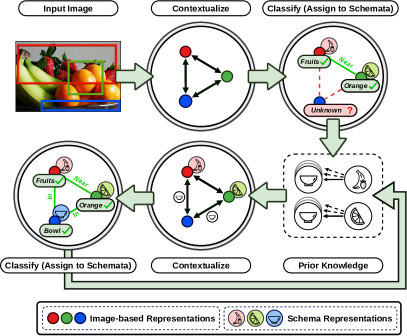
Figure 1: An example of scene graph classification where the Bowl lacks sufficient visual input. Top right is the initially predicted graph from visual inputs only. Bottom left is the prediction of our model after considering both image-based representations and schematic prior knowledge about Fruits and Oranges. The long arrow near the bottom indicates recursion.

A current theory in cognitive psychology states that humans solve this challenge by reasoning over the pre-existing representations of neighboring objects instead of relying on the perceptual inputs only (Piaget 1923); philosophers often argue that humans have a form of mental representation for objects and concepts (Kant 1787). These representations do not depend on a given image but are rather symbol-based. There are different opinions on how these representations come to be. Piaget called these representations schema (plural schemata) and suggested that we acquire them in our earlier perceptions. When an object is being perceived, the mind assigns it to a schema in a process called assimilation. By relational reasoning over schemata, assimilation helps to predict the facts surrounding the observation (Arbib 1992).

Nevertheless, learning and utilizing prior knowledge is still a significant challenge in AI research. Recently,  Zellers et al. (2018) and Chen et al. (2019c, b) proposed to correct the SG prediction errors by comparing them to the co-occurrence statistics of triples in the training dataset or an external source. The statistics can, for example, suggest that it is common to see (Fruits, in, Bowls). Furthermore, instead of relying on simple co-occurrence statistics, one can create a prior model with knowledge graph embeddings (KGE) (Nickel et al. 2016) that can generalize beyond the given triples (Baier, Ma, and Tresp 2017, 2018; Hou et al. 2019). KGEs typically consist of an embedding matrix, that assigns a vector representation to each entity, and an interaction function that predicts the probability of a triple given the embeddings of its head, predicate, and tail. This allows KGE models to generalize to unseen relations. For example, Man and Woman will be given similar embeddings since they appear in similar relations during the training. As a result, if the model observes (Woman, rides, Horse), it can generalize, for example, to (Man, rides, Camel).

However, in the described approaches, unlike Piaget’s schemata, the perception and the prior are treated naively as independent components; they are trained separately and from different inputs (either from images or from triples), and their predictions are typically fused in the probability space, e.g., by multiplication. Other than requiring redundant parameters and computations, this makes the prior model agnostic to the image-based knowledge and the perception model agnostic to the prior knowledge. For example, the collection of triples might contain (Woman, rides, Horse) but have no triples regarding a Donkey. While the images can represent the visual similarities of a Horse to a Donkey, the triples lack this information. If we train a prior model purely based on the triples, the model fails to generalize. We can avoid this by training the prior model from a combination of triples and images. As for another example, in Figure 1, the prior model might suggest (Fruits, in, Bowl) but it might also suggest (Fruits, areOn, Trees). To decide between the two, one should still consider the visual cues from the given image.

To address these shortcomings, we entangle the perception and prior in a single model with shared parameters trained by multi-task learning. Therefore, instead of training a separate embedding matrix for a prior model, we exploit the perception model’s classification layer; when we train a classification layer on top of contextualized image-based representations, the classification weights capture both relational and image-based class embeddings (Refer to Figure 2). Unfortunately, the classification’s common realization as a fully connected layer does not allow us to feed these network weights to an interaction function. To this end, we employ a more general formulation of classification as an attention layer instead. In this layer, the extracted image-based and contextually enriched representations attend to trainable schema embeddings of all classes such that (a) the attention coefficients are the classification scores (we enforce this by applying a classification loss on the attention outputs), and (b) the attention values carry the prior knowledge that is injected into the image-based representations.

Furthermore, instead of training a separate interaction function for the prior model, we exploit the message passing function that we already have available in the perception model; after fusing the schemata and the image-based object-representations, we contextualize and classify the representations again. Other than computational efficiency, this has the advantage that the image-based object representations and the schemata are combined in the embedding space rather than the probability space.

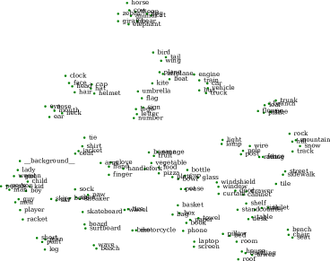
Figure 2: t-SNE visualization of the object classification weights that have been trained on top of contextualized image-based representations. Entities that appear similar to each other, or participate in similar relations, have a closer semantic affinity. This enables link prediction similar to Knowledge Graph Embeddings, and leads to generalization.

We train schemata using the Visual Genome (Krishna et al. 2017) dataset. We show that our model can accurately generate the captured commonsense knowledge and that iterative injection of this knowledge leads to significantly higher classification accuracy. Additionally, we draw from the recent advancements in self-supervised learning and show that the schemata can be trained with only a fraction of labeled images. This allows us to fine-tune the perception model without any additional images; instead, we can use a knowledge base of hand-crafted or external triples and train with their mental images (schemata). As a result, compared to the self-supervised baseline, and with 1% of the training data, our model achieves more than 3% improvement in object classification, 26% in scene graph classification, and 36% in predicate prediction; an accuracy that is almost equal to when using 100$\%$ of the labeled images.

Related Works

While the concept of schemata can be applied to any form of perceptual processing, and there are recent deep learning models of action schemata (Kansky et al. 2017; Goyal et al. 2020), we focus on the figurative schemata in the visual scene understanding domain. Even though there has been a body of related research outside the scene graph domain (Wu, Lenz, and Saxena 2014; Deng et al. 2014; Hu et al. 2016, 2017; Santoro et al. 2017), research in this field was accelerated mainly after the release of Visual Relation Detection (VRD) (Lu et al. 2016) and the Visual Genome (Krishna et al. 2017) datasets.  Baier, Ma, and Tresp (2017, 2018) proposed the first KG-based model of prior knowledge that improves SG classification. VTransE (Zhang et al. 2017) proposed to capture relations by applying the KGE model of TransE (Bordes et al. 2013) on the visual embeddings. Yu et al. (2017) employed a teacher-student model to distill external language knowledge. Iterative Message Passing (Xu et al. 2017), Neural Motifs (Zellers et al. 2018) (NM), and Graph R-CNN (Yang et al. 2018) used RNNs and graph convolutions to propagate image context. Tang et al. (2019) exploited dynamic tree structures and Chen et al. (2019a) proposed a method based on multi-agent policy gradients. Sharifzadeh et al. (2019) employed the predicted pseudo depth maps of the images in addition to the 2D information. In general, scene graph classification methods are closely related to KGE models (Nickel, Tresp, and Kriegel 2011; Nickel et al. 2016). For an extensive discussion on the connection between perception, KG models, and cognition, refer to (Tresp, Sharifzadeh, and Konopatzki 2019; Tresp et al. 2020). The link prediction in KGEs arises from the compositionality of the trained embeddings. Other forms of compositionality in neural networks are discussed in other works such as (Montufar et al. 2014). In this work, we introduce assimilation, which strengthens the representations within the neural network’s causal structure, addressing an issue of neural networks raised by Fodor, Pylyshyn et al. (1988). In general, some of the shortcomings that we address in this work have been recently argued by  Bengio (2017); Marcus (2018).

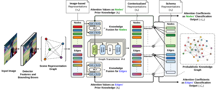
Figure 3: We formulate the classification as attention layer between object and schema representations. Contextualizing image-based object representations before classification encourages the schemata to learn image-based relational prior knowledge. As a result, the attention values that are injected from the schemata to scene representations and then propagated. In this way, they enrich the image-based representations with prior knowledge. Additionally, the interactions between schemata can reconstruct the probabilistic knowledge graph (right).

Methods

In this section we describe our method. In summary, after an initial classification step, we combine the image-based representations with the schema of their predicted class. We then proceed by contextualizing these representations and collecting supportive evidence from neighbors before re-classifying each entity (Ref. Figure 1). In what follows, bold lower case letters denote vectors, bold upper case letters denote matrices, and the letters denote scalar quantities or random variables. We use subscripts and superscripts to denote variables and calligraphic upper case letters for sets.

Definitions

Let us consider a given image $\mathbf{I}$ and a set of $n$ bounding boxes $\mathcal{B}=\{\mathbf{b}_{i}\}_{i=1}^{n}$, $\mathbf{b}_{i}=[b^{x}_{i},b^{y}_{i},b^{w}_{i},b^{h}_{i}]$, such that $[b^{x}_{i},b^{y}_{i}]$ are the coordinates of $\mathbf{b}_{i}$ and $[b^{w}_{i},b^{h}_{i}]$ are its width and height. We build a Scene Representation Graph, $\textit{SRG}=\{\mathcal{V},\mathcal{E}\}$ as a structured presentation of the objects and predicates in $\mathbf{I}$. $\mathcal{X}^{o}=\{\mathbf{x}_{i}^{o}\}_{i=1}^{n}$, $\mathbf{x}^{o}_{i}\in\mathbb{R}^{d}$ denote the features of object nodes and $\mathcal{X}^{p}=\{\mathbf{x}_{i}^{p}\}_{i=1}^{m}$, $\mathbf{x}^{p}_{i}\in\mathbb{R}^{d}$ denote the features of predicate nodes. Each $\mathbf{x}^{o}_{i}$ is initialized by a pooled image-based object representation, extracted by applying VGG16 (Simonyan and Zisserman 2014) or ResNet-50 (He et al. 2016) on the image contents of $\mathbf{b}_{i}$. Each $\mathbf{x}^{p}_{i}$ is initialized by applying a two layered fully connected network on the relational position vector $\mathbf{t}$ between a head $i$ and a tail $j$ where $\mathbf{t}=[t_{x},t_{y},t_{w},t_{h}]$, $t_{x}=(b^{x}_{i}-b^{x}_{j})/{b^{w}_{i}}_{j},t_{y}=(b^{y}_{i}-b^{y}_{j})/b^{h}_{j},t_{w}=\log(b^{w}_{i}/b^{w}_{j}),t_{h}=\log(b^{h}_{i}/b^{h}_{j})$. The implementation details of the networks are provided in the Supplementary.

Scene graph classification is the mapping of each node in scene representation graph to a label where each object node is from the label set $\mathcal{C}^{o}$ and each predicate node from $\mathcal{C}^{p}$. The resulting labeled graph is a set of triples referred to as the Scene Graph. We also define a Probabilistic Knowledge Graph (PKG) as a graph where the weight of a triple is the expected value of observing that relation given the head and tail classes and regardless of any given images. Later we will show that our model can accurately generate the PKG, i.e., the commonsense that is captured from perceptions during training.

In what comes next, $\mathbf{x}^{o}_{i}$ and $\mathbf{x}^{p}_{i}$ are treated identically except for classification with respect to $\mathcal{C}^{o}$ or $\mathcal{C}^{p}$. Therefore, for a better readability, we only write $\mathbf{x}_{i}$.

Contextualized Scene Representation Graph

We obtain contextualized object representations $\mathbf{z}_{i}$ by applying a graph convolutional neural network, on SRG. We sometimes refer to this module as our interaction function. We use a Graph Transformer as a variant of the Graph Network Block (Battaglia et al. 2018; Koncel-Kedziorski et al. 2019) with multi-headed attentions as

$$\mathbf{m}_{i}^{\mathcal{N}(i)}=\frac{1}{K}\sum_{k=1}^{K}\sum_{j\in\mathcal{N}(i)}\alpha_{ij}^{(l,k)}\mathbf{W}^{(l,k)}\mathbf{z}^{(l,t)}_{j}$$ (1)

$${\mathbf{z}^{\prime}}_{i}^{(l)}=\textit{LN}(\mathbf{z}^{(l,t)}_{i}+\mathbf{m}_{i}^{\mathcal{N}_{in}(i)}+\mathbf{m}_{i}^{\mathcal{N}_{out}(i)})$$ (2)

$$\mathbf{z}_{i}^{(l+1,t)}=\textit{LN}({\mathbf{z}^{\prime}}_{i}^{(l)}+f({\mathbf{z}^{\prime}}_{i}^{(l)})),$$ (3)

where $\mathbf{z}_{i}^{(l,t)}$ is the embedding of node $i$ in the $l$-th graph convolution layer and $t$-th assimilation. In the first layer $\mathbf{z}_{i}^{(0,t)}=\mathbf{x}_{i}$. LN is the layer norm (Ba, Kiros, and Hinton 2016), $K$ is the number of attentional heads and $\mathbf{W}^{(l,k)}$ is the weight matrix of the $k$-th head in layer $l$. $\mathcal{N}(i)$ represent the set of neighbors, which are either incoming ${\mathcal{N}_{in}(i)}$ or outgoing $\mathcal{N}_{out}(i)$. $f(.)$ is a two layered feed-forward neural network with Leaky ReLU non-linearities between each layer. $\alpha_{ij}^{(l,k)}$ denotes the attention coefficients in each head and is defined as

$$e_{ij}^{(l,k)} =\sigma(\mathbf{h}^{(l,k)}\cdot[\mathbf{z}_{i}^{(l)}||\mathbf{W}^{(l,k)}\mathbf{z}^{(l)}_{j}])$$ (4)

$$\alpha_{ij}^{(l,k)} =\frac{\exp(e_{ij}^{(l,k)})}{\sum_{q\in\mathcal{N}(i)}\exp(e_{iq}^{(l,k)})}$$ (5)

with $\mathbf{h}^{(l,k)}$ as a learnable weight vector and $||$ denoting concatenation. $\sigma$ is the Leaky ReLU with the slope of $0.2$.

Schemata

We define the schema of a class $c$ as an embedding vector $\mathbf{s}_{c}$. We realize object and predicate classification by an attention layer between the contextualized representations and the schemata such that the classification outputs $\alpha^{\prime}_{ic}$ are computed as the attention coefficients between $\mathbf{z}_{i}$ and $\mathbf{s}_{c}$ as

$$\alpha^{\prime}_{ic}=\mathrm{softmax}(a(\mathbf{z}_{i}^{(L,t)},\mathbf{s}_{c}))$$ (6)

where, $a(.)$ is the attention function that we implement as the dot-product between the input vectors, and $\mathbf{z}_{i}^{(L,t)}$ is the output from the last ($L$-th) layer of the Graph Transformer. The attention values $\bm{\delta}_{i}$ capture the schemata messages as

$$\bm{\delta}_{i}=\sum_{c\in\mathcal{C}}\alpha^{\prime}_{ic}\mathbf{s}_{c}$$ (7)

and we inject them back to update the scene representations as

$$\mathbf{u}_{i}=\textit{LN}(\mathbf{x}_{i}+\bm{\delta}_{i})$$ (8)

$$\mathbf{z}_{i}^{(0,t+1)}=\textit{LN}(\mathbf{u}_{i}+g(\mathbf{u}_{i}))$$ (9)

where $g(.)$ is a two-layered feed-forward network with Leaky ReLU non-linearities. Note that we compute $\mathbf{u}_{i}$ by fusing the attention values with the original image features $\mathbf{x}_{i}$. Therefore, the outputs from previous Graph Transformer layers will not be accumulated, and the original image-based features will not vanish.

We define assimilation as the set of computations from $\mathbf{z}_{i}^{(L,t)}$ to $\mathbf{z}_{i}^{(L,t+1)}$. This includes the initial classification step (Eq. 6), fusion of schemata with image-based vectors (Eq. 9) and the application of the interaction function on the updated embeddings (Eq. 3). We expect to get refined object representations after the assimilation. Therefore, we assimilate several times such that after each update of the classification results, the priors are also updated accordingly. During training, and for each step of assimilation, we employ a supervised attention loss, i.e. categorical cross entropy, between the one-hot encoded ground truth labels and $\alpha^{\prime}_{ic}$. This indicates a multi-task learning strategy where one task (for the first assimilation) is to optimize for $P(y_{q}|x_{1},...,x_{\theta})$, with $x_{q}$ as a random variable representing the image-based features of $q$, $y_{q}$ as the label, and $\theta=m+n$. The other set of tasks is to optimize for $P(y^{t+1}_{q}|x^{t}_{1},...,x^{t}_{\theta},y^{t}_{1},...,y^{t}_{\theta})$. We refer to the first task as IC, for Image-based Classification and to the second set of tasks as ICP for Image-based Classification with Prior knowledge. Note that even when no images are available, we can still train for the ICP from a collection of external or hand-crafted triples by setting $\mathbf{x}_{i}=\vec{0}$, $\alpha^{\prime}_{ic}=onehot(c_{i})$, and starting from Eq 7. When we solve for both tasks, to stabilize the training, such that it does not diverge in the early steps (when the predictions are noisy), we train our model by a modified form of scheduled sampling (Bengio et al. 2015) such that in Eq 7, we gradually replace up to $10$ percent of the randomly sampled false negative predictions $\alpha^{\prime}$ with the their true labels. This prevents the model to over-fit a specific error rate from a previous assimilation, and encourages it to generalize beyond the number of assimilations that it has been trained for.

GCN vs. Prior Model: A matter of inductive biases

Typical GCNs, such as the Graph Transformer, take the features derived from each bounding box as input, apply non-linear transformations and propagate them to the neighbors in the following layers. Each GCN layer consists of fully connected neural networks. Therefore, theoretically they can also model and propagate prior knowledge that is not visible in bounding boxes. However, experimental results of previous works (and also this work) confirm that explicit modeling and propagation of prior knowledge (ICP) can still improve the classification accuracy. Why is that the case?

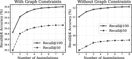
Figure 4: The results of our ablation studies. We study the effect of each assimilation in scene graph classification. Note that the model has been trained for only 4 assimilations yet it can generalize, thanks to the scheduled sampling strategy.

Let us consider the following. According to the the universal approximation theorem (Csáji et al. 2001), when we solve for IC as $P(y_{k}|x_{1},...,x_{o})$, our model might learn to capture a desired form of $P(y_{k}|x_{1},...,x_{o},y_{1},...,y_{o})$. However, in practice, the learning algorithm does not always find the best function. Therefore, we require the proper inductive biases to guide us through the learning process. As  Caruana (1997) puts: ”Multitask Learning is an approach to inductive transfer that improves generalization by using the domain information contained in the training signals of related tasks as an inductive bias. It does this by learning tasks in parallel while using a shared representation; what is learned for each task can help other tasks be learned better”. For example, in the encoder-decoder models for machine translation e.g. Transformers (Vaswani et al. 2017), the prediction is often explicitly conditioned not just on the encoded inputs but also on the decoded outputs of the previous tokens. Therefore, the decoding in each step can be interpreted as $P(y_{k}|x_{1},...,x_{o},y_{1},...,y_{k-1})$. Note that the previous predictions such as $y_{1}$, cannot benefit from the future predictions $\{y_{2},...,y_{o}\}$. However, in our model, we provide an explicit bias towards utilizing predictions in all indices. In fact, our model can be interpreted as an encoder-decoder network, where the decoder consists of multiple decoders. Therefore, the decoding depends not just on the encoded image features but also on the previously decoded outputs. In other words, by injecting schema embeddings, as embeddings that are trained over all images, we impose the bias to propagate what is not visible in the bounding box. As will be shown later, we can train for ICP and IC even with smaller splits of annotated images, which can lead to competitive results with fewer labels. Additionally, assimilation enables us to quantify the propagated prior knowledge. This interpretability is another advantage that GCNs alone do not have.

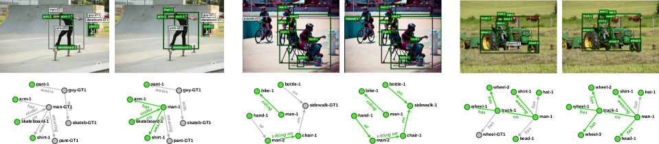
Figure 5: Qualitative examples of improved scene graph classification results (Recall@50) through assimilations of our model. From left to right is after each assimilation. Green and gray colors indicate true positives and false negatives concluded by the model. For example consider the middle image, where the sidewalk was initially misclassified as a street. After seeing a biker in the image and a man sitting on a chair, a reasonable inference is that this should be a sidewalk.

Backbone	Main Model	SGCls R@100			PredCls R@100			Object Classification
		$1{\%}$	$10{\%}$	$100{\%}$	$1{\%}$	$10{\%}$	$100{\%}$	$1{\%}$	$10{\%}$	$100{\%}$
Supervised	IC	$\phantom{0}1.84$ $\pm 0.26$	$13.90$ $\pm 0.97$	$33.6$	$40.61$ $\pm 0.84$	$52.51$ $\pm 1.19$	$62.0$	$14.38$ $\pm 0.57$	$38.45$ $\pm 1.21$	$64.2$
Self-Supervised	IC	$12.12$ $\pm 0.47$	$26.14$ $\pm 0.77$	$36.8$	$48.10$ $\pm 0.54$	$58.14$ $\pm 0.35$	$63.4$	$40.75$ $\pm 0.48$	$56.97$ $\pm 0.76$	$68.0$
Self-Supervised	IC + ICP	$15.36$ $\pm 0.38$	$27.37$ $\pm 0.47$	$37.1$	$65.68$ $\pm 0.12$	$65.42$ $\pm 0.19$	$65.7$	$42.09$ $\pm 0.65$	$58.60$ $\pm 0.56$	$68.4$

Table 1: Comparison of R@100 for SGCls, PredCls and Object Classification tasks on smaller splits of the VG dataset.

	Method	SGCls		PredCls
		R@50	R@100	R@50	R@100	Mean
Unconstrained	IMP+ (Xu et al. 2017)	$43.4$	$47.2$	$75.2$	$83.6$	$62.3$
	FREQ (Zellers et al. 2018)	$40.5$	$43.7$	$71.3$	$81.$2	$59.1$
	SMN (Zellers et al. 2018)	$44.5$	$47.7$	$81.1$	$88.3$	$65.4$
	KERN(Chen et al. 2019c)	$45.9$	$49.0$	$81.9$	$88.9$	$66.4$
	CCMT(Chen et al. 2019a)	$48.6$	$52.0$	$83.2$	$90.1$	$68.4$
	Schemata	$48.5$	$52.1$	$83.8$	$90.5$	$68.7$
Constrained	VRD (Lu et al. 2016)	$11.8$	$14.1$	$27.9$	$35.0$	$22.2$
	IMP (Xu et al. 2017)	$21.7$	$24.4$	$44.8$	$53.0$	$36.9$
	IMP+ (Xu et al. 2017)	$34.6$	$35.4$	$59.3$	$61.3$	$47.6$
	FREQ (Zellers et al. 2018)	$32.4$	$34.0$	$59.9$	$64.1$	$47.6$
	SMN (Zellers et al. 2018)	$35.8$	$36.5$	$65.2$	$67.1$	$51.1$
	KERN(Chen et al. 2019c)	$36.7$	$37.4$	$65.8$	$67.6$	$51.8$
	VCTree(Tang et al. 2019)	$38.1$	$38.8$	$66.4$	$68.1$	$52.8$
	CCMT(Chen et al. 2019a)	$39.0$	$39.8$	$66.4$	$68.1$	$53.3$
	Schemata	$39.1$	$39.8$	$66.9$	$68.4$	$53.5$
	Schemata - PKG	–.-	–.-	$48.9$	$54.2$	–.-

Table 2: Comparison of the R@50 and R@100, with and without graph constraints for SGCls and PredCls tasks on the VG dataset.

Evaluation

	Method	SGCls		PredCls
		mR@50	mR@100	mR@50	mR@100	Mean
Unconstrained	IMP+ (Xu et al. 2017)	$12.1$	$16.9$	$20.3$	$28.9$	$19.5$
	FREQ (Zellers et al. 2018)	$13.5$	$19.6$	$24.8$	$37.3$	$23.8$
	SMN (Zellers et al. 2018)	$15.4$	$20.6$	$27.5$	$37.9$	$25.3$
	KERN(Chen et al. 2019c)	$19.8$	$26.2$	$36.3$	$49.0$	$32.8$
	Schemata	$21.4$	$28.8$	$40.1$	$54.9$	$36.3$
Constrained	IMP (Xu et al. 2017)	$\phantom{0}3.1$	$\phantom{0}3.8$	$\phantom{0}6.1$	$\phantom{0}8.0$	$\phantom{0}5.2$
	IMP+ (Xu et al. 2017)	$\phantom{0}5.8$	$\phantom{0}6.0$	$\phantom{0}9.8$	$10.5$	$\phantom{0}8.0$
	FREQ (Zellers et al. 2018)	$\phantom{0}6.8$	$\phantom{0}7.8$	$13.3$	$15.8$	$10.9$
	SMN (Zellers et al. 2018)	$\phantom{0}7.1$	$\phantom{0}7.6$	$13.3$	$14.4$	$10.6$
	KERN(Chen et al. 2019c)	$\phantom{0}9.4$	$10.0$	$17.7$	$19.2$	$14.0$
	VCTree(Tang et al. 2019)	$10.1$	$10.8$	$17.9$	$19.4$	$14.5$
	Schemata	$10.1$	$10.9$	$19.1$	$20.7$	$15.2$
	Schemata - PKG	–.-	–.-	$\phantom{0}8.2$	$\phantom{0}9.4$	–.-

Table 3: Comparison of the mR@50 and mR@100, with and without graph constraints for SGCls and PredCls tasks on the VG dataset.

Settings

We train our models on the common split of Visual Genome (Krishna et al. 2017) dataset containing images labeled with their scene graphs (Xu et al. 2017). This split takes the most frequent 150 object and 50 predicate classes in total, with an average of 11.5 objects and 6.2 predicates in each image. We report the experimental results on the test set, under two standard classification settings of predicate classification (PredCls): predicting predicate labels given a ground truth set of object boxes and object labels, and scene graph classification (SGCls): predicting object and predicate labels, given the set of object boxes. Another popular setting is the scene graph detection (SGDet), where the network should also detect the bounding boxes. Since the focus of our study is not on improving the object detector backbone and our improvements in SGDet are similar to the improvements in SGCls, we do not report them here. For those results, please refer to our official code repository. We report the results of these settings under constrained and unconstrained setups (Yu et al. 2017). In the unconstrained setup, we allow for multiple predicate labels, whereas in the constrained setup, we only take the top-1 predicted predicate label.

Metrics

We use Recall@K (R@K) as the standard metric. R@K computes the mean prediction accuracy in each image given the top $K$ predictions. In VG, the distribution of labeled relations is highly imbalanced. Therefore, we additionally report Macro Recall (Sharifzadeh et al. 2019; Chen et al. 2019c) (mR@K) to reflect the improvements in the long tail of the distribution. In this setting, the overall recall is computed by taking the mean over recall per predicate.

Experiments

The goal of our experiments is (A) to study whether injecting prior knowledge into scene representations can improve the classification and (B) to study the commonsense knowledge that is captured in our model. In what follows, backbone refers to VGG16/ResNet-50 that generates the SRG, and main model refers to part of the network that applies contextualization and assimilation. The backbone can be trained from a set of labeled images (in a supervised manner), unlabeled images (in a self-supervised manner), or a combination of the two. The main model can be trained from a set of labeled images (the IC task), a prior knowledge base (ICP) or a combination of the two. Note that the memory consumption of the model is in the same order as Graph R-CNN and computing the extra attention heads can also be further optimized by estimating the softmax kernels (Choromanski et al. 2020). For (A), we conduct the following studies:

1. We train both the backbone and the main model from all the labeled images and for both tasks. We use the VGG-16 backbone as trained by Zellers et al. (2018). This allows us to compare the results with the related works directly. We evaluate the classification accuracy for 8 assimilations (until the changes are not significant anymore). Table 2 and 3 compare the performance of our model to the state-of-the-art. As shown, our model exceeds the others on average and under most settings. Figure 4 shows our ablation study, indicating that the accuracy is improved after each assimilation.

2. To qualitatively examine these results, we present some of the images and their scene graphs after two assimilations, in Figure 5. For example in the right image, while the wheel is almost fully occluded, we can still classify it once we classify other objects and employ commonsense (e.g., trucks have wheels). Another interesting example is the middle image, where the sidewalk is initially misclassified as a street. After seeing a biker in the image and a man sitting on a chair, a reasonable inference is that this should be a sidewalk! Similarly, in the left image, the man is facing away from the camera, and his pose makes it hard to classify him unless we utilize our prior knowledge about the arm, pants, shirt, and skateboard.

3. Figure 7 shows the improvements per each predicate class. The results indicate that most improvements occur in under-represented classes. This means that we have achieved a generalization performance that is beyond the simple reflection of the dataset’s statistical bias.

4. To understand the importance of prior knowledge compared to having a large set of labeled images, we conduct the following study: we uniformly sample two splits with $1\%$ and $10\%$ of VG. The images in each split are considered as labeled. We ignore the labels of the remaining images and consider them as unlabeled. Instead, we treat the set of ignored labels as a form of external/hand-crafted knowledge in the form of triples. For each split, we train the full model (i@) with a backbone that has been trained in a supervised fashion with the respective split and no pre-training, and the main model that has been trained for IC (without commonsense) with the respective split, (ii@) with a backbone that has been pre-trained on ImageNet (Deng et al. 2009) and fine-tuned on the Visual Genome (in a self-supervised fashion with BYOL (Grill et al. 2020)) and fine-tuned on the respective split of the visual genome (in a supervised fashion) and the main model that has been trained for IC with the respective split, and (iii@) Similar to 2, except that we include the ICP and train the main model by assimilating the entire prior knowledge base including the external triples. We discard their image-based features ($\mathbf{x}_{i}$) for the triples outside a split. Since BYOL is based on ResNet-50, for a fair comparison, we train all models in this experiment with ResNet-50 (including another model that we train with $100\%$ of the data). In the Scene Graph Classification community, the results are often reported under an arbitrary random seed, and previous works have not reported the summary statistics over several runs before. To allow for a fair comparison of our model to those works (on the $100\%$ set), we followed the same procedure in the study A1. However, to encourage a statistically more stable comparison of future models in this experiment, we report the summary statistics (arithmetic mean and standard deviation) over five random fractions ($1\%$ and $10\%$) of VG training set. As shown in Table 1, utilizing prior knowledge allows to achieve almost the same predicate prediction accuracy with $1\%$ of the data only. Also, we largely improve object classification and scene graph classification.

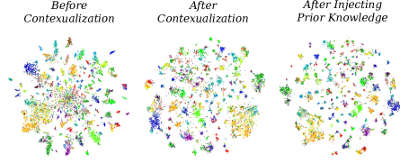
Figure 6: t-SNE visualization of object representations before contextualization, after contextualization and after injecting prior knowledge.

For B we consider the following studies:

1. We visualize the semantic affinity of schema representations by employing t-SNE (Maaten and Hinton 2008). As we can see in Figure 2, the schema representations of entities that are visually or relationally similar are the closest to each other.

2. We inspect the semantic affinity of object representations by employing t-SNE (i@) before contextualization, (ii@) after contextualization and (iii@) after injecting prior knowledge. The results are represented in Figure 6. Each color represents a different object class. This investigation confirms that object representations will get into more separable clusters after injecting prior knowledge.

3. Finally, we evaluate our model’s accuracy in link prediction. The goal is to quantitatively evaluate our model’s understanding of relational commonsense, i.e., relational structure of the probabilistic knowledge graph. Similar to a KGE link prediction, we predict the predicate given head and tail of a relation. In other words, we feed our model with the schema of head and tail, together with a zero-vector for the image-based representations. As we can see in Table 3 & 2, in Schemata - PKG, even if we do not provide any image-based information, our model can still guess the expected predicates similar to a KGE model. While this guess is not as accurate as when we present it with an image, the accuracy is still remarkable.

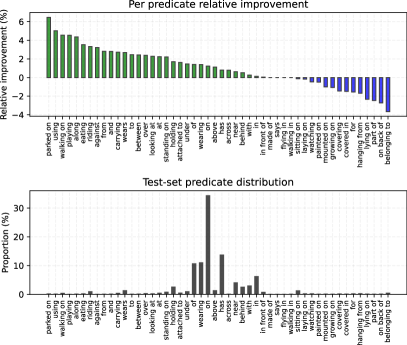
Figure 7: The top plot shows the per predicate classification accuracy improvement, in SGCls R@100 with no graph constraints and from Assimiliation 1 to Assimilation 8. The bottom plot shows the distribution of sample proportion for the predicates in Visual Genome.

Conclusion

We discussed schemata as mental representations that enable compositionality and reasoning. To model schemata in a deep learning framework, we introduced them as representations that encode image-based and relational prior knowledge of objects and predicates in each class. By defining classification as an attention layer instead of a fully connected layer, we introduced an inductive bias that enabled the propagation of prior knowledge. Our experiments on the Visual Genome dataset confirmed the effectiveness of assimilation through qualitative and quantitative measures. Our model achieved higher accuracy under most settings and could also accurately predict the commonsense knowledge. Additionally, we showed that our model could be fine-tuned from external sources of knowledge in the form of triples. When combined with pre-trained schemata in a self-supervised setting, this leads to a predicate prediction accuracy that is almost equal to the full model. Also, it gives significant improvements in the scene graph and object classification tasks. We hope that this work will open new research directions in utilizing commonsense to learn from little annotations.

Appendix A Architectural Details

As discussed before, for the experiments A1-3, similar to  (Zellers et al. 2018) and following works, we use Faster R-CNN (Ren et al. 2015) with VGG-16 (Simonyan and Zisserman 2014) and for the A4, we use ResNet-50. After extracting the image embeddings from the penultimate fully connected (fc) layer of the backbones, we feed them to a fc-layer with 512 neurons and a Leaky ReLU with a slope of 0.2, together with a dropout rate of 0.8. This gives us initial object node embeddings. We apply a fc-layer with 512 neurons and Leaky ReLU with a slope 0.2 and dropout rate of 0.1, to the extracted spatial vector $\mathbf{t}$ to initialize predicate embeddings. For the contextualization, we take four graph transformer layers of 5 heads each. $f$ and $g$ have 2048 and 512 neurons in each layer. We initial the layers with using Glorot weights (Glorot and Bengio 2010).

Appendix B Training with Full Data (A1-3)

We trained our full model for SGCls setting with Adam optimizer (Kingma and Ba 2014) and a learning rate of $10^{-5}$ for 24 epochs with a batch size of 14. We fine-tuned this model for PredCls with 10 epochs, batchsize of 24, and SGD optimizer with learning rate of $10^{-4}$. We used an NVIDIA RTX-2080ti GPU for training.

Appendix C Training with Splits of Data (A4)

Training Details of the Backbones

Supervised:

We train the supervised backbones on the corresponding split of visual genome training set with the Adam optimizer (Kingma and Ba 2014) and a learning rate of $10^{-5}$ for 20 epochs with a batch size of 6.

Self-supervised:

We train the self-supervised backbones with the BYOL (Grill et al. 2020) approach. We fine-tune the pre-trained self-supervised weights over ImageNet (Deng et al. 2009), on the entire training set of Visual Genome images in a self-supervised manner with no labels, for 3 epochs with a batch-size of 6, SGD optimizer with a learning rate of $6\times 10^{-5}$, momentum of 0.9 and weight decay of $4\times 10^{-4}$. Similar to BYOL, we use a MLP hidden size of 512 and a projection layer size of 128 neurons. Then for each corresponding split, we fine-tune the weights in a supervised manner with the Adam optimizer and a learning rate of $10^{-5}$ for 4 epochs with a batch size of 6.

Training Details of the Main Models

Supervised + IC

We train the main model with the Adam optimizer and a learning rate of $10^{-5}$ and a batch size of 22, with 5 epochs for the $1\%$ and 11 epochs for $10\%$.

Self-supervised + IC

We train the main model with the Adam optimizer and a learning rate of $10^{-5}$ and a batch size of 22, with 6 epochs for the $1\%$ and 11 epochs for $10\%$.

Self-supervised + IC + ICP

We train the main model with the Adam optimizer and a learning rate of $10^{-5}$ with a batch size of 16, with 6 epochs for the $1\%$ and 11 epochs for $10\%$. We train these models with 2 assimilations.

Appendix D Additional Qualitative Results

In Figure 11 and 12, we present additional qualitative results on the Assimilation Study (Figure 4, Table 1 and Table 2 in the main paper). In each assimilation either object or predicate classification are improved.

Appendix E Per-predicate Improvement

In the main paper, we reported the per-predicate improvement of assimilation 1 to 8 in SGCls, under the R@100, and in the unconstrained setting. Here we present the additional results under R@50 and also in the constrained settings in Figure 8, 9 and 10. The predicate statistics in all settings are the same and equal to the reported statistics in the main paper (Figure 7). Therefore, to avoid repeating the statistics under each plot and have a more visually appealing design, we embed these statistics as the brightness level of the bar colors. The darker shades indicate larger statistics and the lighter shades indicate smaller statistics. As we can see, most improvements occur in under-represented predicate classes.

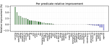
Figure 8: R@50 - with graph constraints

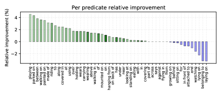
Figure 9: R@50 - with no graph constraints

Figure 10: R@100 - with graph constraints

	Method	Main Model	R@50		R@100
			$1{\%}$	$10{\%}$	$1{\%}$	$10{\%}$
SGCls	Supervised	IC	$\phantom{0}1.98\pm 0.28$	$16.24\pm 1.13$	$\phantom{0}2.40\pm 0.30$	$18.15\pm 1.23$
	Self-Supervised	IC	$13.34\pm 0.51$	$30.45\pm 0.95$	$15.75\pm 0.64$	$33.94\pm 0.94$
	Self-Supervised	IC + ICP	$\mathbf{17.54\pm 0.43}$	$\mathbf{31.72\pm 0.61}$	$\mathbf{19.59\pm 0.49}$	$\mathbf{35.33\pm 0.65}$
PredCls	Supervised	IC	$42.46\pm 0.99$	$60.21\pm 0.93$	$55.08\pm 1.10$	$71.87\pm 0.84$
	Self-Supervised	IC	$51.77\pm 0.59$	$65.89\pm 0.42$	$63.64\pm 0.75$	$76.85\pm 0.38$
	Self-Supervised	IC + ICP	$\mathbf{73.89\pm 0.19}$	$\mathbf{73.25\pm 0.23}$	$\mathbf{84.30\pm 0.16}$	$\mathbf{83.69\pm 0.20}$

Table 4: Comparison of R@50 and R@100 with no graph constraints, for SGCls and PredCls tasks on the provided VG splits.

	Method	Main Model	mR@50		mR@100
			$1{\%}$	$10{\%}$	$1{\%}$	$10{\%}$
SGCls	Supervised	IC	$0.29\pm 0.07$	$4.65\pm 0.62$	$0.43\pm 0.10$	$\phantom{0}6.72\pm 0.77$
	Self-Supervised	IC	$2.54\pm 0.42$	$9.93\pm 0.35$	$3.71\pm 0.49$	$13.89\pm 0.51$
	Self-Supervised	IC + ICP	$\mathbf{4.84\pm 0.13}$	$\mathbf{9.94\pm 0.54}$	$\mathbf{6.83\pm 0.16}$	$\mathbf{14.11\pm 0.64}$
PredCls	Supervised	IC	$\phantom{0}5.89\pm 0.26$	$15.02\pm 1.37$	$\phantom{0}9.62\pm 0.38$	$23.22\pm 1.78$
	Self-Supervised	IC	$\phantom{0}9.24\pm 1.31$	$20.52\pm 0.53$	$14.28\pm 1.63$	$30.24\pm 0.72$
	Self-Supervised	IC + ICP	$\mathbf{27.11\pm 0.44}$	$\mathbf{25.76\pm 0.74}$	$\mathbf{40.35\pm 0.77}$	$\mathbf{38.48\pm 0.82}$

Table 5: Comparison of mR@50 and mR@100 with no graph constraints, for SGCls and PredCls tasks on the provided VG splits.

	Method	Main Model	R@50		R@100
			$1{\%}$	$10{\%}$	$1{\%}$	$10{\%}$
SGCls	Supervised	IC	$\phantom{0}1.65\pm 0.26$	$13.37\pm 0.94$	$\phantom{0}1.84\pm 0.26$	$13.90\pm 0.97$
	Self-Supervised	IC	$11.19\pm 0.41$	$25.16\pm 0.79$	$12.12\pm 0.47$	$26.14\pm 0.77$
	Self-Supervised	IC + ICP	$\mathbf{14.72\pm 0.38}$	$\mathbf{26.33\pm 0.45}$	$\mathbf{15.36\pm 0.38}$	$\mathbf{27.37\pm 0.47}$
PredCls	Supervised	IC	$34.92\pm 0.81$	$48.69\pm 1.24$	$40.61\pm 0.84$	$52.51\pm 1.19$
	Self-Supervised	IC	$43.13\pm 0.59$	$54.40\pm 0.39$	$48.10\pm 0.54$	$58.14\pm 0.35$
	Self-Supervised	IC + ICP	$\mathbf{62.02\pm 0.10}$	$\mathbf{61.71\pm 0.19}$	$\mathbf{65.68\pm 0.12}$	$\mathbf{65.42\pm 0.19}$

Table 6: Comparison of R@50 and R@100 with graph constraints, for SGCls and PredCls tasks on the provided VG splits.

	Method	Main Model	mR@50		mR@100
			$1{\%}$	$10{\%}$	$1{\%}$	$10{\%}$
SGCls	Supervised	IC	$0.19\pm 0.04$	$2.21\pm 0.34$	$0.22\pm 0.04$	$2.43\pm 0.36$
	Self-Supervised	IC	$1.53\pm 0.20$	$\mathbf{5.31\pm 0.39}$	$1.71\pm 0.22$	$\mathbf{5.80\pm 0.40}$
	Self-Supervised	IC + ICP	$\mathbf{2.45\pm 0.05}$	$5.17\pm 0.23$	$\mathbf{2.68\pm 0.06}$	$5.68\pm 0.23$
PredCls	Supervised	IC	$\phantom{0}3.80\pm 0.20$	$\phantom{0}8.16\pm 0.67$	$\phantom{0}4.56\pm 0.22$	$\phantom{0}9.45\pm 0.76$
	Self-Supervised	IC	$\phantom{0}5.64\pm 0.56$	$11.35\pm 0.34$	$\phantom{0}6.61\pm 0.62$	$12.96\pm 0.32$
	Self-Supervised	IC + ICP	$\mathbf{14.80\pm 0.31}$	$\mathbf{14.59\pm 0.60}$	$\mathbf{17.06\pm 0.39}$	$\mathbf{16.92\pm 0.58}$

Table 7: Comparison of mR@50 and mR@100 with graph constraints, for SGCls and PredCls tasks on the provided VG splits.

Method	Main Model	Object Classification
		$1{\%}$	$10{\%}$
Supervised	IC	$14.38\pm 0.57$	$38.45\pm 1.21$
Self-Supervised	IC	$40.75\pm 0.48$	$56.97\pm 0.76$
Self-Supervised	IC + ICP	$\mathbf{42.09\pm 0.65}$	$\mathbf{58.60\pm 0.56}$

Table 8: Comparison of object classification accuracy (Top-1) on the provided VG splits.

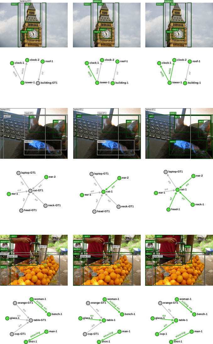
Figure 11: Qualitative examples of improved scene graph classification results (R@50 - with graph constraints) through assimilations of our model. From left to right is after each assimilation. Green and gray colors indicate true positives and false negatives concluded by the model.

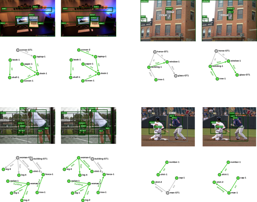
Figure 12: Qualitative examples of improved scene graph classification results (R@50 - with graph constraints) through assimilations of our model. From left to right is after each assimilation. Green and gray colors indicate true positives and false negatives concluded by the model.

References

- Arbib (1992) Arbib, M. A. 1992. Schema theory. The encyclopedia of artificial intelligence 2: 1427–1443.
- Ba, Kiros, and Hinton (2016) Ba, J. L.; Kiros, J. R.; and Hinton, G. E. 2016. Layer normalization. arXiv preprint arXiv:1607.06450 .
- Baier, Ma, and Tresp (2017) Baier, S.; Ma, Y.; and Tresp, V. 2017. Improving visual relationship detection using semantic modeling of scene descriptions. In International Semantic Web Conference, 53–68. Springer.
- Baier, Ma, and Tresp (2018) Baier, S.; Ma, Y.; and Tresp, V. 2018. Improving information extraction from images with learned semantic models. In Proceedings of the 27th International Joint Conference on Artificial Intelligence, 5214–5218. AAAI Press.
- Battaglia et al. (2018) Battaglia, P. W.; Hamrick, J. B.; Bapst, V.; Sanchez-Gonzalez, A.; Zambaldi, V.; Malinowski, M.; Tacchetti, A.; Raposo, D.; Santoro, A.; Faulkner, R.; et al. 2018. Relational inductive biases, deep learning, and graph networks. arXiv preprint arXiv:1806.01261 .
- Bengio et al. (2015) Bengio, S.; Vinyals, O.; Jaitly, N.; and Shazeer, N. 2015. Scheduled sampling for sequence prediction with recurrent neural networks. In Advances in Neural Information Processing Systems, 1171–1179.
- Bengio (2017) Bengio, Y. 2017. The consciousness prior. arXiv preprint arXiv:1709.08568 .
- Bordes et al. (2013) Bordes, A.; Usunier, N.; Garcia-Duran, A.; Weston, J.; and Yakhnenko, O. 2013. Translating embeddings for modeling multi-relational data. In Advances in neural information processing systems, 2787–2795.
- Caruana (1997) Caruana, R. 1997. Multitask learning. Machine learning 28(1): 41–75.
- Chen et al. (2019a) Chen, L.; Zhang, H.; Xiao, J.; He, X.; Pu, S.; and Chang, S.-F. 2019a. Counterfactual critic multi-agent training for scene graph generation. In Proceedings of the IEEE International Conference on Computer Vision, 4613–4623.
- Chen et al. (2019b) Chen, T.; Xu, M.; Hui, X.; Wu, H.; and Lin, L. 2019b. Learning semantic-specific graph representation for multi-label image recognition. In Proceedings of the IEEE International Conference on Computer Vision, 522–531.
- Chen et al. (2019c) Chen, T.; Yu, W.; Chen, R.; and Lin, L. 2019c. Knowledge-embedded routing network for scene graph generation. In Proceedings of the IEEE Conference on Computer Vision and Pattern Recognition, 6163–6171.
- Chen et al. (2019d) Chen, V. S.; Varma, P.; Krishna, R.; Bernstein, M.; Re, C.; and Fei-Fei, L. 2019d. Scene graph prediction with limited labels. In Proceedings of the IEEE International Conference on Computer Vision, 2580–2590.
- Choromanski et al. (2020) Choromanski, K.; Likhosherstov, V.; Dohan, D.; Song, X.; Gane, A.; Sarlos, T.; Hawkins, P.; Davis, J.; Mohiuddin, A.; Kaiser, L.; et al. 2020. Rethinking attention with performers. arXiv preprint arXiv:2009.14794 .
- Csáji et al. (2001) Csáji, B. C.; et al. 2001. Approximation with artificial neural networks. Faculty of Sciences, Etvs Lornd University, Hungary 24(48): 7.
- Deng et al. (2014) Deng, J.; Ding, N.; Jia, Y.; Frome, A.; Murphy, K.; Bengio, S.; Li, Y.; Neven, H.; and Adam, H. 2014. Large-scale object classification using label relation graphs. In European conference on computer vision, 48–64. Springer.
- Deng et al. (2009) Deng, J.; Dong, W.; Socher, R.; Li, L.-J.; Li, K.; and Fei-Fei, L. 2009. Imagenet: A large-scale hierarchical image database. In 2009 IEEE conference on computer vision and pattern recognition, 248–255. Ieee.
- Fodor, Pylyshyn et al. (1988) Fodor, J. A.; Pylyshyn, Z. W.; et al. 1988. Connectionism and cognitive architecture: A critical analysis. Cognition 28(1-2): 3–71.
- Glorot and Bengio (2010) Glorot, X.; and Bengio, Y. 2010. Understanding the difficulty of training deep feedforward neural networks. In Proceedings of the thirteenth international conference on artificial intelligence and statistics, 249–256.
- Goyal et al. (2020) Goyal, A.; Lamb, A.; Gampa, P.; Beaudoin, P.; Levine, S.; Blundell, C.; Bengio, Y.; and Mozer, M. 2020. Object Files and Schemata: Factorizing Declarative and Procedural Knowledge in Dynamical Systems. arXiv preprint arXiv:2006.16225 .
- Grill et al. (2020) Grill, J.-B.; Strub, F.; Altché, F.; Tallec, C.; Richemond, P. H.; Buchatskaya, E.; Doersch, C.; Pires, B. A.; Guo, Z. D.; Azar, M. G.; et al. 2020. Bootstrap your own latent: A new approach to self-supervised learning. arXiv preprint arXiv:2006.07733 .
- He et al. (2016) He, K.; Zhang, X.; Ren, S.; and Sun, J. 2016. Deep residual learning for image recognition. In Proceedings of the IEEE conference on computer vision and pattern recognition, 770–778.
- Hochreiter and Schmidhuber (1997) Hochreiter, S.; and Schmidhuber, J. 1997. Long short-term memory. Neural computation 9(8): 1735–1780.
- Hou et al. (2019) Hou, J.; Wu, X.; Qi, Y.; Zhao, W.; Luo, J.; and Jia, Y. 2019. Relational Reasoning using Prior Knowledge for Visual Captioning. arXiv preprint arXiv:1906.01290 .
- Hu et al. (2017) Hu, H.; Deng, Z.; Zhou, G.-T.; Sha, F.; and Mori, G. 2017. Labelbank: Revisiting global perspectives for semantic segmentation. arXiv preprint arXiv:1703.09891 .
- Hu et al. (2016) Hu, H.; Zhou, G.-T.; Deng, Z.; Liao, Z.; and Mori, G. 2016. Learning structured inference neural networks with label relations. In Proceedings of the IEEE Conference on Computer Vision and Pattern Recognition, 2960–2968.
- Kansky et al. (2017) Kansky, K.; Silver, T.; Mély, D. A.; Eldawy, M.; Lázaro-Gredilla, M.; Lou, X.; Dorfman, N.; Sidor, S.; Phoenix, S.; and George, D. 2017. Schema networks: Zero-shot transfer with a generative causal model of intuitive physics. arXiv preprint arXiv:1706.04317 .
- Kant (1787) Kant, I. 1787. Kritik der reinen Vernunft:[Hauptband]. Walter de Gruyter.
- Kingma and Ba (2014) Kingma, D. P.; and Ba, J. 2014. Adam: A method for stochastic optimization. arXiv preprint arXiv:1412.6980 .
- Kipf and Welling (2016) Kipf, T. N.; and Welling, M. 2016. Semi-supervised classification with graph convolutional networks. arXiv preprint arXiv:1609.02907 .
- Koncel-Kedziorski et al. (2019) Koncel-Kedziorski, R.; Bekal, D.; Luan, Y.; Lapata, M.; and Hajishirzi, H. 2019. Text generation from knowledge graphs with graph transformers. arXiv preprint arXiv:1904.02342 .
- Krishna et al. (2017) Krishna, R.; Zhu, Y.; Groth, O.; Johnson, J.; Hata, K.; Kravitz, J.; Chen, S.; Kalantidis, Y.; Li, L.-J.; Shamma, D. A.; et al. 2017. Visual genome: Connecting language and vision using crowdsourced dense image annotations. International Journal of Computer Vision 123(1): 32–73.
- Lu et al. (2016) Lu, C.; Krishna, R.; Bernstein, M.; and Fei-Fei, L. 2016. Visual relationship detection with language priors. In European Conference on Computer Vision, 852–869. Springer.
- Maaten and Hinton (2008) Maaten, L. v. d.; and Hinton, G. 2008. Visualizing data using t-SNE. Journal of machine learning research 9(Nov): 2579–2605.
- Marcus (2018) Marcus, G. 2018. Deep learning: A critical appraisal. arXiv preprint arXiv:1801.00631 .
- Montufar et al. (2014) Montufar, G. F.; Pascanu, R.; Cho, K.; and Bengio, Y. 2014. On the number of linear regions of deep neural networks. In Advances in neural information processing systems, 2924–2932.
- Nickel et al. (2016) Nickel, M.; Murphy, K.; Tresp, V.; and Gabrilovich, E. 2016. A review of relational machine learning for knowledge graphs. Proceedings of the IEEE 104(1): 11–33.
- Nickel, Tresp, and Kriegel (2011) Nickel, M.; Tresp, V.; and Kriegel, H.-P. 2011. A three-way model for collective learning on multi-relational data. In Icml, volume 11, 809–816.
- Piaget (1923) Piaget, J. 1923. Langage et pensée chez l’enfant. Delachaux et Niestlé.
- Ren et al. (2015) Ren, S.; He, K.; Girshick, R.; and Sun, J. 2015. Faster r-cnn: Towards real-time object detection with region proposal networks. In Advances in neural information processing systems, 91–99.
- Santoro et al. (2017) Santoro, A.; Raposo, D.; Barrett, D. G.; Malinowski, M.; Pascanu, R.; Battaglia, P.; and Lillicrap, T. 2017. A simple neural network module for relational reasoning. In Advances in neural information processing systems, 4967–4976.
- Sharifzadeh et al. (2019) Sharifzadeh, S.; Moayed Baharlou, S.; Berrendorf, M.; Koner, R.; and Tresp, V. 2019. Improving Visual Relation Detection using Depth Maps. arXiv preprint arXiv:1905.00966 .
- Simonyan and Zisserman (2014) Simonyan, K.; and Zisserman, A. 2014. Very deep convolutional networks for large-scale image recognition. arXiv preprint arXiv:1409.1556 .
- Tang et al. (2019) Tang, K.; Zhang, H.; Wu, B.; Luo, W.; and Liu, W. 2019. Learning to compose dynamic tree structures for visual contexts. In Proceedings of the IEEE Conference on Computer Vision and Pattern Recognition, 6619–6628.
- Tresp, Sharifzadeh, and Konopatzki (2019) Tresp, V.; Sharifzadeh, S.; and Konopatzki, D. 2019. A Model for Perception and Memory.
- Tresp et al. (2020) Tresp, V.; Sharifzadeh, S.; Konopatzki, D.; and Ma, Y. 2020. The Tensor Brain: Semantic Decoding for Perception and Memory. arXiv preprint arXiv:2001.11027 .
- Vaswani et al. (2017) Vaswani, A.; Shazeer, N.; Parmar, N.; Uszkoreit, J.; Jones, L.; Gomez, A. N.; Kaiser, Ł.; and Polosukhin, I. 2017. Attention is all you need. In Advances in neural information processing systems, 5998–6008.
- Wu, Lenz, and Saxena (2014) Wu, C.; Lenz, I.; and Saxena, A. 2014. Hierarchical Semantic Labeling for Task-Relevant RGB-D Perception. In Robotics: Science and systems.
- Xu et al. (2017) Xu, D.; Zhu, Y.; Choy, C. B.; and Fei-Fei, L. 2017. Scene graph generation by iterative message passing. In Proceedings of the IEEE Conference on Computer Vision and Pattern Recognition, 5410–5419.
- Yang et al. (2018) Yang, J.; Lu, J.; Lee, S.; Batra, D.; and Parikh, D. 2018. Graph r-cnn for scene graph generation. In Proceedings of the European Conference on Computer Vision (ECCV), 670–685.
- Yu et al. (2017) Yu, R.; Li, A.; Morariu, V. I.; and Davis, L. S. 2017. Visual relationship detection with internal and external linguistic knowledge distillation. In IEEE International Conference on Computer Vision (ICCV).
- Zellers et al. (2018) Zellers, R.; Yatskar, M.; Thomson, S.; and Choi, Y. 2018. Neural motifs: Scene graph parsing with global context. In Proceedings of the IEEE Conference on Computer Vision and Pattern Recognition, 5831–5840.
- Zhang et al. (2017) Zhang, H.; Kyaw, Z.; Chang, S.; and Chua, T. 2017. Visual Translation Embedding Network for Visual Relation Detection. In 2017 IEEE Conference on Computer Vision and Pattern Recognition, CVPR 2017, Honolulu, HI, USA, July 21-26, 2017, 3107–3115. IEEE Computer Society. ISBN 978-1-5386-0457-1. doi:10.1109/CVPR.2017.331. URL https://doi.org/10.1109/CVPR.2017.331.