Spatial and temporal analysis of 3-minute oscillations in the chromosphere associated with the X2.2 Solar Flare on 2011 February 15

Abstract

3-minute oscillations in the chromosphere are attributed to both slow magnetoacoustic waves propagating from the photosphere, and to oscillations generated within the chromosphere itself at its natural frequency as a response to a disturbance. Here we present an investigation of the spatial and temporal behavior of the chromospheric 3-minute oscillations before, during, and after the SOL2011-02-15T01:56 X2.2 flare. Observations in ultraviolet emission centered on 1600 and 1700 Angstroms obtained at 24-second cadence from the Atmospheric Imaging Assembly on board the Solar Dynamics Observatory are used to create power maps as functions of both space and time. We observe higher 3-minute power during the flare, spatially concentrated in small areas $\sim$10 pixels ($\sim 4\arcsec$) across. This implies that the chromospheric plasma is not oscillating globally as a single body. The locations of increased 3-minute power are consistent with observations of HXR flare emission from previous studies, suggesting that these small areas are manifestations of the chromosphere responding to injection of energy by nonthermal particles. This supports the theory that the chromosphere oscillates at the acoustic cutoff frequency in response to a disturbance.

1 Introduction

Most of the radiative energy associated with solar flares is {emitted} from the chromosphere in the form of optical and UV emission, but the mechanism of energy transport from the magnetic reconnection site to the chromosphere and subsequent conversion to other forms remains unclear (Hudson, 2007; Hudson & Fletcher, 2009). The flaring chromosphere has been observed to oscillate seemingly in response to an injection of energy, suggesting that such oscillations may reveal something about the nature of energy deposition and conversion associated with flares (Kumar & Ravindra, 2006; Monsue et al., 2016; Milligan et al., 2017).

3-minute oscillations in the chromosphere in intensity have been observed in the quiet sun internetwork (Orrall, 1966) and over active regions (Beckers & Tallant, 1969; Wittmann, 1969), and have been attributed to the upward propagation of slow magnetoacoustic waves that originate in deeper layers of the solar atmosphere (O’Shea et al., 2002; Tian et al., 2014). At the base of the chromosphere, the acoustic cutoff frequency $\nu_{0}\approx 5.6$ mHz, which corresponds to a period of $\sim$3 minutes, effectively creates a barrier to waves with propagation frequency $\nu<\nu_{0}$.

It has been theoretically predicted that the chromospheric plasma will naturally oscillate at the acoustic cutoff frequency in response to a disturbance, regardless of the frequency of the disturbance itself and that this applies to both continuous disturbance (such as propagating waves from the photosphere) and impulsive disturbances, such as a flare (Fleck & Schmitz, 1991; Sutmann & Ulmschneider, 1995a, b; Sutmann et al., 1998; Chae & Goode, 2015).

Kumar & Ravindra (2006) studied Dopplergrams during two flares and observed an enhancement in velocity oscillations at frequencies between 5 and 6.5 mHz. The observed enhancements occur in close proximity to the HXR source as derived from RHESSI images, indicating the enhancement was a response to energy injection by non-thermal particles. Kosovichev & Sekii (2007) analyzed Ca II H emission and found high-frequency oscillations exceeding the acoustic cutoff frequency associated with a flare at chromospheric heights over a sunspot umbra and inner penumbra. Propagation speeds $\approx$ 50–100 km s^-1 exceeding the local sound speed, along with spatial localization in areas of high magnetic field strength supported the interpretation of the oscillations as signatures of traveling MHD waves. Brosius & Daw (2015) studied UV sit-and-stare spectra of an M-class flare in Si IV, C I, and O IV lines, and reported four complete intensity fluctuations with periods around 171 seconds, which was attributed to energy injection in the chromosphere by non-thermal particle beams. Using high-resolution spectra from the Interface Region Imaging Spectrograph (IRIS; De Pontieu et al. (2014)), Kwak et al. (2016) found a chromospheric response to a downflow event at a 3-minute period, following the predictions by Chae & Goode (2015).

Small-scale fluctuations known as quasi-periodic pulsations (QPPs) are observed in flare emission for wavelengths ranging from radio through hard X-rays, with periods ranging from milliseconds to tens of minutes, and persist throughout the duration of flare development and evolution (for recent reviews, see Nakariakov & Melnikov (2009) and Van Doorsselaere et al. (2016)). The mechanism by which QPPs are generated is thought to be either periodic episodes of magnetic reconnection or a signature of MHD waves in the ambient plasma. Particularly when observed in thermal emission from the chromosphere, QPPs may provide valuable diagnostics for the energy transportation and injection processes (Inglis et al., 2015). There are relatively few studies of QPPs in thermal emission due to the low modulation depth of the signal at these wavelengths (Hayes et al., 2016).

Monsue et al. (2016) analyzed data from observations of two flares (M- and X-class) by Global Oscillation Network Group (GONG) in H$\alpha$ emission. Analysis of emission integrated over the active regions revealed an enhancement in power for a range of frequencies between 1.0 and 8.3 mHz (periods between $\sim$16.7 and $\sim$2.0 minutes, respectively). The same analysis on a subregion containing only the inner flare region revealed a suppression in power for all frequencies during main phase of flare, but enhancement at lower frequencies between 1 and 2 mHz immediately before and after the flare. The spatial and temporal information helps identify when and where energy transformation to other forms occurs, and the enhanced low-frequency power prior to a flare may be a signature of an instability in the plasma.

Milligan et al. (2017) analyzed Lyman-$\alpha$ emission from GOES, full disk Lyman continuum data from SDO/EVE, and thermal UV emission from SDO/AIA integrated over the AR during the X2.2-class flare that occurred on 2011 February 15 in NOAA AR 11158. The largest power enhancement occurred during the flare for periods between 100 and 200 seconds, similar to rate of energy injection observed in HXR emission from RHESSI associated with the flare. There was also an increase in power around the 3-minute period, which was not reflected in the HXR flare data from RHESSI, and was thought to be independent of the energy injection rate and intrinsic to the plasma itself. This was attributed to the chromosphere naturally responding at the acoustic cutoff frequency, though the spatial size and location of this response within the active region remains unknown. Here we expand on the work of Milligan et al. (2017) and present the spatial and temporal evolution of 3-minute power in the chromosphere during the 2011 February 15 X-class flare, using data from the Atmospheric Imaging Assembly (AIA; Lemen et al. (2012)) on board the Solar Dynamics Observatory (SDO; Pesnell et al. (2012)). These data allow the computation of spatially resolved power maps centered on the frequency of interest. Observations are described in §2, followed by analysis methods in §3. Results are presented and discussed in §4. We conclude in §5 with key preliminary findings and plans for the continuation and development of this work.

2 Observations and data reduction

The 2011 February 15 X2.2 flare occurred in NOAA active region (AR) 11158 close to disk center during solar cycle 24 (SOL2011-02-15T01:56). The AR was composed of a quadrupole: two sunspot pairs (four sunspots total). The X-flare occurred in a delta-spot composed of the leading spot of the southern pair and the trailing spot of the northern pair (Schrijver et al., 2011). It started at 01:44UT, peaked at 01:56UT, and ended at 02:06UT, as determined by the soft X-ray flux from the Geostationary Operational Environmental Satellite (GOES-15; Viereck et al. (2007)).

SDO/AIA obtains full disk images throughout the solar atmosphere, including two filters that provide measurements of thermal UV emission from the chromosphere. The 1700Å channel primarily contains continuum emission from the temperature minimum, and the 1600Å channel is sensitive to both continuum emission in the upper photosphere and the C IV spectral line in the transition region. Both UV channels have a cadence of 24 seconds and spatial size scale of 0.6″ per pixel.

Data from the Helioseismic and Magnetic Imager (HMI; Scherrer et al. (2012)), also on board SDO, is used to study possible correlations between magnetic field strength and oscillatory behavior in the chromosphere. HMI obtains full disk data in four types of filtergrams: line of sight magnetograms, vector magnetograms, Doppler velocity, and continuum intensity. Each data product is centered at the Fe I 6173Å absorption line with bandwidth $\Delta\lambda$ = 0.076Å, spatial size scale of 0.5″ per pixel, and is obtained at 45-second cadence (with the exception of the vector magnetograms, obtained at 135-second cadence) (Schou et al., 2012).

Five continuous hours of SDO observations centered on SOL2011-02-15T01:56 were analyzed for this study. A C-flare occurred before the X-flare between 00:30 and 00:45 UT, and two events occurred after the X-flare, between 03:00 and 03:15, and between 04:25 and 04:45. (For clarification, the main target of study (SOL2011-02-15T01:56) will be explicitly referred to as the “X-flare”.)

Figure 1 shows the light curves from 00:00 UT to 04:59 UT on 2011 February 15. The shaded region indicates the time period during the flare, between 1:47 and 2:30, which covers the flare peak and the full duration of the particle injection event. The unshaded time period from 00:00 to 01:47 illustrates the pre-flare emission, and the unshaded time period from 02:30 to 04:59 illustrates the post-flare emission. Results from these three phases are compared to analyze the flare patterns before, during, and after the flare.

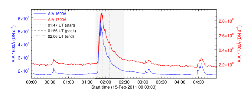
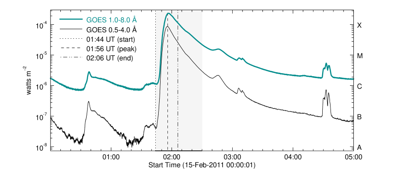
Fig. 1: Top: Light curves of the UV continuum emission from AIA 1600Å (blue curve) and AIA 1700Å (red curve), integrated over the 300″$\times$198″ subset of data centered on NOAA AR 11158. Bottom: Light curves observed by the GOES-15 satellite channels 0.5-4Å (black curve) and 1-8Å (green curve). The vertical lines mark the flare start, peak, and end times as determined by the 1-8Å channel on GOES-15. The shaded regions indicate the time period during the flare between 1:47 and 2:30. The unshaded regions on either side indicate the pre- and post-flare time periods.

The emission from both AIA channels peaked just before 01:53 UT (AIA 1600Å peaked at 01:52:41.12, and AIA 1700Å peaked at 01:52:55.71), $\sim$3 minutes before the GOES emission peaked at 01:56 UT. Both AIA UV light curves show a slight increase near the GOES end time at 02:06 UT, followed by several additional increases during the decay phase of the X-flare. The standard data reduction routine aia_prep.pro from SolarSoft (Freeland & Handy, 1998) was applied to the data from both instruments to co-align the full disk images over all channels, de-rotate them, and set a common plate scale of 0.6″ per pixel. A 300″$\times$198″ subset of data centered on AR 11158 was extracted from the full-disk set of images. To correct for solar rotation, the images were co-aligned to a common reference image by cross correlation, providing sub-pixel accuracies (McAteer et al., 2003, 2004). While several images were missing, the gaps were accounted for by averaging the two adjacent images.

Both AIA channels saturated ($\geq\!15000$ counts) in the center of the AR during the flare peak, resulting in pixel bleeding in the north and south directions during the peak of the X-class flare. A few pixels also saturated during smaller, surrounding events. These pixels were all contained within the 300″$\times$198″ subset of data throughout the duration of the time series. Where saturation occurs in the power maps, the pixel value is set to zero.

Pre-flare images of AR 11158 are shown in Figure 2. The HMI magnetograms show the magnetic configuration of the quadrupole created by two sunspot pairs. The northern pair will be designated as AR_1, where the leading positive spot is AR_1p and the trailing negative spot is AR_1n. Similarly, the southern pair will be designated as AR_2, where the leading positive spot is AR_2p and the trailing negative spot is AR_2n. Of the four events prior to and following the X-class flare, all but one occurred in AR_2n.

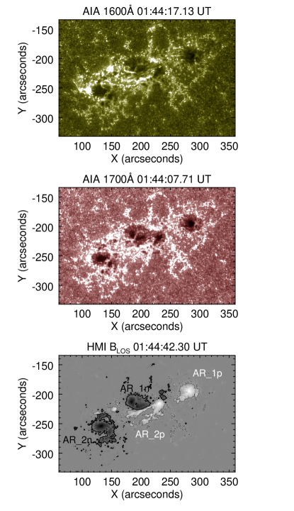
Fig. 2: AR 11158 in AIA 1600Å (top), AIA 1700Å (middle), and HMI LOS magnetogram (bottom) on 2011 February 15. The thin and thick contours outline positive (+300 Gauss) and negative (-300 Gauss) polarities, respectively. The two sunspots in the northern pair are labeled AR_1p (leading sunspot) and AR_1n (trailing sunspot). The two sunspots in the southern pair are labeled AR_2p (leading sunspot) and AR_2n (trailing sunspot).

3 Analysis

To study the spacial and temporal variations in 3-minute oscillatory power, a technique similar to that presented by Jackiewicz & Balasubramaniam (2013) and applied by Monsue et al. (2016) is employed. The method is essentially a windowed Fourier transform (WFT). Start with a data cube $f(x,y,t)$ consisting of $N$ intensity images separated by timestep $dt$ (= instrumental cadence), and spans a total duration = $N*dt$. A subset of window length $T$ is extracted, covering the time between $t_{i}$ and $t_{i}+T$, A Fast Fourier Transform (FFT) is applied to every pixel $(x,y)$ in this subset in the temporal direction. The 3-minute power at that pixel is approximated from the Fourier power spectrum by averaging the power over a frequency bin of width $\Delta{\nu}$ centered on the frequency of interest. The process is repeated for all $i=0:(N*dt)-T$, where each $i$ increment shifts the time window by one timestep $dt$. The result is an array of power maps $P(x,y,t)$.

For this study, the window length $T$ was set to 64 images ($\sim$25.6 minutes), and the frequency bin $\Delta\nu$ was set to 1 mHz centered on $\nu\sim 5.6$ mHz. Since power maps were computed starting at every possible value of $i$, there is some overlap in the time periods from which adjacent maps were obtained. This window length is necessary to achieve a frequency resolution $\delta\nu$ that allows at least two frequencies to fall within the frequency bin $\Delta\nu$ in the power spectrum. Averaging over more than one frequency point helps reduce the noise in the resulting power maps, at the expense of resolution of the flare. Two frequency points were obtained within $\Delta\nu$: at 5.21 mHz (192.00 seconds) and 5.86 mHz (170.67 seconds). The average power in the 3-minute mode was computed from these two points.

Each Fourier transform was applied without detrending the data since the frequency of interest was well outside the global flare signal. This was confirmed by applying a Fourier filter with a cutoff period longer than 400 seconds. The power spectra for the periods of interest was not altered. If a saturated pixel was encountered during the FFT computation, the value of that pixel was set to zero in the power map for that window.

4 Results and Discussion

4.1 Spatial distribution of 3-minute power

Figures 3, 4, and 5 show intensity images and corresponding spatial distribution of the 3-minute power in AIA 1600Å and AIA 1700Å before, during, and after the flare, respectively.

Throughout the 5-hour time series, enhanced 3-minute power (spatially, pixels with higher 3-minute power than others) is located over the interior or boundaries of the umbral/penumbral regions of AR 11158. Very little enhancement is observed in the quiet chromosphere (examination of the isolated power maps outside the AR confirmed that this observation was not the result of a visual scaling effect). Suppression of the 3-minute power appears in areas directly over the center of the umbra, with a ring-shaped pattern of enhanced power around the outer edges of the umbra, consistent with results obtained by Reznikova et al. (2012) using data from the 1600Å and 1700Å channels on SDO/AIA. The size of enhanced regions ranges between a few (4-6) pixels to $\gtrsim 10$ pixels, all smaller than the umbrae of the sunspots and consistent with the size of flare footpoints observed in the chromosphere. Locations of enhanced power in the maps often appear to be loosely correlated with locations of high intensity in the corresponding intensity images. However, enhanced power did not appear in every location of high intensity. This is most clearly visible in AIA 1600Å. The regions of enhanced 3-minute power were usually located along the boundaries of magnetic field strength at $\pm$300 Gauss, approximately over the outer penumbral boundary. The small areas of enhanced power emerge and fade at a later time from the same location, though the temporal resolution obtained does not allow the determination of precise times of either. One of the most prominent locations of enhanced power occurs before the flare at the bottom of the leading sunspot in the northern pair.

4.1.1 Pre-flare

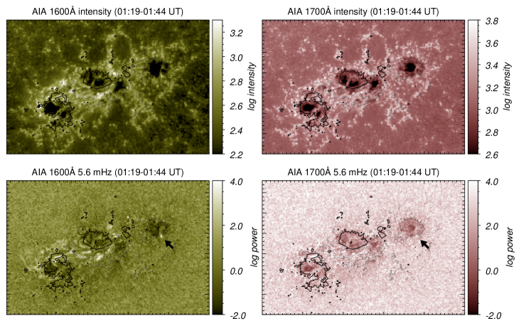
Fig. 3: Intensity and spatial distribution of 3-minute power immediately prior to the X-class flare between 01:19 and 01:44 UT on 2011 February 15, in log scale. Locations whose window included saturated pixels were set to zero. Contours indicate the approximate position of HMI B_LOS at $\pm$300 Gauss. Thin and thick contours represent positive and negative polarities, respectively. The dimensions of each image are the same as labeled on the axes in Figure 2. The arrow indicates the enhanced area discussed in the text.

Figure 3 shows intensity images and corresponding spatial distribution of the 3-minute power in AIA 1600Å and AIA 1700Å obtained from observations immediately prior to the flare (01:19-01:44). The contours represent the line-of-sight magnetic field (HMI $B_{LOS}$) at $\pm$300 Gauss. The contours indicate the approximate location of the boundary of the outer penumbra. Both the contour data and the intensity maps were obtained by averaging over the window from which the power map was computed. The alignment procedures may have resulted in a slight offset between the channels, so the position of the contours is approximate.

Locations of enhanced power are, for the most part, located along umbra/penumbra boundaries. In Figure 3, there is a bright spot with high power along the southern penumbra boundary of AR_1p, with an area of approximately 6″$\times$6″. This is indicated by the black arrow in the bottom row of Figure 3. The time series of AR intensity leading up to the X-flare reveals intermittent appearances of high intensity at this location. This enhancement in power appeared in power maps obtained from observations times as early as 40 minutes prior to flare start. Due to the length of $T$, it is difficult to resolve the temporal evolution of this region. However, since it is present in pre-flare power maps, it is possible that the power enhancement is caused by by non-thermal particles whose emission at this time was not yet strong enough for GOES flare start time.

A C-class flare occurred an hour before the X-flare, between 00:30 and 00:45 UT. The emission from the C-flare originated from AR_2n, on the opposite side of AR 11158 from the bright region discussed in the previous paragraph. Though Figure 3 does not cover this time period, it remains possible that post-flare effects from the C-flare may be present in the pre-flare data for the X-flare.

4.1.2 During the flare

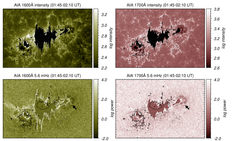
Fig. 4: Same as Figure 3, during the X-class flare between 01:45 and 02:10 UT on 2011 February 15.

Figure 4 shows intensity images and corresponding power maps obtained from observations starting at the impulsive phase, between 01:45 and 02:10 UT. Saturated pixels were excluded from the maps.

The region of enhanced power along the southern penumbral boundary of AR_1p discussed in §4.1.1 is seen in maps covering the precursor and impulsive phases of the X-flare, but does not appear in power maps obtained from the gradual phase. This may suggest this region was responding to energy input via non-thermal particles, since magnetic reconnection and particle acceleration take place during the impulsive phase.

The concentration of power enhancement in small areas located in the vicinity of sunspot umbrae suggests that these small areas of the chromosphere are responding directly to the injection of energy by a beam of non-thermal particles. Response of deeper layers in the solar atmosphere were detected via impact points localized in space in the photosphere along the outer penumbral boundary during the impulsive phase of the same flare. These sunquakes were suggested to have been triggered at the footpoints of the flux tube when it was released at the beginning of the impulsive phase (Kosovichev, 2011; Zharkov et al., 2011).

If the location of power enhancement reveals source locations of energy injection via non-thermal particle beams, then it remains possible that changes in spatial locations of these sources implies a change in the site where magnetic reconnection takes place in the corona. In fact, Kuroda et al. (2015) reported two distinct magnetic reconnection sites during the impulsive phase of the 2011 February 15 flare. Due to the saturation of pixels in AIA UV data at this time, it cannot be confirmed here whether the impulsive phase shows enhancement of oscillatory power at the same locations.

Since a large number of pixels saturated during the flare, there is little spatial information that can be extracted from power maps obtained during the flare, particularly from the AR center and parts of the outside sunspots, where emission reaches further into as the flare develops. While QPPs have been observed to persist for as many as 163 pulses during an 8-hour flare with periods between 10 and 100 seconds (Dennis et al., 2017), QPPs in flare emission often do not persist longer than three or four periods, so extracting these oscillations would be difficult even without saturation with the current methods (see review from Inglis & Nakariakov (2009)).

4.1.3 Post-flare

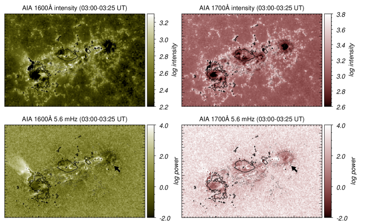
Fig. 5: Same as Figure 3, after the X-class flare between 03:00 and 03:25 UT on 2011 February 15.

Figure 5 shows intensity images and corresponding power maps obtained from observations between 03:00 and 03:25. This time window includes the first of two small events that occurred after the X-class flare. During this post-flare time period, oscillatory power enhancements are present at several small regions in the center, right around AR_2p.

4.2 Temporal evolution of 3-minute power

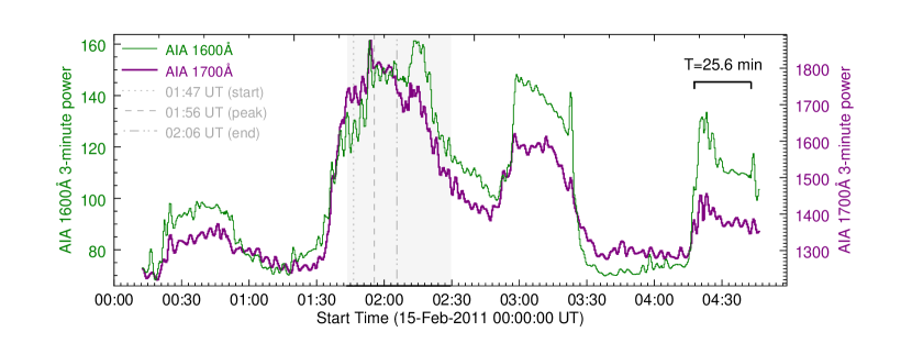
Fig. 6: Temporal evolution of the 3-minute power $P(t)$ per unsaturated pixel in AIA 1600Å (green curve) and AIA 1700Å (purple curve), obtained by summing over each 300″$\times$198″ power map. Each point in time is plotted at the center of the window over which the Fourier transform was applied to obtain the power map. The vertical dashed lines mark the GOES start, peak, and end times of the flare at 01:44, 01:56, and 02:06 UT, respectively. The shaded region covers the time period during the flare (see Figure 1 caption).

The temporal evolution of 3-minute power was estimated by reducing the 3D cube of power maps to a 1D array through time by summing each map $P_{i}(x,y,\nu)$ over $x$ and $y$ and taking the total to be the 3-minute power from the $500\times 330$ pixel subset of data centered on AR 11158. Integrating flux over the AR before applying the Fourier transform has the possible effect of reducing or canceling signal from pixels whose intensity variations are out of phase, or enhancing signal from pixels whose intensity variations are in phase. Figure 6 shows the total 3-minute power with time, obtained by shifting the array by $T/2$ so that each point is plotted at the center of the time window from which its value was obtained. The axis labelled ‘$T=25.6$ min’ is presented to illustrate the duration of the window $T$. Since each map was obtained from flux signal spanning a time window of length $T$ = 25.6 minutes, each point in the 1D array represents power from $t_{i}$ to $t_{i}+25.6$.

Since the numerical values were calculated from non-physical numbers (DN s^-1), only the relative changes and overall pattern for each channel are considered for interpretation.

After the peak in power following the peak in emission (just after GOES peak time), there is a second peak (local maximum) in the 3-minute power between $\sim$2:10 and $\sim$2:17 UT. The light curves show several peaks during the decay phase.

An increase in total emission from an AR during this phase in thermal UV wavelengths could indicate a different source of energy input. Since acceleration of non-thermal particles is no longer taking place, this could be conversion to thermal energy from another form. There may also be a change in formation height of the emission observed by each channel as flare evolves.

As observed previously by Milligan et al. (2017), the 3-minute power increases during the X-flare, as well as during the smaller events before and after, as shown in Figure 6. The persistence of the 3-minute power toward the end of the gradual phase in AIA 1700Å is consistent with the results of the wavelet analysis carried out by Milligan et al. (2017).

The amplitude of the small-scale variations in 3-minute power is higher for AIA 1700Å almost everywhere with the exception of the main phase of the X-class flare. The power from AIA 1700 is higher than AIA 1600 by 1000 counts at all points throughout the time series. Compared to 1700Å, the 1600Å 3-minute power appears to increase more (relative to its own minimum) and at a faster rate. The standard deviation for $P(t)$ from integrated flux for 1600Å is $4.9\times 10^{4}$, and for 1700Å is $2.7\times 10^{4}$.

If the emission from AIA 1600Å originates from a higher location in the atmosphere than the 1700Å emission, a possible explanation for the higher, sharper increase is that the energy from the non-thermal particle beam dissipates as it travels through deeper layers of the chromosphere. Although the emission from AIA 1700Å is generally thought to originate in lower formation heights than emission from 1600Å, the latter spans a broader temperature range, and contains emission from the C IV line. Determination of the AIA 1600Å formation height is more complicated during flares because the C IV is more likely to be contributing to the signal, and both channels may be sampling at deeper layers than they are thought to during non-flaring times.

Simões et al. (2019) investigated the spectral contribution of these two channels during flares, using high-resolution spectra from Skylab to provide reference spectra from plage observations during quiescent times. They found that flare excess emission is chromospheric in origin, and is dominated by contribution from spectral lines, while the quiet chromosphere is dominated by continuum emission.

Due to the relatively long window contributing to the power at each point in time for Figure 6, the time-resolution is rather poor, making it difficult to determine the precise flare phase during which power changed.

4.3 Time-frequency power plots

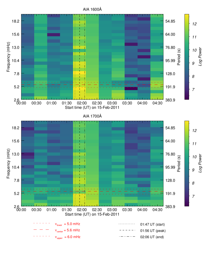
Fig. 7: Time-frequency power plots from AIA 1600Å (top panel) and AIA 1700Å (bottom panel), obtained by applying a Fourier transform to integrated emission over the 300″$\times$198″ subset of data centered on NOAA AR 11158 in discrete time increments of 64 frames ($\sim$25.6 minutes) each with no overlap (i.e. for start time $t_{0}$, then $t_{1}=t_{0}+T$, etc.). The dashed horizontal line marks the central frequency $\nu_{c}$ at $\sim$5.6 mHz, corresponding to a period of 3 minutes. The dotted horizontal lines on either side of $\nu_{c}$ mark the edges of the frequency bandpass $\Delta\nu$ = 1 mHz. The vertical lines mark the flare start, peak, and end times as determined by GOES. The power is scaled logarithmically and over the same range in both channels. Note that unlike Figure 6, the emission was summed over all pixels in the $x$ and $y$ dimensions prior to applying the Fourier transform, resulting in power values much higher than the range displayed for Figure 6, as power scales as the square of the input signal.

In addition, the resulting power is significantly lower when the Fourier transform is applied to each pixel before summing over all $x$ and $y$ in the subset, as power scales as the square of the input signal. The following section contains results computed by first integrating the flux and the power is significantly higher, as seen in Figure 7.

The technique described in §3 was applied to the integrated flux from AR 11158 over the 300″$\times$198″ subset used to compute the power maps in Figures 3, 4 and 5 and generate the plot of 3-minute power with time, shown in Figure 6. Instead of advancing in intervals equal to the instrumental cadence, the technique was applied at discrete intervals of $T=64$ images ($\sim$25.6 minutes) with no overlap (i.e. for start time $t_{0}$, then $t_{1}=t_{0}+T$, etc.) This technique is similar to one employed by Monsue et al. (2016) during two flares, here applied to an extended observation time of the flare studied by Milligan et al. (2017). It provides a way to compare the spectral power at a range of frequencies. The results are similar to those obtained with wavelet analysis, with power at a range of frequencies, each shown as a function of time, but with lower frequency and time resolution. The results are are shown in Figure 7 for frequencies between 2.5 and 20.0 mHz (400 and 50 seconds, respectively). The central frequency $\nu_{c}=5.56$ mHz and the frequency bandpass $\Delta\nu=1$ mHz between 5 and 6 mHz are marked by the horizontal dashed lines.

At all points in time when power enhancement occurs for any frequency, there appears to be a correlation with flux increase, as illustrated in the light curves in Figure 1, namely during the following time ranges: 00:30-00:45, 01:45-02:30, 03:00-03:15, and 04:20-04:45 UT. The power at all frequencies is enhanced in these plots during the X-flare compared to their non-flaring power before and after. This implies that the chromospheric plasma oscillates at a range of frequencies in response to energy injection. During the small events before and after the flare, the power at lower frequencies is enhanced, but the power at higher frequencies is suppressed relative to the same frequencies for adjacent windows.

5 Conclusions

We have presented the spatial distribution of the 3-minute oscillations associated with the X-class flare that occurred in AR 11158 on 2011 February 15. Key points are as follows:

1. Concentrated regions of 3-minute power indicate that the chromospheric plasma does not oscillate as one body.

2. The locations of increased 3-minute power during the flare are co-spatial with those of HXR flare emission, concentrated in areas $\sim$10 pixels ($\sim 4\arcsec$) across. This suggests that these small areas are manifestations of the chromosphere responding to injection of energy by nonthermal particles, and supports the theory that the chromosphere oscillates at the acoustic cutoff frequency in response to a disturbance.

3. Variation in enhancement location throughout flare phases indicates a possible change in reconnection site location from which particles are accelerated.

The temporal behavior of oscillations during the main flare remains inconclusive due to the necessary balance between temporal and frequency resolution. Techniques to improve temporal resolution, such as the standard wavelet analysis presented by Torrence & Compo (1998), will be used in future analysis to analyze additional flares (including pre- and post-flare phases) to allow the study of chromospheric behavior on timescales comparable to those over which flare dynamics are known to occur. Future work will include multiple flares smaller than X-class to reduce the number of pixels contaminated by saturation and obtain more conclusive results from the flare core region. Since the pre-flare data shown in this work includes a C-flare, it may be worthwhile to obtain more data at earlier times. Hinode/SOT observed the 2011 February 15 X-flare without saturation (Kerr & Fletcher, 2014); these data will be considered for future analysis of this flare.

References

- Beckers & Tallant (1969) Beckers, J. M., & Tallant, P. E. 1969, Sol. Phys., 7, 351, doi: 10.1007/BF00146140
- Brosius & Daw (2015) Brosius, J. W., & Daw, A. N. 2015, ApJ, 810, 45, doi: 10.1088/0004-637X/810/1/45
- Chae & Goode (2015) Chae, J., & Goode, P. R. 2015, ApJ, 808, 118, doi: 10.1088/0004-637X/808/2/118
- De Pontieu et al. (2014) De Pontieu, B., Title, A. M., Lemen, J. R., et al. 2014, Sol. Phys., 289, 2733, doi: 10.1007/s11207-014-0485-y
- Dennis et al. (2017) Dennis, B. R., Tolbert, A. K., Inglis, A., et al. 2017, ApJ, 836, 84, doi: 10.3847/1538-4357/836/1/84
- Fleck & Schmitz (1991) Fleck, B., & Schmitz, F. 1991, A&A, 250, 235
- Freeland & Handy (1998) Freeland, S. L., & Handy, B. N. 1998, Sol. Phys., 182, 497, doi: 10.1023/A:1005038224881
- Hayes et al. (2016) Hayes, L. A., Gallagher, P. T., Dennis, B. R., et al. 2016, ApJ, 827, L30, doi: 10.3847/2041-8205/827/2/L30
- Hudson (2007) Hudson, H. S. 2007, in Astronomical Society of the Pacific Conference Series, Vol. 368, The Physics of Chromospheric Plasmas, ed. P. Heinzel, I. Dorotovič, & R. J. Rutten, Heinzel
- Hudson & Fletcher (2009) Hudson, H. S., & Fletcher, L. 2009, Earth, Planets, and Space, 61, 577, doi: 10.1186/BF03352926
- Inglis et al. (2015) Inglis, A. R., Ireland, J., & Dominique, M. 2015, ApJ, 798, 108, doi: 10.1088/0004-637X/798/2/108
- Inglis & Nakariakov (2009) Inglis, A. R., & Nakariakov, V. M. 2009, A&A, 493, 259, doi: 10.1051/0004-6361:200810473
- Jackiewicz & Balasubramaniam (2013) Jackiewicz, J., & Balasubramaniam, K. S. 2013, ApJ, 765, 15, doi: 10.1088/0004-637X/765/1/15
- Kerr & Fletcher (2014) Kerr, G. S., & Fletcher, L. 2014, ApJ, 783, 98, doi: 10.1088/0004-637X/783/2/98
- Kosovichev (2011) Kosovichev, A. G. 2011, ApJ, 734, L15, doi: 10.1088/2041-8205/734/1/L15
- Kosovichev & Sekii (2007) Kosovichev, A. G., & Sekii, T. 2007, ApJ, 670, L147, doi: 10.1086/524298
- Kumar & Ravindra (2006) Kumar, B., & Ravindra, B. 2006, Journal of Astrophysics and Astronomy, 27, 425, doi: 10.1007/BF02709368
- Kuroda et al. (2015) Kuroda, N., Wang, H., & Gary, D. E. 2015, ApJ, 807, 124, doi: 10.1088/0004-637X/807/2/124
- Kwak et al. (2016) Kwak, H., Chae, J., Song, D., et al. 2016, ApJ, 821, L30, doi: 10.3847/2041-8205/821/2/L30
- Lemen et al. (2012) Lemen, J. R., Title, A. M., Akin, D. J., et al. 2012, Sol. Phys., 275, 17, doi: 10.1007/s11207-011-9776-8
- McAteer et al. (2004) McAteer, R. T. J., Gallagher, P. T., Bloomfield, D. S., et al. 2004, ApJ, 602, 436, doi: 10.1086/380835
- McAteer et al. (2003) McAteer, R. T. J., Gallagher, P. T., Williams, D. R., et al. 2003, ApJ, 587, 806, doi: 10.1086/368304
- Milligan et al. (2017) Milligan, R. O., Fleck, B., Ireland, J., Fletcher, L., & Dennis, B. R. 2017, ApJ, 848, L8, doi: 10.3847/2041-8213/aa8f3a
- Monsue et al. (2016) Monsue, T., Hill, F., & Stassun, K. G. 2016, AJ, 152, 81, doi: 10.3847/0004-6256/152/4/81
- Nakariakov & Melnikov (2009) Nakariakov, V. M., & Melnikov, V. F. 2009, Space Sci. Rev., 149, 119, doi: 10.1007/s11214-009-9536-3
- Orrall (1966) Orrall, F. Q. 1966, ApJ, 143, 917, doi: 10.1086/148567
- O’Shea et al. (2002) O’Shea, E., Muglach, K., & Fleck, B. 2002, A&A, 387, 642, doi: 10.1051/0004-6361:20020375
- Pesnell et al. (2012) Pesnell, W. D., Thompson, B. J., & Chamberlin, P. C. 2012, Sol. Phys., 275, 3, doi: 10.1007/s11207-011-9841-3
- Reznikova et al. (2012) Reznikova, V. E., Shibasaki, K., Sych, R. A., & Nakariakov, V. M. 2012, ApJ, 746, 119, doi: 10.1088/0004-637X/746/2/119
- Scherrer et al. (2012) Scherrer, P. H., Schou, J., Bush, R. I., et al. 2012, Sol. Phys., 275, 207, doi: 10.1007/s11207-011-9834-2
- Schou et al. (2012) Schou, J., Scherrer, P. H., Bush, R. I., et al. 2012, Sol. Phys., 275, 229, doi: 10.1007/s11207-011-9842-2
- Schrijver et al. (2011) Schrijver, C. J., Aulanier, G., Title, A. M., Pariat, E., & Delannée, C. 2011, ApJ, 738, 167, doi: 10.1088/0004-637X/738/2/167
- Simões et al. (2019) Simões, P. J. A., Reid, H. A. S., Milligan, R. O., & Fletcher, L. 2019, ApJ, 870, 114, doi: 10.3847/1538-4357/aaf28d
- Sutmann et al. (1998) Sutmann, G., Musielak, Z. E., & Ulmschneider, P. 1998, A&A, 340, 556
- Sutmann & Ulmschneider (1995a) Sutmann, G., & Ulmschneider, P. 1995a, A&A, 294, 232
- Sutmann & Ulmschneider (1995b) —. 1995b, A&A, 294, 241
- Tian et al. (2014) Tian, H., DeLuca, E., Reeves, K. K., et al. 2014, ApJ, 786, 137, doi: 10.1088/0004-637X/786/2/137
- Torrence & Compo (1998) Torrence, C., & Compo, G. P. 1998, Bulletin of the American Meteorological Society, 79, 61
- Van Doorsselaere et al. (2016) Van Doorsselaere, T., Kupriyanova, E. G., & Yuan, D. 2016, Sol. Phys., 291, 3143, doi: 10.1007/s11207-016-0977-z
- Viereck et al. (2007) Viereck, R., Hanser, F., Wise, J., et al. 2007, in Proc. SPIE, Vol. 6689, Solar Physics and Space Weather Instrumentation II, 66890K
- Wittmann (1969) Wittmann, A. 1969, Sol. Phys., 7, 366, doi: 10.1007/BF00146141
- Zharkov et al. (2011) Zharkov, S., Green, L. M., Matthews, S. A., & Zharkova, V. V. 2011, ApJ, 741, L35, doi: 10.1088/2041-8205/741/2/L35