The Swan: Data-driven inference of stellar surface gravities for cool stars from photometric light curves

Abstract

Stellar light curves are well known to encode physical stellar properties. Precise, automated and computationally inexpensive methods to derive physical parameters from light curves are needed to cope with the large influx of these data from space-based missions such as Kepler and TESS. Here we present a new methodology which we call The Swan, a fast, generalizable and effective approach for deriving stellar surface gravity ($\log g$) for main sequence, subgiant and red giant stars from Kepler light curves using local linear regression on the full frequency content of Kepler long cadence power spectra. With this inexpensive data-driven approach, we recover $\log g$ to a precision of $\sim$0.02 dex for 13,822 stars with seismic $\log g$ values between 0.2-4.4 dex, and $\sim$0.11 dex for 4,646 stars with Gaia derived $\log g$ values between 2.3-4.6 dex. We further develop a signal-to-noise metric and find that granulation is difficult to detect in many cool main sequence stars ($T_{\text{eff}}$ $\lesssim$ 5500 K), in particular K dwarfs. By combining our $\log g$ measurements with Gaia radii, we derive empirical masses for 4,646 subgiant and main sequence stars with a median precision of $\sim$7%. Finally, we demonstrate that our method can be used to recover $\log g$ to a similar mean absolute deviation precision for TESS-baseline of 27 days. Our methodology can be readily applied to photometric time-series observations to infer stellar surface gravities to high precision across evolutionary states.

1 Introduction

Over the last decade, there has been a substantial increase in photometric time-series observations from ground-based and space-based telescopes. With past and existing missions like CoRoT (Baglin et al., 2006; De Ridder et al., 2009), Kepler (Borucki et al., 2010; Koch et al., 2010), TESS (Ricker et al., 2014), and the upcoming PLATO (Rauer et al., 2014), we now have time-series data available for hundreds of thousands of stars. Such an abundance of time-domain data provides valuable insight about stellar physics and interiors, and advances our knowledge of stellar properties and distribution in the galaxy. Furthermore, understanding properties of host stars has important implications for exoplanet studies (Johnson et al., 2010; Huber et al., 2013; Fulton & Petigura, 2018).

One of the most successful methods to determine stellar properties from time-series data is asteroseismology, the study of stellar oscillations (Brown & Gilliland, 1994; Aerts et al., 2010; Chaplin & Miglio, 2013; Hekker & Christensen-Dalsgaard, 2017). Using high-cadence photometry, two characteristic observables can be measured from the power spectrum: the frequency of maximum oscillation power, $\nu_{\text{max}}$, and large frequency separation between two modes of the same spherical degree, $\Delta\nu$ (Brown et al., 1991; Belkacem et al., 2011; Ulrich, 1986). These two quantities allow us to calculate stellar masses and radii through scaling relations (Kjeldsen & Bedding, 1995; Stello et al., 2009; Kallinger et al., 2010; Huber et al., 2011; Casagrande et al., 2014; Mathur et al., 2016; Anders et al., 2017). For instance, Kallinger et al. (2010) used $\sim$137 days of Kepler data to derive asteroseismic mass and radius for red giants to within 7% and 3%, respectively; Silva Aguirre et al. (2017) used individual oscillation frequencies to determine mass, radius and age for 66 main sequence stars in the Kepler sample to an average precision of $\sim$4%, $\sim$2% and $\sim$10%, respectively; Huber et al. (2013) used asteroseismology to determine fundamental properties of 66 Kepler planet-candidate host stars, with uncertainties of $\sim$3% in radius and $\sim$7% in mass.

Oscillation amplitudes increase with stellar luminosity, thus making it easier to measure oscillatons in red giants (Kjeldsen & Bedding, 1995; Huber et al., 2011). However, using similar methods to calculate mass, radius and age for dwarfs becomes difficult due to their low luminosity. Moreover, oscillations in dwarfs occur at higher frequencies which cannot be detected in long cadence Kepler data. Short cadence data, while extremely useful for dwarfs, are available for only a small number of stars. Therefore, a sample of asteroseismic parameters for dwarfs is severely limited.

Alternatively, we can use granulation to derive stellar properties. The granulation signal – often referred to as the “noise” term or “background” in the power spectrum – is caused by convection on the stellar surface. Granulation signal correlates strongly with stellar surface gravity ($\log g$), and can be used to calculate $\log g$ from asteroseismic signals (Mathur et al., 2011; Kjeldsen & Bedding, 2011). This method was used to determine fundamental parameters of dwarfs in Bastien et al. (2013), but was limited by RMS measurements in the time-domain at a fixed frequency. Kallinger et al. (2016) further developed the technique to estimate $\log g$ from the auto-correlation function (ACF), but their analysis was limited to short cadence Kepler data of main sequence stars. Pande et al. (2018) transitioned to frequency space to calculate $\log g$ from the granulation signal, but used a limited region of the power spectrum in their method. Bugnet et al. (2018) also estimated surface gravities from global power in the spectrum using a random forest regressor, but with a small bias for higher luminosity and main sequence stars. While largely successful, most current methods that use granulation to extract fundamental stellar parameters do not use the full information contained in the power spectrum, are limited to certain evolutionary states, or do not quantify whether granulation has been detected.

Recent work in data-driven modelling techniques, such as The Cannon, has improved the accuracy and efficiency to which we derive stellar parameters from large astronomical data sets. The Cannon is a data-driven approach which initially has been developed to infer $\log g$, mass, effective temperature ($T_{\text{eff}}$) and chemical abundances from spectroscopic data (Ho et al., 2017b, a; Casey et al., 2016, 2017; Wheeler et al., 2020; Sit & Ness, 2020; Rice & Brewer, 2020). Ness et al. (2018) presented the first application of The Cannon on Kepler time-series data, and modeled the auto-correlation function to recover $\log g$ to a precision of $<0.1$ dex. However, their analysis was applied to red giants only.

In this paper, we expand on the work by Ness et al. (2018) to estimate $\log g$ from the power spectrum of main sequence, subgiant and red giant stars using long cadence Kepler data. We develop a new method which we call The Swan , which employs local linear regression to infer $\log g$ using a localised training set around each star under consideration, and derive stellar masses using radii from Gaia. We compare the success of previous data-driven methods like The Cannon to our model, and investigate the effect of photometry baseline on $\log g$ inference.

2 Observations

2.1 Target Selection

To use data-driven inference techniques, we create a reference set of main sequence, subgiant and red giant stars for which $\log g$ is well known and granulation can be detected. We select 16,947 stars with asteroseismically derived stellar surface gravities in Mathur et al. (2017), who compiled seismically derived stellar parameters from various catalogs (Bruntt et al., 2012; Thygesen et al., 2012; Stello et al., 2013; Chaplin et al., 2014; Huber et al., 2011, 2013, 2014; Pinsonneault et al., 2014; Casagrande et al., 2014; Silva Aguirre et al., 2015; Mathur et al., 2016), and 16,094 stars with seismically derived masses, radii, and surface gravities in Yu et al. (2018). By cross-referencing both catalogs, we select 19,273 stars with asteroseismic surface gravities. This sample is hereafter referred to as the seismic sample.

Furthermore, low frequency stellar variability that is not due to granulation can mask the granulation signal that we want to measure. To measure only the granulation background, we removed any rotating stars (McQuillan et al., 2013), classical pulsators (Debosscher et al., 2011; Murphy et al., 2019), eclipsing binaries (Abdul-Masih et al., 2016) and Kepler exoplanet host stars (Thompson et al., 2018). In total, we removed 1,851 stars exhibiting non-granulation like variability from the seismic sample. To ensure we use the most recent stellar parameters, we removed 998 stars not found in Berger et al. (2018), 216 stars with photometry less than 89 days and 1,788 stars for which we could not find Quarter 7-11 data. We also removed 252 stars that performed below a 50% duty cycle (see Section 2.2). The final seismic sample contains 14,168 stars.

In the top panel of Figure 1, we plot the distribution of stars in the seismic sample on a Hertzsprung-Russell (H-R) diagram. Stellar $\log g$ values for this sample are calculated using asteroseismic scaling relations. This sample contains mostly giants due to their high signal-to-noise ratio which makes it possible to measure global seismic observables, such as $\nu_{\text{max}}$ and $\Delta\nu$, to derive stellar properties.

To expand the sample of dwarfs and subgiants, we chose stars for which granulation has been successfully detected by Pande et al. (2018), hereafter referred to as the Gaia sample. The catalog contains 15,109 stars, but 6,736 stars overlap with the seismic sample. Because stellar parameters measured from asteroseismology are more accurate and precise, we classified overlapping stars as an asteroseismic measurement due to their high precision. Out of the remaining 8,373 stars, we removed 1,834 stars that exhibit other types of variability. We further removed 392 stars not found in Berger et al. (2018) to ensure we use recently derived stellar parameters. Out of the remaining 6,147 stars, we removed 84 stars with photometry less than 89 days, 88 stars performing below a 50% duty cycle (see Section 2.2), 10 stars for which we could not retrieve Quarter 7-11 data, and 2 stars for which there was no $\log g$ value available in Berger et al. (2020). The final Gaia sample contains 5,964 stars.

The bottom panel of Figure 1 shows the distribution of stars in the Gaia sample. Compared to the seismic sample, the Gaia sample contains many more dwarfs since it does not suffer from the seismic detection bias (Chaplin et al., 2011). The $\log g$ values for this sample are calculated from isochrone fitting in Berger et al. (2020) who used recent MESA Isochrones and Stellar Tracks (MIST) models (Choi et al., 2016; Dotter, 2016; Paxton et al., 2011, 2013, 2015), SDSS g and 2MASS $K_{s}$ photometry, Gaia DR2 parallaxes, red giant evolutionary state flags and spectroscopic metallicities to derive a homogeneous set of stellar parameters. Median fractional uncertainties for derived stellar surface gravity are on the order of 0.05 dex, with $\log g$ distribution peaking at 4.24 dex.

In this work, giants are defined as stars with a $\log g$ below 3.5 dex, while dwarfs and subgiants have a $\log g$ above or equal to 3.5 dex. We obtained $\log g$ values for most dwarfs from Berger et al. (2020), and $\log g$ values for subgiants and giants from Mathur et al. (2017) and Yu et al. (2018). If a star was available in all three catalogs, asteroseismic measurements were prioritized. If the $\log g$ was unavailable in the seismic catalogs, the label was obtained from Berger et al. (2020). Our final reference sample contains 20,132 stars exhibiting granulation with $\log g$ measurements from asteroseismology (Mathur et al., 2017; Yu et al., 2018) and isochrone fitting (Berger et al., 2020).

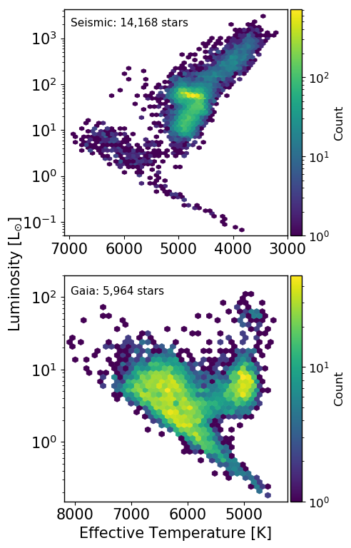
Figure 1: Hertzprung-Russell (H-R) diagrams of stars in our reference sample. Top: Luminosity versus effective temperature for 14,168 in the seismic sample. Bottom: Luminosity versus effective temperature for 5,964 stars in the Gaia sample. Colour-coding represents number density.

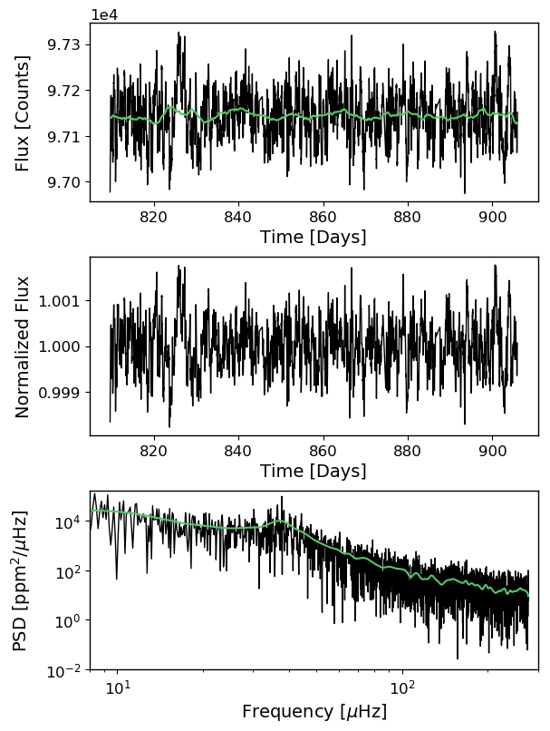
Figure 2: Overview of steps taken to prepare the data. Top: Raw Kepler long cadence light curve of Kepler ID 8812919. Black curve is the outlier corrected light curve and the green line is the smoothed light curve using a width of $\sim$8 days. Middle: Normalized flux after removing long-periodic (low-frequency) variations. Bottom: Power spectrum of normalized light curve in black. The green line represents the power spectrum smoothed by 2 $\mu$Hz and effectively traces the granulation signal of the star.

Table 1: White noise level as a function of Kepler magnitude calculated using 3,270 Kepler stars observed in short cadence.

Kepler Magnitude	White Noise Level [ppm${}^{2}/\mu$Hz]
8.0	0.17
8.1	0.19
8.2	0.21
…	…
15.8	963.30
15.9	1109.85
16.0	1278.83

Note. — The full table in machine-readable format can be found online.

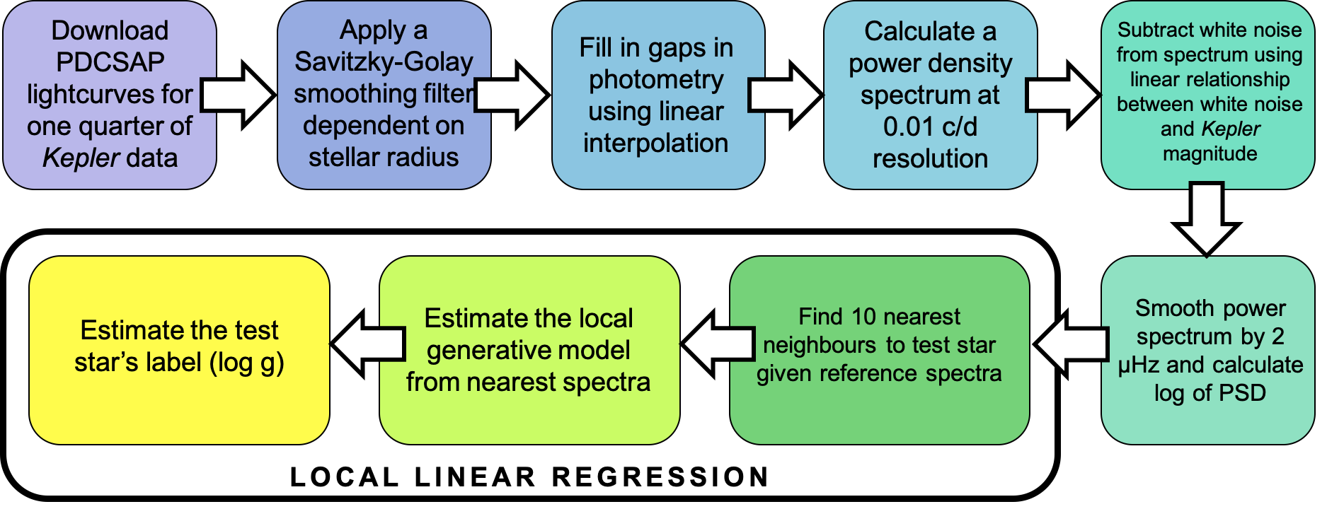
Figure 3: Overview of The Swan pipeline including details on the preparation of input data and application of local linear regression as described in Sections 2 and 3.1.

2.2 Data Preparation

To predict stellar surface gravity from power spectra, we prepared long cadence Kepler data (29.4 minute sampling) to train and test our model. We use a single quarter of Kepler data, or $\sim$90 days, to minimize data-processing and validate our model on the shortest available photometry baseline. Figure 2 shows the steps we followed for data preparation as described below:

1. We downloaded Pre-Search Data Conditioning Simple Aperture Photometry (PDCSAP) from MAST for stars with Quarter 9 data. We only selected stars for which we had Gaia stellar parameters as found in Berger et al. (2018). For stars without Quarter 9 data, we tried to find data in adjacent quarters and removed any stars from our sample for which there was no Quarter 7-11 data available. For the seismic sample, the number of stars in Quarter 9-11 were 10,104, 3,808 and 256, respectively. For the Gaia sample, the number of stars in Quarter 9-11 were 5,622, 338 and 4, respectively.

2. We only kept data points with good quality flags (flags = 0).

3. We removed any stars that had a duty-cycle less than 50%.

4. We performed a running sigma-clipping routine with 50 data points in each subset and removed outliers greater than 3$\sigma$.

5. We applied a smoothing Savitzky-Golay filter to remove any long-periodic (low-frequency variations). To create a relation between smoothing filter and stellar radius, we used the radius and $\nu_{\text{max}}$ measurements for stars in Yu et al. (2018), along with the empirically derived smoothing function d=0.61+0.04$\nu_{\text{max}}$ as mentioned in Yu et al. (2018). The smoothing width for each star varied according to the following relation given a stellar radius in solar units:

   $$d\;[\mu\textrm{Hz}]=0.92+23.03\;e^{-0.27\;\textrm{R}/\textrm{R}_{\odot}}$$ (1)

   The filters ranged from 0.5 - 12.6 days, where a filter of $\sim$12.6 days was applied to stars with stellar radius above $\sim$30 R_⊙.

6. Any remaining gaps in the data created by bad quality flags were filled in using linear interpolation to avoid leakage of power towards higher frequencies in the power spectrum (García et al., 2014; Pires et al., 2015). We followed the interpolation by removing any remaining data points in the smoothed and normalized light curve greater than 5$\sigma$ from the flux median.

7. We calculated a power density spectrum with a frequency spacing of $\sim$0.12 $\mu$Hz (or $\sim$0.01 c/d) corresponding to a critically sampled spectrum.

8. We subtracted the contribution from white noise using a linear relationship between Kepler magnitude (Kp) and white noise (see Table 1) where Kp values were obtained from Kepler Input Catalog (KIC, Brown et al. (2011). The relation was created using one quarter of Kepler data from 3,270 stars observed in short cadence and prepared using steps i-vii. The white noise was calculated as the average power between frequencies 6,000-8,000 $\mu$Hz. We subtracted the white noise from the unsmoothed spectrum for frequency bins with granulation power greater than the white noise. This step ensured that we recovered most of the granulation signal in the spectrum especially for faint stars.

9. We smoothed the power spectrum by 2 $\mu$Hz to remove sharp peaks in amplitude. We experimented with the smoothing value, and chose a value that ensured we did not lose information in the spectrum, that is, did not compromise the precision of our inferred labels (as parameterized by the RMS scatter and median standard deviation).

3 Local Linear Regression applied to Light Curves

3.1 The Swan

Local models (sometimes also referred to as “kernel methods”; see e.g. Hastie et al., 2009 chapter 6 for an introduction) capture a non-linear relationship between labels and data by combining linear models to the small region around each datapoint. Local Linear Models (LLM) find a natural application in large data sets where the data are a globally complex, but smooth function of labels. By “zooming in” to a regime where the model is approximately linear, local linear regression can capture globally non-linear behavior with a mathematically simple model (see, e.g. Hogg et al., 2010 for a review of linear regression). While local methods often fail in application to high dimensional data, the smoothed stellar power spectra of time-domain photometry (light curves) have few degrees of freedom (Anderson et al., 1990). For our application, the data is the noise-corrected power spectrum of the light curves and the label we infer is the $\log g$ parameter for each.

In brief, for each test object, The Swan uses training data in the local neighbourhood to infer labels via regression. Given $\mathbf{G}$, taken to be a vector of the points in the log power spectrum of a star for which we would like to obtain labels, we find the $k$ power spectra in the training set with the smallest Euclidean distances, $d$, from $\mathbf{G}$:

$$d=|\mathbf{G}-\mathbf{G}_{\text{train}}|\quad,$$ (2)

where $G_{\text{train}}$ is the Power Spectral Density (PSD) vector from the training set. We take $\Gamma$ to be the matrix whose rows are the neighboring training spectra, and $L$ to be the matrix whose rows are the label vectors of the neighbors. Since we use a single label, $L$ is a vector of the $\log g$ values for each neighboring star. We standardize $\Gamma$ and $\mathrm{G}$ by re-expressing them in coordinates such that the mean neighboring spectrum is zero, and the standard deviation of the power spectral density among the neighbors is one at each frequency. Our prediction for the label vector (or label) associated with $\mathbf{G}$ is then given by,

$$\widehat{\ell}=(L^{+}\Gamma)^{+}\mathbf{G}\quad,$$ (3)

where “⁺” denotes the Moore-Penrose pseudoinverse defined for real orthogonal matrices as

$$A^{+}=(A^{T}A)^{-1}A^{T}\quad.$$ (4)

This linear operation has a simple interpretation. $L^{+}\Gamma$ is the maximum-likelihood estimate (MLE) for the matrix that maps labels (values of $\log g$) to power spectra, assuming that the labels are known exactly and the PSD at each frequency in each power spectrum has independent equal Gaussian uncertainty. While the measurement uncertainty on each power spectrum is neither Gaussian nor homoscedastic, it is much smaller than the model prediction error, indicating that a more careful treatment would be unhelpful. $\widehat{\ell}$ is the MLE for the labels associate with $\mathbf{G}$ given $L^{+}\Gamma$; it is the label(s) that yields a predicted power spectrum closest to $\mathbf{G}$. The best-fit model spectrum (that generated exactly from $\widehat{\ell}$) is given by $\widehat{\ell}^{T}(L^{+}\Gamma)$. We tried using a discriminative linear model ($\widehat{\ell}=\mathbf{G}^{T}\Gamma^{+}L$) rather than a generative one, but found that it performed slightly worse in cross-validation.

In Figure 3, we show a schematic of The Swan, including the steps taken to prepare the data for local linear regression. To summarize, the input to The Swan is the logarithmic power spectral density and labels that describe the data. To estimate the $\log g$ from a power spectrum, The Swan finds the most similar spectra in the training set (those which minimize Equation 2). It then performs linear regression on those spectra only to infer the relationship between $\log g$ and power spectral density, and uses that generative model to estimate the $\log g$ of the spectrum at hand (Equation 3).

We experimented with the number of nearest neighbours (ie. $k$ = 5, 10, 20, 50 and 100) and found there was only a slight difference in The Swan’s performance for small $k$ compared to large $k$, and worsened for $k$ above 50. We chose $k=10$ as the number of nearest neighbours. This value of $k$ is computationally trivial, and ensures there are enough stars to model well the relationship between the power spectral density and the $\log g$ label.

3.2 Seismic sample

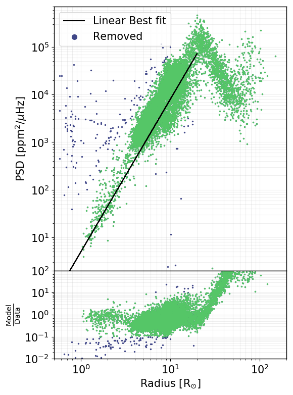
Figure 4: Mean power spectral density between 10-12 $\mu$Hz as a function of stellar radius for stars in the seismic sample. Stars dominated by variability other than granulation are identified as outliers which are shown as blue data points, while green data points represent stars that pass our test for no additional variability (and below 20 R_⊙ represent stars within 10 ppm²/$\mu$Hz of the best fit line).

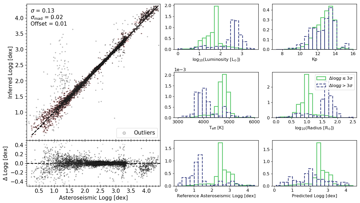
Figure 5: Left: Surface gravities for the seismic sample inferred with The Swan, compared to the asteroseismic $\log g$ reference labels. The top left hand corner shows the precision and bias metrics of the inference, where $\sigma$ is the root mean square (RMS) and $\sigma_{\textrm{mad}}$ is the robust standard deviation for 14,003 stars (including outliers). Outliers, defined as stars with a difference between their reference and inferred $\log g$ above $3\sigma=0.38$ dex, are shown in grey and errors in asteroseismic $\log g$ are shown in red. The bottom left panel shows the difference between the reference asteroseismic $\log g$ and inferred $\log g$. Right: Histograms demonstrating the properties of stars in the seismic sample. The green solid bars show normalized counts for non-outliers and the purple dashed bars show normalized counts of outliers.

To validate our model, we first applied The Swan on the seismic sample where $\log g$ is measured using asteroseismic scaling relations (Mathur et al., 2017; Yu et al., 2018). These reference $\log g$ values serve to label each test star, by building a model using its nearest neighbours in data space as described in Section 3.1. This is equivalent to cross-validation, since a test star itself is not used to estimate its own label. We can then compare the reference $\log g$ value for the test star to our inferred $\log g$ value.

In generating results of the seismic analysis, we made some additional quality cuts on the data beyond the complete reference set. While we had first removed stars from our sample that showed non-granulation like variability and also applied a high-pass filter to attenuate the rotation signal, our initial cross-correlation tests of our inferred versus reference $\log g$ label showed a number of outliers, with high amplitude at low frequencies in their power spectra. These stars correspond to fast rotators with prevalent harmonics in the spectrum. This makes them sufficiently different from the rest of the data since the linear model can not capture the power amplitude as a function of the $\log g$ label. To screen for stars with harmonics in the spectrum, we asserted a linear relationship in log-log space between the average power spectral density at low frequencies and stellar radius from Gaia, and modeled it using the following relationship:

$$\log_{10}(\text{PSD}/(\text{ppm}^{2}/\mu\text{Hz}))=3.2\log_{10}(\text{R/R}_{\odot})+0.7$$ (5)

Figure 4 shows mean power spectral density between 10-12 $\mu$Hz as a function of stellar radius. The turnoff at 20 R_⊙ corresponds to the impact on the data of applying this filter on stars with large radii. The best fit line was found by fitting the relationship between PSD and stellar radius for radii below 20 R_⊙. We removed any stars with a power spectral density larger than 10 $\text{ppm}^{2}/\mu\text{Hz}$ from the best fit line for radii below 20 R_⊙, and kept all stars above this threshold. Through this filter, we removed $\sim$1.1% of the seismic sample, or 160 from an original 14,168 stars.

Furthermore, we inspected the residual sum of squares (RSS) between the The Swan’s model and smoothed power spectrum of each star. This serves as a check of how well our model matches our data, so we can remove any poorly modeled stars. We removed any stars with RSS above 100 (ppm${}^{2}/\mu$Hz)²; this filter removed a further 5 stars, or $\sim$0.04% of the sample.

Figure 5 shows our final results for the seismic sample. We observe excellent agreement between the inferred and asteroseimic $\log g$, with a robust standard deviation ($\sigma_{\textrm{mad}}$) of 0.02 dex with no significant bias for 14,003 stars, including outliers. Figure 5 demonstrates that The Swan can successfully infer $\log g$ from stellar power spectra to high precision across five orders of magnitude in surface gravity. Inferred $\log g$ values and other stellar parameters for the seismic sample are provided in Table 3.

Only 181 out of 14,003 stars, or $\sim$1.3 % of the final sample shown in Figure 5 are classified as outliers, where we define outliers to be greater than 3$\sigma$ from the reference $\log g$ label. To investigate these 181 outliers, we plotted normalized histograms to show stellar properties of outliers compared to stars with successful inference in the right panel of Figure 5. Outliers peak at higher radii, lower effective temperatures, and lower surface gravities. This indicates that outliers in the seismic sample are evolved, high luminosity stars.

A possible reason for the presence of outliers in our inference could be that rotation modulation is mixed in with the granulation signal in the power spectrum. This would indicate that our removal of long-period variations from the light curve during initial data processing steps was not completely successful. For instance, applying a wide smoothing filter on $\sim$90-days of photometry on evolved stars has little effect on removing the long-periodic variations, while applying a narrow filter below 2 days removes the granulation signal that we want to measure. Additionally, a lack of label space coverage of the training objects within this particular parameter space could also contribute to unsuccessful inference for bright stars. For instance, only $\sim$5% of the combined seismic and Gaia samples have high radii (917 seismic stars with radii above 30 R_⊙) and $\sim$6% have high luminosities (1104 seismic stars with luminosities above 200 L_⊙). Therefore, for evolved stars or stars above 30 R_⊙, The Swan is not successful on one quarter of Kepler data, presumably due to our inability to measure granulation in the power spectrum, as well as a sparsely populated training set within this region.

3.3 Gaia sample

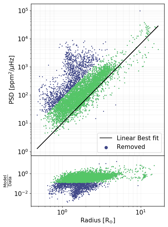
Figure 6: Mean power spectral density between 10-12 $\mu$Hz as a function of stellar radius for stars in the Gaia sample. Stars dominated by variability other than granulation are identified as outliers which are shown as blue data points, while green data points represent stars within $\sim$7.9 ppm${}^{2}/\mu$Hz of the best fit line.

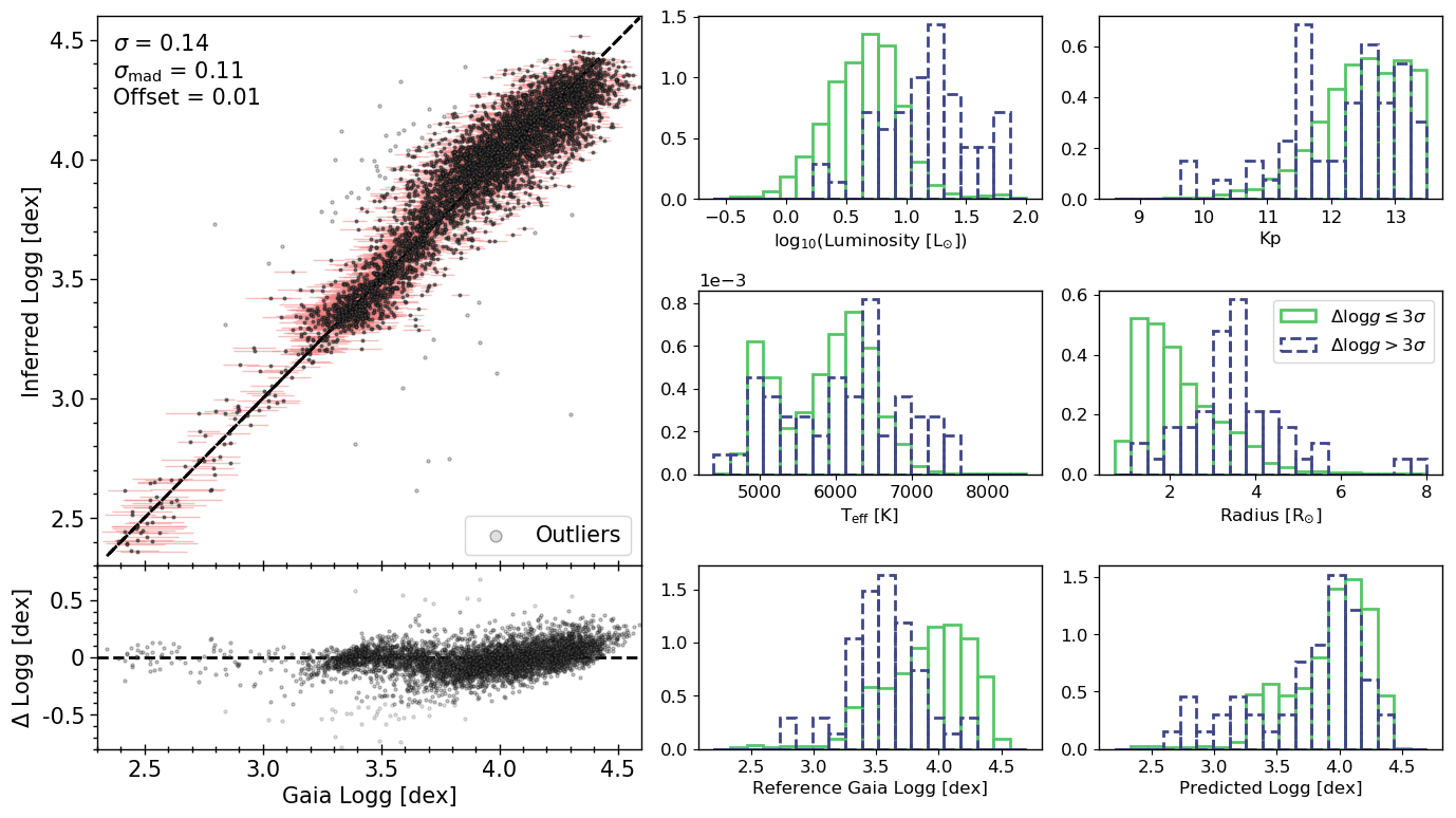
Figure 7: Left: Surface gravities for Gaia sample inferred with The Swan, compared to the reference $\log g$ values as derived in Berger et al. (2020). The bottom left panel shows the difference between the reference Gaia $\log g$ and the inferred $\log g$. The top left hand corner shows the precision and bias metrics of the inference, where $\sigma$ is the root mean square (RMS) and $\sigma_{\textrm{mad}}$ is the robust standard deviation for 4,697 stars (including outliers). Outliers, defined as stars with a difference between their reference and inferred $\log g$ above $3\sigma=0.41$ dex, are shown as grey points, and errors in Gaia $\log g$ are shown in red. Right: Histograms demonstrating stellar properties of the Gaia sample. The green solid bars show normalized counts for non-outliers, and the purple dashed bars show properties of outliers.

We performed similar analysis for the seismic sample on the Gaia sample, which contains stars with $\log g$ measured through isochrone fitting (Berger et al., 2020). Similar to the seismic sample, initial analysis of the Gaia sample showed outliers in the cross-correlation plot, corresponding to stars which have high power spectral density at low frequencies. Figure 6 shows mean power spectral density between 10-12 $\mu$Hz as a function of stellar radius for the Gaia sample. Unlike Figure 4, Figure 6 does not include the turnoff at $\sim$20 R_⊙ because the Gaia sample does not include many evolved stars. We modeled the distribution in Figure 6 using Equation 5, and removed stars with power density larger than $\sim$7.9 $\text{ppm}^{2}/\mu\text{Hz}$ from the best fit line. Through this filter, we removed $\sim$21% of the sample, or 1,258 from an original 5,964 stars. We also removed stars with residual sum of squares above 100 (ppm${}^{2}/\mu$Hz)² which removed a further 9 stars.

Figure 7 shows the comparison between the inferred $\log g$ using local linear regression and reference Gaia $\log g$ derived in Berger et al. (2020), with residuals shown in the bottom left panel. The final cross-validation gives a robust standard deviation of 0.11 dex with no significant bias for 4,697 stars, including outliers. Inferred $\log g$ values and other stellar parameters for this sample are provided in Table 4.

Figure 7 shows a fairly strong correlation but with a large scatter for stars with $\log g$ above $\sim$3.5 dex. Only 51 out of 4,697 stars, or $\sim$1% of the sample, are classified as outliers. Similar to the seismic sample, we explored the cause of outliers by plotting normalized histograms of stellar parameters representing outliers and the rest of the sample shown in the right panel of Figure 7. Outliers peak at higher luminosities, higher radii and lower surface gravities.

Some of the outliers could be due to pixel contamination, for example through an asteroseismic signal being blended into the Kepler aperture of the target stars (Hon et al., 2019). To explore this, we investigated contamination values of Kepler data from MAST, as well as the re-normalized unit-weight error (RUWE) value from Gaia (Lindegren et al., 2018). MAST provides a measure of contamination due to neighbouring stars where a value of 0 implies no contamination and a value of 1 implies light is all due to background. RUWE is the magnitude and colour-independent re-normalization of the astrometric $\chi^{2}$ fit in Gaia DR2, which is sensitive to close binaries (Gaia Collaboration et al., 2018; Evans, 2018; Lindegren et al., 2018; Berger et al., 2020). Out of the 61 outliers, only 15 stars have an RUWE above 1.2, which is a typical indicator of binarity. Out of the entire Gaia sample, 11% of stars – or 517 out of 4,697 – have a RUWE above 1.2. Additionally, none of the outliers in our sample had a MAST contamination parameter above 0.027. We conclude that contaminating flux and stellar binarity from nearby stars are not driving our misestimated $\log g$ values.

We further investigated the differences between Figures 5 and 7. The $\log g$ values in the seismic sample are calculated using scaling relations which give very precise stellar parameters (Mathur et al., 2017; Yu et al., 2018). The $\log g$ values in the Gaia sample have larger error bars and are calculated through isochrone fitting which chooses the most likely models based on input parameters and their uncertainties (Huber et al., 2017; Berger et al., 2020). For instance, Gaia parallax and 2MASS K magnitude provide a luminosity which are combined with a colour and isochrones to derive $\log g$. This produces less precise $\log g$ values ($\sim$0.05 dex versus $<$0.03 dex from asteroseismology), which may additionally be affected by systematic errors from the use of a single isochrone grid. Therefore, we believe the success of The Swan is highly dependent on the accuracy of the labels in the reference set, and that the difference in predictive uncertainty achieved for the seismic and Gaia samples is driven by the uncertainty of the training $\log g$ values.

3.4 S/N Metric for Detecting Granulation

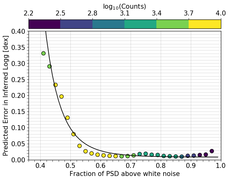
Figure 8: Predicted uncertainty in inferred $\log g$ as a function of fraction of power spectral density above white noise level. Absolute standard deviation was calculated using non-outliers in the seismic and Gaia samples for each 0.02 increment of signal-to-noise (S/N). The solid curve represents the best-fit to the data using a power law. The data points are coloured by the number of stars within the specified S/N range used to calculate predicted uncertainty.

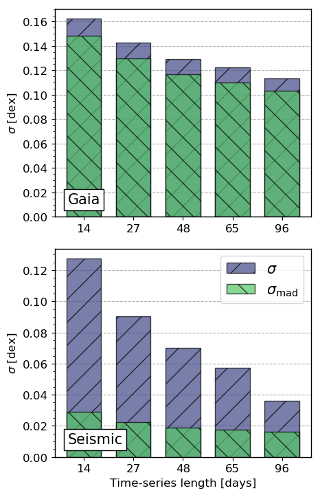
Figure 9: Recovered precision of surface gravity as a function of photometry length for the Gaia and seismic samples. The green and purple bars show the standard deviation and the robust standard deviation using median absolute deviation respectively.

To explore the source of the systematic differences in Figure 7, we calculated a signal-to-noise (S/N) metric by counting the number of points in the spectrum with power above the white noise level as a fraction of the total number of points, resulting in a S/N range of $\sim$0.02 to 1.0 for the combined seismic and Gaia samples.

To investigate the S/N value pertaining to a white noise dominated spectra, we generated over 12,000 ‘noisy’ light curves and calculated the power above the white noise in the power spectrum, where the white noise level was chosen as the average power at frequencies between 270-277 $\mu$Hz. The median S/N from simulated light curves was 0.45 indicating that we can expect S/N of $\sim$0.45 or below for white noise dominated spectra where granulation cannot be measured.

In fact, the comparison in Figure 7 improves when we apply a S/N cut to our inferred $\log g$ values for the Gaia sample. As the value of S/N cut increases, we retain less of the sample, but the bias seen at higher $\log g$ diminishes in Figure 7. This improvement due to a cut in S/N supports our conclusion that stars with low S/N are too faint to detect granulation.

Indeed, our inferred $\log g$ values are systematically lower than predicted by evolutionary models for cool main sequence stars such as K dwarfs. While small biases may be expected from systematic model errors (e.g. Boyajian et al., 2013), it is more likely that the lack of detectable granulation leads to an underestimation of $\log g$. This implies that applying granulation-based $\log g$ to K dwarfs is only possible for the brightest stars, even in the Kepler sample.

3.5 Uncertainties in Inferred $\log g$

To derive uncertainties in our inferred $\log g$ values, we applied The Swan on both the seismic and Gaia samples by adding white noise to the photometry to investigate the scatter in inference as a function of S/N. To anticipate the noise embedded in the photometry, we simulated 10,000 sets of noisy data between 0.001-$10^{4}$ ppm and produced a relationship between time domain noise and white noise in the power spectrum. The resulting relation was combined with our previously derived relation between white noise level and Kepler magnitude (see Section 2) to create a correlation between time domain noise and Kepler magnitude.

To quantify how the inference degrades for a noise dominated light curve, we applied The Swan on photometry with added noise ranging from 0.5 to 6 times the time domain noise. The noise was only added to the test star and not the entire set of reference stars, and the remaining data were prepared following steps outlined in Section 2.

We derived uncertainties in inferred $\log g$ values by combining The Swan’s results from seismic and Gaia samples with many different amplitudes of noise added. Figure 8 shows the robust standard deviation ($\sigma_{\textrm{mad}}$) in $\log g$ inference as a function of S/N between 0.1-1.0, with S/N bin width of 0.02, coloured by the number of stars within the specified S/N range. For instance, a star with S/N between 0.50-0.52 would have a typical error of 0.08 dex on its inferred $\log g$ measurement. We used the following equation to fit a relation between S/N and predicted error in inferred $\log g$ values,

$$\sigma=3.39\cdot 10^{-4}s^{-8.06}+6.75\cdot 10^{-3}$$ (6)

where $s$ is the S/N and $\sigma$ is the predicted inferred $\log g$ uncertainty in dex. Stars with S/N below 0.36 and above 0.96 were removed from the fitting routine due to small number of stars with S/N in this range. Equation 6 was used to assign errors to inferred $\log g$ measurements in Tables 3 and 4. An uncertainty floor of 0.02 dex was set for any predicted uncertainties below 0.02 dex.

In Figure 8, the scatter increases for lower S/N values implying that a lack of granulation signal makes it difficult for The Swan to make a successful inference. Therefore, we do not report a $\log g$ measurement for any stars with S/N below 0.36 due to an unsuccessful inference. Stars with S/N above 0.96 were assigned an error of 0.2 dex since most stars with S/N in this range are high-luminosity giants for which one quarter of Kepler is not sufficient to successfully measure granulation. For future use of The Swan, we recommend caution in derived $\log g$ measurements for any star with S/N below 0.45 and radius above 30 R_⊙.

3.6 Photometry Baseline

We explored the effect of photometry length on The Swan’s performance to estimate the precision achievable with data from other surveys. While Kepler delivered light curves at a baseline of roughly 90 days at 29.4 minute cadence, TESS provides time-series photometry at two cadences with a baseline ranging from 27 days to a full-year. Therefore, we tested our model on four photometry baselines of 14, 27, 48 and 65 days with no change in cadence. To process the light curve, we only selected data points if they occurred at days less than the specified baseline. Aside from truncating the light curves, we prepared the data as described in Section 2.2.

Figure 9 shows the effect of shortened photometry length on the precision of recovered $\log g$ using The Swan on the seismic and Gaia samples. As expected, the scatter increases as the length of the light curve decreases, affecting both the root mean square (RMS) and the robust standard deviation (MAD). For the Gaia sample, the RMS scatter at 27 days is $\sigma=0.14$ dex, which is 23% larger than the RMS scatter at 96 days (full length photometry). However, high precision, measured by $\sigma_{\textrm{mad}}$ = 0.11 dex, is still achieved despite the shorter baseline.

For the seismic sample, while the RMS scatter doubles at 27 days compared to full-length photometry (from $\sigma$ = 0.04 dex to 0.09 dex), the MAD precision is still less than 0.03 dex for the shorter baseline. Unlike the Gaia sample, there is a significant difference between the RMS and the robust standard deviation, where the RMS at 27 days (TESS-baseline) is over twice as large as the RMS at full-length photometry. Therefore, the use of The Swan on shorter baseline data produces more outliers. These individual objects are not the same outliers when using the longer baseline ($\sim$90 days) data. As expected, higher quality data produces higher precision results which emphasizes the importance of a high quality training set to obtain high fidelity training labels.

Nevertheless, we expect The Swan to recover stellar parameters with an increased scatter for TESS-like data (27 days) compared to full Kepler light curves. However, the shorter baseline still produces precision comparable to, or even less than, data-driven methods found in literature (Casey et al., 2016; Ness et al., 2015, 2016, 2018). Therefore, The Swan can be successfully applied to TESS photometry to infer stellar properties despite a shorter baseline.

4 A Comparison: inference of $\log g$ using The Cannon

To investigate the inference of stellar surface gravity using The Cannon (Ness et al., 2018), we use a single label second-order polynomial model that is built on our training set of data. Like The Swan, this is data driven: a reference set of stars (training set) are used to infer labels for a new set of stars (test set). However, The Cannon as implemented in Ness et al. (2018) is quite distinct from The Swan, which builds a local model using nearest neighbours in the data space for every test object that is labeled. We briefly describe The Cannon below and refer the reader to Ness et al. (2015) and Ness et al. (2018) for a more detailed discussion.

To use The Cannon on time-series data, the data must satisfy the following conditions: (a) stars with the same labels must have the same spectra and (b) power density at a given frequency should vary smoothly with stellar labels. To use The Cannon, we converted our data to the frequency domain, by taking the Fourier Transform denoted by $g(f)$. We then smoothed over the power spectrum by 2 $\mu$Hz to remove sharp peaks produced by oscillation modes in the spectrum.

We take $n$ reference objects with their known labels $\ell$. The spectral model is characterized by a coefficient vector $\theta$ that allows the prediction of the amplitude, $G_{nf}$, at every frequency $f$ of the power spectrum for a given label vector:

$$\ln p(G_{nf}|\theta^{T}_{f},\ell_{n},s^{2}_{f})= -\frac{1}{2}\frac{[G_{nf}-\theta^{T}_{f}\cdot\ell_{n}]^{2}}{s^{2}_{f}+\frac{\sigma^{2}_{nf}}{g_{nf}}}$$ (7)

$$-\frac{1}{2}\ln(s^{2}_{f}+\frac{\sigma^{2}_{nf}}{g_{nf}})$$

The noise term is a combination of uncertainty variance at each frequency and the intrinsic variance of the model of the fit, $s^{2}$. A term $1/g_{nf}$ is included to represent propagated amplitude error since the data are transformed to a logarithmic amplitude. At training time, the coefficient vector for the quadratic model is solved for at every frequency step. We solve for 3 coefficients at each frequency step, such that $\ell_{n}$=[1, $\log g$, $\log g$ ²].

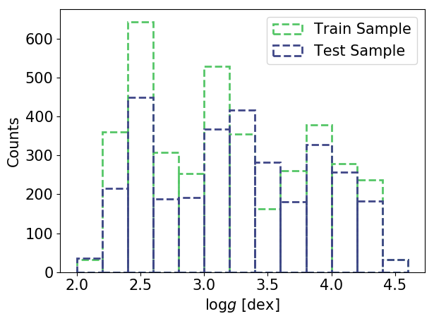
Figure 10: Distribution of stellar surface gravity ($\log g$) used for training (3,692 stars) and testing (3,675) The Cannon.

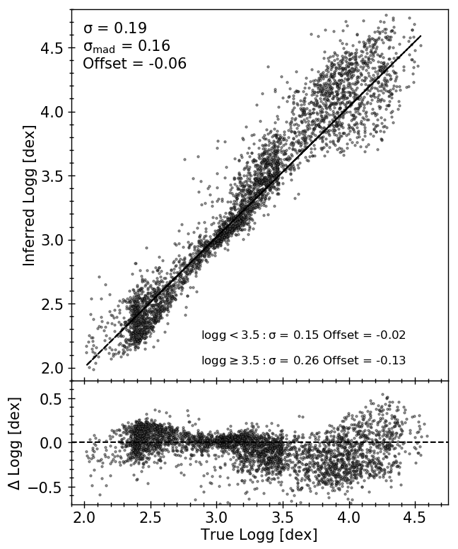
Figure 11: Comparison of inferred surface gravities as a function of reference $\log g$ using The Cannon trained on $\log g$ only. Reference $\log g$ values were obtained from Mathur et al. (2017), Yu et al. (2018) and Berger et al. (2020) for 3,675 stars.

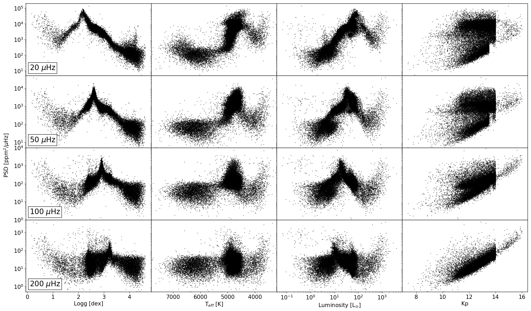
Figure 12: Information content at individual frequencies in the power spectrum plotted for four different labels. Each row corresponds to the power spectral density at a single frequency (ie. 20, 50, 100 and 200 $\mu$Hz), and each column corresponds to a label that we attempted to infer ($\log g$, $T_{\text{eff}}$, luminosity and Kp). This figure demonstrates that for the representative pixels shown, there are relationships between the data and label, but the relationship between the data and the label is not described by a polynomial model over the full range of the data. Over a narrow enough label range, the $\log g$ shows a fairly tight linear relationship with the data amplitude, particularly at lower frequencies.

Figure 10 shows the $\log g$ distribution of the 3,692 stars used in our training set and 3,675 stars used in our testing set. The training set is used to build the model and the test set is used to evaluate its performance in the label inference. The sample was split up in such a way to include sufficient number of stars in the training set to be representative of the parameter range, and contain at least a thousand dwarfs and giants in both the training and testing set.

The training set used to create the model includes a total of 2,437 giants and 1,255 dwarfs (3,692 stars), and was tested on 2,450 giants and 1,225 dwarfs (3,675 stars) (Figure 10). All spectra used for training and testing the model were corrected for white noise following a linear relationship between white noise level and Kepler magnitude.

Figure 11 shows the inference of stellar surface gravity using The Cannon on 3,675 stars with a $\log g$ range of 2.0-4.6 dex. The top panel shows The Cannon’s performance compared to the reference label value and the bottom panel shows the residuals. When trained on $\log g$, The Cannon infers $\log g$ to a precision of 0.16 dex, but with a bias of -0.06 dex. While The Cannon is successfully inferring $\log g$ from the power spectra of light curves, the scatter and bias vary significantly as a function of $\log g$. For instance, it performs worse for subgiants and dwarfs with a scatter of 0.26 dex and a bias of -0.13 dex, and over-predicts $\log g$ for 72% of stars with $\log g$ above 3.5 dex.

Our results using The Cannon with a second order polynomial model demonstrate that while effective across the red giant branch, this approach can not capture well the relationship between time domain variability and the $\log g$ label over a large range of $\log g$ values. A choice of a more flexible model for The Cannon, like a Gaussian process, would possibly circumvent this problem, but at some computational expense, and have lesser interpretability than a (global or local) linear or polynomial modeling approach.

To examine the impact of our choices in The Cannon’s implementation, we trained the model using label combinations such as effective temperature ($T_{\text{eff}}$), luminosity ($L$), Kp and radius. While the model trained on luminosity was slightly successful, the inference failed for the rest of the labels. We also experimented with hyper-parameters such as the number of stars in the reference set, the region and length of the power spectrum used for inference, the region and length of the raw light curve, and specific regions of parameter space. The Cannon is best at predicting $\log g$ when the entire stellar power spectra is used, but we found that it could not match the performance of The Swan.

To understand the better performance of The Swan compared to The Cannon, we examined the correlation between the power spectrum’s amplitude of our reference objects and our labels, including $\log g$, $T_{\text{eff}}$, $L$ and Kp. Figure 12 shows that there are correlations between these labels and the power spectrum amplitude at different frequencies, and that each frequency shows a different label-power amplitude relation. It is clear that these correlations can not be captured with a polynomial model, particularly for the labels of $T_{\text{eff}}$, $L$ and Kp. A local linear model on the other hand, implemented in The Swan, can effectively capture the locally changing relationship between $\log g$ and PSD, over the full range of the data. While the label-PSD correlation is tighter at lower frequencies for $\log g$ in Figure 12 (and note for comparison, is tighter at higher frequencies for Kp), there is information distributed across the full frequency range shown, including up to 200 $\mu$Hz, that can be used to infer $\log g$. We conclude that while The Cannon is a useful method to derive granulation-based $\log g$ for giants, a polynomial model is not sufficiently flexible to model the relationship between the data, and $\log g$ or other labels that describe it, which causes most significant failures in the dwarf and subgiant regime.

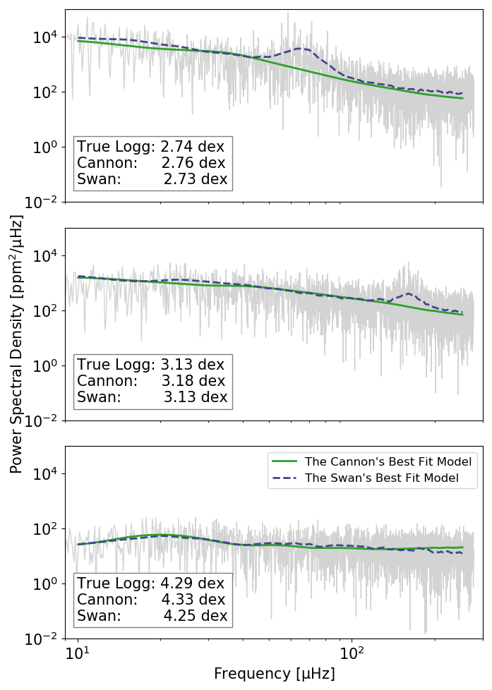
Figure 13: Comparison of The Cannon’s best fit model in green and The Swan’s best fit model in dashed blue for three stars with varying $\log g$. The white noise corrected power spectrum of each star is plotted in grey.

Figure 13 shows additional examples of comparing the The Swan to The Cannon for three stars with different $\log g$ values. For each test star, The Swan’s model captures more of the variance in the data than The Cannon’s global model; it is able to reproduce the variations in the spectral shape in more detail, thus successfully modelling the oscillations when visible. In the bottom panel of Figure 13, we observe that both The Swan and The Cannon’s inferences are close to the reference $\log g$ value for the dwarf star, but The Cannon recovers a systematically higher $\log g$; the polynomial model does not label the data as effectively as The Swan over the full parameter range of the data.

Figure 13 shows that The Swan works better at modeling the power spectra to derive granulation-based $\log g$ measurements. In general, if The Cannon’s model is sufficient to describe the data, it should result in very similar results to a local linear modeling approach. Indeed, the main benefit of The Cannon as used in Ness et al. (2018) compared to a local linear modeling approach may simply be in the lower computational expense, as nearest neighbours do not need to be evaluated and only one model rather than a unique model for each inference, is required.

5 Comparison to Literature

Table 2: Summary of recovered $\log g$ precision for different methods used to infer stellar surface gravity from photometric and spectroscopic data.

$\log g$ Range [dex]	Precision [dex]	Reference	Data Type	Technique
1.0-4.0	0.11-0.22	Ness et al. (2015)	Spectroscopy	The Cannon
1.0-3.5	0.07	Ness et al. (2016)	Spectroscopy	The Cannon
1.0-3.9	0.07	Casey et al. (2016)	Spectroscopy	The Cannon
0.5-4.0	0.10	Ho et al. (2017b)	Spectroscopy	The Cannon
1.0-3.0	0.14	Ting et al. (2017)	Spectroscopy	The Payne
0.8-4.0	0.06	Fabbro et al. (2018)	Spectroscopy	convolution neural networks
0.0-5.0	0.07	Xiang et al. (2019)	Spectroscopy	Data-Driven Payne
0.0-5.0	0.05	Ting et al. (2019)	Spectroscopy	The Payne
1.2-4.8	0.12-0.2	Wheeler et al. (2020)	Spectroscopy	The Cannon
1.0-3.6	0.07	Sit & Ness (2020)	Spectroscopy	The Cannon
0.5-5.0	0.06	Guiglion et al. (2020)	Spectroscopy	convolution neural networks
2.7-4.8	0.10	Rice & Brewer (2020)	Spectroscopy	The Cannon
0.5-5.5	0.09	Zhang et al. (2020)	Spectroscopy	support vector regression
2.5-4.6	0.10-0.20	Bastien et al. (2013, 2016)	Photometry (LC)	Flicker
1.0-4.5	0.04-0.18	Kallinger et al. (2016)	Photometry (ACF)	time-scale
0.1-4.6	0.04-0.10	Bugnet et al. (2018)	Photometry (PS)	random forest
2.0-4.8	0.05	Pande et al. (2018)	Photometry (PS)	time-scale
1.5-3.3	0.10	Ness et al. (2018)	Photometry (ACF)	The Cannon
0.2-4.6	0.02-0.11	THIS WORK	Photometry (PS)	local linear regression

Note. — LC: light curve; PS: power spectrum; ACF: auto-correlation function

5.1 Spectroscopy

Data-driven methods have been employed on large surveys of spectroscopic data to infer stellar labels, including $T_{\text{eff}}$, $\log g$, mass, [Fe/H], and detailed chemical abundances (e.g. Ness et al., 2016; Buder et al., 2018; Leung & Bovy, 2019; Behmard et al., 2019; Birky et al., 2020; Galgano et al., 2020; Sit & Ness, 2020; Rice & Brewer, 2020). Simple data-driven methods, like The Cannon, are particularly useful for ‘label-transfer’ where a high-resolution survey can be used to label a low-resolution survey to high precision compared to prior approaches (e.g. Casey et al., 2016; Ho et al., 2017a; Wheeler et al., 2020). The high-resolution APOGEE survey (R=22,500) delivers $\log g$ to a precision of $\sim$0.02 dex (Ahumada et al., 2020) with $S/N>100$, using comparisons to stellar models with their aspcap pipeline (García Pérez et al., 2016). Using the data-driven approach of The Cannon, a high fidelity aspcap sample has been used to label lower-resolution RAVE (R=8000) stars and LAMOST (R=1000) stars to a precision of $\sim$0.04 dex and $\sim$0.10 dex respectively using stars in common between the surveys (Casey et al., 2016; Ho et al., 2017b).

Further data-driven approaches to infer stellar labels includes convolutional neural networks trained on RAVE DR6 and APOGEE DR13 spectra to recover $\log g$ to a precision of 0.06 dex (Fabbro et al., 2018; Guiglion et al., 2020), and Bayesian artificial neural networks with dropout variation inference trained on APOGEE DR14 data to recover $\log g$ and elemental abundances to $\sim$0.02 dex despite a low SNR (SNR$\sim$50) (Leung & Bovy, 2019). With a non-parametric, neural-net-like functional form, The Payne fits physical spectral models to recover stellar parameters and chemical abundances to high precision (Ting et al., 2017, 2019), and can be combined with The Cannon’s data-driven approach to derive stellar labels (Data-Driven Payne, Xiang et al., 2019). Other methods to recover stellar labels from spectroscopic data include line-by-line differential analysis on high resolution (R=115,000) spectra (Bedell et al., 2018), and support vector regression (SVR) trained on LAMOST and APOGEE spectra (Zhang et al., 2020).

Compared to spectroscopy, the photometric method presented here provides better precision over a larger range of evolutionary states (see Table 2). This is consistent with the fact that $\log g$ information in spectral lines is typically degenerate with other atmospheric parameters such as $T_{\text{eff}}$ and [Fe/H] (Torres et al., 2012), while amplitudes of photometric granulation are predominantly determined by surface gravity (Kjeldsen & Bedding, 2011).

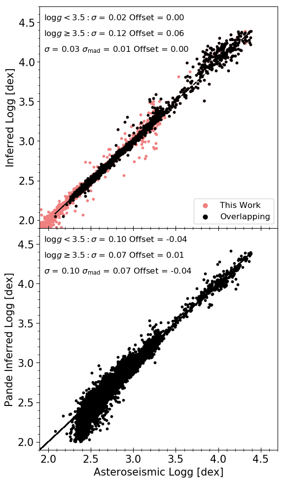
Figure 14: Comparison of The Swan’s performance to the results of Pande et al. (2018) to predict $\log g$ from power spectra for 5,429 stars. Top: Inferred $\log g$ from The Swan versus asteroseismic $\log g$. The red points show the complete seismic sample, and the black points show overlapping stars found in both our seismic sample and Pande et al. (2018). Bottom: Cross-validation of results from Pande et al. (2018) versus asteroseismic $\log g$.

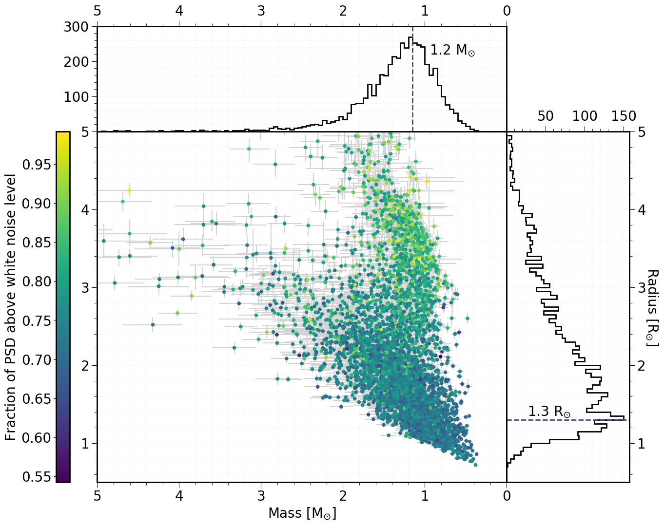
Figure 15: The distribution of masses and radii for Gaia sample using inferred $\log g$ from this work and Gaia derived radii from Berger et al. (2020) to calculate mass. Mass uncertainties are calculated using standard deviation of inferred $\log g$ values and radii errors from Berger et al. (2020). The stars are colour-coded by the fraction of power spectral density above white noise level. There are an additional 111 stars outside of the axis limits.

5.2 Photometry

Using light curves of Kepler stars with stellar surface gravity between 2.5-4.6 dex, Bastien et al. (2013, 2016) inferred $\log g$ from power spectra to $\sim$0.1-0.2 dex precision, by employing the “Flicker” ($F_{8}$) method, which measures stellar variations on time-scales of 8 hours or less, and using asteroseismic samples for calibration (Bruntt et al., 2012; Thygesen et al., 2012; Stello et al., 2013; Huber et al., 2013; Chaplin et al., 2014), but restricted stars with $\log g$ $>$ 2.7 dex. Although they recovered $\log g$ for 27,628 stars, the $F_{8}$ method suffers from a degeneracy where highly evolved stars, or stars with lower $\log g$, may appear as subgiants. Additionally, they find that systematic uncertainties of overlapping red giants-clump stars increase to 0.2 dex; therefore, a red giant with $F_{8}$-inferred $\log g$ between 2.9-3.2 dex may in fact have a true $\log g$ that is $\sim$0.3 dex lower (Bastien et al., 2016).

Kallinger et al. (2016) used typical brightness variations time-scales in Kepler data to infer stellar surface gravities to 4%, by utilizing a self-adapting filter which isolates the gravity-dependent signal from instrumental effects. They employed the auto-correlation function to determine the typical time-scale of the residual signal, and used asteroseismically derived surface gravities across a wide-range of stellar masses and evolutionary states to calibrate their relation. Although they achieved $\log g$ precision of $\sim$0.04-0.18 dex for 1,200 stars, a limitation of their technique is that the time-scale method requires sufficient temporal resolution. Therefore, recovering $\log g$ using their technique on main sequence stars requires short cadence data which are limited given current surveys.

Data-driven approaches have been previously used to determine properties from time-series photometry (e.g. Ness et al., 2018, for red giant stars). Our use of local linear modeling is a marginally more computationally expensive approach compared to The Cannon as used in Ness et al. (2018), but the model flexibility in describing the relationship between time domain data and their labels enables determining stellar properties across evolutionary states.

A recent method to derive $\log g$ from time-series observations was demonstrated in Pande et al. (2018) who derived granulation-based $\log g$ values using the power spectrum rather than the light curve or the auto-correlation function. They measured the granulation background in a limited region of the power spectrum centered at 0.08$\nu_{\text{max}}$ with a fractional width of 20%. For all quarters of Kepler data, they calculated the median granulation power in this region, converted to $\nu_{\text{max}}$ and calculated $\log g$ given a linear relationship between $\log g$ and $\nu_{\text{max}}$ (Kjeldsen & Bedding, 1995).

In the top panel of Figure 14, we compare the results of our approach on the high fidelity asteroseismic stars within the Pande et al. (2018) sample. The bottom panel shows the performance of the Pande et al. (2018) pipeline itself against these reference asteroseismic objects. For 5,429 stars found in both samples, The Swan performs better than the methodology by Pande et al. (2018), with a robust standard deviation of 0.03 dex compared to $\sigma_{\textrm{mad}}$ = 0.10 dex using their method. For subgiants and dwarfs, or stars with $\log g$ $\geq$ 3.5 dex, their analysis yields a marginally better RMS scatter of 0.07 dex compared to our RMS scatter of 0.12 dex. For giants, The Swan performs better with a RMS scatter of 0.02 dex compared to their method which yields a RMS scatter of 0.10 dex.

Interestingly, the bottom panel of Figure 14 shows that Pande et al. (2018) predict a wide range of $\log g$ for a narrow range of giants, seen as a turnoff at $\log g$ $\approx$ 2.4 dex. They used only a part of the power spectrum for their inference, centered at 0.08$\nu_{\text{max}}$ with a fractional width of 20%. Maximum oscillation power for giants is found at lower frequencies; therefore, limiting the spectrum might have made it difficult to differentiate between giants with a range of $\log g$ values. An advantage of our model compared to Pande et al. (2018) is that we use the full spectrum for inference, which allows us to capture granulation over a wide range of evolutionary states. Figure 14 demonstrates that using a restricted region of power spectra prevents successful inference of surface gravity especially for high-luminosity giants. Conversely, we suspect that using the full power spectrum may introduce additional scatter for less evolved stars, for which a smaller fraction of the power spectrum is dominated by granulation.

6 Stellar Masses

Granulation-derived surface gravities in combination with radii from Gaia allow the calculation of stellar masses with little model dependence (Stassun et al., 2018). Therefore, predicting $\log g$ using The Swan enables us to calculate masses for thousands of stars by combining our inferred $\log g$ with Gaia radius (Berger et al., 2020),

$$\text{g}=\text{GM}/\text{R}^{2}$$ (8)

where g is the surface gravity in CGS, R is the stellar radius and G is the gravitational constant.

In Figure 15, we show the distribution of derived masses for the Gaia sample, where the mass ranges from $\sim$0.4-5.3 M_⊙ with a mass peak at 1.2 M_⊙ and a radius peak at 1.3 R_⊙. To calculate mass uncertainties, we used Figure 8 to assign an error to our inferred $\log g$ values while radius uncertainties were obtained from Berger et al. (2020). The mass uncertainty ranges from $\sim$5-47% with a median of $\sim$7%. Only $\sim$1% of stars have a fractional mass uncertainty above 20%. There are 16 stars above 4 M_⊙ which all have a difference between their reference and inferred $\log g$ above 0.33 dex. In fact, $\sim$83% of stars that have a derived mass above 3.5 M_⊙ have a difference between their reference and inferred $\log g$ above 0.25 dex. Such high mass stars are not expected to have convective envelopes, and thus our mass values are very likely overestimated.

In Figure 15, we find a low number of small, high mass stars (bottom left region) since these stars would be rare and found in the post main sequence phase. The curved branch at $\sim$1 M_⊙ for radii above $\sim$2.4 R_⊙ represents subgiant stars. We find a higher density of stars around solar mass and solar radius, which is expected since Kepler was designed to observe solar-type stars (Borucki et al., 2010; Koch et al., 2010). Inferred masses including uncertainties for both the seismic and Gaia samples are provided in Tables 3 and 4, respectively.

7 Conclusions

We presented a simple but effective data-driven approach to predict stellar surface gravity from power spectra of time-series photometry, which we term The Swan. Our main results are as follows:

• We demonstrated that local linear modeling of time-series power spectra can recover stellar surface gravities ($\log g$) to a precision of $\sigma_{\textrm{mad}}$ = 0.02 dex for $\log g$ between 0.2-4.4 dex, when implemented using a reference sample of stars with astroseismically derived $\log g$ (top panel of Figure 1). The Swan infers $\log g$ from the full frequency range of power spectra, and delivers comparable or better precision than previous approaches on time-domain data (e.g. Pande et al., 2018), and spectroscopic data, using e.g. The Cannon (Ness et al., 2015, 2016; Casey et al., 2016; Ho et al., 2017a, b). The Swan maintains high performance across a wide range of evolutionary states.

• We used The Swan to infer stellar surface gravities to a precision of $\sigma_{\textrm{mad}}$ = 0.11 dex, using a reference set of stars with $\log g$ labels derived from isochrone fitting in Berger et al. (2020) to gain larger coverage across evolutionary states (see bottom panel of Figure 1). Using these Gaia derived $\log g$ values leads to a higher scatter and systematic biases for dwarfs compared to reference objects with high precision asteroseismic $\log g$ values. The cause for the higher scatter in this sample could be due to insufficient information for faint, higher $\log g$ stars. Inspection of the recovered fraction as a function of a signal-to-noise metric, or the fraction of power spectral density above white noise level, demonstrated that a lack of detectable granulation leads to an inaccurate $\log g$ measurement. Therefore, granulation-based $\log g$ is likely applicable to very few K dwarfs, and we recommend caution for derived $\log g$ values for any star with low signal-to-noise (faint dwarfs), or stellar radius above 30 R_⊙ (high-luminosity giants).

• We derived empirical masses for 4,646 subgiant and main sequence stars by combining our inferred $\log g$ values with Gaia radii and uncertainties from Berger et al. (2020). We find an average mass of 1.2 M_⊙ representative of the Kepler sample, with a typical uncertainty of 7%. The sample increases the number of model-independent masses over the asteroseismic sample by a factor of 10.

• We tested the effect of photometry baseline on the precision of recovered $\log g$ using The Swan. We demonstrate that the precision remains high ($\sigma<$ 0.15 dex for both samples and $\sigma_{\textrm{mad}}$ $<$ 0.03 dex for the seismic sample) even for 27 day long time-series, which implies that the method can be applied to stars observed by TESS which have sufficiently high enough S/N.

• We also applied The Cannon to power spectra of 3,675 stars and inferred $\log g$ to a precision of $\sigma_{\textrm{mad}}$ = 0.16 dex, a poorer performance compared to The Swan. We find that The Cannon’s use of a polynomial model is not sufficiently flexible to model the relationship between the input data (power spectrum) and $\log g$ over a wide range of evolutionary states.

The Swan code is publicly available at https://github.com/MaryumSayeed/TheSwan and is archived on Zenodo. The methodology presented here can be readily applied to other time-domain surveys such as TESS (Ricker et al., 2014) which observes a much larger number of stars than Kepler. A challenge will be the existence of a sufficiently large reference set, which could be overcome through creation of synthetic light curves, or the detection of oscillations in a sufficient number of dwarfs and subgiants with TESS (Schofield et al., 2019). We also plan to update the model to expand the number of labels we can use for inference from granulation such as stellar metallicity (Corsaro et al., 2017; Tayar et al., 2019), explore which combinations of labels result in a successful inference for other fundamental stellar parameters, and investigate the effect of choosing neighbours on the basis of other stellar parameters. Additional future work includes applying The Swan on light curves from ground-based telescopes like ASASS-N (Kochanek et al., 2017; Auge et al., 2020) and developing similar analyses for stars that exhibit other types of variability (ie. Delta Scutis, RR Lyrae and Gamma Doradus pulsators).

References

- Abdul-Masih et al. (2016) Abdul-Masih, M., Prša, A., Conroy, K., et al. 2016, AJ, 151, 101
- Aerts et al. (2010) Aerts, C., Christensen-Dalsgaard, J., & Kurtz, D. W. 2010, Asteroseismology
- Ahumada et al. (2020) Ahumada, R., Allende Prieto, C., Almeida, A., et al. 2020, ApJS, 249, 3
- Anders et al. (2017) Anders, F., Chiappini, C., Rodrigues, T. S., et al. 2017, A&A, 597, A30
- Anderson et al. (1990) Anderson, E. R., Duvall, Thomas L., J., & Jefferies, S. M. 1990, ApJ, 364, 699
- Astropy Collaboration et al. (2013) Astropy Collaboration, Robitaille, T. P., Tollerud, E. J., et al. 2013, A&A, 558, A33
- Auge et al. (2020) Auge, C., Huber, D., Heinze, A., et al. 2020, AJ, 160, 18
- Baglin et al. (2006) Baglin, A., Auvergne, M., Barge, P., et al. 2006, in ESA Special Publication, Vol. 1306, The CoRoT Mission Pre-Launch Status - Stellar Seismology and Planet Finding, ed. M. Fridlund, A. Baglin, J. Lochard, & L. Conroy, 33
- Bastien et al. (2013) Bastien, F. A., Stassun, K. G., Basri, G., & Pepper, J. 2013, Nature, 500, 427
- Bastien et al. (2016) —. 2016, ApJ, 818, 43
- Bedell et al. (2018) Bedell, M., Bean, J. L., Meléndez, J., et al. 2018, ApJ, 865, 68
- Behmard et al. (2019) Behmard, A., Petigura, E. A., & Howard, A. W. 2019, ApJ, 876, 68
- Belkacem et al. (2011) Belkacem, K., Goupil, M. J., Dupret, M. A., et al. 2011, A&A, 530, A142
- Berger et al. (2018) Berger, T. A., Huber, D., Gaidos, E., & van Saders, J. L. 2018, ApJ, 866, 99
- Berger et al. (2020) Berger, T. A., Huber, D., van Saders, J. L., et al. 2020, arXiv e-prints, arXiv:2001.07737
- Birky et al. (2020) Birky, J., Hogg, D. W., Mann, A. W., & Burgasser, A. 2020, ApJ, 892, 31
- Borucki et al. (2010) Borucki, W. J., Koch, D., Basri, G., et al. 2010, Science, 327, 977
- Boyajian et al. (2013) Boyajian, T. S., von Braun, K., van Belle, G., et al. 2013, ApJ, 771, 40
- Brown & Gilliland (1994) Brown, T. M., & Gilliland, R. L. 1994, ARA&A, 32, 37
- Brown et al. (1991) Brown, T. M., Gilliland, R. L., Noyes, R. W., & Ramsey, L. W. 1991, ApJ, 368, 599
- Brown et al. (2011) Brown, T. M., Latham, D. W., Everett, M. E., & Esquerdo, G. A. 2011, AJ, 142, 112
- Bruntt et al. (2012) Bruntt, H., Basu, S., Smalley, B., et al. 2012, MNRAS, 423, 122
- Buder et al. (2018) Buder, S., Asplund, M., Duong, L., et al. 2018, MNRAS, 478, 4513
- Bugnet et al. (2018) Bugnet, L., García, R. A., Davies, G. R., et al. 2018, A&A, 620, A38
- Casagrande et al. (2014) Casagrande, L., Silva Aguirre, V., Stello, D., et al. 2014, ApJ, 787, 110
- Casey et al. (2016) Casey, A. R., Hogg, D. W., Ness, M., et al. 2016, arXiv e-prints, arXiv:1603.03040
- Casey et al. (2017) Casey, A. R., Hawkins, K., Hogg, D. W., et al. 2017, ApJ, 840, 59
- Chaplin & Miglio (2013) Chaplin, W. J., & Miglio, A. 2013, ARA&A, 51, 353
- Chaplin et al. (2011) Chaplin, W. J., Kjeldsen, H., Bedding, T. R., et al. 2011, ApJ, 732, 54
- Chaplin et al. (2014) Chaplin, W. J., Basu, S., Huber, D., et al. 2014, ApJS, 210, 1
- Choi et al. (2016) Choi, J., Dotter, A., Conroy, C., et al. 2016, ApJ, 823, 102
- Corsaro et al. (2017) Corsaro, E., Mathur, S., García, R. A., et al. 2017, A&A, 605, A3
- De Ridder et al. (2009) De Ridder, J., Barban, C., Baudin, F., et al. 2009, Nature, 459, 398
- Debosscher et al. (2011) Debosscher, J., Blomme, J., Aerts, C., & De Ridder, J. 2011, A&A, 529, A89
- Dotter (2016) Dotter, A. 2016, ApJS, 222, 8
- Evans (2018) Evans, D. F. 2018, Research Notes of the American Astronomical Society, 2, 20
- Fabbro et al. (2018) Fabbro, S., Venn, K. A., O’Briain, T., et al. 2018, MNRAS, 475, 2978
- Fulton & Petigura (2018) Fulton, B. J., & Petigura, E. A. 2018, AJ, 156, 264
- Gaia Collaboration et al. (2018) Gaia Collaboration, Brown, A. G. A., Vallenari, A., et al. 2018, A&A, 616, A1
- Galgano et al. (2020) Galgano, B., Stassun, K., & Rojas-Ayala, B. 2020, AJ, 159, 193
- García et al. (2014) García, R. A., Mathur, S., Pires, S., et al. 2014, A&A, 568, A10
- García Pérez et al. (2016) García Pérez, A. E., Allende Prieto, C., Holtzman, J. A., et al. 2016, AJ, 151, 144
- Guiglion et al. (2020) Guiglion, G., Matijevic, G., Queiroz, A. B. A., et al. 2020, arXiv e-prints, arXiv:2004.12666
- Hastie et al. (2009) Hastie, T., Tibshirani, R., & Friedman, J. H. 2009, The elements of statistical learning: data mining, inference, and prediction, 2nd edn., Springer series in statistics (Springer)
- Hekker & Christensen-Dalsgaard (2017) Hekker, S., & Christensen-Dalsgaard, J. 2017, A&A Rev., 25, 1
- Ho et al. (2017a) Ho, A. Y. Q., Rix, H.-W., Ness, M. K., et al. 2017a, ApJ, 841, 40
- Ho et al. (2017b) Ho, A. Y. Q., Ness, M. K., Hogg, D. W., et al. 2017b, ApJ, 836, 5
- Hogg et al. (2010) Hogg, D. W., Bovy, J., & Lang, D. 2010, arXiv e-prints, arXiv:1008.4686
- Hon et al. (2019) Hon, M., Stello, D., García, R. A., et al. 2019, MNRAS, 485, 5616
- Huber et al. (2011) Huber, D., Bedding, T. R., Stello, D., et al. 2011, ApJ, 743, 143
- Huber et al. (2013) Huber, D., Chaplin, W. J., Christensen-Dalsgaard, J., et al. 2013, ApJ, 767, 127
- Huber et al. (2014) Huber, D., Silva Aguirre, V., Matthews, J. M., et al. 2014, ApJS, 211, 2
- Huber et al. (2017) Huber, D., Zinn, J., Bojsen-Hansen, M., et al. 2017, ApJ, 844, 102
- Hunter (2007) Hunter, J. D. 2007, Computing in Science and Engineering, 9, 90
- Johnson et al. (2010) Johnson, J. A., Aller, K. M., Howard, A. W., & Crepp, J. R. 2010, PASP, 122, 905
- Kallinger et al. (2016) Kallinger, T., Hekker, S., Garcia, R. A., Huber, D., & Matthews, J. M. 2016, Science Advances, 2, 1500654
- Kallinger et al. (2010) Kallinger, T., Mosser, B., Hekker, S., et al. 2010, A&A, 522, A1
- Kjeldsen & Bedding (1995) Kjeldsen, H., & Bedding, T. R. 1995, A&A, 293, 87
- Kjeldsen & Bedding (2011) —. 2011, A&A, 529, L8
- Koch et al. (2010) Koch, D. G., Borucki, W. J., Basri, G., et al. 2010, ApJ, 713, L79
- Kochanek et al. (2017) Kochanek, C. S., Shappee, B. J., Stanek, K. Z., et al. 2017, PASP, 129, 104502
- Leung & Bovy (2019) Leung, H. W., & Bovy, J. 2019, MNRAS, 483, 3255
- Lindegren et al. (2018) Lindegren, L., Hernández, J., Bombrun, A., et al. 2018, A&A, 616, A2
- Mathur et al. (2016) Mathur, S., García, R. A., Huber, D., et al. 2016, ApJ, 827, 50
- Mathur et al. (2011) Mathur, S., Hekker, S., Trampedach, R., et al. 2011, ApJ, 741, 119
- Mathur et al. (2017) Mathur, S., Huber, D., Batalha, N. M., et al. 2017, ApJS, 229, 30
- McKinney (2010) McKinney, W. 2010, in Proceedings of the 9th Python in Science Conference, ed. Stéfan van der Walt & Jarrod Millman, 56 – 61
- McQuillan et al. (2013) McQuillan, A., Aigrain, S., & Mazeh, T. 2013, MNRAS, 432, 1203
- Murphy et al. (2019) Murphy, S. J., Hey, D., Van Reeth, T., & Bedding, T. R. 2019, MNRAS, 485, 2380
- Ness et al. (2015) Ness, M., Hogg, D. W., Rix, H. W., Ho, A. Y. Q., & Zasowski, G. 2015, ApJ, 808, 16
- Ness et al. (2016) Ness, M., Hogg, D. W., Rix, H. W., et al. 2016, ApJ, 823, 114
- Ness et al. (2018) Ness, M. K., Silva Aguirre, V., Lund, M. N., et al. 2018, ApJ, 866, 15
- Pande et al. (2018) Pande, D., Bedding, T. R., Huber, D., & Kjeldsen, H. 2018, MNRAS, 480, 467
- Paxton et al. (2011) Paxton, B., Bildsten, L., Dotter, A., et al. 2011, ApJS, 192, 3
- Paxton et al. (2013) Paxton, B., Cantiello, M., Arras, P., et al. 2013, ApJS, 208, 4
- Paxton et al. (2015) Paxton, B., Marchant, P., Schwab, J., et al. 2015, ApJS, 220, 15
- Pinsonneault et al. (2014) Pinsonneault, M. H., Elsworth, Y., Epstein, C., et al. 2014, ApJS, 215, 19
- Pires et al. (2015) Pires, S., Mathur, S., García, R. A., et al. 2015, A&A, 574, A18
- Rauer et al. (2014) Rauer, H., Catala, C., Aerts, C., et al. 2014, Experimental Astronomy, 38, 249
- Rice & Brewer (2020) Rice, M., & Brewer, J. 2020, arXiv e-prints, arXiv:2007.02942
- Ricker et al. (2014) Ricker, G. R., Winn, J. N., Vanderspek, R., et al. 2014, Society of Photo-Optical Instrumentation Engineers (SPIE) Conference Series, Vol. 9143, Transiting Exoplanet Survey Satellite (TESS), 914320
- Schofield et al. (2019) Schofield, M., Chaplin, W. J., Huber, D., et al. 2019, ApJS, 241, 12
- Silva Aguirre et al. (2015) Silva Aguirre, V., Davies, G. R., Basu, S., et al. 2015, MNRAS, 452, 2127
- Silva Aguirre et al. (2017) Silva Aguirre, V., Lund, M. N., Antia, H. M., et al. 2017, ApJ, 835, 173
- Sit & Ness (2020) Sit, T., & Ness, M. 2020, arXiv e-prints, arXiv:2006.01158
- Stassun et al. (2018) Stassun, K. G., Corsaro, E., Pepper, J. A., & Gaudi, B. S. 2018, AJ, 155, 22
- Stello et al. (2009) Stello, D., Chaplin, W. J., Basu, S., Elsworth, Y., & Bedding, T. R. 2009, MNRAS, 400, L80
- Stello et al. (2013) Stello, D., Huber, D., Bedding, T. R., et al. 2013, ApJ, 765, L41
- Tayar et al. (2019) Tayar, J., Stassun, K. G., & Corsaro, E. 2019, ApJ, 883, 195
- Thompson et al. (2018) Thompson, S. E., Coughlin, J. L., Hoffman, K., et al. 2018, ApJS, 235, 38
- Thygesen et al. (2012) Thygesen, A. O., Frandsen, S., Bruntt, H., et al. 2012, A&A, 543, A160
- Ting et al. (2019) Ting, Y.-S., Conroy, C., Rix, H.-W., & Cargile, P. 2019, ApJ, 879, 69
- Ting et al. (2017) Ting, Y.-S., Rix, H.-W., Conroy, C., Ho, A. Y. Q., & Lin, J. 2017, ApJ, 849, L9
- Torres et al. (2012) Torres, G., Fischer, D. A., Sozzetti, A., et al. 2012, ApJ, 757, 161
- Ulrich (1986) Ulrich, R. K. 1986, ApJ, 306, L37
- van der Walt et al. (2011) van der Walt, S., Colbert, S. C., & Varoquaux, G. 2011, Computing in Science Engineering, 13, 22
- Virtanen et al. (2020) Virtanen, P., Gommers, R., Oliphant, T. E., et al. 2020, Nature Methods, 17, 261
- Wheeler et al. (2020) Wheeler, A., Ness, M., Buder, S., et al. 2020, ApJ, 898, 58
- Xiang et al. (2019) Xiang, M., Ting, Y.-S., Rix, H.-W., et al. 2019, ApJS, 245, 34
- Yu et al. (2018) Yu, J., Huber, D., Bedding, T. R., et al. 2018, ApJS, 236, 42
- Zhang et al. (2020) Zhang, B., Liu, C., & Deng, L.-C. 2020, ApJS, 246, 9