Colour and logarithmic accuracy in final-state parton showers

Abstract

Standard dipole parton showers are known to yield incorrect subleading-colour contributions to the leading (double) logarithmic terms for a variety of observables. In this work, concentrating on final-state showers, we present two simple, computationally efficient prescriptions to correct this problem, exploiting a Lund-diagram type classification of emission regions. We study the resulting effective multiple-emission matrix elements generated by the shower, and discuss their impact on subleading colour contributions to leading and next-to-leading logarithms (NLL) for a range of observables. In particular we show that the new schemes give the correct full colour NLL terms for global observables and multiplicities. Subleading colour issues remain at NLL (single logarithms) for non-global observables, though one of our two schemes reproduces the correct full-colour matrix-element for any number of energy-ordered commensurate-angle pairs of emissions. While we carry out our tests within the PanScales shower framework, the schemes are sufficiently simple that it should be straightforward to implement them also in other shower frameworks.

1 Introduction

Parton showers are ubiquitous tools in high-energy collider physics. In recent years, however, it has become clear that differences between parton showers are among the limiting systematics in many collider physics applications. This has motivated multiple efforts to better understand the consequences of the approximations contained within parton showers, and to exploit that understanding to guide their further development.

The majority of today’s most commonly used showers, in particular those of the dipole family Gustafson:1987rq , make use of the idea of approximating QCD as if it had a large number of colours ($N_{\text{{c}}}$). Within this approximation one can view each event as a collection of independent colour dipoles: each gluon in an event functions as the colour-triplet end of one dipole and the colour anti-triplet end of another, while each (anti-)quark is the colour (anti-)triplet end of a single dipole. Those dipoles then radiate independently (and incoherently) from each other. This makes it relatively straightforward, at each stage of the showering, to generate a radiation pattern that is correct across small and large angles in the large-$N_{\text{{c}}}$ limit.

There are several ongoing efforts to include subleading-$N_{\text{{c}}}$ corrections, for example Refs. Platzer:2012np ; Nagy:2012bt ; Nagy:2015hwa ; Platzer:2018pmd ; Nagy:2019pjp ; Forshaw:2019ver ; DeAngelis:2020rvq ; Hoeche:2020nsx ; Holguin:2020oui . Including subleading colour corrections in full generality turns out to be computationally challenging, because as the parton multiplicity increases one should keep track of a rapidly-growing number of possible colour configurations, with contributions from higher-dimensional colour representations. Here we explore a complementary approach, one which connects the questions of subleading colour and subleading logarithmic contributions.

To help make things concrete, let us recall the PanScales criteria Dasgupta:2018nvj ; Dasgupta:2020fwr for assessing the logarithmic accuracy of a shower

1. We should identify the kinematic configurations for which a shower correctly reproduces tree-level squared matrix elements. Typically it is useful to discuss this as a function of the separation between emissions in a Lund diagram Andersson:1988gp . We return to this in more detail in section 2.

2. We should evaluate the logarithmic accuracy of the shower’s predictions for a range of common observables. Suppose we calculate some property $P(\alpha_{s},L)$ of an event, where $\alpha_{s}$ is the strong coupling at a scale close to the hard scale, $Q$, of the event, and $L$, which we take negative throughout this paper, is the logarithm of a ratio of scales. For example this might be the cross section for events whose thrust is larger than $1-e^{-|L|}$, or it might be the number of subjets found when clustering the event with resolution scale $Q^{2}e^{-2|L|}$. There are two ways of classifying logarithmic accuracy.

   1. For observables that exponentiate (typically event shapes and some jet rates), one can organise logarithmically enhanced terms as follows Catani:1992ua :

      $$\mbox{}P(\alpha_{s},L)=P(\alpha_{s},0)\exp\!\Bigg{(}\!\underbrace{\alpha_{s}^{-1}g_{1}(\alpha_{s}L)}_{\text{LL}}\,+\,\underbrace{g_{2}(\alpha_{s}L)}_{\text{NLL}}\,+\,\underbrace{\alpha_{s}g_{3}(\alpha_{s}L)}_{\text{NNLL}}+\cdots\!\!\Bigg{)}+{\cal O}\left(e^{-|L|}\right).$$ (1)

      LL stands for leading-logarithmic accuracy, NLL for next-to-leading logarithmic, and so forth. The N^kLL functions, $\alpha_{s}^{k-1}g_{k+1}(\alpha_{s}L)$, resum terms $\alpha_{s}^{n}L^{n+1-k}$ and may in some cases involve operators rather than numbers. The LL function, $\alpha_{s}^{-1}g_{1}(\alpha_{s}L)$, starts off with a double logarithmic term $\alpha_{s}L^{2}$. Certain observables, such as fragmentation functions and energy flow into a limited angular region, start only from the $g_{2}$ function, (in much of the literature, the $g_{2}$ function is then called LL; for consistency across the full set of observables, here we still call it NLL).

   2. For other observables, for example subjet multiplicities and certain other jet rates, there is no simple exponentiation of double logarithmic (DL) terms, and one may instead write

      $$\mbox{}P(\alpha_{s},L)=P(\alpha_{s},0)\Bigg{(}\!\!\underbrace{h_{1}(\alpha_{s}L^{2})}_{\text{DL}}\,+\,\underbrace{\alpha_{s}^{1/2}h_{2}(\alpha_{s}L^{2})}_{\text{NDL}}\,+\,\underbrace{\alpha_{s}h_{3}(\alpha_{s}L^{2})}_{\text{NNDL}}+\cdots\!\!\Bigg{)}+{\cal O}\left(e^{-|L|}\right)\!,$$ (2)

      where the N^kDL function, i.e. $\alpha_{s}^{k/2}h_{k+1}(\alpha_{s}L^{2})$, resums terms $\alpha_{s}^{n}L^{2n-k}$. In other work, this classification is often called N^kLL (or occasionally N^kLL_Σ). We adopt the N^kDL nomenclature here to avoid confusion with the N^kLL of Eq. (1).

For both the matrix element and observable-resummation logarithmic accuracy criteria, one may keep track of powers of the number of colours. Making the number of colours explicit, the leading-colour (LC) part of the LL function, LL-LC, involves terms $\alpha_{s}^{n}N_{\text{{c}}}^{n}L^{n+1}$, while the next-to-leading colour (NLC) part, LL-NLC, involves terms $\alpha_{s}^{n}N_{\text{{c}}}^{n-2}L^{n+1}$ and so forth. When needed, we will use the abbreviation FC to explicitly denote contributions that include the full colour structure.

Standard dipole showers correctly capture the full set of LL-LC terms (or DL-LC terms, as appropriate for the event property being measured). For exponentiating event properties, it is natural to consider values of the logarithm down to $L\sim-1/\alpha_{s}$ where NLL terms are of order 1 (cf. Eq. (1)). Keeping in mind that, numerically, $\alpha_{s}\sim 1/N_{\text{{c}}}^{2}\sim 0.1$, one then concludes that LL-NLC and NLL-LC terms are of comparable importance. For observables that do not exponentiate, one instead considers values of the logarithm down to $L\sim-1/\sqrt{\alpha_{s}}$, and with the same $\alpha_{s}\sim 1/N_{\text{{c}}}^{2}$ equivalence, one may take DL-NLC terms to be comparable to NNDL-LC terms.

Recently there has been significant progress in designing classes of showers that are NLL and NDL (LC) accurate aside from spin correlations, and in numerically demonstrating that accuracy in practice Dasgupta:2020fwr (Refs. Nagy:2020rmk ; Nagy:2020dvz instead examine an analytical approach). An approach that bears similarities to one of those shower classes was discussed in Ref. Forshaw:2020wrq . At this point, to consistently control all first subleading aspects beyond the LL-LC approximation, it becomes essential to identify approaches to construct showers that are correct not just at NLL-LC, but also LL-NLC (such approaches tend also to bring DL-NLC accuracy).

In this paper, we present two related, simple approaches whose colour handling goes beyond LL-LC/DL-LC accuracy. Both approaches are based on the observation that colour coherence (or equivalently, angular ordering) provides an understanding of the colour structure for emissions in phase-space regions that involve disparate angles. Specifically, when angles are disparate, one can use colour coherence to identify the colour factor for radiation, either $C_{F}$ if all emissions at smaller angles form a net colour (anti-)triplet, or $C_{A}$ if they form a net colour octet.

The relevant information can be organised with the help of Lund diagrams. The potential to use Lund diagrams and colour coherence to understand the structure of colour assignment in dipole branching was pointed out long ago by Gustafson Gustafson:1992uh , with a concrete scheme proposed in Ref. Friberg:1996xc (section 4.2). However, subsequent dipole showers adopted different schemes, which have since been found to generate spurious LL-NLC terms in some cases Dasgupta:2018nvj (cf. also Refs. BryanUnpublished ; NagySoperUnpublished ).

The two schemes that we develop, which are computationally efficient, will achieve NDL-FC and NLL-FC accuracy for multiplicities and global event shapes respectively, thus going beyond the accuracy of the scheme proposed in Ref. Friberg:1996xc . For non-global logarithms (which start at NLL in our counting), they are NLL-FC accurate only up to some fixed order (${\cal O}\left(\alpha_{s}\right)$ or ${\cal O}\left(\alpha_{s}^{2}\right)$, depending on the scheme), however they are in good numerical agreement with the full-colour all-order computation of Hatta and Ueda Hatta:2013iba , to within the latter’s few-percent accuracy. For many practical purposes, therefore, it seems that our colour schemes have sufficient accuracy not just for NDL/NLL showers, but even as a basis for use in potential future NNDL/NNLL showers (where the colour terms left out by our schemes will be commensurate with N³LL leading-colour terms).

This article is structured as follows. In section 2 we will recall how Lund diagrams can be used to understand the assignment of $C_{F}$ and $C_{A}$ colour factors and then, in sections 3 and 4, introduce two concrete schemes that can be straightforwardly applied to a range of 21st century dipole showers. For reference, in section 5 we will briefly review the standard colour scheme in modern dipole showers. Then in section 6 we shall carry out a set of numerical tests, comparing the effective tree-level matrix elements being generated by our schemes to known exact results in energy-ordered limits. In section 7 we will examine a range of observables, using both standard colour assignment schemes and our new schemes, comparing the results to known DL-FC and NDL-FC, as well as LL-FC and NLL-FC expectations.

2 Angular ordering and Lund diagrams

Let us start by elaborating on the first of our two criteria for logarithmic accuracy, i.e. the reproduction of matrix elements in suitably ordered limits. It is convenient to use Lund diagrams as a way of visualising the phase-space (see Ref. Dreyer:2018nbf for a concrete prescription to construct the Lund diagram from an event’s kinematics). At LL accuracy, the tree-level matrix elements should be correct for any number of emissions that are well separated in a Lund diagram in both the logarithm of transverse momentum ($k_{t}$) and in rapidity ($\eta=-\ln\tan\theta/2$), which one might call double strong ordering; at NLL accuracy, the tree-level matrix elements should be correct for any number of emissions that are well separated in at least one direction in the Lund diagram. Well-separated means that the distance $D$ between points in the Lund diagram corresponding to any given pair of emissions should satisfy $e^{-D}\ll 1$. The correctness of the matrix element should hold no matter what that direction is, e.g. some may be well separated in rapidity but have similar $\ln k_{t}$, while others may be well separated in $\ln k_{t}$ but have similar $\eta$ values. In this article, the only respect in which we will relax this requirement on (leading-colour) logarithmic accuracy concerns the treatment of azimuthal correlations in collinear splittings, as induced by spin correlations, a topic that we defer to future work.

Throughout this section and the next ones, we will discuss how we attribute the correct colour factor for real emissions. The reader should keep in mind that virtual contributions are also being implicitly corrected at the same time, a consequence of the unitary nature of the showers that we consider in this paper.

For subleading colour effects at LL accuracy, one only needs to obtain the correct tree-level matrix element in regions where emissions are all well separated in rapidity. In this limit, for radiation at an angle $\theta$, the question of colour reduces to that of examining the set of partons contained within a cone of aperture $\theta$ around the dipole end that is closer in angle. If that cone contains a single net quark (or anti-quark), i.e. $|n_{q}-n_{\bar{q}}|=1$, then the radiation is associated with a $C_{F}=(N_{\text{{c}}}^{2}-1)/(2N_{\text{{c}}})$ colour factor, while if the cone contains zero net quarks, the radiation is associated with a $C_{A}=N_{\text{{c}}}$ colour factor. In the limit where all emissions are well separated in rapidity, these are the only two possible situations, and there will also never be any partons close to the edge of a given cone (because then the radiation would end up close in rapidity to an existing parton, keeping in mind that $g\to q{\bar{q}}$ splittings are implicitly collinear up to and including NLL accuracy).

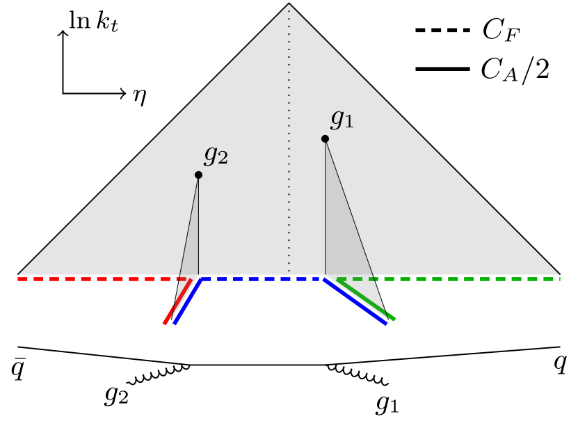
(a)

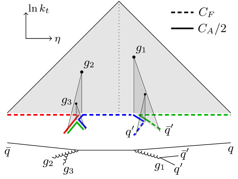
(b)

Figure 1: Two example events and associated Lund diagrams. Points in the Lund diagram represent branchings, the triangles represent the two-dimensional logarithmic phase-space, while the coloured lines at the base of the diagram represent the phase-space for individual colour-dipoles (at the corresponding $k_{t}$ value), with dashed and solid segments indicating the parts of the dipole that should be associated respectively with a $C_{F}$ versus a $C_{A}/2$ colour factor.

Although it is informative to refer to angular cones, it is more practical, going forwards, to use Lund diagrams. The angular-ordered colour-assignment prescription is illustrated with Lund diagrams in Fig. 1 for two $e^{+}e^{-}\to\bar{q}q$ events, each dressed with additional radiation. Recall that the main large triangle corresponds to the phase-space associated with the original $e^{+}e^{-}\to\bar{q}q$ event (primary Lund plane), while each “leaf” that comes away from the main plane represents the additional phase-space that becomes available following emissions from that $q\bar{q}$ system (for example radiation collinear to the gluon in a ${\bar{q}}qg$ system). For concreteness we imagine a transverse momentum-ordered shower and consider the state of the event at a value of the ordering variable $k_{t}$ corresponding to the lower edge of the diagram (though our arguments apply to a range of shower ordering choices). The phase-space for emission at that $k_{t}$ is given by the base of the Lund diagram.

Let us first consider Fig. 1(a). In a normal leading-$N_{\text{{c}}}$ picture, this event consists of three colour dipoles: ${\bar{q}}g_{2}$, $g_{2}g_{1}$ and $g_{1}q$, represented as red, blue and green solid/dashed lines at the base of the Lund diagram. The dashed and solid styles indicate the colour factor based on angular ordering, which we work through in the rest of this paragraph. Along the dashed part of the (red) ${\bar{q}}g_{2}$ dipole, i.e. the part on the primary Lund plane, any subsequent gluon emission is closer in angle to the ${\bar{q}}$ than to $g_{2}$ and a cone drawn around the ${\bar{q}}$ contains just the ${\bar{q}}$, so the colour factor is $C_{F}$. Along the solid part of the dipole, i.e. the part on the leaf associated with $g_{2}$, the cone should be drawn around the gluon $g_{2}$, since that is the dipole end that is closer in angle. The only particle contained within the cone around $g_{2}$ is the gluon $g_{2}$ itself, and one should use a colour factor of $C_{A}/2$.

Next, we consider the (blue) $g_{2}g_{1}$ dipole. In the solid blue region, along $g_{2}$’s leaf, the cone is to be drawn around $g_{2}$ and the only particle that is contained is a gluon, so we have a $C_{A}/2$ colour factor; the situation is analogous for the solid blue region along $g_{1}$’s leaf. For the part of the dipole that is dashed, along the primary Lund plane, we need to separately examine the parts to the left and the right of the vertical dotted line. To the left, $g_{2}$ is the end of the dipole that is closer in angle. Writing the angle of the radiation, $r$, with respect to $g_{2}$ as $\theta_{rg_{2}}$, and keeping in mind that we are in a region of the Lund plane were $\theta_{rg_{2}}\gg\theta_{{\bar{q}}g_{2}}$, the cone of angle $\theta_{rg_{2}}$ that we draw around $g_{2}$ automatically contains ${\bar{q}}$ as well as $g_{2}$, so the colour factor is $C_{F}$. The situation is similar to the right of the vertical dotted line, but with a cone containing $g_{1}$ and $q$. Finally the (green) $g_{1}q$ dipole can be understood in analogy with the (red) ${\bar{q}}g_{2}$ dipole.

Based on the above reasoning it is relatively straightforward to see that if one has an arbitrarily large number of gluon emissions (including secondary gluon emissions, but no $g\to q\bar{q}$ splittings), then to determine the colour factor, one should identify whether an emission is on the primary Lund plane and if it is assign a $C_{F}$ colour factor, otherwise assign a $C_{A}/2$ colour factor. That was the key observation made long ago by Gustafson Gustafson:1992uh . A specific scheme (based on boosts) for achieving this was incorporated Friberg:1996xc as a modification of the Ariadne parton shower Andersson:1988gp ; Lonnblad:1992tz .

The next question one may ask is what happens if one allows for $g\to{\bar{q}}q$ splittings. Whether one should consider this to be part of the LL terms is a matter that one may debate: on one hand $g\to{\bar{q}}q$ splittings can exist in double-strongly ordered configurations. On the other hand if one integrates over their phase-space (as is relevant for thinking about logarithmically enhanced contributions to common observables), each $g\to{\bar{q}}q$ splitting contributes only a single logarithm, i.e. an effect that is at most NLL in our counting. Here, we take the view that we should favour the (slightly) more ambitious goal and so aim to obtain the correct colour factors for double-strongly ordered configurations including $g\to{\bar{q}}q$ splittings. Such a configuration is shown in Fig. 1(b) and observing the (blue) $g_{3}q^{\prime}$ dipole, one sees that it consists of a sequence of solid ($C_{A}/2$) and dashed ($C_{F}$) segments, with the final dashed segment along the $q^{\prime}$ leaf, which is not part of the primary Lund plane. In general the number of segments on a dipole can be anywhere between $1$ (e.g. the solid green $g_{2}g_{3}$ dipole) and infinity, though in practice the average number of segments per dipole turns out to be of order $1$ even in high-multiplicity events, a consequence of the smaller number of quarks than gluons produced in the parton shower. This picture differs from the standard approach within dipole showers of breaking every dipole into two parts, each associated with one of the two ends. Note that in this paper we will apply our new segmentation just for the purposes of colour assignment, retaining the default two-part segmentation for the kinematic maps of each shower that we examine.

3 A solution with segments and transition points

Based on the reasoning in section 2, here we propose the first of our concrete schemes for achieving LL full-colour accuracy. We start by introducing the key ideas with the help of a worked example, section 3.1. We then discuss choices we can make that affect aspects beyond LL-FC accuracy, section 3.2, or that arise in occasional special cases, section 3.3 (some readers may prefer to skip these parts). In section 3.4 we give our full algorithm. Finally in section 3.5 we show how it can be adapted to the Pythia 8 shower Sjostrand:2004ef ; Sjostrand:2014zea .

3.1 A worked example

The key insight from section 2 is that to obtain LL full colour accuracy it is enough to break every dipole into a suitable sequence of $C_{F}$ and $C_{A}$ colour segments. We label those segments by their extremities in rapidity and the colour factor along the segment. For an initial $e^{+}e^{-}\to{\bar{q}}q$ event we start with a single dipole consisting of one segment stretching from a rapidity of $\eta=-\infty$ (${\bar{q}}$ end) to $\eta=+\infty$ ($q$ end), associated with a $C_{F}$ colour factor. We denote this as

$$[-\infty,C_{F},\infty]_{\bar{q}q}\,,$$ (3)

where our notation consists of a sequence of segment boundaries (or, equivalently, transition points) and segment colour factors. When a dipole emits a gluon $g_{1}$, we define the gluon’s rapidity within the dipole, $\eta_{g_{1}}=\pm|\ln\tan\theta/2|$, in terms of its angle $\theta$ with respect to the dipole end that is closer in the event frame. We assign a positive (negative) rapidity if it is closer to the triplet (anti-triplet) end. Since there is only a $C_{F}$ segment in the $\bar{q}q$ dipole, the gluon is necessarily emitted with a $C_{F}$ colour factor.

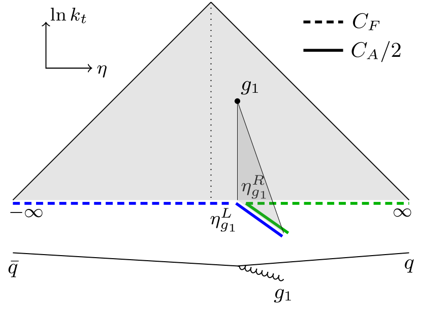
(a)

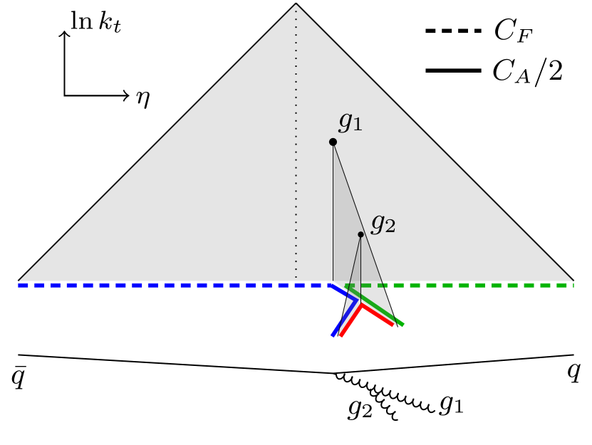
(b)

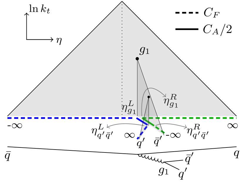
(c)

Figure 2: Examples of colour segments and transition points for representative configurations: (a) a $q\to qg$ splitting (i.e. the emission of a gluon from a quark segment), (b) a $g\to gg$ splitting (i.e. a gluon emission from a gluon segment), and (c) a $g\to q\bar{q}$ splitting.

When we radiate a gluon $g_{1}$ from the ${\bar{q}}q$ dipole, we end up with two dipoles, ${\bar{q}}g_{1}$ and $g_{1}q$, each of which now has one $C_{F}$ and one $C_{A}$ region, cf. Fig. 2(a). The segmentation for the two dipoles is as follows

$$[-\infty,C_{F},\color[rgb]{0,0,1}\eta_{g_{1}}^{L},C_{A},\infty]_{\bar{q}g_{1}}+[-\infty,C_{A},\eta_{g_{1}}^{R},\color[rgb]{0,0,0}C_{F},\infty]_{g_{1}q}\,,$$ (4)

where we have highlighted in blue the extra segments that are a consequence of the gluon emission and, for now, we take $\eta_{g_{1}}^{L}\equiv\eta_{g_{1}}^{R}\equiv\eta_{g_{1}}$. We see here that both new dipoles have a transition point at the rapidity of the emission itself (see Fig. 2(a)). Note that since gluons are shared across two dipoles, the second segment should really have a colour factor $C_{A}/2$. For compactness, we suppress the explicit factor $1/2$ in our notation.

Next, we consider a second emission, $g_{2}$. It is sufficient to examine the situation where it is emitted from the ${\bar{q}}g_{1}$ dipole. We use the same procedure to evaluate the rapidity $\eta_{g_{2}}$ of $g_{2}$ as given above, but now with respect to the ${\bar{q}}g_{1}$ dipole, and we examine where $\eta_{g_{2}}$ lies in the ${\bar{q}}g_{1}$ sequence of segments. Since there are two segments, there are two possible cases: (a) $-\infty<\eta_{g_{2}}<\eta_{g_{1}}^{L}$, where radiation occurs with a $C_{F}$ colour factor and (b) $\eta_{g_{1}}^{L}<\eta_{g_{2}}<\infty$ where it occurs with a $C_{A}/2$ colour factor. As well as differing in the colour factor for emission, the two cases also differ in terms of the resulting set of new segments. Case (a), emission from the $C_{F}$ region, gives the following segmentation of the resulting three dipoles

$$[-\infty,C_{F},\color[rgb]{0,0,1}\eta_{g_{2}}^{L},C_{A},\infty]_{\bar{q}g_{2}}+[-\infty,C_{A},\eta_{g_{2}}^{R},\color[rgb]{0,0,0}C_{F},\eta_{g_{1}}^{L},C_{A},\infty]_{g_{2}g_{1}}+[-\infty,C_{A},\eta_{g_{1}}^{R},C_{F},\infty]_{g_{1}q},$$ (5)

i.e. one splits the ${\bar{q}}g_{1}$ sequence of segments in Eq. (4) into two separate sequences: one is for the ${\bar{q}}g_{2}$ dipole, which keeps everything to the left of the $C_{F}$ segment where the radiation occurred, plus a closing $\color[rgb]{0,0,1}\eta_{g_{2}}^{L},C_{A},\infty]$ right segment; and one for the $g_{2}g_{1}$ dipole, which keeps everything to the right of the $C_{F}$ segment, plus a closing $\color[rgb]{0,0,1}[-\infty,C_{A},\eta_{g_{2}}^{R}$ left segment. This pattern corresponds exactly to what we see in Fig. 1(a). Case (b), insertion into the $C_{A}$ region, is shown in Fig. 2(b) and gives

$$[-\infty,C_{F},\eta_{g_{1}}^{L},C_{A},\color[rgb]{0,0,1}\infty]_{\bar{q}g_{2}}+[-\infty,\color[rgb]{0,0,0}C_{A},\infty]_{g_{2}g_{1}}+[-\infty,C_{A},\eta_{g_{1}}^{R},C_{F},\infty]_{g_{1}q}\,.$$ (6)

Again we have highlighted the new part in blue. Since we are inserting a gluon into a $C_{A}$ region there are no additional $C_{F}{-}C_{A}$ transition points.

The final case that we need to consider is the splitting of a gluon to $q^{\prime}{\bar{q}}^{\prime}$, cf. Fig. 2(c). In a strong ordering (i.e. collinear) limit, as relevant for accuracies up to and including NLL, the $|\eta|$ associated with the $g\to q^{\prime}\bar{q}^{\prime}$ splitting will always be larger than the last non-infinite $\eta$ transition point in each dipole’s sequence, i.e. the splitting will always be associated with a $C_{A}$ segment that is at the extreme left or right ends of a sequence. We consider a ${\bar{q}}g_{1}q$ event and the branching of $g_{1}\to q^{\prime}\bar{q}^{\prime}$ in the ${\bar{q}}g_{1}$ dipole, i.e. we have Eq. (4) as our starting point. Defining

$$\eta^{L}_{q^{\prime}\bar{q}^{\prime}}=-\eta^{R}_{q^{\prime}\bar{q}^{\prime}}=|\eta_{q^{\prime}\bar{q}^{\prime}}|\,,\qquad\eta_{q^{\prime}\bar{q}^{\prime}}\equiv-\ln\tan\theta_{q^{\prime}\bar{q}^{\prime}}/2\,,$$ (7)

where $\theta_{q^{\prime}\bar{q}^{\prime}}$ is the opening angle of the $q^{\prime}\bar{q}^{\prime}$ pair in the event frame, we then obtain the following segments

$$[-\infty,C_{F},\eta_{g_{1}}^{L},C_{A},\color[rgb]{0,0,1}\eta^{L}_{q^{\prime}\bar{q}^{\prime}},C_{F},\infty]_{\bar{q}q^{\prime}}+[-\infty,C_{F},\eta^{R}_{q^{\prime}\bar{q}^{\prime}},\color[rgb]{0,0,0}C_{A},\eta_{g_{1}}^{R},C_{F},\infty]_{\bar{q}^{\prime}q}.$$ (8)

i.e. the ${\bar{q}}g_{1}$ and $g_{1}q$ dipoles have respectively become ${\bar{q}}q^{\prime}$ and ${\bar{q}}^{\prime}q$ dipoles and each of those dipoles has additional transition points to a $C_{F}$ colour factor at $\eta^{L}_{q^{\prime}\bar{q}^{\prime}}=|\eta_{q^{\prime}\bar{q}^{\prime}}|$ and $\eta^{R}_{q^{\prime}\bar{q}^{\prime}}=-|\eta_{q^{\prime}\bar{q}^{\prime}}|$ respectively. The opposite signs for $\eta^{L}_{q^{\prime}\bar{q}^{\prime}}$ and $\eta^{R}_{q^{\prime}\bar{q}^{\prime}}$ arise because the transition needs to be at angles close to the $q^{\prime}$ for the ${\bar{q}}q^{\prime}$ dipole, i.e. positive rapidity, and at angles close to the ${\bar{q}}^{\prime}$ end of the ${\bar{q}}^{\prime}q$ dipole, i.e. negative rapidity.

Before formulating a full, concrete algorithm, some details need to be specified, related to ${\cal O}\left(1\right)$ choices for the rapidity boundaries (section 3.2), and the handling of cases where two emissions are close in rapidity, with resulting ambiguities in how to construct the segments (section 3.3).

3.2 Specific rapidity definitions and NDL accuracy

There are two aspects to examine concerning the exact choices of rapidity transition points, both relevant for configurations where two branchings occur at similar angles. One involves identifying a choice that can provide full-colour NDL (NDL-FC) accuracy for basic quantities like jet and particle multiplicities, i.e. control of terms $\alpha_{s}^{n}L^{2n-1}$. The control of this class of terms at NDL-FC accuracy has long been one of the strong arguments in favour of angular ordered showers Marchesini:1983bm . The other question is more practical: in the segment algorithm we implicitly assume that all transition points are ordered, with a consistent alternating set of $C_{F}$ and $C_{A}$ segments. Those properties are trivially maintained when all branchings are at disparate angles, but that is no longer necessarily the case when two or more branchings are at commensurate angles.

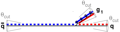
Figure 3: Illustration of the configuration that we consider to examine the equivalence between exact angular ordering and our partitioning of dipoles, as relevant for NDL accuracy in particle and jet multiplicities. We will consider the emission of a further soft gluon, $g_{2}$, with respect to this configuration, at an angle of at least $\theta_{\text{cut}}$ away from the ${\bar{q}}$, $q$ and $g_{1}$. The dashed/solid coloured lines indicate schematically where we use a $C_{F}$ v. $C_{A}/2$ colour factor for each of the two dipoles (blue: ${\bar{q}}g_{1}$, red $g_{1}q$).

We first consider what is required for NDL-FC accuracy. We start with a system ${\bar{q}}g_{1}q$, with $\theta_{g_{1}q}\ll 1$, and examine the emission of a second much softer gluon, $g_{2}$, in a limited range of energy, $\Delta\!\ln E$, and with the following angular constraints:

$$\{\theta_{g_{2}q},\theta_{g_{2}{\bar{q}}},\theta_{g_{2}g_{1}}\}>\theta_{\text{cut}}\,.$$ (9)

The angular limits for the emission of $g_{2}$ are represented schematically in Fig. 3 and we work in a limit where $\theta_{\text{cut}}\ll\theta_{g_{1}q}$. The integrated full-colour rate of $g_{2}$ emission in this region is well known to be Dokshitzer:1991wu ; Ellis:1991qj

$$I_{\text{FC}} =\frac{2\alpha_{s}\,\Delta\!\ln E}{\pi}\left[2C_{F}\ln\frac{2}{\theta_{\text{cut}}}+C_{A}\ln\frac{\theta_{g_{1}q}}{\theta_{\text{cut}}}\right],$$ (10a)

$$=\frac{2\alpha_{s}\,\Delta\!\ln E}{\pi}\left[2C_{F}\eta_{\text{cut}}+C_{A}(\eta_{\text{cut}}-\eta_{g_{1}})\right],$$ (10b)

where $\eta_{g_{1}}=-\ln\tan\theta_{g_{1}q}/2$, $\eta_{\text{cut}}=-\ln\tan\theta_{\text{cut}}/2$. The parton shower’s ability to reproduce this result is a key requirement for NDL full-colour accuracy. In particular, if the evaluation of this integrated emission rate for the shower has an extra ${\cal O}\left(1\right)$ constant in the square bracket, NDL accuracy will not be achieved.

To provide a concrete demonstration of how to satisfy Eq. (10), we consider the PanScales showers Dasgupta:2020fwr . The kinematics for branching in these showers is parameterised in terms of the shower ordering variable $\ln v$, a longitudinal variable $\bar{\eta}$ (linearly related to the logarithm of a light-cone momentum component) and an azimuthal angle $\phi$. The emission density (working at fixed coupling for illustrative purposes) is

$$C\frac{2\alpha_{s}}{\pi}d\bar{\eta}\,d\ln v\frac{d\phi}{2\pi}\,,$$ (11)

where $C$ is the colour factor ($C_{F}$ or $C_{A}$ with $C_{F}=C_{A}/2$ in the large-$N_{\text{{c}}}$ limit). To integrate the shower over the region of Eq. (9), one needs to relate $\bar{\eta}$ to the actual rapidity of a soft and collinear emission from a dipole $ij$ with respect to the closer of $i$ and $j$. The following approximate formula (specific to the PanScales showers)

$$\eta_{\text{approx}}^{(ij)}=\left\{\begin{array}[]{lll}\bar{\eta}-\frac{1}{2}\ln\left(\frac{1-\cos\theta_{ij}}{2}\right)\,,&&\bar{\eta}>0\,,\\ \bar{\eta}+\frac{1}{2}\ln\left(\frac{1-\cos\theta_{ij}}{2}\right)\,,&&\bar{\eta}<0\,,\end{array}\right.$$ (14)

provides the (signed) rapidity with respect to the closer of $i$ and $j$ (when the dipole for which we evaluate $\eta_{\text{approx}}$ is obvious, we omit the $(ij)$ superscript). It is approximate in the following sense: for an emission $k$ from an $ij$ dipole, the true rapidity with respect to the closer of $i$ and $j$ has additional ${\cal O}\left(1\right)$ corrections when the smaller of the $\theta_{ik}$ and $\theta_{jk}$ is commensurate with $\theta_{ij}$. For a soft emission, those corrections vanish when the ratio of $\min(\theta_{ik},\theta_{jk})$ to $\theta_{ij}$ is small. This is the case notably close to the $\theta_{\text{cut}}$ limits in Eq. (9).

For the configuration in Fig. 3, with $\theta_{g_{1}q}\ll 1$ ($\theta_{{\bar{q}}g_{1}}\simeq\pi$), we have

$$\bar{q}g_{1} \eta_{\text{approx}}^{({\bar{q}}g_{1})}=\bar{\eta}\,,$$ dipole: (15a)

$$g_{1}q \eta_{\text{approx}}^{(g_{1}q)}=\left\{\begin{array}[]{lll}\bar{\eta}+\eta_{g_{1}}&&\bar{\eta}>0\,,\\ \bar{\eta}-\eta_{g_{1}}&&\bar{\eta}<0\,.\end{array}\right.$$ dipole: (15d)

Note that $\eta_{\text{approx}}$ depends linearly on $\bar{\eta}$ except at $\bar{\eta}=0$, where it is discontinuous for the $g_{1}q$ (i.e. small-angle) dipole. With these results one can translate the constraints of Eq. (9) into constraints on $\bar{\eta}$ for each of the two dipoles,

$$\bar{q}g_{1} -\eta_{\text{cut}}<\bar{\eta}<\eta_{\text{cut}}\,,$$ dipole: (16a)

$$g_{1}q -\eta_{\text{cut}}+\eta_{g_{1}}<\bar{\eta}<\eta_{\text{cut}}-\eta_{g_{1}}\,.$$ dipole: (16b)

For each of the dipoles, the procedure of section 3.1 splits the dipole’s rapidity range into a $C_{F}$ piece and a $C_{A}/2$ piece. The choice that we make for the transition points is $\bar{\eta}=\eta_{g_{1}}$ for the ${\bar{q}}g_{1}$ dipole (using $C_{F}$ for $\bar{\eta}<\eta_{g_{1}}$), and $\bar{\eta}=0$ for the $g_{1}q$ dipole (using $C_{F}$ for $\bar{\eta}>0$). Together with the limits in Eq. (16), one then finds that the $C_{A}/2$ pieces from the two dipoles add up to give a total $\bar{\eta}$ range of $2(\eta_{\text{cut}}-\eta_{g_{1}})$, while the $C_{F}$ pieces add up to give $2\eta_{\text{cut}}$, giving a total result for the parton shower of

$$I_{\text{PS}}=\frac{2\alpha_{s}\,\Delta\!\ln E}{\pi}\left[2C_{F}\eta_{\text{cut}}+C_{A}(\eta_{\text{cut}}-\eta_{g_{1}})\right],$$ (17)

in agreement with the full-colour result of Eq. (10).

While the discussion in terms of $\bar{\eta}$ is useful for locating an emission with respect to a dipole with a single transition point, to handle more complicated events, it becomes simpler to reason directly in terms of $\eta_{\text{approx}}$. Thus the transition point for the ${\bar{q}}g_{1}$ dipole is at $\eta_{\text{approx}}=\eta_{g_{1}}$. For the $g_{1}q$ dipole, since $\eta_{\text{approx}}$ is discontinuous at $\bar{\eta}=0$, any transition between $-\eta_{g_{1}}$ and $+\eta_{g_{1}}$ is equivalent. One simple convention is to set the transition for the $g_{1}q$ dipole to be at $\eta_{\text{approx}}=0$, i.e. along the dipole’s angular bisector in the event frame.

Together, these observations bring us to the following recipe for soft emission from a configuration with an existing collinear branching. Working in the event centre-of-mass frame, when inserting a gluon emission $i$ into a $C_{F}$ segment, determine its angle $\theta_{i}$ to the triplet (anti-triplet) end of the dipole if $\eta_{\text{approx},i}>0$ ($<0$) and define $\eta_{i}=\mp\ln\tan\theta_{i}/2$, using a negative (positive) sign when the $\theta_{i}$ is determined with respect to the triplet (anti-triplet) end. In constructing new transition points, e.g. as in Eqs. (4) or (5), use

$$\eta^{L}_{i}=\max\left(0,\eta_{i}\right)\,,\quad\eta^{R}_{i}=\min\left(0,\eta_{i}\right)\,.$$ (18)

When considering the generation of a new emission $k$, determine its $\eta_{\text{approx},k}$ from Eq. (14) and compare that $\eta_{\text{approx},k}$ to the dipole’s existing transition points to determine the segment to which the emission belongs and the associated $C_{F}$ v. $C_{A}/2$ colour factor.

Similar considerations about the total integral for soft gluon emission are relevant for a $g\to{\bar{q}}q$ splitting. One can demonstrate that the prescription given in Eqs. (7) and (8) already ensures the correct integral, an analogue of Eq. (10).

3.3 Special cases

When inserting a gluon $g$ into a $C_{F}$ segment, and that gluon’s angle with respect to the dipole end is close to an existing transition point, it can sometimes happen that the insertion $\eta_{g}^{L}$ or $\eta_{g}^{R}$ lies outside the segment range (recall that $\eta_{\text{approx}}$ and $\eta_{\text{exact}}$ can differ by an order $1$ amount when the emission angle is commensurate with the dipole opening angle). From a DL logarithmic point of view, e.g. for particle or jet multiplicities, such a situation is beyond NDL. Specifically, to trigger it, one must have two energy-ordered gluons at similar angles. In such a situation, any subleading-$N_{\text{{c}}}$ issue induced by mis-ordering of transition points only affects emission of a subsequent, third, soft gluon that is once again at a similar angle (it also affects related virtual corrections). The requirement of three energy-ordered gluons at commensurate angles corresponds to NNDL terms for quantities such as multiplicities, because one loses a logarithm relative to DL for each of the second and third gluons when requiring its angle to be similar to the first.

Still, we need a definite prescription to handle such cases. We choose to give priority to the requirement that the transition points in the colour-segment sequence should always remain ordered. Consider the configuration $[\ldots,C_{A},\eta_{i-1},C_{F},\eta_{i},C_{A}\ldots]_{ab}$ and a situation where we have located a new emission, according to its $\eta_{\text{approx}}$, as belonging to the central $C_{F}$ segment. We would normally expect to split the sequence as

$$[\ldots,C_{A},\eta_{i-1},C_{F},\eta_{i},C_{A}\ldots]_{ab}\to[\ldots,C_{A},\eta_{i-1},C_{F},\color[rgb]{0,0,1}\eta_{g}^{L},C_{A},\infty]_{ag}+\\ \color[rgb]{0,0,1}+[-\infty,C_{A},\eta_{g}^{R},\color[rgb]{0,0,0}C_{F},\eta_{i},C_{A},\ldots]_{gb}\,,$$ (19a)

but if $$\eta_{g}^{L}\leq\eta_{i-1} ag \eta_{i-1},C_{F},\eta_{g}^{L} \eta_{g}^{L},C_{A},\infty C_{A} +\infty$$, we discard the last two segments of the new sequence ( and ) and extend the remaining rightmost segment to ,

$$[\ldots,C_{A},\eta_{i-1},C_{F},\eta_{i},C_{A}\ldots]_{ab}\to[\ldots,C_{A},\color[rgb]{0,0,1}\infty]_{ag}+[-\infty,C_{A},\eta_{g}^{R},\color[rgb]{0,0,0}C_{F},\eta_{i},C_{A},\ldots]_{gb}\,.$$ (19b)

We use an analogous procedure when $\eta_{g}^{R}\geq\eta_{i}$, dropping the two first segments of the $gb$ sequence and extending its leftmost $C_{A}$ segment to $-\infty$. Since $\eta_{g}^{L}\geq\eta_{g}^{R}$, and since the transition points are always ordered prior to insertion, this adaptation is needed at most on one side, never both.

Similar considerations apply to $g\to q\bar{q}$ splittings, though the impact on accuracy is now only expected to be N³DL, because $g\to q\bar{q}$ splittings start one logarithm down. Where normally we would have

$$[\ldots,C_{F},\eta_{i},C_{A},\infty]_{ag}+[-\infty,C_{A},\eta_{j},C_{F},\ldots]_{gb}\to\\ [\ldots,C_{F},\eta_{i},C_{A}\color[rgb]{0,0,1},\eta^{L}_{q^{\prime}\bar{q}^{\prime}},C_{F},\infty]_{aq^{\prime}}+[-\infty,C_{F},\eta^{R}_{q^{\prime}\bar{q}^{\prime}},\color[rgb]{0,0,0}C_{A},\eta_{j},C_{F},\ldots]_{{\bar{q}}^{\prime}b}\,,$$ (20a)

if $$\eta_{q^{\prime}{\bar{q}}^{\prime}}^{L}\leq\eta_{i} aq^{\prime} C_{F}$$, then we remove the last two segments of the new sequence and extend its remaining rightmost () segment to infinity,

$$[\ldots,C_{F},\eta_{i},C_{A},\infty]_{ag}+[-\infty,C_{A},\eta_{j},C_{F},\ldots]_{gb}\to\\ [\ldots,C_{F},\color[rgb]{0,0,1}\infty]_{aq^{\prime}}+[-\infty,C_{F},\eta^{R}_{q^{\prime}\bar{q}^{\prime}},\color[rgb]{0,0,0}C_{A},\eta_{j},C_{F},\ldots]_{{\bar{q}}^{\prime}b}\,.$$ (20b)

There is an analogous adaptation when $\eta^{R}_{q^{\prime}\bar{q}^{\prime}}\geq\eta_{j}$.

In practice, for physical $\alpha_{s}$ values, these adaptations are used in at most a few percent of gluon insertions in $C_{F}$ segments and for up to $10{-}20\%$ of $g\to q{\bar{q}}$ splittings.

3.4 The algorithm

With the help of the above reasoning we are now ready to formulate a full segment-based algorithm for the PanScales showers. The event should start with Eq. (3) for an initial $e^{+}e^{-}\to{\bar{q}}q$ event and analogues with $C_{A}$ for the two dipoles of an initial $H\to gg$ event. Splitting functions and their integrals for Sudakov factors should by default all be evaluated with the replacement $C_{F}\to C_{A}/2=N_{\text{{c}}}/2$. Dipoles are always labelled by their anti-triplet end followed by their triplet end.

For emission of a gluon $g$ from an $ab$ dipole, use the parent dipole momenta and PanScales kinematic generation variable $\bar{\eta}$ to determine $\eta_{\text{approx}}^{(ab)}$ for the gluon, according to Eq. (14). Identify the location of $\eta_{\text{approx}}^{(ab)}$ within the $ab$ dipole’s sequence of segments. If it is in a $C_{F}$ segment, reject the emission with probability $(1-2C_{F}/C_{A})$ (or, alternatively, multiply the event weight by $(1-2C_{F}/C_{A})$). If it is rejected, continue by generating the next value for the shower ordering variable, starting from the value that was been rejected. If the emission is accepted, and $\eta_{\text{approx}}^{(ab)}>0$ ($<0$) evaluate $\eta_{g}=-\ln\tan\theta_{gb}/2$ ($\ln\tan\theta_{ag}/2$). Determine $\eta_{g}^{L}$ and $\eta_{g}^{R}$ from $\eta_{g}$ according to Eq. (18), and replace the $ab$ dipole’s sequence of segments with new sequences for the $ag$ and $gb$ dipoles as follows,

$$[\ldots,C_{F},\ldots]_{ab}\to[\ldots,C_{F}\color[rgb]{0,0,1},\eta_{g}^{L},C_{A},\infty]_{ag}+[-\infty,C_{A},\eta_{g}^{R},\color[rgb]{0,0,0}C_{F},\ldots]_{gb}\,.$$ (21)

The left and right “$\ldots$” represent the full sequences to the left and right ends of the original $C_{F}$ factor. They are assigned respectively to the left and right ends of the $ag$ and $gb$ dipoles’ sequences. If $\eta_{g}^{L}$ is such that its insertion would create a disordered sequence of transition rapidities, remove the last two segments in the $ag$ dipole, i.e. use Eq. (19b). Proceed analogously for $\eta_{g}^{R}$.

If the emitted gluon’s $\eta_{\text{approx},g}$ is in a $C_{A}$ segment, do not apply any additional rejection factor (i.e. generate the gluon with its original $C_{A}/2$ colour factor) and replace the $ab$ dipole sequence of segments as follows.

$$[\ldots,C_{A},\ldots]_{ab}\to[\ldots,C_{A}\color[rgb]{0,0,1},\infty]_{ag}+[-\infty,\color[rgb]{0,0,0}C_{A},\ldots]_{gb}\,,$$ (22)

where the $C_{A}$ on the left corresponds to the segment associated with $\eta_{\text{approx},g}$.

Finally we consider $g\to q^{\prime}{\bar{q}}^{\prime}$ splitting, where the gluon belongs to two dipoles $ag$ and $gb$. We assume the splitting to have been generated with a normal $P_{g\to q{\bar{q}}}$ splitting function, so there is no rejection factor to apply. Using the opening angle $\theta_{q^{\prime}{\bar{q}}^{\prime}}$ between the new quark and anti-quark, determine $\eta^{L}_{q^{\prime}\bar{q}^{\prime}}=-\eta^{R}_{q^{\prime}\bar{q}^{\prime}}=|\ln\tan\theta_{q^{\prime}{\bar{q}}^{\prime}}/2|$, i.e. Eq. (7). The $g\to q^{\prime}{\bar{q}}^{\prime}$ splitting then acts as follows on the segments:

$$[\ldots,C_{A},\infty]_{ag}+[-\infty,C_{A},\ldots]_{gb}\to[\ldots,C_{A}\color[rgb]{0,0,1},\eta^{L}_{q^{\prime}\bar{q}^{\prime}},C_{F},\infty]_{aq^{\prime}}+[-\infty,C_{F},\eta^{R}_{q^{\prime}\bar{q}^{\prime}},\color[rgb]{0,0,0}C_{A},\ldots]_{{\bar{q}}^{\prime}b}\,.$$ (23)

In a situation where the insertion of $\eta^{L}_{q^{\prime}\bar{q}^{\prime}}$ would lead to a disordered sequence of transition points, remove the last two segments from the $aq^{\prime}$ dipole, as in Eq. (20b), and analogously remove the first two segments from the ${\bar{q}}^{\prime}b$ dipole if $\eta^{R}_{q^{\prime}\bar{q}^{\prime}}$ is disordered with respect to the other transition points.

3.5 Use in other showers, e.g. Pythia 8

The technique outlined above can be applied to almost any dipole or antenna shower. The one adaptation that is required is to identify a suitable expression for $\eta_{\text{approx}}$, i.e. the analogue of Eq. (14), for that shower. For example in the Pythia 8 shower Sjostrand:2004ef ; Sjostrand:2014zea , for a dipole $ab$ where the emitter has momentum ${\widetilde{p}}_{b}$ and the spectator ${\widetilde{p}}_{a}$, the expression for $\eta_{\text{approx}}$ is

$$\eta_{\text{approx}}^{(ab)}=\left\{\begin{array}[]{lll}\eta_{\text{approx}}^{b}&=\ln 2{\widetilde{p}}_{b}.Q-\frac{1}{2}\ln(Q^{2}p_{\perp\text{evol}}^{2})+\ln(1-z)\,,&\eta_{\text{approx}}^{b}\geq-\eta_{\text{approx}}^{a}\,,\\[5.0pt] \eta_{\text{approx}}^{a}&=-\ln\frac{2{\widetilde{p}}_{a}.Q}{2{\widetilde{p}}_{a}.{\widetilde{p}}_{b}}-\frac{1}{2}\ln\frac{p_{\perp\text{evol}^{2}}}{Q^{2}}+\ln(1-z)\,,&\eta_{\text{approx}}^{b}<-\eta_{\text{approx}}^{a}\,,\end{array}\right.$$ (24)

where $p_{\perp\text{evol}}$ is the shower evolution variable (a transverse momentum), the event momentum is $Q$, and $1-z$ is the fraction of ${\widetilde{p}}_{b}$’s energy carried away by the gluon in the dipole centre-of-mass frame. One can verify that when an emission is soft and collinear to one of ${\widetilde{p}}_{b}$ or ${\widetilde{p}}_{a}$, this gives the correct signed rapidity with respect to the closer of $b$ or $a$ in the event centre-of-mass frame.

4 A solution with nested ordered double-soft (NODS) corrections

The approach of section 3 had two elements: one was the determination of an effective colour factor for each new emission; the other was to establish whether a new emission should be attributed to a $C_{F}$ segment from the point of view of the colour-factor identification for subsequent emissions.

In this section we consider an approach that retains the second of these elements, but replaces the binary colour-factor choice ($C_{F}$ v. $C_{A}/2$) with a local matrix-element correction that reproduces the full-$N_{\text{{c}}}$ radiation pattern for configurations involving a pair of energy-ordered soft gluons that are close in rapidity in the Lund diagram, but with all other emissions well separated in rapidity from them and from each other. The procedure will actually give the correct full-$N_{\text{{c}}}$ matrix element even when there are multiple such pairs around, as long as each is well separated in rapidity from all others (in the same sense as in our discussion at the beginning of section 2).

As in the previous section, we will start by explaining our general approach in the case of a simple subset of event structures in section 4.1. Next, in section 4.2, we will consider issues that arise for more general event structures. We will then give our complete algorithm in section 4.3.

4.1 Angular-ordered primary-only events

To understand the NODS procedure, consider a situation with a single ${\bar{q}}q$ pair and gluons $g_{1}\ldots g_{n}$, each of which is primary in the Lund-diagram sense and well separated in rapidity from all the other gluons, with an ordering in Lund-diagram primary rapidity of $\eta_{1}\ll\eta_{2}\ll\ldots\ll\eta_{n}$. This configuration will dominantly be associated with a leading-colour dipole structure ${\bar{q}}1$, $12$, $23$, $\ldots$, $nq$ (up to corrections suppressed by powers of $e^{-|\eta_{i}-\eta_{j}|}$), which we can represent as

using $n=4$ for concreteness. The corresponding leading-colour squared matrix element for emission of a soft gluon with momentum $k$ is

$$|M_{\text{LC}}|^{2}=\frac{C_{A}}{2}\left[({\bar{q}}1)+(12)+(23)+\ldots+(nq)\right]\,,$$ (26)

where we have introduced the shorthand

$$(ab)\equiv 16\pi\alpha_{s}\frac{2p_{a}.p_{b}}{(2p_{a}.k)(2k.p_{b})}\propto\frac{1-\cos\theta_{ab}}{(1-\cos\theta_{ak})(1-\cos\theta_{kb})}\,,$$ (27)

and assigned a $C_{A}/2$ colour factor to each dipole. In the specific limit that we are considering, i.e. primary emissions that are all well separated in rapidity, the full-colour matrix element reduces to

$$|M|^{2}=|M_{\text{LC}}|^{2}+\left(C_{F}-\frac{C_{A}}{2}\right)({\bar{q}}q)\,.$$ (28)

One simple approach to reproducing Eq. (28) would be to introduce an acceptance probability for each emission of

$$p^{\text{accept}}=\frac{|M|^{2}}{|M_{\text{LC}}|^{2}}\,.$$ (29)

We will introduce a general shorthand for such expressions

$$p^{\text{accept}}({\bar{q}},1,2,\ldots,n,q)\equiv 1+\left(\frac{2C_{F}-C_{A}}{C_{A}}\right)\frac{({\bar{q}}q)}{({\bar{q}}1)+(12)+\ldots+(nq)}\,.$$ (30)

One approach along these lines was proposed in Ref. Giele:2011cb . A downside of any approach that uses the full set of momenta in the acceptance is that for an $N$-particle event it would involve evaluating ${\cal O}\left(N\right)$ dot products for each emission, leading to a contribution to the total showering time that scales as $N^{2}$. This is not necessarily prohibitive; for example the implementation of the Pythia 8 showering algorithm scales as $N^{2}$, and showers with global recoil such as PanGlobal also scale as $N^{2}$ in their current implementation. However it turns out to be possible to formulate an expression for $p_{\text{accept}}$ that maintains the same accuracy but can be evaluated in ${\cal O}\left(1\right)$ time.

To understand how this can be done, we consider a dipole in the middle of the chain, say $i,i+1$, where both $i$ and $i+1$ are gluons. Specifically for this dipole we are free to use

$$|M_{\text{LC},i,i+1}|^{2} =\frac{C_{A}}{2}\left[(i-1,i)+(i,i+1)+(i+1,i+2)\right]\,,$$ (31a)

$$|M_{i,i+1}|^{2} =|M_{\text{LC},i,i+1}|^{2}+\left(C_{F}-\frac{C_{A}}{2}\right)(i-1,i+2)\,,$$ (31b)

$$p^{\text{accept}}_{i,i+1} =\frac{|M_{i,i+1}|^{2}}{|M_{\text{LC},i,i+1}|^{2}}\equiv p^{\text{accept}}(i-1,i,i+1,i+2)\,,$$ (31c)

rather than the full $p^{\text{accept}}({\bar{q}},1,2,\ldots,n,q)$. In $|M_{\text{LC}}|^{2}$ we are justified in dropping all dipoles ${\bar{q}}1$, …, $(i-2,i-1)$, and $(i+2,i+3)$, …, $nq$, because of the requirement that all emissions are well separated in rapidity. To see this, imagine that $i$ is at negative rapidity ($\theta_{{\bar{q}}i}\ll 1$), $i+1$ is at positive rapidity ($\theta_{i+1,q}\ll 1$). Consider an emitted gluon $k$ such that $\theta_{ik}\simeq\theta_{{\bar{q}}i}$. Then, because of our requirement that all existing emissions should be well separated in rapidity, we have $\theta_{i-2,i-1}\ll\theta_{i-2,k}\simeq\theta_{i-1,k}$. Examining Eq. (27) one can then see that the $(i-2,i-1)$ term is negligible compared to the terms included in $|M_{\text{LC},i,i+1}|^{2}$, which is simply a consequence of the fact that a small-angle dipole does not substantially emit at large angles. Similarly for the $(i+2,i+3)$ term, as well as all the other terms that we have neglected in Eq. (31a). Now we turn to Eq. (31b): here we have replaced a ${\bar{q}}q$ with $i-1,i+2$, which is justified since $\theta_{i-1,k}-\theta_{{\bar{q}},k}\ll\theta_{{\bar{q}}k}$ and $\theta_{k,i+2}-\theta_{k,q}\ll\theta_{kq}$ for any momentum $k$ that is likely to be radiated by the $(i,i+1)$ dipole.

Note that with the truncation adopted in Eq. (31a), it would not be sensible to use the $({\bar{q}}q)$ emission factor in the $(C_{F}-C_{A}/2)$ term of Eq. (31b), because such a term would have a negative divergence for $k$ exactly collinear to ${\bar{q}}$ or $q$ that would not be compensated for by any of the terms in the $|M_{\text{LC},i,i+1}|^{2}$ contribution. In contrast, one can show that the acceptance probability as written Eq. (31) is bounded to be in the range

$$1-3\left(\frac{C_{A}-2C_{F}}{C_{A}}\right)=1-\frac{3}{N_{\text{{c}}}^{2}}\leq p^{\text{accept}}_{i,i+1}\leq 1\,,$$ (32)

i.e. for the physical value of $N_{\text{{c}}}$ it is always positive definite and so straightforward to use in event generation.

We have given the justification for writing Eq. (31) in a specific frame, one in which it is manifest that one can replace ${\bar{q}}$ with $i-1$ and $q$ with $i+2$. However the underlying expressions are Lorentz invariant, and the validity of those replacements is ultimately ensured by the condition that all existing emissions are on the primary Lund plane and separated by large differences in rapidity.

We also need to consider dipoles at the end of the chain, for example the ${\bar{q}}1$ dipole in Eq. (25). In such a case, we simply write

$$p^{\text{accept}}_{{\bar{q}},1}=p^{\text{accept}}({\bar{q}},1,2)\,,$$ (33)

and analogously at the other extremity.

In what follows, when we write

$$p^{\text{accept}}_{i,i+1}=p^{\text{accept}}(i-1;i,i+1;i+2)\,,$$ (34)

it is useful to introduce the following terminology: $i-1$ is the auxiliary momentum at the colour-anti-triplet ($i$) end of the dipole, and $i+2$ is the auxiliary at the colour-triplet ($i+1$) end of the dipole. We have emphasised that $i-1$ and $i+2$ are auxiliaries by separating their indices from the others with semi-colons. One can then represent the event of Eq. (25) as

where the dotted line beneath each solid black dipole represents the $-1/(2N_{\text{{c}}})$ dipole that we use in the matrix-element correction. It shows, for example, that the $23$ dipole has auxiliaries $1$ and $4$, leading to an acceptance factor $p^{\text{accept}}(1;2,3;4)$.

4.2 Considerations for general events

Most events do not consist just of angular-ordered primary emissions discussed so far: primary gluons can themselves emit secondary gluons, and any gluon may split to $q\bar{q}$.

The first case that we consider is emission from a region that would be associated with a $C_{F}$ colour factor in the segment approach, e.g. the emission of $5$ from the $23$ dipole,

$$\scalebox{0.7}{\includegraphics[valign={c}]{diagrams/primary-dipoles-auxiliaries.pdf}}\quad\longrightarrow\scalebox{0.7}{\includegraphics[valign={c}]{diagrams/primary-dipoles-CFemsn-auxiliaries.pdf}}$$ (36)

When $5$ is well-separated in rapidity from both $2$ and $3$, the acceptance factor for emission of $5$ will reduce to $2C_{F}/C_{A}$. The new $25$ dipole retains the left-hand auxiliary ($1$) of the parent dipole and acquires a new right-hand auxiliary ($3$), corresponding to the triplet end of the parent dipole. Similarly, the new $53$ dipole acquires a new left-hand auxiliary ($2$), corresponding to the anti-triplet end of the parent dipole, and retains the parent’s right-hand auxiliary ($4$).

Next, we consider a collinear $g\to gg$ splitting. Imagine that we have the configuration in Eq. (35) and that dipole $23$ branches, with its $2$ end splitting to gluons $5$ and $6$ in a collinear configuration $\theta_{56}\ll\theta_{15}\simeq\theta_{16}$, illustrated as follows

$$\scalebox{0.7}{\includegraphics[valign={c}]{diagrams/primary-dipoles-auxiliaries.pdf}}\quad\longrightarrow\scalebox{0.7}{\includegraphics[valign={c}]{diagrams/primary-dipoles+split-auxiliaries.pdf}}$$ (37)

where the new $56$ dipole is highlighted in red. The $15$ dipole, which is the successor of the $12$ dipole retains the $12$ dipole’s auxiliaries. Similarly the $63$ dipole retains the $23$ dipole’s auxiliaries. The new $56$ dipole, since it is produced far in Lund-plane rapidity from any region with a $2C_{F}/C_{A}$ correction, does not need any auxiliaries, in the same way that it has no transitions points (and so no $C_{F}$ segments) in the approach of section 3.

For configurations that are not strongly ordered, e.g. emission of $5$ from the $23$ dipole at an angle that is commensurate with $\theta_{21}$, the acceptance factor is unambiguous (and correct) in our approach. However there is an ambiguity in the assignment of auxiliaries to the child dipoles, which translates to an ambiguity in the acceptance for a subsequent third emission at similar angles, a configuration where we do not aim for full-$N_{\text{{c}}}$ accuracy. We resolve that ambiguity as follows: as well as retaining information on auxiliaries, we also retain information on segments and their transitions, as in the approach of section 3. If an emission occurs in a $C_{F}$ segment then we assign new auxiliaries as in Eq. (36). Instead, if it occurs in a $C_{A}/2$ segment, we do not introduce any new auxiliaries, as in Eq. (37).

Finally, we consider a $g\to q^{\prime}{\bar{q}}^{\prime}$ splitting (for which we always assign a normal $P_{g\to q{\bar{q}}}$ splitting function and use a colour acceptance factor of $1$). Consider $2\to q^{\prime}{\bar{q}}^{\prime}$,

$$\scalebox{0.7}{\includegraphics[valign={c}]{diagrams/primary-dipoles-auxiliaries.pdf}}\quad\longrightarrow\scalebox{0.7}{\includegraphics[valign={c}]{diagrams/primary-dipoles+qqbar-auxiliaries.pdf}}$$ (38)

where we have highlighted the new $q^{\prime}{\bar{q}}^{\prime}$ pair in red. To justify the choice for the new auxiliary variables, we consider the radiation of a soft gluon after the $2\to q^{\prime}\bar{q}^{\prime}$ splitting. In the segmented approach of section 3 we would have said that that the ${\bar{q}}^{\prime}3$ dipole now has two $C_{F}$ segments. In our NODS approach, we introduce an acceptance factor for each $C_{F}$-like segment in the dipole and determine the overall acceptance for the dipole as the product of the individual acceptance factors. E.g. for the ${\bar{q}}^{\prime}3$ dipole we write

$$p^{\text{accept}}_{{\bar{q}}^{\prime},3}=p^{\text{accept}}({\bar{q}}^{\prime},3;q^{\prime})\,p^{\text{accept}}(1;{\bar{q}}^{\prime},3;4)\,,$$ (39)

where the first $C_{F}$-like segment starting from the ${\bar{q}}^{\prime}$ is associated with a single auxiliary ($q^{\prime}$), at its right-hand end, while the second $C_{F}$ segment retains the auxiliaries of the parent $23$ dipole. For strongly angular-ordered configurations, i.e. $\theta_{q^{\prime}{\bar{q}}^{\prime}}\ll\theta_{q^{\prime}1}$, only one of the two $p^{\text{accept}}(\ldots)$ factors in Eq. (39) will ever differ substantially from $1$. For configurations where strong angular ordering does not hold, for which we do not aim to achieve full-$N_{\text{{c}}}$ accuracy, there will be phase-space regions for a subsequent emission $k$ where both factors will be below $1$.

4.3 Full algorithm

We are now ready to specify our full matrix-element-based NODS colour-handling algorithm. It retains the core framework of the segmented approach, specified in section 3.4, with the following augmentations:

1. Where the extremity of a segment has finite rapidity, it is associated with an auxiliary, which we denote $\bar{a}$ towards the anti-triplet end of the segment and $a$ towards the triplet end.

2. Emission acceptance:

   1. The acceptance for gluon emission from a dipole $ij$ is the product of individual acceptance factors for each of the dipole’s $C_{F}$ segments. The individual acceptance factor for a given $C_{F}$ segment is

      $$p^{\text{accept}}_{\text{segment}}=p^{\text{accept}}([\bar{a}];i,j;[a])\,,$$ (40)

      where $p^{\text{accept}}([\bar{a}];i,j;[a])$ is evaluated using Eq. (30). The auxiliary momenta are in square brackets to indicate that if the segment does not have the corresponding auxiliary, because its extremity stretches to infinite rapidity, $p^{\text{accept}}$ is to be evaluated without that auxiliary. For example, in the case with no auxiliaries at either end, the acceptance reduces to $p^{\text{accept}}(i,j)\equiv 2C_{F}/C_{A}$.

   2. For a $g\to q^{\prime}\bar{q}^{\prime}$ splitting, the colour acceptance factor is set to 1.

3. Auxiliaries update:

   1. If a gluon emission $k$ from an $ij$ dipole occurs in a $C_{F}$ segment with auxiliaries $\bar{a}$ and $a$, then the corresponding $C_{F}$ segment in the child $ik$ dipole has auxiliaries $\bar{a}$ and $j$, while that in the child $kj$ dipole has auxiliaries $i$ and $a$. (Where an auxiliary is absent in the parent dipole because the segment stretches to infinite rapidity, it remains absent in the child dipole).

   2. If a gluon emission from an $ij$ dipole occurs in a $C_{A}$ segment, the child dipoles’ $C_{F}$ segments retain the auxiliaries of the parent dipole.

   3. For $g\to q^{\prime}\bar{q}^{\prime}$ splitting, the new $C_{F}$ segment in the anti-triplet-$q^{\prime}$ dipole acquires the ${\bar{q}}^{\prime}$ as its anti-triplet (left) end auxiliary, while the new segment in the ${\bar{q}}^{\prime}$-triplet dipole acquires $q^{\prime}$ as its triplet (right-hand) end auxiliary.

   4. In those special cases of the algorithm of section 3.4 where two segments are removed from the extremity of a sequence, the corresponding auxiliaries are also to be removed.

When storing the auxiliary for a segment, there is some freedom: for example one can choose the auxiliary’s momentum at the time that it is associated with the segment, or its (possibly different) momentum at a later stage in the event when one is evaluating Eq. (40). In practice we make a third choice: when gluon emission causes a left-hand auxiliary to be first added to a segment-sequence of an $ij$ dipole, we store the difference in direction between the auxiliary and the anti-triplet end of the dipole, $\delta_{i\bar{a}}=d_{\bar{a}}-d_{i}$, where $d_{i}$ is the 3-vector direction of $i$. For a right-hand auxiliary point, we store the difference in direction between the auxiliary and the triplet end of the dipole $\delta_{ja}=d_{a}-d_{j}$. When we later come to need an auxiliary momentum to evaluate Eq. (40) in an $\ell m$ dipole that descends from the original $ij$, we reconstruct auxiliary directions using differences with respect to the $\ell$ and $m$ directions at that stage of the event,

$$p^{\text{accept}}_{\text{segment}}=p^{\text{accept}}(\delta_{i\bar{a}}+d_{\ell};\ell,m;\delta_{ja}+d_{m})\,.$$ (41)

For a $g\to q^{\prime}{\bar{q}}^{\prime}$ splitting, in the $C_{F}$ segment on the anti-triplet-$q^{\prime}$ dipole we store its left-hand auxiliary (${\bar{q}}^{\prime}$) direction difference relative to the $q^{\prime}$ (i.e. triplet) direction, $\delta_{q^{\prime}{\bar{q}}^{\prime}}$ so that when that segment is eventually evaluated in the context of emission from a descendent $\ell m$ dipole we use

$$p^{\text{accept}}_{\text{segment}}=p^{\text{accept}}(\delta_{q^{\prime}{\bar{q}}^{\prime}}+d_{m};\ell,m;[\ldots])\,,$$ (42)

and analogously for the ${\bar{q}}^{\prime}$-triplet dipole. We are not aware of a reason for preferring one of these approaches over any other, however that based on direction differences has the advantage of being easiest to use for certain of our tests in section 7 and so it is our main choice.

5 Colour-factor from emitter (CFFE) algorithms

When examining the numerical behaviour of our algorithms in the next sections, it will be useful to have an illustration of the behaviour of existing algorithms for assigning colour, in order to gauge the practical impact of our proposals.

In standard dipole showers (e.g. the Pythia 8 shower Sjostrand:2004ef or the Dire v1 shower Hoche:2015sya ), each dipole is split into two elements, according to which end of the dipole is deemed the “emitter”. Roughly speaking, each element accounts for the rapidity phase-space that extends from zero rapidity in the dipole centre-of-mass frame to the extremity of rapidity phase-space at the emitter end. For gluon emission, each element acquires the full-colour splitting function associated with the flavour of the emitter, i.e. yielding $P_{gq}(z)=2C_{F}/z$ ($P_{gg}(z)=C_{A}/z$) for emission of a soft gluon with momentum fraction $z\ll 1$ if the emitter is a quark (gluon). Accordingly, we refer to this approach as the “colour-factor from emitter” (CFFE) approach. Ref. Dasgupta:2018nvj showed that the CFFE approach yields wrong DL-NLC terms starting from second order, $\alpha_{s}^{2}L^{4}$, for some observables, e.g. the thrust.

One can also examine the CFFE approach in PanScales-like showers, where the phase-space is again divided between the two elements of the dipole, at an angle that is roughly equidistant between the emitter and spectator ends of the dipole, in the event centre-of-mass frame. Using the approach of Ref. Dasgupta:2018nvj , one can show that the method still yields incorrect DL-NLC terms starting from second order, $\alpha_{s}^{2}L^{4}$, for some observables.

One could fix the second-order issue by dividing the dipole in a way that mimics the transition points that we have discussed in section 3. However, at third order, it becomes impossible to obtain the correct answer for general double-logarithmic observables with a single transition point for the dipole. One can see this by examining Fig. 1(a), where the (blue) $g_{2}g_{1}$ dipole requires two transition points, one from $C_{A}/2$ to $C_{F}$ and another back to $C_{A}/2$.

6 Matrix element tests

In order to demonstrate how the methods presented above effectively incorporate subleading-colour effects, we examine parton shower results at fixed order for $2\to 3+g$ and $2\to 4+g$ final states ($e^{+}e^{-}\to X+g$), where $X\in\{\bar{q}g_{1}q,\,\bar{q}q^{\prime}\bar{q}^{\prime}q,\,\bar{q}g_{1}g_{2}q\}$ and $g$ is an additional soft gluon that is radiated from system $X$. We compare the parton-shower (PS) result $d\sigma_{\mathrm{PS}}/d\eta d\psi$ ($\sigma_{\text{PS}}$ for brevity) to the exact ratio of full-colour squared matrix elements $d\sigma_{\mathrm{FC}}/d\eta d\psi=d\Phi_{g}|M_{X+g}|^{2}/|M_{X}|^{2}$. Here, $\eta$ and $\psi$ are the rapidity and azimuthal variables as obtained from a Lund declustering procedure (see below). We do this for each of the segment, NODS and CFFE parton-shower colour schemes.

In sections 6.1 and 6.2, we show differential results for soft-collinear configurations, where all partons in $X$ are strongly ordered in energy and rapidity, and the additional soft gluon $g$ can be at angles commensurate with any other particle (while still strongly ordered in energy compared to them). To test NDL-FC accuracy, in section 6.3 we compare the integrated soft-gluon emission rate $I_{\text{PS}}$, determined numerically from $d\sigma_{\mathrm{PS}}/d\eta d\psi$, to the expected value $I_{\text{FC}}$, see Eq. (10). We do this for three different configurations in which the gluon $g_{1}$ is either soft and collinear, hard and collinear, or soft and large-angle with respect to the initial $q\bar{q}$ dipole.

Note that the approach that we develop below for matrix-element tests could also be adapted to provide interesting measurements within Lund-diagram type jet substructure analyses.

6.1 Differential matrix element: $2\to 3+g$ configuration

All differential plots shown below are produced with the PanGlobal shower, with $\beta=0$ (see Dasgupta:2020fwr and Eq. (13)). To set up the event ($e^{+}e^{-}\to\bar{q}g_{1}q$, see Figs. 2(a) and 3), we let the parton shower split the initial $\bar{q}q$ dipole, which emits a gluon $g_{1}$ with predefined kinematics, corresponding in our soft-collinear case to

$$z_{g_{1}}=10^{-8},\quad\eta_{g_{1}}=5,\quad\psi_{g_{1}}=\pi\,,$$ (43)

in the event frame. The emission of the additional gluon, $g$, is then also performed by the parton shower: we fix the value of the evolution variable $\ln v$ ($\equiv\ln k_{t}$ for the PanGlobal $\beta=0$ shower), while sampling over the two remaining shower degrees of freedom $\bar{\eta}$ and $\phi$. We cluster the event with the Cambridge/Aachen algorithm Dokshitzer:1997in ; Wobisch:1998wt , and work backwards through the clustering history to determine the effective Lund diagram Dreyer:2018nbf (we call this Lund declustering). We then log the event weight in a histogram in variables $\left(\eta,\psi\right)$ defined with respect to the emission’s parent Lund leaf. We fill separate histograms for emission on the primary and secondary Lund leaves. Starting from the same initial $\bar{q}g_{1}q$ configuration, we also sample the exact full-colour analytic tree-level matrix element, see Eq. (28), neglecting any recoil from the last emission (since the impact of the emitted soft gluon $g$ is negligible). Finally, we take the ratio of the parton shower and exact full-colour histograms.

Figure 4: Tree-level fixed-order expansion of the parton shower density for emission of a soft gluon from a $\bar{q}g_{1}q$ system (as represented in Fig. 2(a)). The results are shown for the CFFE (top), segment (middle) and NODS (bottom) colour schemes, as implemented for the PanGlobal shower with $\beta=0$. The first row in each pair of plots depicts the ratio $\sigma_{\text{PS}}/\sigma_{\text{LC}}$ (green–yellow colour bar). The second row shows the relative deviation $(\sigma_{\rm PS}-\sigma_{\rm FC})/\sigma_{\rm FC}$ between the parton shower and the analytic matrix element (blue–red colour bar). The left-hand panels corresponds to the primary-emission phase-space region, while the right-hand panels corresponds to emission from $g_{1}$, as emphasised in the diagrams at the top.

The results are collected in Fig. 4 for the CFFE (section 5), segment (section 3) and NODS (section 4) colour schemes. The labels on each panel, $q$ and $g_{1}$, refer to the parton with which the gluon $g$ is clustered by the C/A algorithm (i.e. the emitter according to the Lund declustering sequence). At the top of each column, a diagram indicates the corresponding part of the event that the Lund rapidity $\eta$ refers to (primary Lund plane, along the quark direction, or secondary plane along the gluon direction). Note that in the following, we do not show differential results at the $\bar{q}$-end since, in this collinear configuration, the emission correctly gets an overall factor of $C_{F}$ for all colour schemes that we consider (to within corrections suppressed by powers of $e^{-|\eta-\eta_{g_{1}}|}$). To help see the effective colour factor applied by the parton shower, for each method the upper row in Fig. 4 depicts ratios, $\sigma_{\text{PS}}/\sigma_{\text{LC}}$, of the various parton-shower colour schemes to the leading-colour result $\sigma_{\text{LC}}$. For the latter, we use a constant colour factor $C_{F}=C_{A}/2=3/2$ irrespective of the position of the emission. The ratio $\sigma_{\text{PS}}/\sigma_{\text{LC}}$ is $1$ (yellow in Fig. 4) when the effective colour factor is $C_{A}/2$, while it is $8/9=2C_{F}/C_{A}$ (green) when the effective colour factor is $C_{F}$. In the lower row, we plot the relative deviation $(\sigma_{\text{PS}}-\sigma_{\text{FC}})/\sigma_{\text{FC}}$ between the parton-shower weight and the analytic full-colour matrix element. Regions where the shower agrees with the full-colour matrix element come out in white (to within statistical fluctuations).

The two collinear limits of interest, $g\parallel q$ and $g\parallel g_{1}$, are always mapped to the large-$\eta$ region of the corresponding panels, i.e. the $q$-leaf (left column) and $g_{1}$-leaf (right column). Rapidities cover the range $\eta_{\text{p}}<\eta<\infty$, where $\eta_{\text{p}}$ corresponds to the opening angle between the parent parton and the next particle in the declustering sequence (with $\eta_{\text{p}}=0$ for radiation on the primary plane). Holes correspond to the point where the emission moves across leaves, from a primary to a secondary plane (from the $q$-leaf to the $g_{1}$-leaf, in our example).

Let us examine the three colour methods in turn:

• The CFFE method incorrectly assigns a colour factor $C_{A}/2$ to the region $0<\eta<\eta_{g_{1}}=5$. The fact that it extends from zero up to $\eta_{g_{1}}$ means that the wrong colour factor is being used for the emission of the soft gluon $g$ in a double-logarithmically enhanced region (for fixed kinematics of the soft gluon $g$, the double log arises from the integration over the transverse momentum and rapidity of $g_{1}$). This ultimately will lead to incorrect subleading $N_{\text{{c}}}$ contributions to LL and DL terms.

• Instead, with the segment method, colour factors are clearly separated into a $C_{F}$ region for emissions belonging to the $q$-leaf, and a $C_{A}/2$ region for those belonging to the $g_{1}$-leaf, as expected from Fig. 2(a). A residual deviation from the exact matrix element is present in a region of rapidity localised around $\eta_{g_{1}}$, and reaches the level of $+15\%$ for $\psi=0$, as shown in the lower row of plots (blue-red colour scale). If one integrates over azimuthal angle and rapidity, the blue and red regions will compensate each other. In section 6.3 below, we shall verify that that compensation is exact for large $\eta_{g_{1}}$, so that the method reproduces the correct total rate of soft emission, Eq. (10), as needed for NDL-FC accuracy in observables such as multiplicities.

• The NODS procedure reproduces the full squared tree-level matrix element (up to statistical fluctuations associated with our Monte Carlo sampling), as it should, since in this kinematic region the method is effectively using that full tree-level result to correct the leading-colour shower matrix element.

6.2 Differential matrix element: $2\to 4+g$ configurations

(a) $\bar{q}q^{\prime}\bar{q}^{\prime}q+g$

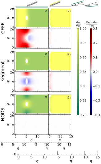
(b) $\bar{q}g_{1}g_{2}q+g$

Figure 5: Colour factor assignment and relative deviation to the squared tree-level matrix element, as in Fig. 4, for the $2\to 4+g$ configurations (a) $\bar{q}q^{\prime}\bar{q}^{\prime}q+g$ and (b) $\bar{q}g_{1}g_{2}q+g$, corresponding respectively to the Lund diagrams in Figs. 2(c) and 1(a) (with $g_{2}$ there moved to the right of $g_{1}$). The results have been obtained with the $\beta=0$ PanGlobal shower algorithm.

Next, we consider tests for $2\to 4+g$ configurations, first for $e^{+}e^{-}\to\bar{q}q^{\prime}\bar{q}^{\prime}q+g$ and then for $e^{+}e^{-}\to\bar{q}g_{1}g_{2}q+g$. A first gluon $g_{1}$ is emitted off the $\bar{q}q$ dipole with the same kinematics as in Eq. (43). The second splitting is performed with

$$\bar{q}q^{\prime}\bar{q}^{\prime}q\;{\rm configuration}:\qquad z_{\bar{q}^{\prime}}=1/4, \eta_{q^{\prime}\bar{q}^{\prime}}=10,\qquad \psi=0,$$ (44a)

$$\bar{q}g_{1}g_{2}q\;{\rm configuration}:\qquad z_{g_{2}}=10^{-16}, \eta_{g_{2}}=10,\qquad \psi=0\,.$$ (44b)

These configurations are such that the second splitting happens at a much smaller angle than the first gluon emission. For the first configuration ($g_{1}\to\bar{q}^{\prime}q^{\prime}$), we choose a $z$ fraction reflecting the absence of soft enhancements. For the second configuration (emission of $g_{2}$ from the quark, well separated in rapidity from $g_{1}$) we focus on a case where $g_{2}$ is much softer than $g_{1}$, though the conclusions are unchanged if we take $g_{1}$ and $g_{2}$ to have commensurate transverse momenta. Results are displayed in Fig. 5. They have features similar to those of Fig. 4, albeit with a richer structure.

The $\bar{q}q^{\prime}\bar{q}^{\prime}q$ case is shown in Fig. 5(a). The Lund diagram for the corresponding phase space, and expected colour assignments, was shown in Fig. 2(c). There are several possible ways for the additional gluon to cluster with the rest of the event. It is useful to organise them from a Lund-plane viewpoint. The three different possibilities correspond to the left, centre and right panels in each plot of Fig. 5(a). First, primary emissions (left-hand panel, labelled $q$) include cases where $g_{2}$ clusters with either $\bar{q}$, $q$, or the full $g_{1}(\to q^{\prime}{\bar{q}}^{\prime})q$ system, corresponding respectively to $\eta<0$ (not shown), $\eta\gtrsim 5$ and $0<\eta\lesssim 5$. Next, secondary emissions (middle panel, labelled $q^{\prime}$) include clusterings with either $q^{\prime}$ (the harder of $q^{\prime}$ and $\bar{q}^{\prime}$) or the $g_{1}\to q^{\prime}\bar{q}^{\prime}$ system. These correspond to the regions $\eta\gtrsim 10$ and $5\lesssim\eta\lesssim 10$ respectively. Finally, tertiary emissions (right-hand panel, labelled $\bar{q}^{\prime}$) correspond to clusterings of the soft gluon $g$ with $\bar{q}^{\prime}$. The hole observed in the primary (secondary) plane corresponds to the region where emissions are clustered in the secondary (tertiary) plane. The correct colour assignment involves a factor $C_{F}$ everywhere except in the region $5\lesssim\eta\lesssim 10$ of the $q^{\prime}$-labelled plot, where the emission of $g$ is sensitive to the net colour-octet charge of the whole $g_{1}\to q^{\prime}{\bar{q}}^{\prime}$ system. The CFFE method tracks neither the intermediate particles nor segments, and therefore blindly applies a factor $C_{F}$ across phase-space. Our segment and NODS schemes, in contrast, display the correct behaviour along the intermediate gluon segment. In the case of the segment method, azimuthal deviations from the exact matrix element are observed to be of similar size as shown above in Fig. 4. Note also the discontinuity in the segment-method ${\bar{q}}^{\prime}$ panel at $\eta=10$. This is a consequence of our choice to make discontinuous transitions in the segment approach. Similar features are present in the other plots, but are less immediately visible because they coincide with the phase-space boundaries between primary and secondary Lund planes.

Next, we turn to the $\bar{q}g_{1}g_{2}q$ configuration (Fig. 5(b)), where the gluons $g_{1}$ and $g_{2}$ are primary emissions, and the holes both appear on the (primary) $q$-leaf. The corresponding Lund diagram would be Fig. 1(a) with $g_{2}$ there moved to the right of $g_{1}$. In this case, the three panels correspond to primary emissions, emissions from the secondary $g_{1}$ Lund leaf and emissions from the secondary $g_{2}$ leaf. In the CFFE scheme, the region on the $q$-leaf extending from $\eta=0$ to the gluon’s position $\eta=\eta_{g_{1}}=10$, is assigned a wrong colour factor of $C_{A}/2$. For the segment and ME methods, the same region gets a correct factor of $C_{F}$. In all cases a factor of $C_{A}/2$ is correctly applied to emissions on the $g_{1}$- and $g_{2}$-leaves.

Note that the discrepancies in the CFFE approach are log-enhanced, and therefore as we discussed in section 6.1, can affect subleading-colour contributions to DL terms. For the segment method, the discrepancies are localised around the rapidities of the emission in the parent event and they are designed to integrate to zero. We will explicitly test (and confirm) this below in section 6.3.

The results in this section demonstrate that even though our segment and NODS corrections only ever consider the structure of double-emission matrix elements, their iteration reproduces the full-colour soft matrix elements for higher multiplicities, in the appropriate angular-ordered limits.

For a study of the NODS method for parent events that are not angular-ordered, see Appendix A, which shows that discrepancies do then arise relative to the correct full-colour matrix element, as is to be expected. For some configurations they reach $15\%$.

6.3 Integrated results

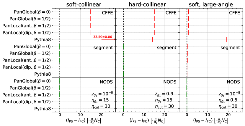
Figure 6: Normalised deviation of the integrated rate of parton-shower soft emission (from a ${\bar{q}}g_{1}q$ system), relative to analytic full-colour result, i.e. $\frac{\pi}{\alpha_{s}}N_{\text{{c}}}(I_{\text{PS}}-I_{\text{FC}})$, with $I_{\text{FC}}$ as given in Eq. (45). The results are shown for several parton showers and colour schemes for emission from a ${\bar{q}}g_{1}q$ system. The kinematics of $g_{1}$ are indicated in each column, and the integral bounds are set to $\eta_{\text{cut}}=30$. The results are colour-coded green and red, respectively, according to whether the result is consistent with zero, or not.

As noted in section 3.2, for observables such as the multiplicity, a shower that gives the correct full-colour rapidity and azimuth integral for the rate of soft emissions is expected to be correct at NDL-FC accuracy. Here we evaluate such integrals explicitly. Keeping in mind Eqs. (10) and (17), we compute the parton shower’s integrated rate of emission, $I_{\text{PS}}$, for $\bar{q}g_{1}q+g$, with the collinear cut-off set to $\eta_{\rm cut}=30$ (i.e. we integrate over the whole rapidity and azimuth phase-space, but exclude cones of half-angle corresponding to $\eta_{\rm cut}$ around each parton). Fig. 6 summarises the integral results for the CFFE, segment, and NODS colour schemes, for each of three different kinematic regimes for $g_{1}$: a soft-collinear regime, a hard-collinear regime and a soft large-angle regime (cf. values of $z_{g_{1}}$ and $\eta_{g_{1}}$ as labelled on the plots). The known full-colour result is:

$$I_{\text{FC}}=\frac{2\alpha_{s}\,\Delta\!\ln E}{\pi}\left[2C_{F}\eta_{\text{cut}}+C_{A}\left(\eta_{\text{cut}}-\eta_{g_{1}}-\ln\left(1+e^{-2\eta_{g_{1}}}\right)\right)\right],$$ (45)

which extends Eq. (10) beyond the small-angle limit for $g_{1}$ (i.e. Eq. (45) is valid for any $\eta_{g_{1}}$). The plot shows the difference between the shower result and Eq. (45), multiplied by

$$\mathcal{N}=\frac{\pi}{2\alpha_{s}}\frac{1}{C_{A}/2-C_{F}}=\frac{\pi}{\alpha_{s}}N_{\text{{c}}}\,.$$ (46)

This normalisation is chosen so that $\mathcal{N}(I_{\text{PS}}-I_{\text{FC}})$ is equivalent to the effective net extent in rapidity over which there is a $C_{A}/2$ versus $C_{F}$ discrepancy.

For soft- and hard-collinear configurations (left and middle columns), one observes a deviation in the integral computed with the CFFE scheme due to the mis-assignment of a factor $C_{A}/2$ on the $q$-leaf, see Fig. 4. The difference between the PanScales shower family and the Pythia 8 parton shower is explained by the different separation of dipole elements mentioned in section 5. In comparison, the segment and NODS colour schemes reproduce the expression expected from angular ordering for all the parton showers we considered.

The last configuration that we examine is when $g_{1}$ is soft and at large angles (rightmost column of Fig. 6). In the case of the CFFE scheme, there remains a disagreement for all parton showers, although it is again smaller for the PanScales family than for Pythia 8.

Interestingly, the segment method also shows a residual deviation from the analytic expression. This expected deviation stems from our use of the small-angle limit to determine transition points between segments also in the large-angle region. It can be calculated explicitly for PanScales showers following the same procedure as in section 3.2 for arbitrary values of $\theta_{g_{1}q}$:

$$I_{\text{PS}}^{(\text{segment})}-I_{\text{FC}}=\frac{\alpha_{s}}{\pi}\left(C_{A}-2C_{F}\right)\left\{\begin{array}[]{lll}\eta_{g_{1}}+\ln(1+e^{-2\eta_{g_{1}}}),&&|\eta_{g_{1}}|<\eta_{t},\\ \frac{3}{2}\ln(1+e^{-2|\eta_{g_{1}}\!|}),&&|\eta_{g_{1}}|>\eta_{t},\end{array}\right.$$ (47)

where $\eta_{t}=\frac{1}{2}\ln\frac{1+\sqrt{5}}{2}\simeq 0.241$ solves $\eta_{t}=\frac{1}{2}\ln(1+e^{-2\eta_{t}})$. The fact that Eq. (47) is of order $\alpha_{s}/N_{\text{{c}}}$ for $\eta_{g_{1}}$ close to zero, together with its exponential decrease as $\eta_{g_{1}}$ increases, ensures that its impact on observables such as the multiplicity is NNDL-NLC.

As expected, the NODS scheme reproduces the full-colour analytic integral even when $g_{1}$ is at large angles.

7 Numerical tests for observables

In this section, we follow the approach proposed in Ref. Dasgupta:2020fwr for testing the logarithmic structure of showers with specific observables in $e^{+}e^{-}$ collisions. Such tests implicitly probe virtual as well as real corrections and so provide a powerful verification of the correct overall assembly of the different shower elements. As the reader will recall from the introduction, the tests can be separated into two broad classes, according to whether one is probing a double-logarithmic structure (DL, NDL, etc.) or an exponentiated (LL, NLL, etc.) structure. We start by outlining the structure of the tests, keeping in mind that we will adjust the details for each specific observable.

For the double-logarithmic case, Eq. (2), when we study some event variable $V(\alpha_{s},L)$, we will fix

$$\xi=\alpha_{s}L^{2}\,,$$ (48)

and examine the behaviour of $V(\alpha_{s},L)$ in the limit $\alpha_{s}\to 0$ (with $L$ scaling as $-1/\sqrt{\alpha_{s}}$). For example to test N^kDL accuracy we will study a quantity such as

$$\delta V_{\text{N${}^{k}$DL}}=\lim_{\alpha_{s}\to 0}\left(\frac{V_{\text{PS}}(\alpha_{s},-\sqrt{\xi/\alpha_{s}})-V_{\text{N${}^{k}$DL}}(\alpha_{s},-\sqrt{\xi/\alpha_{s}})}{\alpha_{s}^{k/2}}\right),$$ (49)

where $V_{\text{N${}^{k}$DL}}$ is the known N^kDL prediction from resummation and $V_{\text{PS}}$ is the result from the parton shower. For a parton shower that is correct to N^kDL accuracy, $\delta V_{\text{N${}^{k}$DL}}$ should be zero. Values of $\xi$ for different momentum ranges are shown in table 1. In practice we will often use $\xi=\alpha_{s}L^{2}=5$, which is towards the upper end of the phenomenologically relevant combinations of $\alpha_{s}$ and $L$ accessible at the LHC. We perform such studies for multiplicities (section 7.1) and event shapes (section 7.2.1).

$Q$ [GeV]	$\alpha_{s}(Q)$	$p_{t,\min}$ [GeV]	$\xi=\alpha_{s}L^{2}$	$\lambda=\alpha_{s}L$	$\tau$
$91.2$	$0.1181$	$1.0$	$2.4$	$-0.53$	$0.27$
$91.2$	$0.1181$	$3.0$	$1.4$	$-0.40$	$0.18$
$91.2$	$0.1181$	$5.0$	$1.0$	$-0.34$	$0.14$
$1000$	$0.0886$	$1.0$	$4.2$	$-0.61$	$0.36$
$1000$	$0.0886$	$3.0$	$3.0$	$-0.51$	$0.26$
$1000$	$0.0886$	$5.0$	$2.5$	$-0.47$	$0.22$
$4000$	$0.0777$	$1.0$	$5.3$	$-0.64$	$0.40$
$4000$	$0.0777$	$3.0$	$4.0$	$-0.56$	$0.30$
$4000$	$0.0777$	$5.0$	$3.5$	$-0.52$	$0.26$
$20000$	$0.0680$	$1.0$	$6.7$	$-0.67$	$0.45$
$20000$	$0.0680$	$3.0$	$5.3$	$-0.60$	$0.34$
$20000$	$0.0680$	$5.0$	$4.7$	$-0.56$	$0.30$

Table 1: Values of $\xi=\alpha_{s}L^{2}$, $\lambda=\alpha_{s}L$ and $\tau$ (defined in Eq. (57)) for various upper ($Q$) and lower ($p_{t,\min}$) momentum scales. The coupling itself is in a 5-loop variable flavour number scheme Chetyrkin:2005ia ; Baikov:2016tgj ; Luthe:2016ima ; Herzog:2017ohr , while $\tau$ is evaluated for 1-loop evolution with $n_{f}=5$.

For observables whose logarithmic prediction exponentiates, Eq. (1), we can study $\ln V(\alpha_{s},L)$, taking the limit of $\alpha_{s}\to 0$ with fixed

$$\lambda=\alpha_{s}L\,.$$ (50)

To test N^kLL accuracy we can examine

$$\delta\ln V_{\text{N${}^{k}$LL}}=\lim_{\alpha_{s}\to 0}\left(\frac{\ln V_{\text{PS}}(\alpha_{s},\lambda/\alpha_{s})-\ln V_{\text{N${}^{k}$LL}}(\alpha_{s},\lambda/\alpha_{s})}{\alpha_{s}^{k-1}}\right),$$ (51)

where $V_{\text{N${}^{k}$LL}}$ is the known N^kLL prediction from resummation. For a shower that is correct to N^kLL accuracy, $\delta\ln V_{\text{N${}^{k}$LL}}$ should be zero. For a shower that is incorrect at LL accuracy, the unnormalised difference between $\ln V_{\text{PS}}$ and $\ln V_{\text{LL}}$ diverges for $\alpha_{s}\to 0$, hence Eq. (51) multiplies that difference by $\alpha_{s}$ to give a finite, non-zero result. In practice we will often use $\lambda=\alpha_{s}L=-0.5$. This corresponds to a slightly narrower range of logarithm than our choice for $\xi$, in part to help mitigate some of the technical difficulties of the $\alpha_{s}\to 0$ limit. We perform such studies for event shapes (section 7.2.2) and non-global logarithms (section 7.3).

Generation with very small $\alpha_{s}$ and fixed $\xi$ or $\lambda$ is often difficult. Many of the techniques that we use were outlined in the supplemental material to Ref. Dasgupta:2020fwr . For the work presented here we added three main new advances:

1. We implemented a weighted generation technique that is equivalent to evolving multiple replicas of an event, discarding a replica when it emits into a region of phase-space that we wish to veto, and then adjusting the number of replicas and their weights so as to continue generating with the original effective number of replicas (cf. section 3 of Ref. Lonnblad:2012hz ). For the combinations of $\alpha_{s}$, shower and event-shape that were most challenging in Ref. Dasgupta:2020fwr , this enabled us to save about an order of magnitude in computing time, associated with accessing regions with very strong Sudakov suppression. It also enabled us to reach small $\alpha_{s}$ values that were simply not feasible in Ref. Dasgupta:2020fwr , facilitating the extrapolation to $\alpha_{s}=0$.

2. We adjusted the shower implementation so that it can track differences in directions between neighbouring particles in the dipole chain. This works around issues that arise in normal shower implementations where it becomes difficult to determine angles between particles (and dot products, etc.) when those angles go below machine precision $\epsilon$. This, together with the next point, was especially useful in allowing for smaller $\alpha_{s}$ and larger values of the (absolute) logarithm in double-logarithmic tests, though it also facilitated cutoff dependence tests in the NLL event-shape studies. It has a small $\sim 30\%$ speed penalty, and some implementation overhead, but avoids the need for the double-double and quad-double types hida2000quad used, with substantially larger speed penalties, in Ref. Dasgupta:2020fwr .

3. To allow for momenta across such disparate scales that the logarithm of the ratio of scales is truly large ($|L|\gtrsim\frac{1}{2}\log\mu\simeq 354$ where $\mu\simeq 1.8\times 10^{308}$ is the maximum number that can be represented in double precision), we implemented a new floating type that supplements a normal double-precision number with a 64-bit integer to store the exponent, replacing the usual 11 exponent bits in a double precision number. This came with a speed penalty relative to double precision numbers of about $\times 4$, but was substantially faster than solutions we investigated based on the MPFR fousse2007mpfr or Boost multiprecision libraries. It was particularly valuable for double-logarithmic tests and useful also for tests of non-global observables.

Throughout we will run with the physical colour factors, $N_{\text{{c}}}=3$, $C_{F}=(N_{\text{{c}}}^{2}-1)/(2N_{\text{{c}}})=4/3$, $C_{A}=N_{\text{{c}}}$ and $n_{f}=5$ (except for leading-$N_{\text{{c}}}$ comparison results, where we use $C_{F}=\frac{1}{2}C_{A}=\frac{3}{2}$).

7.1 Particle multiplicity

One of the most powerful tests of a parton shower is its prediction for the particle or subjet multiplicity. To reproduce the NDL multiplicity requires correct modelling of a variety of aspects of a parton shower, including nested $g\to gg$ and $g\to q\bar{q}$ splittings. Ref. Dasgupta:2020fwr demonstrated agreement between a range of dipole showers and NDL-LC predictions. We expect the segment and NODS schemes of sections 3 and 4 to bring NDL-FC agreement. For example, in the segment method, the general pattern of $C_{F}$ dipole segments associated with the Born ${\bar{q}}q$ pair should guarantee DL-FC terms, while the specific choices of transition points for the segments, together with the $C_{F}$ segments for $g\to q^{\prime}{\bar{q}}^{\prime}$ splittings, should ensure NDL-FC accuracy.

Strictly speaking, the particle multiplicity is infrared and collinear (IRC) unsafe. A closely related, but IRC-safe, quantity is the subjet multiplicity Catani:1991pm in the $k_{t}$ jet algorithm Catani:1991hj . Ref. Dasgupta:2020fwr directly computed that subjet multiplicity comparing to the results of Ref. Catani:1991pm . Here we take a slightly different approach that avoids the need for jet clustering, but can still be directly compared to the results of Ref. Catani:1991pm . We run the shower as normal, but set the running coupling to zero below some threshold transverse momentum $k_{t,\text{cut}}$. At NDL accuracy, the multiplicity with such a procedure should be identical to that with a clustering threshold for the subjets of $y_{\text{cut}}=k_{t,\text{cut}}^{2}/Q^{2}$. Only starting from NNDL do we expect differences to arise between the multiplicity for a shower definition of a $k_{t}$ cutoff and the $k_{t}$ algorithm definition. We have explicitly verified that this is the case at leading colour.

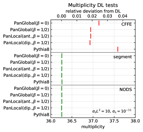
Figure 7: DL shower multiplicity tests, showing results for the parton multiplicity at $\xi=\alpha_{s}L^{2}=5$ in various parton showers and colour schemes, for a sufficiently small value of $\alpha_{s}$ that NDL terms can be neglected. The DL expectation from Eq. (52) is $N_{\text{DL}}\simeq 10.9008$.

The analytic expression for the multiplicity in $e^{+}e^{-}\to q{\bar{q}}$ events, up to and including NDL terms, can be straightforwardly extracted from Ref. Catani:1991pm ,

$$N =2\frac{C_{F}}{C_{A}}\left(1+\frac{b(2B-1)}{8\pi}\sqrt{\alpha_{s}\xi}\right)\cosh\left(\sqrt{\frac{2C_{A}}{\pi}\xi}\right)+2\left(1-\frac{C_{F}}{C_{A}}\right)\left(1+\frac{n_{f}C_{F}}{16\pi C_{A}}\sqrt{\alpha_{s}\xi}\right)$$

$$+\sqrt{\frac{\alpha_{s}\xi}{32\pi C_{A}}}\frac{2C_{F}}{C_{A}}\left[6C_{A}+\left(\frac{5}{2}-3B-\frac{C_{A}\xi}{\pi}\right)b\right]\sinh\left(\sqrt{\frac{2C_{A}}{\pi}\xi}\right),$$ (52)

in the approximation that $|L|\gg 1$, with $b=\frac{11C_{A}-2n_{f}}{3}$ and $B=1+\frac{8n_{f}(C_{A}-C_{F})}{3bC_{A}}$. Fig. 7 shows the multiplicity $N$ for $\xi=5$ at a value of $\alpha_{s}=5\times 10^{{-}12}$, which is sufficiently tiny that one can neglect subleading corrections to within an accuracy of $\sqrt{\alpha_{s}}\simeq 2.24\times 10^{{-}6}$. The figure compares several shower algorithms (the main PanScales showers and our implementation of the Pythia 8 shower), and three colour schemes, with the analytic DL result. We see that the CFFE scheme, the default in many showers including Pythia 8, differs by up to $\sim 3\%$ from the analytic result. A $3\%$ difference is not a huge effect, but it remains a subleading-$N_{\text{{c}}}$ DL difference and gives a measure of the practical impact of such contributions, i.e. $\sim 1/(3N_{\text{{c}}}^{2})$. For comparison, the differential matrix element plots, Figs. 4 and 5, showed $\sim 10\%$ differences for the CFFE approach in extended phase-space regions. Our new segment and NODS approaches coincide well with the DL analytic multiplicity result for all showers, including when applied to the Pythia 8 shower.

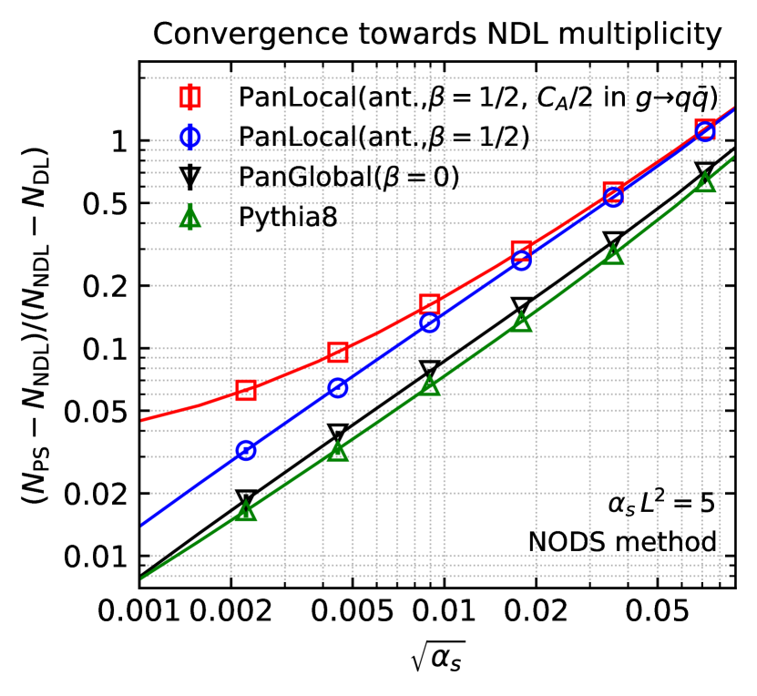
(a)

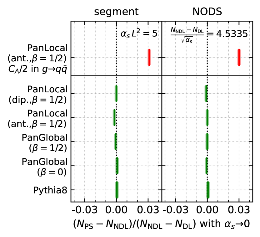
(b)

Figure 8: NDL shower multiplicity tests. (a) Results for $\frac{N_{\text{PS}}-N_{\text{NDL}}}{N_{\text{NDL}}-N_{\text{DL}}}$, for a variety of parton showers in the NODS colour scheme, as a function of $\sqrt{\alpha_{s}}$, showing that they vanish as $\alpha_{s}\to 0$, as required to achieve full-colour NDL accuracy. The curves depict a fit that is a polynomial in powers of $\sqrt{\alpha_{s}}$. (b) Explicit extrapolation of $\frac{N_{\text{PS}}-N_{\text{NDL}}}{N_{\text{NDL}}-N_{\text{DL}}}$ to $\alpha_{s}=0$, for a range of showers, with the segment and NODS colour schemes. In both plots we also illustrate the NDL-level discrepancy that arises in a scheme where quarks from $g\to q\bar{q}$ splittings erroneously continue to emit with a $C_{A}/2$ colour factor.

To test the NDL multiplicity terms, we need to examine $\delta N_{\text{NDL}}$, as defined in Eq. (49). For this comparison, we need $\alpha_{s}$ to be large enough for $\sqrt{\alpha_{s}}$ terms in the multiplicity to be visible after summing over a finite number of Monte Carlo events, while also small enough that we can safely extrapolate away ${\cal O}\left(\alpha_{s}\right)$ terms. To this end, Fig. 8(a) shows

$$\frac{N_{\text{PS}}-N_{\text{NDL}}}{N_{\text{NDL}}-N_{\text{DL}}}=\frac{N_{\text{PS}}-N_{\text{DL}}}{N_{\text{NDL}}-N_{\text{DL}}}-1,$$ (53)

a quantity conceptually similar to $\delta N_{\text{NDL}}$ in Eq. (49) (since $N_{\text{NDL}}-N_{\text{DL}}\propto\sqrt{\alpha_{s}}$), as a function of $\sqrt{\alpha_{s}}$. It shows results for the NODS method for several showers and one sees that most of the results go to zero as $\alpha_{s}\to 0$, with the exception of the red curve, to which we return below (the segment method, not shown, gives almost identical results). The result of the actual $\alpha_{s}\to 0$ extrapolation (using a cubic polynomial extrapolation based on $\alpha_{s}=\{0.000005,0.00032,0.00128,0.00512\}$) is shown in Fig. 8(b) for each shower and for each of the segment and NODS methods. All results are consistent with the (full-colour) NDL result, to within the small statistical errors.

Fig. 8 also includes results (red points) obtained using a deliberately erroneous prescription that omits the insertion of new $C_{F}$ segments following $g\to q\bar{q}$ branchings, resulting in those quarks emitting with a $C_{A}/2$ colour factor. While this prescription gives the correct DL-FC result, one should expect it to fail to reproduce the NDL-FC results, because $g\to q{\bar{q}}$ splittings start to contribute to the multiplicity from NDL terms onwards, as can be verified by inspecting the $n_{f}$ terms in Eq. (52). We see in Fig. 8(a) that with this incorrect treatment of $g\to q\bar{q}$ splittings, the limit $\sqrt{\alpha_{s}}\to 0$ fails to converge to the NDL expectation. Instead the extrapolated NDL coefficient is $\sim 3\%$ larger than the analytic expectation.

We have also carried out similar tests for the multiplicity in $H\to gg$ events for all showers shown in Fig. 8 and found a similar level of agreement with the full-colour NDL predictions for both the segment and NODS colour prescriptions.

7.2 Event shapes

The main event shapes that we consider here are obtained by considering all primary Lund declusterings Dreyer:2018nbf , and for each declustering evaluating,

$$u_{i}^{\beta_{\text{obs}}}\equiv\frac{k_{ti}e^{-\beta_{\text{obs}}|\eta_{i}|}}{Q},$$ (54)

where $k_{ti}$ is the transverse momentum of the declustered subjet $i$ with respect to its partner direction, and $\eta_{i}=\ln\tan\theta_{i}/2$, with $\theta_{i}$ the angle of the declustered subjet with respect to the partner. The parameter $\beta_{\text{obs}}$ determines the relative weighting of different rapidities and we will consider three values, $\beta_{\text{obs}}=0,\frac{1}{2},1$. We will study two combinations of the $u_{i}$,

$$M_{\beta_{\text{obs}}}\equiv\max_{i}\left\{u_{i}^{\beta_{\text{obs}}}\right\}\,,\qquad S_{\beta_{\text{obs}}}\equiv\sum_{i}u_{i}^{\beta_{\text{obs}}}\,.$$ (55)

For each event shape, we define $\Sigma(\alpha_{s},L)$ to be the fraction of events for which that event shape has a value smaller than a threshold defined to be $e^{-|L|}$. Up to NLL accuracy, $\Sigma(\alpha_{s},L)$ for $M_{\beta_{\text{obs}}=0}$ coincides with that for the Cambridge $\sqrt{y_{23}}$ resolution scale Dokshitzer:1997in , and $S_{\beta_{\text{obs}}=1}$ with that for one minus the thrust (below, in section 7.2.2, we will consider those explicitly as well).

Ref. Dasgupta:2018nvj showed that the CFFE procedure led to spurious subleading-$N_{\text{{c}}}$ terms starting from order $\alpha_{s}^{2}L^{4}$ in standard dipole showers. With similar reasoning it is straightforward to show that the issue is present also for the PanScales showers with the CFFE approach. Those issues are caused by mis-attribution of a $C_{A}/2$ colour factor to emissions that should be seen as coming from the primary ${\bar{q}}q$ pair. Once that issue is fixed, one should obtain NLL-FC accurate results for all PanScales showers that already give NLL-LC accuracy.

Given that the CFFE issue arises at order $\alpha_{s}^{2}L^{4}$, one expects to be able to observe it numerically in both DL and LL-style tests. As we shall see below, numerical LL and NLL tests require us to prune the shower branchings, so as to keep multiplicities under control in the limit $\alpha_{s}\to 0$ for fixed $\lambda=\alpha_{s}L$. That pruning can be delicate in situations with DL discrepancies. Accordingly we first carry out DL tests, for which we can run complete, unpruned showers.

When it helps to limit notational ambiguity with respect to $\beta_{\text{obs}}$, in some cases below we will write $\beta_{\text{PS}}$ instead of $\beta$ for the parameter that determines the shower ordering variable (cf. Eq. (13)).

7.2.1 Double-logarithmic study

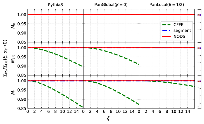
Figure 9: Double-logarithmic tests for event shapes, showing the ratio $\Sigma_{\text{PS}}/\Sigma_{\text{DL}}$ in the limit of $\alpha_{s}\to 0$ for fixed $\xi=\alpha_{s}\ln^{2}M_{\beta_{\text{obs}}}$, as a function of $\xi$. The $M_{\beta_{\text{obs}}}$ observables are defined in Eq. (55), with $M_{0}$ equivalent to the Cambridge $y_{3}$ clustering scale, and $M_{1}$ similar to the thrust at DL accuracy. Each row shows a different parton-shower algorithm, each column a different colour scheme, and each subplot shows results for three values of $\beta_{\text{obs}}$. Showers that are DL-FC accurate give a ratio of $1$ for all $\xi$. The CFFE scheme shows DL discrepancies for at least some of the observables for each shower. The segment and NODS schemes agree with the DL-FC expectation.

To enable us to study the subleading colour double-logarithmic contributions, Fig. 9 shows $\Sigma_{\text{PS}}/\Sigma_{\text{DL}}$ as a function of $\xi=\alpha_{s}L^{2}$, in the limit of $\alpha_{s}\to 0$, for $M_{\beta_{\text{obs}}}$ observables with three different values of $\beta_{\text{obs}}$. It includes results for two PanScales showers and for Pythia 8, for all three colour schemes. To understand the plots, it is useful to recall that the PanScales showers are ordered in a variable $\sim k_{t}e^{-\beta_{\text{PS}}|\eta|}$ (we show PanGlobal with $\beta_{\text{PS}}=0$ and PanLocal with $\beta_{\text{PS}}=1/2$). We expect (and see) that double logarithmic discrepancies are present in the CFFE scheme for any $\beta_{\text{obs}}>\beta_{\text{PS}}$. For Pythia 8, which is $k_{t}$ ordered, we expect DL discrepancies to be present in the CFFE scheme for any $\beta_{\text{obs}}\neq 0$, though our tests only consider $\beta_{\text{obs}}\geq 0$. Discrepancies at DL accuracy are clearly visible as deviations of the curves from $1$. In the physically accessible region, $\xi\lesssim 7$, those discrepancies are fairly modest, no more than $2{-}3$ percent. The results for the segment and NODS colour scheme are all consistent with $1$. While shown only for a subset of showers and for the $M_{\beta_{\text{obs}}}$ observables, the results for other PanScales showers are the same for any given $\beta_{\text{PS}}$ and for the $S_{\beta_{\text{obs}}}$ observables.

In the case of the PanScales showers, one can also calculate the analytic form of the CFFE discrepancies, cf. Appendix B. The analytic results agree well with the observed shower discrepancies. It is interesting to consider the large-$\xi$ limit of the discrepancy, which will be relevant also in understanding the results of the next subsection. For example, for the thrust determined with any of the PanScales showers with $\beta_{\text{PS}}=0$, we find that

$$\lim_{\xi\to\infty}\lim_{\alpha_{s}\to 0}\frac{\ln\Sigma_{\beta_{\text{PS}}=0}(\alpha_{s},-\sqrt{\xi/\alpha_{s}})}{\ln\Sigma_{DL}(\alpha_{s},-\sqrt{\xi/\alpha_{s}})}=1+\frac{1}{2N_{\text{{c}}}^{2}-1}\,.$$ (56)

However, the approach to this limit is very slow: for $\xi=5$ the ratio is about $1.009$, to be compared to an asymptotic value of $1+1/17\simeq 1.0588$.

7.2.2 LL and NLL studies

Our next set of tests is to carry out LL and NLL studies for the same set of event shapes discussed above, supplemented with the total and wide-jet broadenings ($B_{T},B_{W}$) Catani:1992jc , the Cambridge $y_{23}$ jet resolution parameter Dokshitzer:1997in , thrust Farhi:1977sg and fractional energy-energy correlation moments ($\text{FC}_{x}$) Banfi:2004yd . We consider the limit $\alpha_{s}\to 0$ for fixed $\lambda=\alpha_{s}L$.

A fundamental difficulty with these LL and NLL studies is that the logarithm of the multiplicity, $\ln N$, scales as $\sqrt{\alpha_{s}L^{2}}$, cf. Eq. (52), and when we fix $\lambda=\alpha_{s}L$ and take the limit $\alpha_{s}\to 0$, the logarithm of the multiplicity blows up as $\sqrt{1/\alpha_{s}}$. Since generation time and memory consumption scale at least in proportion to $N$, event generation becomes prohibitively expensive with too small a value of $\alpha_{s}$.

To address this problem we adopt a strategy where, at each stage of the shower, branchings that are guaranteed to be irrelevant to the observable are vetoed. Specifically, for a given $\beta_{\text{obs}}$, we track the maximum value of $O_{\text{approx}}=k_{t,\text{approx}}e^{-\beta_{\text{obs}}|\eta_{\text{approx}}|}$ that has occurred so far in the showering of the event (using Eq. (14) for $\eta_{\text{approx}}$ and $k_{t,\text{approx}}$ equivalent to the $k_{t}$ in Eq. (13)). We accept a given new branching only if it has $O_{\text{approx}}>e^{-\Delta}O_{\text{approx,max}}$, with $\Delta$ a parameter to be chosen appropriately. The logarithm of the multiplicity is then expected to scale roughly as $\sqrt{\alpha_{s}\Delta^{2}}+\ln|\lambda\Delta|$. The value of $\Delta$ should be small enough that the multiplicity remains under control, and large enough that recursively IRC safe observables Banfi:2004yd are not affected by it, which is ensured by the requirement $e^{-\Delta}\ll 1$.

For shower–observable combinations where there is a double-logarithmic subleading-$N_{\text{{c}}}$ effect, we also need to be aware that the mechanism generating that effect may only be fully operational if $\alpha_{s}\Delta^{2}\gg 1$, which is in tension with the constraint on the multiplicity. In practice it is difficult to ensure that the full DL discrepancy is captured in LL tests, especially when considering the interplay between the $\alpha_{s}\to 0$ and $\Delta\to\infty$ limits. Our approach will instead be to ensure that the combinations of $\alpha_{s}$ and $\Delta$ are such that the presence of any DL issues is correctly diagnosed in our LL tests, even if we do not reproduce the exact value of any discrepancy.

This is illustrated in Fig. 10, which shows LL tests for the CFFE colour approach, using $\Delta=18$ and a quadratic polynomial extrapolation to $\alpha_{s}=0$ based on runs at $\alpha_{s}=\{0.0025,0.005,0.01\}$. There, one clearly sees that the set of shower–observable combinations that fails the LL test is consistent with the expectations from the DL tests in Fig. 9 and from Appendix B. However, taking the example of the $\beta_{\text{obs}}=1$ observables, for the PanGlobal shower with $\beta_{\text{PS}}=0$, one sees a discrepancy of $0.056$, to be compared to the expectation of $0.068$ in table 2 of Appendix B, as obtained when one first takes the limit $\Delta\to\infty$, and then $\alpha_{s}\to 0$ (this $0.068$ is the running coupling analogue of Eq. (56)).

Figure 10: LL test of the CFFE scheme for event shapes, showing the expected pattern of discrepancies for the PanScales and Pythia 8 showers. For further details, see text.

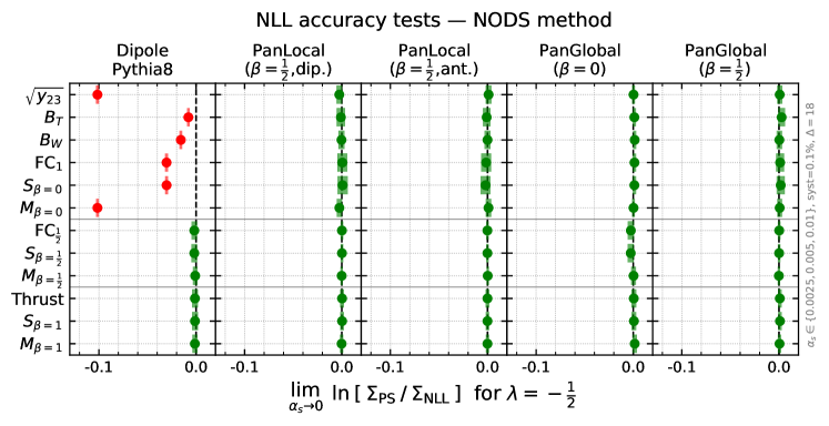
Figure 11: NLL global event-shape tests of the segment and NODS colour schemes, showing NLL agreement for $\beta=1/2$ PanScales showers and for the $\beta=0$ PanGlobal shower. In contrast to the NLL-LC tests of Ref. Dasgupta:2020fwr , the Pythia 8 $\beta_{\text{obs}}>0$ results here are coloured green rather than amber, because our colour code does not incorporate the information about failure of exponentiation in fixed-order tests, tests that we have not explicitly repeated for this paper.

The LL tests for the segment and NODS colour schemes (not shown in Fig. 10) are consistent with the analytic LL results for all observables and showers, including Pythia 8. Accordingly in Fig. 11, where we show the full-colour NLL tests, i.e. examining $\delta\ln\Sigma_{\text{NLL}}$, Eq. (51), we include results just for those two schemes. For all showers that were in agreement with NLL predictions at NLL-LC in Ref. Dasgupta:2020fwr , we now see that these two new colour schemes ensure agreement with the NLL-FC predictions. This is to be expected, because, beyond the recoil issues that were relevant for NLL-LC accuracy, NLL-FC requires the correct treatment of the colour factor only for emissions that are widely separated in rapidity, which the segment and NODS schemes both accomplish by design.

Note that we have only tested event-shape observables that vanish in the $2$-jet limit. One could also envisage testing event shapes such as the thrust minor and $D$-parameter, which vanish in the limit of 3 narrow jets, and whose NLL-FC resummations have long been known Banfi:2000si ; Banfi:2001pb for planar events. Our expectation is that the NODS scheme (but not the segment scheme) will yield the correct NLL-FC results also for these observables, as long as the appropriate matching is included for the 3-jet matrix element, and the segment variables and auxiliary momenta are properly initialised.

7.3 Energy flow in a rapidity slice

The final observable that we consider is the probability, $\Sigma(\alpha_{s},L)$, for the energy in a given central slice of rapidity to be less than $e^{-|L|}Q$. Such an observable is of interest because its resummation involves non-global logarithms, single-logarithmic terms $\alpha_{s}^{n}L^{n}$ that involve configurations with an arbitrary number of (soft, large-angle) gluons in the neighbourhood of the slice Dasgupta:2001sh ; Dasgupta:2002bw (see also Ref. Banfi:2002hw ). The full-colour resummation for such observables is sensitive to arbitrarily complex colour correlators, both in the real emissions and the virtual corrections, which need to be evaluated at amplitude level. The resulting subleading-colour single-logarithmic corrections go far beyond the scope of the colour schemes that we introduced in sections 3 and 4. In particular, we expect the segment scheme to be correct at full colour only up to order $\alpha_{s}L$, and the NODS scheme to be correct at full colour up to order $\alpha_{s}^{2}L^{2}$. Recall that leading-colour all-order single-logarithmic accuracy for PanScales showers was demonstrated in Ref. Dasgupta:2020fwr .

The question we ask in this section is to what extent our schemes differ from a full-colour computation. Such a calculation was performed for the energy flow in a slice for the $Z\to{\bar{q}}q$ process, by Hatta and Ueda Hatta:2013iba . Their approach was based on a refinement of a proposal by Weigert Weigert:2003mm , whereby the problem was reduced to the simulation of associated Langevin dynamics in the space of Wilson lines, and solved on a two-dimensional angular grid. It was also applied, with Hagiwara, to the calculation of a hemisphere observable Hagiwara:2015bia and, very recently, to $H\to gg$ decays and a number of $2\to 2$ scattering processes Hatta:2020wre . The approach was formulated in such a way that it included only the single logarithms, $\alpha_{s}^{n}L^{n}$. Accordingly, in using it as a reference to which to compare our $\alpha_{s}\to 0$ limit, we can be sure that any difference is exclusively associated with subleading colour effects.

Two other calculations are based on parton showers at finite $\alpha_{s}$ and a truncation of the $1/N_{\text{{c}}}^{2}$ series: Nagy and Soper examined rapidity gaps between dijets at hadron colliders Nagy:2019pjp ; Nagy:2019rwb , while De Angelis, Forshaw and Plätzer examined the energy in a slice for the $Z\to{\bar{q}}q$ and $H\to gg$ processes DeAngelis:2020rvq . Only the processes examined in that latter paper are within the scope of our work here, but their simulation at finite $\alpha_{s}$ precludes a meaningful direct comparison, because it would be impossible to know whether any differences between their results and ours are associated with subleading-colour effects or instead subleading logarithmic ($\alpha_{s}^{n}L^{n-1}$) effects.

The specific definition of the energy in a rapidity slice is as follows: we cluster each event with the $e^{+}e^{-}$ Cambridge algorithm Dokshitzer:1997in with the $y_{\text{cut}}$ parameter set to $1$ and then undo one step of the resulting clustering sequence to obtain two back-to-back jets. Defining rapidity with respect to those two jet axes, we examine the total energy contained in the rapidity region $|y|<-\ln\tan\theta_{\text{cut}}/2$, with $\theta_{\text{cut}}$ setting the boundary of the slice. We will make the choice $\theta_{\text{cut}}=\pi/3$, which coincides with that of Hatta and Ueda Hatta:2013iba . As in section 7.2.2, if we carry out a full run of the shower in the $\alpha_{s}\to 0$ limit for fixed $\alpha_{s}L$, parton multiplicities will grow too large to handle. Here, we solve this problem by vetoing emissions whose rapidity with respect to the closer end of the emitting dipole is larger than $\eta_{\max}$, which by default we take to be $10$ (we will verify that reducing it to $8$ does not modify the results).

It is commonplace in studies of non-global logarithms to show the results as a function of

$$\tau(\alpha_{s},L)=\int_{Qe^{-|L|}}^{Q}\frac{dk_{t}}{k_{t}}\frac{\alpha_{s}(k_{t})}{\pi}=\int_{L}^{0}\frac{d\ell}{\pi}\frac{\alpha_{s}(Q)}{1+2b_{0}\alpha_{s}(Q)\ell}=-\frac{1}{2\pi b_{0}}\ln\left(1+2b_{0}\alpha_{s}(Q)L\right)\,,$$ (57)

with $b_{0}=\frac{11C_{A}-2n_{f}}{12\pi}$ and where the result on the right-hand side is given for a one-loop running, which is the only contribution that survives in the limit $\alpha_{s}\to 0$ at fixed $\lambda=\alpha_{s}L$. Values of $\tau$ for various momentum ranges are shown in table 1 and, at the LHC, the largest accessible value is $\tau\simeq 0.4$.

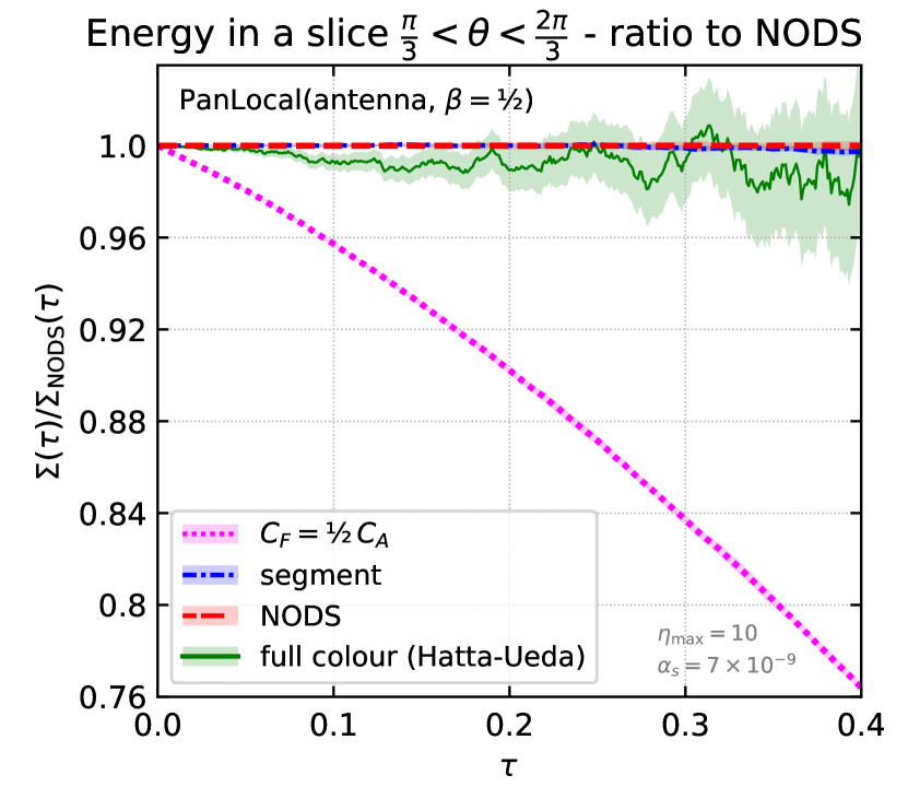
(a)

(b)

Figure 12: NLL (single-logarithmic) tests for a non-global observable. (a) Fraction of events whose energy flow in a central slice of rapidity is less than $e^{-|L|}Q$, shown in the limit $\alpha_{s}\to 0$ for fixed $\alpha_{s}L$, as a function of $\tau(\alpha_{s},L)$, defined in Eq. (57). Our results are shown for the PanScales antenna shower with $\beta_{\text{PS}}=1/2$, with three different colour schemes: leading-$N_{\text{{c}}}$ (with $C_{F}=C_{A}/2=3/2$), segment and NODS. They are compared to the full-colour Hatta-Ueda (“finite-$N_{\text{{c}}}$ (exact)”) result Hatta:2013iba . (b) Ratio of the same set of results to the NODS result, illustrating apparent consistency of the segment and NODS schemes with the Hatta-Ueda result, to within its statistical uncertainty. The agreement is potentially surprising given that our schemes do not achieve NLL-FC ($\alpha_{s}^{n}L^{n}$) accuracy for non-global observables. The thin band for our results represents the statistical uncertainty added in quadrature to estimates of systematics obtained using the difference between our default runs ($\eta_{\max}=10$ and $\alpha_{s}=0.7\times 10^{-8}$) and runs with $\eta_{\max}=8$ and $\alpha_{s}=1.4\times 10^{-8}$. Our results for other showers with the same colour schemes are very similar, as is to be expected.

Fig. 12 (left) shows the fraction of events, $\Sigma(\tau(\alpha_{s},L))$, whose energy flow in the slice is less than $e^{-|L|}Q$. It includes several results: a leading-$N_{\text{{c}}}$ result with $C_{F}=\frac{1}{2}C_{A}=3/2$, the Hatta-Ueda full-$N_{\text{{c}}}$ prediction, and our predictions with the segment and NODS methods. Recall that those methods are not expected to work beyond order $\lambda$ and $\lambda^{2}$ respectively. However in Fig. 12 (left) they are indistinguishable from the full-$N_{\text{{c}}}$ Hatta-Ueda result. To further probe this observation, the right hand plot shows ratios to a reference, which we take to be the PanLocal-antenna $\beta=1/2$ NODS (the specific choice is largely immaterial, since our aim is to compare different predictions on this ratio plot). One sees that the difference between the full-$N_{\text{{c}}}$ Hatta-Ueda result and our leading-$N_{\text{{c}}}$ result is about $23\%$ at $\tau=0.4$. Remarkably, both our segment and NODS methods seem to be in good agreement with the Hatta-Ueda result across the full range of $\tau$: the whole range is within two standard deviations of the Hatta-Ueda result, and in much of the range the agreement is within one standard deviation. Some caution is needed in interpreting these results: firstly, they correspond to one specific choice of slice size. Secondly, when using a finite-resolution angular grid (as in the Hatta-Ueda approach), there are inevitably some residual systematic effects associated with that finite resolution, and in this case we cannot exclude the possibility that they are comparable to the statistical error. A further observation is that the segment and NODS results come out largely identical, even though the former (latter) is FC-accurate only to $\alpha_{s}L$ ($\alpha_{s}^{2}L^{2}$). We attribute this to a partial cancellation that arises after azimuthal integrations. In particular, in Appendix C we demonstrate that if one breaks the azimuthal symmetry by considering a patch in azimuth and rapidity instead of a slice (which covers all azimuths), a difference between the segment and NODS scheme does appear at the statistically significant level of a couple of percent.

A final comment concerns the same slice observable for $H\to gg$ events. For a given value of $\tau$, both our segment and NODS methods are identical to the leading-$N_{\text{{c}}}$ ($2C_{F}=C_{A}=3$) result in the $\alpha_{s}\to 0$, fixed $\tau$ limit, because $g\to q\bar{q}$ branchings only affect NNLL terms, $\alpha_{s}^{n}L^{n-1}$. Subleading-$N_{\text{{c}}}$ effects start for the slice only from order $\alpha_{s}^{3}L^{3}$ onwards, because soft-gluon emission from a $ggg$ system (i.e. $\alpha_{s}^{2}L^{2}$) is given exactly by the sum of emission from three $C_{A}/2$ dipoles. Therefore we have the same formal subleading-$N_{\text{{c}}}$ accuracy as the NODS method for $Z\to q\bar{q}$: exact up to $\alpha_{s}^{2}L^{2}$, and only leading-$N_{\text{{c}}}$ for terms $\alpha_{s}^{3}L^{3}$ onwards.

Very recently, Hatta and Ueda have shown that an FC calculation for the slice observable in $H\to gg$ is in good agreement with the large-$N_{\text{{c}}}$ result, to within statistical errors Hatta:2020wre . The findings of Ref. DeAngelis:2020rvq appear to be consistent with this conclusion. Accordingly, the NODS and segment methods agree with the FC results for $H\to gg$, to within the precision of the predictions for the latter.

7.4 Timing assessment

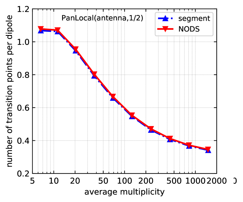
(a)

(b)

Figure 13: (a) Time per emission plotted as a function of the average multiplicity, $N$, in the event sample, for different colour schemes. To maximise the relative impact of the colour scheme timing penalty, results are shown for one of the most optimised of our shower setups, the PanLocal antenna shower with $\beta=\frac{1}{2}$, run with fixed coupling. Additional details are given in the text. (b) The average number of transition points per dipole in the segment and NODS methods, as a function of the average multiplicity.

One of the motivations behind this work is to provide a method to include logarithmically relevant subleading colour effects in parton showers that is simple and computationally efficient. In this section we show that the two methods highlighted in sections 3 and 4 bring only a modest time penalty.

To check this, we have run the PanLocal shower, in its antenna variant, setting $\beta=\frac{1}{2}$, using a fixed-coupling prescription, $\alpha_{s}=0.1$, and varying the ordering variable ($\ln v$) cut-off scale between ${-}24$ and ${-}10$. At leading-$N_{\text{{c}}}$, the PanLocal antenna shower is currently one of the fastest of our showers, and since the time penalty of the colour schemes is largely independent of the shower, the choice of PanLocal-antenna provides a worst-case estimate of the relative impact of the colour schemes. Following a similar logic, we use a fixed coupling for these tests, because our running-coupling shower implementation is not yet fully optimised, and so would produce a misleadingly high timing baseline to which to compare the timing penalties of the new colour schemes.

Fig. 13(a) shows the average event showering time divided by the average number of emissions, for each value of the $\ln v$ cutoff, plotted as a function of the average multiplicity $N$ for that $\ln v$. It includes results for four colour schemes. One sees that the timing per emission for the $C_{F}=C_{A}/2=3/2$ and CFFE schemes is about $1\mu\text{s}$, almost independently of $N$. The penalty for the segment and NODS schemes is at most $0.2\mu\text{s}$ and $0.5\mu\text{s}$ respectively. It decreases with increasing $N$, which is probably a consequence of the fact that the number of segments per dipole decreases with increasing $N$, cf. Fig. 13(b).

8 Conclusions

In this work on subleading-colour effects in final-state dipole and antenna showers, we have paid particular attention to the interplay between colour and logarithmic accuracy. Insofar as the accuracy of current parton showers is at best NLL, we argued that an essential requirement is subleading-colour accuracy for LL terms, with potentially missing subleading-$N_{\text{{c}}}$ NLL contributions being on the same footing as leading-colour NNLL terms, which are currently not available in parton showers.

In sections 3 and 4, we outlined two schemes that are simple and efficient to implement in a range of parton showers (including, e.g. the Pythia 8 shower) and that provide full-colour LL accuracy (LL-FC). One of them, the segment method, varies the colour factor along a dipole, using a Lund-diagram type classification to identify regions that should have either a $C_{F}$ or a $C_{A}/2$ colour factor, according to whether an angular-ordered picture implies emission from a quark or a gluon. The other method, dubbed NODS, nests full-colour energy-ordered double-soft matrix-element corrections for emissions from any dipole that, according to the segment approach, contains at least one $C_{F}$ segment.

In practice it was possible to engineer our approaches so as to provide full colour accuracy beyond the LL (or DL) approximation for a range of observables: all global event-shape variables, as well as observables that examine particle or jet multiplicities. For these, both of our schemes achieve NLL-FC or NDL-FC accuracy, as appropriate for the specific observable (aside from spin correlations, which do not affect the observables studied here at NLL-FC accuracy, and whose study we postpone to future work). This involved care with $g\to q\bar{q}$ splittings and with the specific locations of $C_{F}$ to $C_{A}/2$ transitions in the segment method. Numerically demonstrating the resulting accuracy relied on a range of techniques for taking the $\alpha_{s}\to 0$ limit of our showers while maintaining fixed $\alpha_{s}L$ or $\alpha_{s}L^{2}$, techniques that we have improved relative to earlier work Dasgupta:2020fwr .

The one context in which we do not achieve NLL-FC accuracy is for non-global observables (in our definition, LL for these is zero, and they start at NLL, i.e. $\alpha_{s}^{n}L^{n}$). There we achieve full-colour accuracy only for a finite set of $n$: for our segment method, $n\leq 1$, and for our NODS method, $n\leq 2$. Remarkably, despite this limitation, our schemes still give good numerical agreement with the full-colour NLL results for the energy in a slice, as obtained by Hatta and Ueda Hatta:2013iba , to within the $1{-}3\%$ statistical error of the latter. In future work, it would be interesting to gain a better understanding of why this is the case.

One of the important points related to the computational efficiency of our colour schemes, is that it makes it straightforward to obtain high statistical accuracies. The time penalty for the more sophisticated scheme, NODS, was below a microsecond per emission. That has enabled us to draw robust conclusions about non-trivial sub-leading colour effects, which were typically at the level of a few percent. This provides a target for future work on subleading colour schemes, which should straightforwardly be able to provide the high statistical precision needed to conclusively determine the size of any subleading colour effects that exist beyond those accessible in simple schemes such as those developed here.

Appendix A Matrix-element tests for non-angular ordered parent configurations

The NODS scheme is not expected to reproduce the full-colour tree-level matrix element for the emission of a gluon $g$ from configurations with two partons at commensurate angles. In this appendix we study to what extent the NODS scheme fails in such configurations, performing comparisons to the tree-level matrix element for $\bar{q}g_{1}g_{2}q+g$.

We start by emitting the first gluon $g_{1}$ from the $\bar{q}q$ dipole as in Eq. (43):

$$z_{g_{1}}=10^{-8},\quad\eta_{g_{1}}=5,\quad\psi_{g_{1}}=\pi\,.$$ (58)

We emit a second gluon $g_{2}$ close to the first gluon in rapidity, $\eta_{g_{2}}\approx\eta_{g_{1}}$. Contrary to the angular-ordered case presented in section 6.2, there are now two routes that contribute to the total rate of emission, i.e. gluon $g_{2}$ can be emitted from either of the dipoles $(\bar{q}g_{1})$ or $(g_{1}q)$. The two routes have distinct Jacobians relating the $g_{2}$ shower-generation phase-space to the Lund-diagram phase-space and this must be accounted for.

We solve numerically for the values of the generation variables $(\ln v_{2},\bar{\eta}_{2},\phi_{2})_{i}$, for each dipole $i\in\{(\bar{q}g_{1}),(g_{1}q)\}$, such that the gluon $g_{2}$ is emitted at:

$$z_{g_{2}}=10^{-16},\quad\eta_{g_{2}}=\eta_{g_{1}}+\Delta\eta_{g_{1}g_{2}},\quad\psi_{g_{2}}=0\,,$$ (59)

in the event centre-of-mass frame. We evaluate the three-dimensional Jacobian determinant

$$J_{i}=\left|\frac{\partial(\ln v_{2},\bar{\eta}_{2},\phi_{2})_{i}}{\partial(\ln E_{g_{2}},\eta_{g_{2}},\psi_{g_{2}})}\right|,$$ (60)

numerically as well. Starting from the parent configuration $\bar{q}g_{1}g_{2}q$, where $g_{2}$ has been emitted from dipole $i$, we compute the rate of emission $\sigma_{\text{PS}}^{(i)}$ of a further soft gluon $g$, and combine the contributions from the two routes weighted by their relative Jacobian factors,

$$\sigma_{\text{PS}}=\sum_{i\in\{(\bar{q}g_{1}),(g_{1}q)\}}\frac{J_{i}}{J_{(\bar{q}g_{1})}+J_{(g_{1}q)}}\sigma_{\text{PS}}^{(i)}\,.$$ (61)

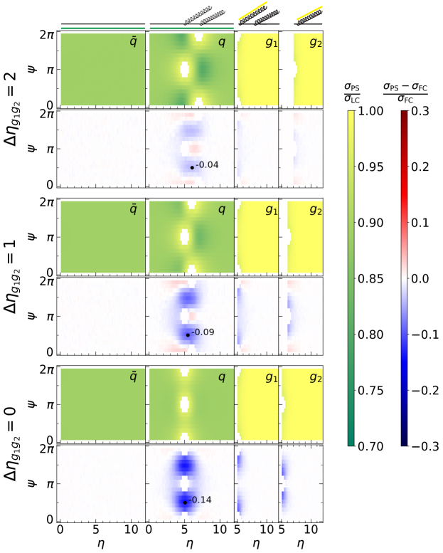
Figure 14: Results from the NODS scheme for the PanGlobal ($\beta=0$) shower, in an initial configuration $\bar{q}qg_{1}g_{2}+g$ where the two gluons $g_{1}$ and $g_{2}$ are not strongly angular-ordered. We show three configurations with the gluon $g_{2}$ brought increasingly closer to $g_{1}$: for a fixed $\eta_{g_{1}}=5$, $\psi_{g_{1}}=\pi$, the second gluon $g_{2}$ is placed at $\eta_{g_{2}}=7$ (top), $\eta_{g_{2}}=6$ (middle) and $\eta_{g_{2}}=5$ (bottom) at an azimuthal angle $\psi_{g_{2}}=0$. Black dots convey the largest negative deviation between the NODS scheme and the exact tree-level matrix element.

Results for the NODS scheme are shown in Fig. 14 for three values of the separation of $g_{1}$ and $g_{2}$ in rapidity, $\Delta\eta_{g_{1}g_{2}}=\eta_{g_{2}}-\eta_{g_{1}}=\{0,1,2\}$. The disagreement between the shower rate of emission, $\sigma_{\text{PS}}$, and the full-colour tree-level matrix element, $\sigma_{\text{FC}}$, is observed to be relatively small for $\Delta\eta_{g_{1}g_{2}}=2$, where the largest negative deviation is identified by a black dot and reaches $-4\%$ at $\psi_{g}=\pi/2$ on the $q$-leaf. As the second gluon $g_{2}$ moves to an angle close to that of the first gluon $g_{1}$, the discrepancy becomes larger, reaching a value of $-9\%$ for $\Delta\eta_{g_{1}g_{2}}=1$, and $-14\%$ for $\Delta\eta_{g_{1}g_{2}}=0$. Note that the regions where the matrix element is not reproduced are, as expected, localised around kinematic configurations for which the three emissions are at commensurate angles. These configurations are beyond the scope of the accuracy we are aiming for.

The initial 4-parton ${\bar{q}}g_{1}g_{2}q$ configurations studied here differ from the hadron-collider $2\to 2$ processes such as those studied in Ref. Hatta:2020wre , in that $g_{1}$ and $g_{2}$ are both soft. Still, our observation that non-trivial subleading-colour effects decrease as $g_{1}$ and $g_{2}$ become more separated (which is to be expected based on coherence arguments), may be relevant also more widely. Specifically, they suggest that if one seeks to maximise subleading-colour effects in hadron-collider processes, it may be of interest to consider $2\to 2$ configurations where the outgoing jets are both at the same rapidity.

Appendix B Analytical results for CFFE subleading-$N_{\text{{c}}}$ effects in event shapes

Here, we develop a (semi-)analytical approach to determining the expected DL and LL deviations in event shapes for the CFFE colour scheme as applied to the PanScales family of showers. The intent is to help provide an independent validation and understanding of some of the numerical results shown in section 7.2. The analysis is common to all of the PanLocal-dipole, PanLocal-antenna and PanGlobal showers. In contrast traditional dipole showers such as Pythia 8 are, we believe, more complex to analyse and, as can be seen from Fig. 9, they clearly yield different CFFE DL results.

Let us consider an observable with $\beta_{\text{obs}}>\beta_{\text{PS}}$ and compute $\Sigma_{\text{PS}}(L)$. Whenever we have an emission at a scale $x=\ln v$ and rapidity $\eta$, say with $\eta>0$, s.t. $x-\beta_{\text{obs}}\eta<L$, subsequent emissions (real or virtual) at rapidities between 0 and $\eta$ will have a factor $C_{A}/2$ instead of $C_{F}$. This gives the following expression

$$\frac{\Sigma_{\text{PS}}}{\Sigma_{\text{FC}}}=\left[e^{-C_{F}r_{\text{out}}(L)}+\int_{L}^{\frac{1+\beta_{\text{PS}}}{1+\beta_{\text{obs}}}L}dx\,C_{F}\,r_{\text{out}}^{\prime}(x)e^{-C_{F}r_{\text{out}}(x)-\left(\frac{C_{A}}{2}-C_{F}\right)r_{\text{in}}(x)}\right]^{2},$$ (62)

where the $r_{\text{in}}$ and $r_{\text{out}}$ Sudakov exponents correspond to the light blue and pink regions in Fig. 15, respectively. When writing this expression, the second term describes the case where the first emission below the observable boundary is at a scale $\ln v=x$. Compared to the expected result, one gets a veto for emissions below the boundary with $\ln v>x$ — the $r_{\text{out}}$ contribution — as well as a change $C_{F}\to\frac{C_{A}}{2}$ in the region corresponding to $r_{\text{in}}$. (The $r_{\text{out}}^{\prime}$ factor is minus the derivative of $r_{\text{out}}$ with respect to $x$.) The first term in the square bracket describes the situation where there is no emission below the observable boundary that affects the observable Sudakov. Finally, the overall square accounts for both hemispheres.

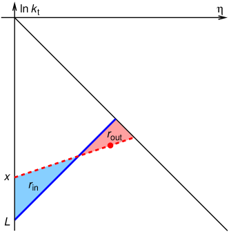
Figure 15: Primary Lund plane representation of the configuration represented in Eq. (62), with the solid line corresponding to a fixed limit $e^{-|L|}$ for the observable value and the dashed-line to a fixed value of the shower ordering variable. The emission indicated with a red dot has no direct impact on $\Sigma(\alpha_{s},L)$, but for PanScales showers with the CFFE scheme, it changes the colour factor (from $C_{F}$ to $C_{A}/2$) for all subsequent primary emissions at smaller (positive) rapidities and lower values of the shower ordering variable. This effectively modifies the Sudakov for $\Sigma(\alpha_{s},L)$ in the region shaded in blue.

The exponents $r_{\text{in}}$ and $r_{\text{out}}$ can be easily computed including one-loop running coupling effects. Here we just give their fixed-coupling expressions:

$$r_{\text{out}}(x) \overset{\text{f.c.}}{=}\frac{\alpha_{s}}{\pi}\frac{(1+\beta_{\text{obs}})(1+\beta_{\text{PS}})}{\beta_{\text{obs}}-\beta_{\text{PS}}}\left(\frac{x}{1+\beta_{\text{PS}}}-\frac{L}{1+\beta_{\text{obs}}}\right)^{2},$$ (63a)

$$r_{\text{in}}(x) \overset{\text{f.c.}}{=}\frac{\alpha_{s}}{\pi}\frac{(L-x)^{2}}{\beta_{\text{obs}}-\beta_{\text{PS}}}.$$ (63b)

From Eq. (62), we can consider two interesting limits. The first one corresponds to the study of DL in section 7.2.1, where we fixed $\xi=\alpha_{s}L^{2}$ and take the limit $\alpha_{s}\to 0$. In this case, running-coupling effects in $r_{\text{in}}$ and $r_{\text{out}}$ can be neglected as they only bring corrections proportional to $\alpha_{s}L=-\sqrt{\alpha_{s}\xi}\to 0$. In this case, Eq. (62) can be computed exactly and one finds

$$\frac{\Sigma_{\text{PS}}}{\Sigma_{\text{FC}}}\overset{\text{fixed }\xi}{\underset{\alpha_{s}\to 0}{=}}\Phi^{2},$$ (64)

with

$$\Phi =e^{-\frac{C_{F}}{\pi}\frac{\beta_{\text{obs}}-\beta_{\text{PS}}}{(1+\beta_{\text{obs}})(1+\beta_{\text{PS}})}\xi}+e^{-\frac{C_{F}}{\pi}\frac{(c-1)(\beta_{\text{obs}}-\beta_{\text{PS}})}{(1+\beta_{\text{obs}})(\beta_{\text{obs}}+(c-1)\beta_{\text{PS}}+c)}\xi}$$ (65)

$$\left[\Psi\left(-\sqrt{\frac{(1+\beta_{\text{PS}})(\beta_{\text{obs}}-\beta_{\text{PS}})(c-1)^{2}}{(\beta_{\text{obs}}+(c-1)\beta_{\text{PS}}+c)(1+\beta_{\text{obs}})^{2}}}\right)-\Psi\left(\sqrt{\frac{(\beta_{\text{obs}}-\beta_{\text{PS}})}{(1+\beta_{\text{PS}})(\beta_{\text{obs}}+(c-1)\beta_{\text{PS}}+c)}}\right)\right],$$

$c=C_{A}/(2C_{F})$, and

$$\Psi(z)=\frac{1+\beta_{\text{obs}}}{\beta_{\text{obs}}+(c-1)\beta_{\text{PS}}+c}e^{-\frac{C_{F}}{\pi}z^{2}\xi}-(c-1)\frac{\sqrt{C_{F}(\beta_{\text{obs}}-\beta_{\text{PS}})(1+\beta_{\text{PS}})\xi}}{(\beta_{\text{obs}}+(c-1)\beta_{\text{PS}}+c)^{3/2}}\text{erf}\left(\sqrt{\frac{C_{F}\xi}{\pi}}z\right).$$ (66)

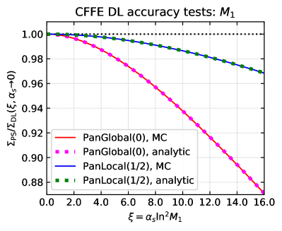
Figure 16: Demonstration that our analytical calculation of the DL discrepancy for the CFFE colour scheme, Eq. (64), agrees with the full shower runs in the $\alpha_{s}\to 0$ limit, as a function of $\xi=\alpha_{s}L^{2}$, showing the $M_{1/2}$ (left) and $M_{1}$ (right) observables.

Eq. (64) and the numerical results from section 7.2.1 are compared in Fig. 16, illustrating the perfect agreement between the two.

		$\ln\Sigma_{\text{PS}}/\ln\Sigma_{\text{FC}}-1$
$\beta_{\text{PS}}$	$\beta_{\text{obs}}$	running coupling ($\lambda=-0.5$)	fixed coupling
0	1/2	0.04749	0.03846
0	1	0.06832	0.05882
1/2	1	0.03590	0.02857

Table 2: Value of the LL discrepancy for $\alpha_{s}\to 0$ with fixed $\lambda=\alpha_{s}L=-0.5$ for various shower–observable combinations in the CFFE colour scheme.

The next limit we want to study is the one where we keep $\lambda=\alpha_{s}L$ fixed and take $\alpha_{s}\to 0$, corresponding to the studies presented in section 7.2.2. Here, running-coupling effects can no longer be neglected. We first change the integration variable in (62) to $\nu=\alpha_{s}x$, which should be integrated over a finite range going between $\lambda$ and $\frac{1+\beta_{\text{PS}}}{1+\beta_{\text{obs}}}\lambda$. For fixed $\lambda$, the Sudakov exponents are proportional to $1/\alpha_{s}$ and so become exponentially suppressed when $\alpha_{s}$ is taken to 0. One can thus evaluate (62) in the saddle-point approximation which becomes exact in the limit $\alpha_{s}\to 0$. If one includes running-coupling effects, the saddle-point equation can only be solved analytically for $\beta_{\text{PS}}=0$ and we have used a numerical evaluation for $\beta_{\text{PS}}>0$. For simplicity, let us quote the analytic result obtained in the fixed-coupling approximation, where we find

$$\frac{\ln\Sigma_{\text{PS}}}{\ln\Sigma_{\text{FC}}}-1\overset{\text{fixed }\lambda}{\underset{\alpha_{s}\to 0}{=}}\frac{(C_{A}-2C_{F})(\beta_{\text{obs}}-\beta_{\text{PS}})}{(1+\beta_{\text{PS}})C_{A}+2(\beta_{\text{obs}}-\beta_{\text{PS}})C_{F}}\,.$$ (67)

We note that this result is equivalent to taking the limit $\xi\to\infty$ in (64). In particular, it reproduces Eq. (56). For completeness, we list in table 2 the values of $\frac{\ln\Sigma_{\text{PS}}}{\ln\Sigma_{\text{FC}}}-1$ with fixed and running coupling.

Appendix C Segment versus NODS results for patches

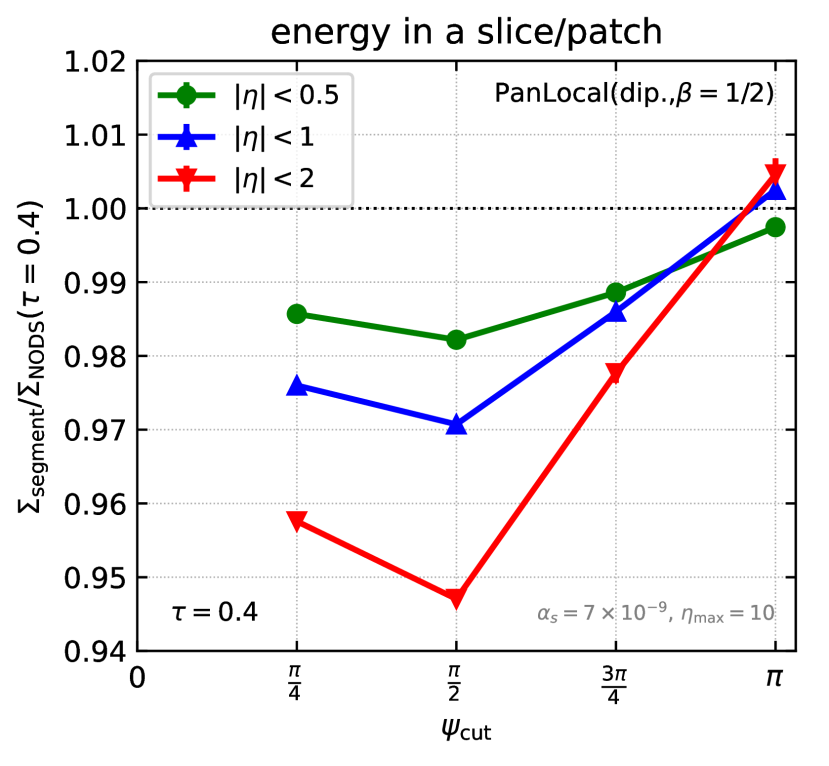
(a)

(b)

Figure 17: (a) Ratio between the segment and NODS methods for the energy deposited in a square patch of finite rapidity and azimuthal extent, as a function of $\tau$ defined in Eq. (57). The bands correspond to the statistical uncertainty. (b) Same shown as a function of the azimuthal extent of the patch for different rapidity widths and for $\tau=0.4$.

When comparing our subleading-colour results in section 7.3 for the energy in a rapidity slice to the full-colour ones obtained by Hatta and Ueda Hatta:2013iba , the apparent agreement between the segment and NODS methods might come as a surprise, given that the NODS method reproduces the full-colour double real energy-ordered soft matrix element, while the segment method does not. The difference between the methods is clearly visible in our matrix-element tests, see e.g. Fig. 4. For the energy in a rapidity slice, this means that the segment method should deviate from the full-$N_{\text{{c}}}$ result from ${\cal{O}}(\alpha_{s}^{2}L^{2})$ onwards, one order earlier than the NODS method for which deviations are expected from ${\cal{O}}(\alpha_{s}^{3}L^{3})$.

One possible explanation for the similarity between the segment and NODS methods for the rapidity slice observable is that the ${\cal{O}}(\alpha_{s}^{2}L^{2})$ deviation in the segment method largely disappears when integrating over the azimuthal angle of the two emissions. To test this hypothesis, we study the energy deposited in a rectangular patch of both finite rapidity and azimuthal extent, $|\eta|<\eta_{\text{cut}}=-\ln\tan\frac{\theta_{\text{cut}}}{2}$ and $|\psi|<\psi_{\text{cut}}$, thus breaking the azimuthal symmetry of the slice.

Fig. 17(a) shows the ratio between the segment and NODS methods for a patch of the same rapidity width as used in section 7.3 and different azimuthal extent. We see that while the difference between the two methods is smaller than 0.5% for the rapidity slice ($0.2\%$ at $\tau=0.4$), it can reach a few percent for a rectangular patch with finite $\psi$ extent. Among the patch extents we studied, $|\psi|<\frac{\pi}{2}$ showed the largest effect.

Finally, Fig. 17(b) shows the ratio between the segment and NODS schemes measured at $\tau=0.4$ for different rapidity and azimuthal extents. We notice that the deviation from 1 increases as the rapidity width of the patch increases, reaching $\sim 5\%$ for a patch with $|\eta|<2$ and $|\psi|<\frac{\pi}{2}$. The results here suggest that for future comparisons of non-global logarithms in methods implementing subleading-$N_{\text{{c}}}$ effects, it could be desirable to study not just slices but also patches.

References

- (1) G. Gustafson and U. Pettersson, Dipole Formulation of QCD Cascades, Nucl. Phys. B306 (1988) 746–758.
- (2) S. Platzer and M. Sjodahl, Subleading improved Parton Showers, JHEP 07 (2012) 042, [1201.0260].
- (3) Z. Nagy and D. E. Soper, Parton shower evolution with subleading color, JHEP 06 (2012) 044, [1202.4496].
- (4) Z. Nagy and D. E. Soper, Effects of subleading color in a parton shower, JHEP 07 (2015) 119, [1501.00778].
- (5) S. Plaetzer, M. Sjodahl and J. Thorén, Color matrix element corrections for parton showers, JHEP 11 (2018) 009, [1808.00332].
- (6) Z. Nagy and D. E. Soper, Parton showers with more exact color evolution, Phys. Rev. D 99 (2019) 054009, [1902.02105].
- (7) J. R. Forshaw, J. Holguin and S. Plätzer, Parton branching at amplitude level, JHEP 08 (2019) 145, [1905.08686].
- (8) M. De Angelis, J. R. Forshaw and S. Plätzer, Resummation and simulation of soft gluon effects beyond leading colour, 2007.09648.
- (9) S. Hoeche and D. Reichelt, Numerical resummation at full color in the strongly ordered soft gluon limit, 2001.11492.
- (10) J. Holguin, J. R. Forshaw and S. Plätzer, Comments on a new ‘full colour’ parton shower, 2003.06399.
- (11) M. Dasgupta, F. A. Dreyer, K. Hamilton, P. F. Monni and G. P. Salam, Logarithmic accuracy of parton showers: a fixed-order study, JHEP 09 (2018) 033, [1805.09327].
- (12) M. Dasgupta, F. A. Dreyer, K. Hamilton, P. F. Monni, G. P. Salam and G. Soyez, Parton showers beyond leading logarithmic accuracy, Phys. Rev. Lett. 125 (2020) 052002, [2002.11114].
- (13) B. Andersson, G. Gustafson, L. Lonnblad and U. Pettersson, Coherence Effects in Deep Inelastic Scattering, Z. Phys. C43 (1989) 625.
- (14) S. Catani, L. Trentadue, G. Turnock and B. R. Webber, Resummation of large logarithms in e+ e- event shape distributions, Nucl. Phys. B407 (1993) 3–42.
- (15) Z. Nagy and D. E. Soper, Summations of large logarithms by parton showers, 2011.04773.
- (16) Z. Nagy and D. E. Soper, Summations by parton showers of large logarithms in electron-positron annihilation, 2011.04777.
- (17) J. R. Forshaw, J. Holguin and S. Plätzer, Building a consistent parton shower, JHEP 09 (2020) 014, [2003.06400].
- (18) G. Marchesini and B. R. Webber, Monte Carlo Simulation of General Hard Processes with Coherent QCD Radiation, Nucl. Phys. B310 (1988) 461–526.
- (19) G. Corcella, I. G. Knowles, G. Marchesini, S. Moretti, K. Odagiri, P. Richardson et al., HERWIG 6: An Event generator for hadron emission reactions with interfering gluons (including supersymmetric processes), JHEP 01 (2001) 010, [hep-ph/0011363].
- (20) J. Bellm et al., Herwig 7.2 release note, Eur. Phys. J. C 80 (2020) 452, [1912.06509].
- (21) G. Bewick, S. Ferrario Ravasio, P. Richardson and M. H. Seymour, Logarithmic Accuracy of Angular-Ordered Parton Showers, 1904.11866.
- (22) M. Dasgupta and G. Salam, Resummation of nonglobal QCD observables, Phys. Lett. B 512 (2001) 323–330, [hep-ph/0104277].
- (23) A. Banfi, G. Corcella and M. Dasgupta, Angular ordering and parton showers for non-global QCD observables, JHEP 03 (2007) 050, [hep-ph/0612282].
- (24) G. Gustafson, Multiplicity distributions in QCD cascades, Nucl. Phys. B392 (1993) 251–280.
- (25) C. Friberg, G. Gustafson and J. Hakkinen, Color connections in annihilation, Nucl. Phys. B490 (1997) 289–305, [hep-ph/9604347].
- (26) B. R. Webber, “Jet rates from parton showers.” 2015 (unpublished, presented at “Taming the accuracy of event generators”, June 2020).
- (27) Z. Nagy and D. Soper, “Leading double logs for four jet production in annihilation.” 2015 (unpublished, presented at “Taming the accuracy of event generators”, June 2020).
- (28) Y. Hatta and T. Ueda, Resummation of non-global logarithms at finite , Nucl. Phys. B874 (2013) 808–820, [1304.6930].
- (29) F. A. Dreyer, G. P. Salam and G. Soyez, The Lund Jet Plane, JHEP 12 (2018) 064, [1807.04758].
- (30) J. Botts and G. F. Sterman, Hard Elastic Scattering in QCD: Leading Behavior, Nucl. Phys. B 325 (1989) 62–100.
- (31) J. R. Forshaw, A. Kyrieleis and M. H. Seymour, Super-leading logarithms in non-global observables in QCD, JHEP 08 (2006) 059, [hep-ph/0604094].
- (32) S. Catani, D. de Florian and G. Rodrigo, Space-like (versus time-like) collinear limits in QCD: Is factorization violated?, JHEP 07 (2012) 026, [1112.4405].
- (33) Z. Nagy and D. E. Soper, Exponentiating virtual imaginary contributions in a parton shower, Phys. Rev. D100 (2019) 074005, [1908.11420].
- (34) L. Lonnblad, ARIADNE version 4: A Program for simulation of QCD cascades implementing the color dipole model, Comput. Phys. Commun. 71 (1992) 15–31.
- (35) Z. Nagy and D. E. Soper, Parton showers with quantum interference: Leading color, with spin, JHEP 07 (2008) 025, [0805.0216].
- (36) T. Sjostrand and P. Z. Skands, Transverse-momentum-ordered showers and interleaved multiple interactions, Eur. Phys. J. C39 (2005) 129–154, [hep-ph/0408302].
- (37) T. Sjöstrand, S. Ask, J. R. Christiansen, R. Corke, N. Desai, P. Ilten et al., An Introduction to PYTHIA 8.2, Comput. Phys. Commun. 191 (2015) 159–177, [1410.3012].
- (38) G. Marchesini and B. R. Webber, Simulation of QCD Jets Including Soft Gluon Interference, Nucl. Phys. B238 (1984) 1–29.
- (39) Y. L. Dokshitzer, V. A. Khoze, A. H. Mueller and S. Troian, Basics of perturbative QCD. Editions frontières, 1991.
- (40) R. K. Ellis, W. J. Stirling and B. R. Webber, QCD and Collider Physics. Cambridge Monographs on Particle Physics, Nuclear Physics and Cosmology. Cambridge University Press, 1996. 10.1017/CBO9780511628788.
- (41) W. T. Giele, D. A. Kosower and P. Z. Skands, Higher-Order Corrections to Timelike Jets, Phys. Rev. D84 (2011) 054003, [1102.2126].
- (42) S. Hoeche and S. Prestel, The midpoint between dipole and parton showers, Eur. Phys. J. C75 (2015) 461, [1506.05057].
- (43) Y. L. Dokshitzer, G. D. Leder, S. Moretti and B. R. Webber, Better jet clustering algorithms, JHEP 08 (1997) 001, [hep-ph/9707323].
- (44) M. Wobisch and T. Wengler, Hadronization corrections to jet cross-sections in deep inelastic scattering, in Workshop on Monte Carlo Generators for HERA Physics (Plenary Starting Meeting), pp. 270–279, 4, 1998. hep-ph/9907280.
- (45) K. Chetyrkin, J. H. Kuhn and C. Sturm, QCD decoupling at four loops, Nucl. Phys. B 744 (2006) 121–135, [hep-ph/0512060].
- (46) P. Baikov, K. Chetyrkin and J. Kühn, Five-Loop Running of the QCD coupling constant, Phys. Rev. Lett. 118 (2017) 082002, [1606.08659].
- (47) T. Luthe, A. Maier, P. Marquard and Y. Schröder, Towards the five-loop Beta function for a general gauge group, JHEP 07 (2016) 127, [1606.08662].
- (48) F. Herzog, B. Ruijl, T. Ueda, J. Vermaseren and A. Vogt, The five-loop beta function of Yang-Mills theory with fermions, JHEP 02 (2017) 090, [1701.01404].
- (49) L. Lönnblad, Fooling Around with the Sudakov Veto Algorithm, Eur. Phys. J. C 73 (2013) 2350, [1211.7204].
- (50) Y. Hida, X. S. Li and D. H. Bailey, Quad-double arithmetic: Algorithms, implementation, and application, in 15th IEEE Symposium on Computer Arithmetic, pp. 155–162, 2000.
- (51) L. Fousse, G. Hanrot, V. Lefèvre, P. Pélissier and P. Zimmermann, MPFR: a multiple-precision binary floating-point library with correct rounding, ACM Transactions on Mathematical Software (TOMS) 33 (2007) 13–es.
- (52) S. Catani, Y. L. Dokshitzer, F. Fiorani and B. R. Webber, Average number of jets in e+ e- annihilation, Nucl. Phys. B377 (1992) 445–460.
- (53) S. Catani, Y. L. Dokshitzer, M. Olsson, G. Turnock and B. R. Webber, New clustering algorithm for multi - jet cross-sections in annihilation, Phys. Lett. B269 (1991) 432–438.
- (54) S. Catani, G. Turnock and B. R. Webber, Jet broadening measures in annihilation, Phys. Lett. B295 (1992) 269–276.
- (55) E. Farhi, A QCD Test for Jets, Phys. Rev. Lett. 39 (1977) 1587–1588.
- (56) A. Banfi, G. P. Salam and G. Zanderighi, Principles of general final-state resummation and automated implementation, JHEP 03 (2005) 073, [hep-ph/0407286].
- (57) A. Banfi, G. Marchesini, Y. L. Dokshitzer and G. Zanderighi, QCD analysis of near-to-planar three jet events, JHEP 07 (2000) 002, [hep-ph/0004027].
- (58) A. Banfi, Y. L. Dokshitzer, G. Marchesini and G. Zanderighi, QCD analysis of D parameter in near to planar three jet events, JHEP 05 (2001) 040, [hep-ph/0104162].
- (59) M. Dasgupta and G. P. Salam, Accounting for coherence in interjet E(t) flow: A Case study, JHEP 03 (2002) 017, [hep-ph/0203009].
- (60) A. Banfi, G. Marchesini and G. Smye, Away from jet energy flow, JHEP 08 (2002) 006, [hep-ph/0206076].
- (61) H. Weigert, Nonglobal jet evolution at finite N(c), Nucl. Phys. B 685 (2004) 321–350, [hep-ph/0312050].
- (62) Y. Hagiwara, Y. Hatta and T. Ueda, Hemisphere jet mass distribution at finite , Phys. Lett. B 756 (2016) 254–258, [1507.07641].
- (63) Y. Hatta and T. Ueda, Non-global logarithms in hadron collisions at , 2011.04154.