Formation of turbulence via an interaction potential

Abstract.

In a recent work, we proposed a hypothesis that the turbulence in gases could be produced by particles interacting via a potential – for example, the interatomic potential at short ranges, and the electrostatic potential at long ranges. Here, we examine the proposed mechanics of turbulence formation in a simple model of two particles, which interact solely via a potential. Following the kinetic theory approach, we derive a hierarchy of the velocity moment transport equations, and then truncate it via a novel closure based on the high Reynolds number condition. While standard closures of the velocity moment hierarchy of the Boltzmann equation lead to the compressible Euler and Navier–Stokes systems of equations, our closure leads to a transport equation for the velocity alone, which is driven by the potential forcing. Starting from a large scale laminar shear flow, we numerically simulate the solutions of our velocity transport equation for the electrostatic, gravity, Thomas–Fermi and Lennard-Jones potentials, as well as the Vlasov-type large scale mean field potential. In all studied scenarios, the time-averaged Fourier spectra of the kinetic energy clearly exhibit Kolmogorov’s “five-thirds” power decay rate.

1. Introduction

In our recent work [3], we proposed a hypothesis that the turbulence in gases could be produced by their particles interacting via a potential. The reason why we proposed such an unusual hypothesis is the following. We investigated the dynamical system consisting of many particles interacting via a potential, without reducing it to a single-particle equation as typically done in the conventional kinetic theory. We found that, due to the presence of the potential, a strong large scale flow creates the forcing in the three-dimensional bundles of the full coordinate space, with each bundle belonging to a pair of particles. At the same time, in the Boltzmann equation [7, 12], the potential interactions are replaced with the collision integral, which results in the absence of the potential forcing terms in the standard equations of fluid mechanics, such as the Euler [5] or Navier–Stokes [14] equations.

However, we noted that the direct observations and measurements of a turbulent fluid can register some bulk properties of the induced flow in these particle-pair bundles, such as the power scaling of the Fourier transform of the kinetic energy of the flow. In our work [3], we made crude estimates of the power scaling of the kinetic energy in the inertial range, induced by a strong large scale flow via the interaction potential. Remarkably, we found our crude estimates to be consistent with direct measurements and observations [10, 22].

Our results [3] further motivated us to look for a more detailed explanation of how the turbulence could be induced by a strong large scale flow via an interaction potential. In the current work, we develop and implement a simple fluid mechanical model of behavior of a pair of particles, which interact solely via a potential. While we recognize that, in the real world natural phenomena, the dynamics are much more complex with multiple types of interactions, the primary goal of the current work is to investigate whether an interaction potential alone by itself can produce flow structures with power decay of the Fourier transforms of dynamical variables. If needed, an extension onto many particles can be made in a standard fashion via the Bogoliubov–Born–Green–Kirkwood–Yvon [6, 8, 16] hierarchy approach.

The paper is organized as follows. In Section 2, we start with the equations of motion for a system of two particles, which interact via a potential. For this system, we compute the Liouville equation, the thermodynamic equilibrium state of the system, and show that a generic solution preserves the “distance” to the equilibrium state in the sense of any of the Rényi metrics [26], which is similar to the effect of Boltzmann’s $H$-theorem [7] for hard-sphere gases. We change the variables from the coordinate and velocity of each individual particle to those of the center of mass of the system and the difference between the particles. We then exclude the motion of the center of mass from the dynamics, which leads to the Liouville equation for the turbulent variables (that is, those which represent the differences in the coordinates and velocities between the particles). Alternatively, we integrate out the second particle, and arrive at the Vlasov equation [31] for a single particle, which has the same form as the Liouville equation for the turbulent variables.

In Section 3, we formulate a hierarchy of the transport equations for the velocity moments of the turbulent Liouville or Vlasov equations. However, due to the fact that the potential forcing replaces the usual Boltzmann collision integral, a different closure must be used to truncate the moment hierarchy. Here, we introduce a novel closure based on the high Reynolds number condition, which leads to a single equation for the turbulent velocity, driven by the potential forcing. This corresponds well with the fact that the observed turbulence appears to have largely universal behavior across a variety of different media. However, due to the simplicity of our model, the turbulent velocity equation lacks dissipation, and thus its solutions are meaningful on a limited time scale.

In Section 4 we show the results of numerical simulations of the turbulent velocity equation, which all start with a large scale laminar shear flow as the initial condition, and are forced by different types of the interaction potential. We examine the scenarios for the following interaction potentials: electrostatic, gravitational, Thomas–Fermi [30, 13], Lennard-Jones [21], as well as the Vlasov-type large scale mean field potential. In each scenario, we discover the regime of secular growth which precludes the exponential blow-up (the latter due to the lack of dissipation). For all scenarios, in this secular growth regime, the time-averaged Fourier transforms of the kinetic energy of the flow decay as the negative five-thirds power of the wavenumber, which matches the Kolmogorov turbulence spectrum [17, 18, 19, 23, 24, 25]. The results of this work are summarized in Section 5. The generalizations onto multiparticle systems are sketched in Appendices A, B and C.

2. Particle dynamics

In our attempt to uncover the origins of the turbulent kinetic energy spectra, we follow the general approach of kinetic theory, starting with the elementary evolution mechanics of particles which interact solely via a potential. First, we consider a simple model of only two interacting particles, thereby avoiding the multiparticle closure problem, and derive the Liouville equation for this pair of particles. Second, we derive the Vlasov equation for one of the particles in the pair, by using a simple closure for another particle. The generalizations of what is presented here onto a multiparticle set-up are given in Appendices A, B and C.

2.1. Two particle dynamics

Let the two identical particles, with coordinates $\boldsymbol{x}_{1}$ and $\boldsymbol{x}_{2}$, and velocities $\boldsymbol{v}_{1}$ and $\boldsymbol{v}_{2}$, respectively, interact via a potential $\phi(r)$. The equations of motion for these two particles are given via

(2.1a) $$\frac{\mathrm{d}\boldsymbol{x}_{1}}{\mathrm{d}t}=\boldsymbol{v}_{1},\qquad\frac{\mathrm{d}\boldsymbol{v}_{1}}{\mathrm{d}t}=-\frac{\partial}{\partial\boldsymbol{x}_{1}}\phi(\|\boldsymbol{x}_{2}-\boldsymbol{x}_{1}\|),$$

(2.1b) $$\frac{\mathrm{d}\boldsymbol{x}_{2}}{\mathrm{d}t}=\boldsymbol{v}_{2},\qquad\frac{\mathrm{d}\boldsymbol{v}_{2}}{\mathrm{d}t}=-\frac{\partial}{\partial\boldsymbol{x}_{2}}\phi(\|\boldsymbol{x}_{2}-\boldsymbol{x}_{1}\|).$$

Here we make two assumptions, which simplify further manipulations. First, we assume that the coordinate domain is of finite volume, but has no discernible boundaries (e.g. a periodic cube). Second, we assume that the potential $\phi(r)$ does not have a singularity at zero, although it may still peak strongly as $r\to 0$ to model either repulsion or attraction, whichever is needed in the context of the problem.

It is easy to see that the dynamics in (2.1) preserve the momentum and energy of the system of two particles:

(2.2) $$\boldsymbol{v}_{1}+\boldsymbol{v}_{2}=\text{const},\qquad\|\boldsymbol{v}_{1}\|^{2}+\|\boldsymbol{v}_{2}\|^{2}+2\phi(\|\boldsymbol{x}_{2}-\boldsymbol{x}_{1}\|)=\text{const}.$$

For a given value of the momentum, it is always possible to choose the inertial reference frame in which the momentum becomes zero (the so-called Galilean shift). Thus, without much loss of generality, we will further assume that the total momentum of the system of the two particles is zero.

2.2. The Liouville equation

Let $f(t,\boldsymbol{x}_{1},\boldsymbol{v}_{1},\boldsymbol{x}_{2},\boldsymbol{v}_{2})$ denote the distribution density of states of (2.1). Then, the transport equation for $f$, known as the Liouville equation, is given via

(2.3) $$\frac{\partial f}{\partial t}+\boldsymbol{v}_{1}\cdot\frac{\partial f}{\partial\boldsymbol{x}_{1}}+\boldsymbol{v}_{2}\cdot\frac{\partial f}{\partial\boldsymbol{x}_{2}}=\frac{\partial}{\partial\boldsymbol{x}_{1}}\phi(\|\boldsymbol{x}_{2}-\boldsymbol{x}_{1}\|)\cdot\frac{\partial f}{\partial\boldsymbol{v}_{1}}+\frac{\partial}{\partial\boldsymbol{x}_{2}}\phi(\|\boldsymbol{x}_{2}-\boldsymbol{x}_{1}\|)\cdot\frac{\partial f}{\partial\boldsymbol{v}_{2}}.$$

One can verify that any suitable function of the form

(2.4) $$f_{0}(\boldsymbol{x}_{1},\boldsymbol{v}_{1},\boldsymbol{x}_{2},\boldsymbol{v}_{2})=g\big{(}\|\boldsymbol{v}_{1}\|^{2}+\|\boldsymbol{v}_{2}\|^{2}+2\phi(\|\boldsymbol{x}_{2}-\boldsymbol{x}_{1}\|)\big{)}$$

is a steady state. Among all such states, the canonical Gibbs state is given via

(2.5) $$f_{G}(\boldsymbol{x}_{1},\boldsymbol{v}_{1},\boldsymbol{x}_{2},\boldsymbol{v}_{2})=\frac{1}{(2\pi\theta_{0})^{3}Z}\exp\left(-\frac{\|\boldsymbol{v}_{1}\|^{2}+\|\boldsymbol{v}_{2}\|^{2}+2\phi(\|\boldsymbol{x}_{2}-\boldsymbol{x}_{1}\|)}{2\theta_{0}}\right),$$

where $\theta_{0}$ is the kinetic temperature of the system, and $Z$ is the spatial normalization constant:

(2.6) $$Z=\int e^{-\phi(\|\boldsymbol{x}_{2}-\boldsymbol{x}_{1}\|)/\theta_{0}}\>\!\mathrm{d}\boldsymbol{x}_{1}\>\!\mathrm{d}\boldsymbol{x}_{2}.$$

2.3. Preservation of the Rényi divergence

It is important to note that the Liouville equation preserves the family of Rényi divergences [26] between a solution $f$ and a steady state $f_{0}$. Indeed, let $\psi_{1}:\mathbb{R}\to\mathbb{R}$, $\psi_{2}:\mathbb{R}\to\mathbb{R}$ be two differentiable functions. In the absence of boundary effects, any quantity of the form

(2.7) $$\int\psi_{1}(f)\psi_{2}(f_{0})\>\!\mathrm{d}\boldsymbol{x}_{1}\>\!\mathrm{d}\boldsymbol{v}_{1}\>\!\mathrm{d}\boldsymbol{x}_{2}\>\!\mathrm{d}\boldsymbol{v}_{2}$$

is preserved in time. Indeed, the time derivative yields the following chain of identities (the measure notations are omitted to save space):

(2.8) $$\frac{\partial}{\partial t}\int\psi_{1}(f)\psi_{2}(f_{0})=\int\psi_{2}(f_{0})\frac{\partial\psi_{1}(f)}{\partial t}=\int\psi_{2}(f_{0})\bigg{(}\frac{\partial\phi}{\partial(\boldsymbol{x}_{1},\boldsymbol{x}_{2})}\cdot\frac{\partial\psi_{1}(f)}{\partial(\boldsymbol{v}_{1},\boldsymbol{v}_{2})}-\\ -(\boldsymbol{v}_{1},\boldsymbol{v}_{2})\cdot\frac{\partial\psi_{1}(f)}{\partial(\boldsymbol{x}_{1},\boldsymbol{x}_{2})}\bigg{)}=\int\psi_{1}(f)\bigg{(}(\boldsymbol{v}_{1},\boldsymbol{v}_{2})\cdot\frac{\partial\psi_{2}(f_{0})}{\partial(\boldsymbol{x}_{1},\boldsymbol{x}_{2})}-\frac{\partial\phi}{\partial(\boldsymbol{x}_{1},\boldsymbol{x}_{2})}\cdot\frac{\partial\psi_{2}(f_{0})}{\partial(\boldsymbol{v}_{1},\boldsymbol{v}_{2})}\bigg{)}=0.$$

In particular, taking $\psi_{1}(x)=x^{\alpha}$, $\psi_{2}(x)=x^{1-\alpha}$, for some $\alpha>0$, demonstrates that the family of general Rényi divergences is preserved in time:

(2.9) $$D_{\alpha}(f,f_{0})=\frac{1}{\alpha-1}\ln\int f^{\alpha}f_{0}^{1-\alpha}\>\!\mathrm{d}\boldsymbol{x}_{1}\>\!\mathrm{d}\boldsymbol{v}_{1}\>\!\mathrm{d}\boldsymbol{x}_{2}\>\!\mathrm{d}\boldsymbol{v}_{2}=\text{const}.$$

The Kullback–Leibler divergence [20] is a special case of the Rényi divergence with $\alpha=1$.

The above result shows that, in the absence of external or boundary effects, and irreversible interactions, the dynamical system in (2.1) retains is initial “distance” to any steady state $f_{0}$ in the sense of the Rényi metric (2.9). In particular, if it starts near the Gibbs equilibrium (2.5), then it will remain so throughout its time evolution.

2.4. Mean and turbulent variables

Let us make the following change of variables:

(2.10) $$\boldsymbol{x}=\boldsymbol{x}_{2}-\boldsymbol{x}_{1},\qquad\boldsymbol{v}=\boldsymbol{v}_{2}-\boldsymbol{v}_{1},\qquad\boldsymbol{y}=\frac{\boldsymbol{x}_{1}+\boldsymbol{x}_{2}}{2},\qquad\boldsymbol{w}=\frac{\boldsymbol{v}_{1}+\boldsymbol{v}_{2}}{2}.$$

Here, $\boldsymbol{y}$ and $\boldsymbol{w}$ describe the motion of the center of mass of the system (and thus can be viewed as the “mean” variables), while $\boldsymbol{x}$ and $\boldsymbol{v}$ describe the relative motions of one particle with respect to another, and thus are regarded as the “turbulent” variables. In the new variables, the partial derivatives become

(2.11a) $$\frac{\partial}{\partial\boldsymbol{x}_{1}}=-\frac{\partial}{\partial\boldsymbol{x}}+\frac{1}{2}\frac{\partial}{\partial\boldsymbol{y}},\qquad\frac{\partial}{\partial\boldsymbol{v}_{1}}=-\frac{\partial}{\partial\boldsymbol{v}}+\frac{1}{2}\frac{\partial}{\partial\boldsymbol{w}},$$

(2.11b) $$\frac{\partial}{\partial\boldsymbol{x}_{2}}=\frac{\partial}{\partial\boldsymbol{x}}+\frac{1}{2}\frac{\partial}{\partial\boldsymbol{y}},\qquad\frac{\partial}{\partial\boldsymbol{v}_{2}}=\frac{\partial}{\partial\boldsymbol{v}}+\frac{1}{2}\frac{\partial}{\partial\boldsymbol{w}}.$$

Substituting the expressions above into the Liouville equation for $f$, we arrive at

(2.12) $$\frac{\partial f}{\partial t}+\boldsymbol{v}\cdot\frac{\partial f}{\partial\boldsymbol{x}}+\boldsymbol{w}\cdot\frac{\partial f}{\partial\boldsymbol{y}}=2\frac{\partial\phi(\|\boldsymbol{x}\|)}{\partial\boldsymbol{x}}\cdot\frac{\partial f}{\partial\boldsymbol{v}}.$$

Observe that the total momentum variable $\boldsymbol{w}$ is merely a constant parameter, because there are no derivatives with respect to it. Since we consider the dynamics of (2.1) with zero total momentum, we have to set $\boldsymbol{w}=\boldsymbol{0}$ above. This leads to the following Liouville equation for $f$:

(2.13) $$\frac{\partial f}{\partial t}+\boldsymbol{v}\cdot\frac{\partial f}{\partial\boldsymbol{x}}=2\frac{\partial\phi(\|\boldsymbol{x}\|)}{\partial\boldsymbol{x}}\cdot\frac{\partial f}{\partial\boldsymbol{v}}.$$

Observe that dependence of $f$ on $\boldsymbol{y}$ and $\boldsymbol{w}$ no longer matters, and further we assume that $f$ is only a function of $t$, $\boldsymbol{x}$ and $\boldsymbol{v}$. The general steady state of (2.13) is given via

(2.14) $$f_{0}(\boldsymbol{x},\boldsymbol{v})=g\big{(}\|\boldsymbol{v}\|^{2}+4\phi(\|\boldsymbol{x}\|)\big{)},$$

with the corresponding Gibbs state being

(2.15) $$f_{G}(\boldsymbol{x},\boldsymbol{v})=\frac{1}{(4\pi\theta_{0})^{3}Z}\exp\left(-\frac{\|\boldsymbol{v}\|^{2}+4\phi(\|\boldsymbol{x}\|)}{4\theta_{0}}\right),\qquad Z=\int e^{-\phi(\|\boldsymbol{x}\|)/\theta_{0}}\>\!\mathrm{d}\boldsymbol{x}.$$

The reason why $\theta_{0}$ is multiplied by a factor of 4 in the denominator (instead of the usual 2) is because

(2.16) $$\|\boldsymbol{v}\|^{2}=\|\boldsymbol{v}_{2}-\boldsymbol{v}_{1}\|^{2}=\|\boldsymbol{v}_{2}-\boldsymbol{v}_{1}\|^{2}+\|\boldsymbol{v}_{1}+\boldsymbol{v}_{2}\|^{2}=2(\|\boldsymbol{v}_{1}\|^{2}+\|\boldsymbol{v}_{2}\|^{2}),$$

where we use the fact that the total momentum of the system is zero. So, if $\theta_{0}$ is the energy per degree of freedom per particle, then the corresponding “temperature of the difference” between the two particles must be twice that value.

Clearly, the Liouville equation (2.13) also preserves the family of Rényi metrics in (2.9). This justifies the standard fluid-mechanical treatment of the dynamics via the velocity-moment hierarchy with a subsequent closure, which we apply further below.

2.5. Single particle dynamics (Vlasov equation)

The two-particle Liouville equation in (2.3) can be reduced to the single-particle Vlasov equation [31] with the help of a closure. Let us denote the first particle marginal density via

(2.17) $$f_{1}(\boldsymbol{x}_{1},\boldsymbol{v}_{1})=\int f(\boldsymbol{x}_{1},\boldsymbol{v}_{1},\boldsymbol{x}_{2},\boldsymbol{v}_{2})\>\!\mathrm{d}\boldsymbol{x}_{2}\>\!\mathrm{d}\boldsymbol{v}_{2}.$$

The transport equation for $f_{1}$ can be obtained by integrating the two-particle Liouville equation in (2.3) in $\>\!\mathrm{d}\boldsymbol{x}_{2}\>\!\mathrm{d}\boldsymbol{v}_{2}$:

(2.18) $$\frac{\partial f_{1}}{\partial t}+\boldsymbol{v}_{1}\cdot\frac{\partial f_{1}}{\partial\boldsymbol{x}_{1}}=\int\frac{\partial}{\partial\boldsymbol{x}_{1}}\phi(\|\boldsymbol{x}_{2}-\boldsymbol{x}_{1}\|)\cdot\frac{\partial f}{\partial\boldsymbol{v}_{1}}\>\!\mathrm{d}\boldsymbol{x}_{2}\>\!\mathrm{d}\boldsymbol{v}_{2}.$$

Observe that the right-hand side above still contains $f$, and we need a suitable closure to approximate it in terms of $f_{1}$. Here, we can use the same principle as we did in our earlier work [2]. Observe that the Gibbs state (2.5) can be written in the form

(2.19) $$f_{G}(\boldsymbol{x}_{1},\boldsymbol{v}_{1},\boldsymbol{x}_{2},\boldsymbol{v}_{2})=\frac{V^{2}}{Z}e^{-\phi(\|\boldsymbol{x}_{2}-\boldsymbol{x}_{1}\|)/\theta_{0}}f_{1,G}(\boldsymbol{v}_{1})f_{2,G}(\boldsymbol{v}_{2}),$$

where $f_{1,G}$ and $f_{2,G}$ are the single-particle marginal densities,

(2.20) $$f_{1,G}(\boldsymbol{v})=f_{2,G}(\boldsymbol{v})=\frac{1}{(2\pi\theta_{0})^{3/2}V}e^{-\|\boldsymbol{v}\|^{2}/2\theta_{0}},$$

and $V$ is the volume of the coordinate domain. If the state $f$ is close to the Gibbs equilibrium (2.5), we can assume that $f$ has the same marginal structure as (2.5) above:

(2.21) $$f(\boldsymbol{x}_{1},\boldsymbol{v}_{1},\boldsymbol{x}_{2},\boldsymbol{v}_{2})=\frac{V^{2}}{Z}e^{-\phi(\|\boldsymbol{x}_{2}-\boldsymbol{x}_{1}\|)/\theta_{0}}f_{1}(\boldsymbol{x}_{1},\boldsymbol{v}_{1})f_{2}(\boldsymbol{x}_{2},\boldsymbol{v}_{2}),$$

where $f_{2}$ is the marginal density of the second particle. Substituting the closure for $f$ in (2.21) into (2.18) yields the Vlasov equation for the marginal density of the first particle,

(2.22) $$\frac{\partial f_{1}}{\partial t}+\boldsymbol{v}\cdot\frac{\partial f_{1}}{\partial\boldsymbol{x}_{1}}=\frac{\partial\bar{\phi}(\boldsymbol{x}_{1})}{\partial\boldsymbol{x}_{1}}\cdot\frac{\partial f_{1}}{\partial\boldsymbol{v}_{1}},$$

with $\bar{\phi}$ being the following mean field potential:

(2.23) $$\bar{\phi}(\boldsymbol{x})=-\frac{V^{2}}{Z}\theta_{0}\int e^{-\phi(\|\boldsymbol{x}-\boldsymbol{y}\|)/\theta_{0}}\rho_{2}(\boldsymbol{y})\>\!\mathrm{d}\boldsymbol{y},\qquad\rho_{2}(\boldsymbol{y})=\int f_{2}(\boldsymbol{y},\boldsymbol{w})\>\!\mathrm{d}\boldsymbol{w}.$$

While here the derivation of the Vlasov equation is presented for the two-particle dynamics, in Appendix B we sketch the general procedure for a multiparticle system.

The chief difference between $\phi$ and $\bar{\phi}$ is that, in the convolution (2.23) for the latter, the mass density $\rho_{2}$ acts as a low-pass filter. Thus, even if $\phi$ has typical properties of an interaction potential (that is, peaked at zero, and a generally rich Fourier spectrum), the mean field potential $\bar{\phi}$ is a large scale potential, that is, it is confined to only a few large scale Fourier modes.

At the same time, the form of the Vlasov equation (2.22) is almost identical to that of the Liouville equation (2.13), with the only difference that the interaction potential $2\phi$ in the latter is replaced with $\bar{\phi}$ in the former. While we note that, generally, $\bar{\phi}$ is time-dependent (since it includes $\rho_{2}$), however, here it shall be assumed that, on the relevant time scales, $\bar{\phi}$ can be regarded as constant in time, and thus (2.13) and (2.22) can be treated in the same manner. So, while in what follows we refer chiefly to the Liouville equation in (2.13), it also applies to the Vlasov equation in (2.22).

3. The equation for the turbulent velocity

In the conventional approach to fluid mechanics, the Boltzmann equation is converted into a hierarchy of the transport equations for the velocity moments, which is subsequently truncated at a suitable point. Depending on where and how the moment hierarchy is truncated, one obtains the Euler equations [5], the Navier–Stokes equations [14], Grad’s 13-moment system [15], the regularization of Grad’s 13-moment system [29], etc. The main tool in justifying such a truncation of the moment hierarchy is Boltzmann’s $H$-theorem [7, 11, 12]. Namely, in the presence of the entropy growth, one argues that the distribution of the molecular velocities in the Boltzmann equation must approach the Maxwell–Boltzmann thermodynamic equilibrium state, and, therefore, only a relatively few low-order velocity moments are sufficient to accurately describe the overall shape of the solution.

In the present context, the role of the $H$-theorem is played by the conservation of the Rényi metrics in (2.9). Even though the solution of (2.13) does not approach the steady state (2.14) or (2.15), it also does not escape it, maintaining, instead, a constant “distance” to the latter in the sense of a Rényi metric. Clearly, if the initial condition of (2.13) is close, in the sense of (2.9), to (2.14) or (2.15), then the corresponding solution will also remain a nearby state. Thus, in what follows, we apply the velocity moment procedure to (2.13) in a similar way it is done conventionally.

We define the velocity average $\langle a\rangle$ of a function $a(\boldsymbol{v})$ via

(3.1) $$\langle a\rangle(t,\boldsymbol{x})=\int a(\boldsymbol{v})f(t,\boldsymbol{x},\boldsymbol{v})\>\!\mathrm{d}\boldsymbol{v}.$$

As usual, we denote the zero- and first-order velocity moments via the density $\rho$ and average velocity $\boldsymbol{u}$, respectively:

(3.2) $$\rho=\langle 1\rangle,\qquad\rho\boldsymbol{u}=\langle\boldsymbol{v}\rangle.$$

Then, for the moments of $f$ in (2.13) (or for those of $f_{1}$ in (2.22)), we integrate the potential forcing terms with $\boldsymbol{v}$-derivatives by parts, and obtain

(3.3a) $$\frac{\partial\rho}{\partial t}+\nabla\cdot(\rho\boldsymbol{u})=0,\qquad\frac{\partial(\rho\boldsymbol{u})}{\partial t}+\nabla\cdot\big{\langle}\boldsymbol{v}^{2}\big{\rangle}=-2\rho\nabla\phi,$$

(3.3b) $$\frac{\partial\langle\boldsymbol{v}^{2}\rangle}{\partial t}+\nabla\cdot\langle\boldsymbol{v}^{3}\rangle=-2\rho\big{(}\boldsymbol{u}\nabla\phi^{T}+\nabla\phi\boldsymbol{u}^{T}\big{)},$$

where $\boldsymbol{v}^{2}=\boldsymbol{v}\boldsymbol{v}^{T}$ is the outer product of $\boldsymbol{v}$ with itself, and the symmetric 3-rank tensor $\boldsymbol{v}^{3}$ is the outer product of $\boldsymbol{v}$ with itself, computed twice.

Next, let us decompose the quadratic moment $\langle\boldsymbol{v}^{2}\rangle$ as

(3.4) $$\langle\boldsymbol{v}^{2}\rangle=\rho\boldsymbol{u}^{2}+\langle(\boldsymbol{v}-\boldsymbol{u})^{2}\rangle,\quad\text{with}\quad\langle(\boldsymbol{v}-\boldsymbol{u})^{2}\rangle=\rho(\theta\mathsfbi I+\mathsfbi S).$$

Above, $\theta$ is the kinetic temperature of $\boldsymbol{v}$, given via the trace of the centered quadratic moment,

(3.5) $$\rho\theta=\frac{1}{3}\mathrm{tr}\langle(\boldsymbol{v}-\boldsymbol{u})^{2}\rangle=\frac{1}{3}\langle\|\boldsymbol{v}-\boldsymbol{u}\|^{2}\rangle,$$

while the matrix $\mathsfbi S$ is called the shear stress, and quantifies the deviation of the centered quadratic moment from its own trace. By construction, the trace of $\mathsfbi S$ is zero. The product $\rho\theta$ is known as the pressure.

Similar manipulations can be made for the cubic moment. Here, we decompose

(3.6) $$\langle\boldsymbol{v}^{3}\rangle=\rho\Big{(}\boldsymbol{u}^{3}+(\theta\mathsfbi I+\mathsfbi S)\otimes\boldsymbol{u}+\big{(}(\theta\mathsfbi I+\mathsfbi S)\otimes\boldsymbol{u}\big{)}^{T}+\big{(}(\theta\mathsfbi I+\mathsfbi S)\otimes\boldsymbol{u}\big{)}^{TT}\Big{)}+\langle(\boldsymbol{v}-\boldsymbol{u})^{3}\rangle,$$

where “$T$” and “$TT$” denote the two cyclic permutations of a 3-rank tensor, and “$\otimes$” denotes an outer product. In turn, the skewness (that is, the centered cubic moment) $\langle(\boldsymbol{v}-\boldsymbol{u})^{3}\rangle$ can be expressed via

(3.7) $$\langle(\boldsymbol{v}-\boldsymbol{u})^{3}\rangle=\frac{2}{5}\rho\big{(}\boldsymbol{q}\otimes\mathsfbi I+(\boldsymbol{q}\otimes\mathsfbi I)^{T}+(\boldsymbol{q}\otimes\mathsfbi I)^{TT}\big{)}+\rho\mathsfbi Q.$$

Above, $\boldsymbol{q}$ is the conductive heat flux, given via

(3.8) $$\rho\boldsymbol{q}=\frac{1}{2}\langle\|\boldsymbol{v}-\boldsymbol{u}\|^{2}(\boldsymbol{v}-\boldsymbol{u})\rangle,$$

while $\mathsfbi Q$ is the deviator between the heat flux and the skewness tensor. Observe that $\mathsfbi Q$ is a symmetric 3-rank tensor whose contraction along any pair of indices is zero. This is due to the fact that the heat flux $\boldsymbol{q}$ is itself a multiple of the contracted skewness moment:

(3.9) $$(\rho\boldsymbol{q})_{i}=\frac{1}{2}\sum_{j=1}^{3}\langle(\boldsymbol{v}-\boldsymbol{u})^{3}\rangle_{jji}.$$

The deviator $\mathsfbi Q$ is related to the centered cubic moment in the same way as the shear stress $\mathsfbi S$ is related to the centered quadratic moment – namely, $\mathsfbi Q$ quantifies the deviation of the skewness $\langle(\boldsymbol{v}-\boldsymbol{u})^{3}\rangle$ from its own trace along any pair of its indices.

3.1. Nondimensionalization and scalings

Following the standard approach in fluid mechanics, here we need to choose suitable closures for $\mathsfbi S$ and $\boldsymbol{q}$. If the irreversible collisions are present in the form of a Boltzmann collision integral, one can assume that $\mathsfbi S$ and $\boldsymbol{q}$ are the steady states of their respective transport equations [14, 15]. Such a formalism yields the Newton law of viscosity, and the Fourier law of heat conduction. In our situation, however, there are no collision integrals, and an analogous closure cannot be used. Instead, here we close the velocity moment hierarchy in a novel way, making use of the well-established criterion which holds systematically for observed turbulent flows – namely, the high Reynolds number condition.

Let $L$ and $U$ denote, respectively, the characteristic length scale of the flow, and its reference speed, such that the ratio $U/L$ specifies the characteristic time scale. First, we rescale the time and space differentiation operators, as well as the velocity, via

(3.10) $$\nabla\to\frac{1}{L}\nabla,\qquad\frac{\partial}{\partial t}\to\frac{U}{L}\frac{\partial}{\partial t},\qquad\boldsymbol{u}\to U\boldsymbol{u}.$$

It is easy to see that the mass transport equation in (3.3a) is invariant with respect to this scaling. Also, observe that it is pointless to rescale the density $\rho$ (as the scaling constant would simply factor out of all transport equations), and thus we leave it as is.

In the momentum equation, we need to choose the scalings for $\phi$, $\theta$ and $\mathsfbi S$. For the potential $\phi$ and temperature $\theta$, we choose the reference temperature constant $T$. The treatment of the viscous shear stress $\mathsfbi S$ must be different, since it quantifies an entirely different physical property – namely, while the temperature is related to the force which a fluid exerts onto a plate in the orthogonal direction (the pressure), the shear stress quantifies the tangential force of resistance to a shear (similar to friction). Therefore, to rescale the stress $\mathsfbi S$, we introduce a reference constant $\mathcal{V}$ which has the units of the kinematic viscosity (that is, squared length over time), and choose the following scaling:

(3.11) $$\phi\to T\phi,\qquad\theta\to T\theta,\qquad\mathsfbi S\to\frac{\mathcal{V}U}{L}\mathsfbi S.$$

In the rescaled variables, the momentum equation in (3.3a) becomes

(3.12) $$\frac{\partial(\rho\boldsymbol{u})}{\partial t}+\nabla\cdot\bigg{(}\rho\boldsymbol{u}^{2}+\frac{1}{\textit{Ma}^{2}}\rho\theta\mathsfbi I+\frac{1}{\textit{Re}}\rho\mathsfbi S\bigg{)}=-\frac{2}{\textit{Ma}^{2}}\rho\nabla\phi,$$

where Ma and Re are the Mach and Reynolds numbers, respectively:

(3.13) $$\textit{Ma}=\frac{U}{\sqrt{T}},\qquad\textit{Re}=\frac{UL}{\mathcal{V}}.$$

Here note that our definition of the Mach number differs from the traditional one by the square root of the adiabatic constant, for convenience. For the transport of higher-order moments, we need to choose the scalings for $\boldsymbol{q}$ and $\mathsfbi Q$. In the absence of any particular information about the difference in magnitudes between $\boldsymbol{q}$ and $\mathsfbi Q$, we choose the rescaling for each quantity in the same manner as above for $\theta$, with the additional multiplication by the reference speed $U$ so that the physical units remain consistent:

(3.14) $$\boldsymbol{q}\to TU\boldsymbol{q},\qquad\mathsfbi Q\to TU\mathsfbi Q.$$

Then, the transport equations for the pressure $\rho\theta$ and the shear stress $\mathsfbi S$ become

(3.15a) $$\frac{\partial(\rho\theta)}{\partial t}+\nabla\cdot(\rho\theta\boldsymbol{u})+\frac{2}{3}\bigg{[}\rho\bigg{(}\theta\mathsfbi I+\frac{\textit{Ma}^{2}}{\textit{Re}}\mathsfbi S\bigg{)}:\nabla\boldsymbol{u}+\nabla\cdot(\rho\boldsymbol{q})\bigg{]}=0,$$

(3.15b) $$\frac{\partial(\rho\mathsfbi S)}{\partial t}+\nabla\cdot(\boldsymbol{u}\otimes\mathsfbi S)+\rho\bigg{(}\mathsfbi S\nabla\boldsymbol{u}+\nabla\boldsymbol{u}^{T}\mathsfbi S-\frac{2}{3}(\mathsfbi S:\nabla\boldsymbol{u})\mathsfbi I\bigg{)}+\frac{\textit{Re}}{\textit{Ma}^{2}}\bigg{[}\nabla\cdot(\rho\mathsfbi Q)+\\ +\frac{2}{5}\bigg{(}\nabla(\rho\boldsymbol{q})+\nabla(\rho\boldsymbol{q})^{T}-\frac{2}{3}\nabla\cdot(\rho\boldsymbol{q})\mathsfbi I\bigg{)}+\rho\theta\bigg{(}\nabla\boldsymbol{u}+\nabla\boldsymbol{u}^{T}-\frac{2}{3}(\nabla\cdot\boldsymbol{u})\mathsfbi I\bigg{)}\bigg{]}=\mathsfbi 0,$$

where “$:$” denotes the Frobenius product of two matrices. The equations above are obtained by subtracting appropriate combinations of the momentum and density equations in (3.3a) from the transport equation for the quadratic moment (3.3b) (for more details, see Grad [15], Abramov [1, 2], or Abramov and Otto [4]).

The chief difference between (3.15b) and the stress transport equation originating from the Boltzmann equation (see, for example, Grad [15]) is that the latter contains an additional viscous damping term due to the time-irreversible effects from the Boltzmann collision integral. The presence of such damping term leads to the Newton law of viscosity in the Navier–Stokes equations; here, however, we will need a different closure.

3.2. Approximate relations for a high Reynolds number

It is known from observations that the turbulence manifests itself at high Reynolds numbers, $\textit{Re}>10^{3}$ [27]. Assuming that the magnitude of all rescaled variables is of order one, and the Reynolds number is high, we can infer the following approximate relations. First, in the pressure transport equation (3.15a), the term with the stress is divided by Re, and thus should be much smaller than the rest of the terms. Second, in the stress transport equation (3.15b), the group of terms which is multiplied by Re would normally be much larger than the rest of the terms, which would cause the time derivative of the stress to be large, which, in turn, would likely result in $\mathsfbi S$ itself to grow large. Such growth would mean that the flow became viscous, rather than turbulent. Conversely, the requirement that the flow is turbulent suggests that the terms multiplied by Re should add up to zero, which, together with the fact that the trace of $\mathsfbi Q$ along any pair of its indices is zero, leads to the following relations:

(3.16a) $$\frac{2}{5}\big{(}\nabla(\rho\boldsymbol{q})+\nabla(\rho\boldsymbol{q})^{T}\big{)}+\nabla\cdot(\rho\mathsfbi Q)=-\rho\theta\big{(}\nabla\boldsymbol{u}+(\nabla\boldsymbol{u})^{T}\big{)},$$

(3.16b) $$\frac{2}{5}\nabla\cdot(\rho\boldsymbol{q})=-\rho\theta\nabla\cdot\boldsymbol{u}.$$

It turns out that, in our model, the high Reynolds number relations in (3.16) fully define the closure for the heat flux, and lead to the transport equation for the turbulent velocity alone. First, the substitution of (3.16b) into the pressure transport equation (3.15a), and the removal of the stress term (which is divided by Re) in the latter, lead to

(3.17) $$\frac{\partial(\rho\theta)}{\partial t}+\boldsymbol{u}\cdot\nabla(\rho\theta)=0,\qquad\frac{\partial(\theta^{-1})}{\partial t}+\nabla\cdot\big{(}\theta^{-1}\boldsymbol{u}\big{)}=0.$$

Clearly, the equation for the pressure $\rho\theta$ above indicates that the pressure is constant along the streamlines, which, in turn, means that the gradient of the pressure at a given point is always orthogonal to the corresponding streamline which passes through the same point. Next, let us write the momentum equation in (3.3a) in the form

(3.18) $$\frac{\partial\boldsymbol{u}}{\partial t}+\boldsymbol{u}\cdot\nabla\boldsymbol{u}+\frac{1}{\textit{Ma}^{2}\rho}\big{(}\nabla(\rho\theta)+2\rho\nabla\phi\big{)}=\boldsymbol{0},$$

where we used the mass transport equation to eliminate the time derivative of $\rho$. As the pressure gradient is always orthogonal to the direction of the flow, and thus has no effect on it, we conclude that the flow must be hydrostatically balanced, separating the above equation into two as follows:

(3.19) $$\frac{\partial\boldsymbol{u}}{\partial t}+\boldsymbol{u}\cdot\nabla\boldsymbol{u}=\boldsymbol{0},\qquad\nabla(\rho\theta)+2\rho\nabla\phi=\boldsymbol{0}.$$

Observe, however, that the approximate relations in (3.16)–(3.19), which are based on the assumption of a high Reynolds number, render the relevant transport equations to be unrealistic. For example, even though the equation for the velocity in (3.19) is completely decoupled from all other variables, its solutions must nonetheless be tangent to the level sets of $\phi$. Moreover, the density $\rho$ and the temperature $\theta$ effectively become independent variables, transported by $\boldsymbol{u}$ (in fact, the equations for $\theta^{-1}$ in (3.17) and for $\rho$ in (3.3a) are identical), yet, they still have to be connected via the hydrostatic balance relation (3.19), which does not even include $\boldsymbol{u}$. This situation happens because, by implementing the relations in (3.16)–(3.19) directly, we place the restrictions onto the time-derivative of the stress $\mathsfbi S$ in its transport equation (3.15b), rather than onto $\mathsfbi S$ itself.

3.3. The closure for the second time-derivative

Technically, if the magnitude of $\mathsfbi S$ itself must be controlled, the appropriate restrictions must be placed on the time integral of the multiple of Re in (3.15b), which is a much weaker constraint. The time-derivative of $\mathsfbi S$ can be permitted to have rapid oscillations around zero, so long as they are canceled out by the time integration. As a direct consequence, same considerations apply to the heat flux (3.16), pressure transport (3.17) and hydrostatic balance (3.19) relations.

However, placing the constraints on the time integrals of given quantities is practically difficult, if the goal is to derive a PDE, rather than a more general integro-differential equation. Here, instead, we will take a simpler approach, by implementing the same constraints as above in (3.16) and (3.19) in the equation for the second time-derivative of the velocity instead; this is somewhat analogous to restricting their time integrals in a first-order equation. Observe that, above in (3.18)–(3.19), the restrictions are imposed onto the equation of the form

(3.20) $$\frac{\partial\boldsymbol{u}}{\partial t}+\text{advection}=\text{forcing},$$

that is, the constraints are placed on the rate of change of the velocity $\boldsymbol{u}$ directly. Below, instead, we will implement the restrictions in the equation of the form

(3.21) $$\frac{\partial^{2}\boldsymbol{u}}{\partial t^{2}}+\text{advection}=\text{forcing},$$

which itself is obtained via the time-differentiation of the dynamics. The main difference between these two equations is that the latter can, generally, have secular (that is, slowly, sub-exponentially growing) terms, which do not develop in the former. Below we will observe that the turbulent spectra seem to manifest precisely in such secular dynamics.

In the second order equation for the velocity, we will implement the following two constraints: the heat flux closure in (3.16), and the hydrostatic balance relation for the pressure gradient in (3.19). We will, however, not assume that $\boldsymbol{u}$ is necessarily constrained to the level sets of $\phi$, only that the hydrostatic balance between the pressure gradient and the potential forcing holds irrespectively of the direction of the flow.

To derive the suitable second-order equation, we start by time-differentiating the momentum equation in (3.12):

(3.22) $$\frac{\partial^{2}(\rho\boldsymbol{u})}{\partial t^{2}}+\frac{\partial}{\partial t}\nabla\cdot\bigg{(}\rho\boldsymbol{u}^{2}+\frac{\rho\theta}{\textit{Ma}^{2}}+\frac{\rho\mathsfbi S}{\textit{Re}}\bigg{)}=\frac{2}{\textit{Ma}^{2}}\nabla\cdot(\rho\boldsymbol{u})\nabla\phi.$$

Above, we used the density equation to replace the time derivative of the density in the right-hand side with the negative divergence of the momentum. To express the time derivative of the divergence of the quadratic moment, we compute the divergence of (3.3b):

(3.23) $$\frac{\partial}{\partial t}\nabla\cdot\bigg{(}\rho\boldsymbol{u}^{2}+\frac{\rho\theta}{\textit{Ma}^{2}}+\frac{\rho\mathsfbi S}{\textit{Re}}\bigg{)}=-\frac{2}{\textit{Ma}^{2}}\nabla\cdot\big{[}\rho\big{(}\boldsymbol{u}(\nabla\phi)^{T}+(\nabla\phi)\boldsymbol{u}^{T}\big{)}\big{]}-\nabla^{2}:(\rho\boldsymbol{u}^{3})-\\ -\frac{1}{\textit{Re}}\nabla^{2}:\Big{[}\rho\Big{(}\mathsfbi S\otimes\boldsymbol{u}+(\mathsfbi S\otimes\boldsymbol{u})^{T}+(\mathsfbi S\otimes\boldsymbol{u})^{TT}\Big{)}\Big{]}-\frac{1}{\textit{Ma}^{2}}\nabla\cdot\bigg{\{}\nabla\bigg{[}\rho\bigg{(}\theta\boldsymbol{u}+\frac{2}{5}\boldsymbol{q}\bigg{)}\bigg{]}+\\ +\nabla\bigg{[}\rho\bigg{(}\theta\boldsymbol{u}+\frac{2}{5}\boldsymbol{q}\bigg{)}\bigg{]}^{T}+\nabla\cdot\bigg{[}\rho\bigg{(}\theta\boldsymbol{u}+\frac{2}{5}\boldsymbol{q}\bigg{)}\bigg{]}\mathsfbi I+\nabla\cdot(\rho\mathsfbi Q)\bigg{\}}.$$

Combining the above two equations via the mixed derivative of the quadratic moment, we arrive at

(3.24) $$\frac{\partial^{2}(\rho\boldsymbol{u})}{\partial t^{2}}-\nabla^{2}:(\rho\boldsymbol{u}^{3})-\frac{1}{\textit{Re}}\nabla^{2}:\Big{[}\rho\Big{(}\mathsfbi S\otimes\boldsymbol{u}+(\mathsfbi S\otimes\boldsymbol{u})^{T}+(\mathsfbi S\otimes\boldsymbol{u})^{TT}\Big{)}\Big{]}-\\ -\frac{1}{\textit{Ma}^{2}}\nabla\cdot\bigg{\{}\nabla\bigg{[}\rho\bigg{(}\theta\boldsymbol{u}+\frac{2}{5}\boldsymbol{q}\bigg{)}\bigg{]}+\nabla\bigg{[}\rho\bigg{(}\theta\boldsymbol{u}+\frac{2}{5}\boldsymbol{q}\bigg{)}\bigg{]}^{T}+\nabla\cdot\bigg{[}\rho\bigg{(}\theta\boldsymbol{u}+\frac{2}{5}\boldsymbol{q}\bigg{)}\bigg{]}\mathsfbi I+\nabla\cdot(\rho\mathsfbi Q)\bigg{\}}=\\ =\frac{2}{\textit{Ma}^{2}}\nabla\cdot(\rho\boldsymbol{u})\nabla\phi+\frac{2}{\textit{Ma}^{2}}\nabla\cdot\big{[}\rho\big{(}\boldsymbol{u}(\nabla\phi)^{T}+(\nabla\phi)\boldsymbol{u}^{T}\big{)}\big{]}.$$

Next, we expand the second time-derivative of the momentum as

(3.25) $$\frac{\partial^{2}(\rho\boldsymbol{u})}{\partial t^{2}}=\rho\frac{\partial^{2}\boldsymbol{u}}{\partial t^{2}}+2\frac{\partial\rho}{\partial t}\frac{\partial\boldsymbol{u}}{\partial t}+\frac{\partial^{2}\rho}{\partial t^{2}}\boldsymbol{u},$$

and eliminate the first time-derivative of the velocity and the second time-derivative of the density via the transport equations for the mass and momentum:

(3.26a) $$\frac{\partial^{2}\rho}{\partial t^{2}}=-\nabla\cdot\bigg{(}\frac{\partial(\rho\boldsymbol{u})}{\partial t}\bigg{)}=\nabla^{2}:(\rho\boldsymbol{u}^{2})+\nabla\cdot\bigg{(}\frac{\nabla(\rho\theta)}{\textit{Ma}^{2}}+\frac{\nabla\cdot(\rho\mathsfbi S)}{\textit{Re}}+\frac{2\rho\nabla\phi}{\textit{Ma}^{2}}\bigg{)},$$

(3.26b) $$\frac{\partial\boldsymbol{u}}{\partial t}=\frac{1}{\rho}\left(\frac{\partial(\rho\boldsymbol{u})}{\partial t}-\frac{\partial\rho}{\partial t}\boldsymbol{u}\right)=-\boldsymbol{u}\cdot\nabla\boldsymbol{u}-\frac{1}{\rho}\bigg{(}\frac{\nabla(\rho\theta)}{\textit{Ma}^{2}}+\frac{\nabla\cdot(\rho\mathsfbi S)}{\textit{Re}}+\frac{2\rho\nabla\phi}{\textit{Ma}^{2}}\bigg{)}.$$

Combining together (3.24)–(3.26), and observing that

(3.27) $$\nabla^{2}:(\rho\boldsymbol{u}^{2})\boldsymbol{u}-\nabla^{2}:(\rho\boldsymbol{u}^{3})+2\nabla\cdot(\rho\boldsymbol{u})(\nabla\boldsymbol{u})\boldsymbol{u}=-\rho\boldsymbol{u}\cdot\big{[}(\nabla\boldsymbol{u})^{2}+\nabla(\boldsymbol{u}\cdot\nabla\boldsymbol{u})\big{]},$$

we arrive at

(3.28) $$\frac{\partial^{2}\boldsymbol{u}}{\partial t^{2}}-\boldsymbol{u}\cdot\big{[}(\nabla\boldsymbol{u})^{2}+\nabla(\boldsymbol{u}\cdot\nabla\boldsymbol{u})\big{]}+\frac{2}{\rho^{2}}\nabla\cdot(\rho\boldsymbol{u})\bigg{(}\frac{\nabla(\rho\theta)}{\textit{Ma}^{2}}+\frac{\nabla\cdot(\rho\mathsfbi S)}{\textit{Re}}+\frac{2\rho\nabla\phi}{\textit{Ma}^{2}}\bigg{)}+\\ +\nabla\cdot\bigg{(}\frac{\nabla(\rho\theta)}{\textit{Ma}^{2}}+\frac{\nabla\cdot(\rho\mathsfbi S)}{\textit{Re}}+\frac{2\rho\nabla\phi}{\textit{Ma}^{2}}\bigg{)}\frac{\boldsymbol{u}}{\rho}-\frac{1}{\textit{Re}\rho}\nabla^{2}:\Big{[}\rho\Big{(}\mathsfbi S\otimes\boldsymbol{u}+(\mathsfbi S\otimes\boldsymbol{u})^{T}+(\mathsfbi S\otimes\boldsymbol{u})^{TT}\Big{)}\Big{]}-\\ -\frac{1}{\textit{Ma}^{2}\rho}\nabla\cdot\bigg{\{}\nabla\bigg{[}\rho\bigg{(}\theta\boldsymbol{u}+\frac{2}{5}\boldsymbol{q}\bigg{)}\bigg{]}+\nabla\bigg{[}\rho\bigg{(}\theta\boldsymbol{u}+\frac{2}{5}\boldsymbol{q}\bigg{)}\bigg{]}^{T}+\nabla\cdot\bigg{[}\rho\bigg{(}\theta\boldsymbol{u}+\frac{2}{5}\boldsymbol{q}\bigg{)}\bigg{]}\mathsfbi I+\nabla\cdot(\rho\mathsfbi Q)\bigg{\}}=\\ =\frac{2}{\textit{Ma}^{2}\rho}\big{\{}\nabla\cdot(\rho\boldsymbol{u})\nabla\phi+\nabla\cdot\big{[}\rho\big{(}\boldsymbol{u}(\nabla\phi)^{T}+(\nabla\phi)\boldsymbol{u}^{T}\big{)}\big{]}\big{\}}.$$

Observe that the first two terms above constitute the pure velocity advection from the hydrostatic balance equation (3.19), differentiated in time; indeed,

(3.29) $$\frac{\partial}{\partial t}\bigg{(}\frac{\partial\boldsymbol{u}}{\partial t}+\boldsymbol{u}\cdot\nabla\boldsymbol{u}\bigg{)}=\frac{\partial^{2}\boldsymbol{u}}{\partial t^{2}}+\frac{\partial}{\partial t}(\boldsymbol{u}\cdot\nabla\boldsymbol{u})=\frac{\partial^{2}\boldsymbol{u}}{\partial t^{2}}-\boldsymbol{u}\cdot\big{[}(\nabla\boldsymbol{u})^{2}+\nabla(\boldsymbol{u}\cdot\nabla\boldsymbol{u})\big{]},$$

where (3.19) was used in the last identity. Thus, the form of (3.28) conforms to (3.21), with the forcing comprised of the rest of the terms involving $\rho$, $\theta$, $\mathsfbi S$, $\boldsymbol{q}$, $\mathsfbi Q$ and $\phi$.

The next step is to simplify the forcing term in (3.28). For that, we first remove the terms divided by the Reynolds number, and use the heat flux closure (3.16):

(3.30) $$\frac{\partial^{2}\boldsymbol{u}}{\partial t^{2}}-\boldsymbol{u}\cdot\big{[}(\nabla\boldsymbol{u})^{2}+\nabla(\boldsymbol{u}\cdot\nabla\boldsymbol{u})\big{]}+\frac{2}{\textit{Ma}^{2}\rho^{2}}\nabla\cdot(\rho\boldsymbol{u})\big{(}\nabla(\rho\theta)+2\rho\nabla\phi\big{)}+\\ +\frac{1}{\textit{Ma}^{2}\rho}\nabla\cdot\big{(}\nabla(\rho\theta)+2\rho\nabla\phi\big{)}\boldsymbol{u}-\frac{1}{\textit{Ma}^{2}\rho}\nabla\cdot\big{[}\big{(}\nabla(\rho\theta)+2\rho\nabla\phi\big{)}\boldsymbol{u}^{T}+\boldsymbol{u}\big{(}\nabla(\rho\theta)+2\rho\nabla\phi\big{)}^{T}\big{]}=\\ =\frac{1}{\textit{Ma}^{2}\rho}\big{[}\nabla\big{(}\boldsymbol{u}\cdot\nabla(\rho\theta)\big{)}+2\nabla\cdot(\rho\boldsymbol{u})\nabla\phi\big{]}.$$

Next, we use the hydrostatic balance relation in (3.19) to replace $\nabla(\rho\theta)$ with $-2\rho\nabla\phi$ throughout the equation, which simplifies the latter to

(3.31) $$\frac{\partial^{2}\boldsymbol{u}}{\partial t^{2}}-\boldsymbol{u}\cdot\big{[}(\nabla\boldsymbol{u})^{2}+\nabla(\boldsymbol{u}\cdot\nabla\boldsymbol{u})\big{]}=\frac{2}{\textit{Ma}^{2}}\left[-\boldsymbol{u}\cdot\nabla^{2}\phi+\frac{1}{\rho}\big{(}\nabla\cdot(\rho\boldsymbol{u})\mathsfbi I-\nabla(\rho\boldsymbol{u})\big{)}\nabla\phi\right].$$

In the last term above, we express $\nabla\rho/\rho$ via (3.19), which leads to the identity

(3.32) $$\frac{1}{\rho}\big{(}\nabla\cdot(\rho\boldsymbol{u})\mathsfbi I-\nabla(\rho\boldsymbol{u})\big{)}\nabla\phi=(\nabla\cdot\boldsymbol{u})\nabla\phi-\nabla\boldsymbol{u}\nabla\phi+\frac{1}{\rho}\big{(}\nabla\phi\nabla\rho^{T}-\nabla\rho\nabla\phi^{T}\big{)}\boldsymbol{u}=\\ =(\nabla\cdot\boldsymbol{u})\nabla\phi-\nabla\boldsymbol{u}\nabla\phi-\frac{1}{\theta}\big{(}\nabla\phi\nabla\theta^{T}-\nabla\theta\nabla\phi^{T}\big{)}\boldsymbol{u}=\theta\big{(}\nabla\cdot(\theta^{-1}\boldsymbol{u})\mathsfbi I-\nabla(\theta^{-1}\boldsymbol{u})\big{)}\nabla\phi.$$

Here, $\nabla\cdot(\rho\boldsymbol{u})$ and $\nabla\cdot(\theta^{-1}\boldsymbol{u})$ are the advection terms for $\rho$ in (3.3a) and $\theta^{-1}$ in (3.17), and thus their contribution tends to average out to zero over time; this, in turn, means that $\rho^{-1}\nabla(\rho\boldsymbol{u})\nabla\phi\approx\theta\nabla(\theta^{-1}\boldsymbol{u})\nabla\phi$. Here, $\theta^{-1}$ is not necessarily a multiple of $\rho$ (as follows, for example, from the Gibbs equilibrium state), and, generally, the matrices $\rho^{-1}\nabla(\rho\boldsymbol{u})$ and $\theta\nabla(\theta^{-1}\boldsymbol{u})$ are expected to behave in an independent manner, as $\rho$ and $\theta^{-1}$ are propagated by (3.3a) and (3.17) independently. We thus assume that, for the relation above to hold, $\nabla\phi$ must on average align with the null spaces of both matrices. This brings the overall contribution from (3.32) to zero and leads to the following equation for $\boldsymbol{u}$ alone:

(3.33) $$\frac{\partial^{2}\boldsymbol{u}}{\partial t^{2}}-\boldsymbol{u}\cdot\big{[}(\nabla\boldsymbol{u})^{2}+\nabla(\boldsymbol{u}\cdot\nabla\boldsymbol{u})\big{]}=-\frac{2}{\textit{Ma}^{2}}\boldsymbol{u}\cdot\nabla^{2}\phi.$$

The fact that we arrived at a standalone equation for the turbulent velocity, independent of the other physical parameters, is consistent with the fact that the observed turbulence appears to have largely universal properties across a variety of different media.

The turbulent velocity equation (3.33) does not have any apparent dissipative terms. For the purpose of the current work, we avoid introducing any ad hoc form of damping into (3.33) solely to stabilize its solution, since any dissipation effect must originate systematically from the underlying dynamics in (2.1). Instead, we have to keep in mind that the time scale, on which the solutions of (3.33) are physically meaningful, is limited.

4. Numerical simulation of the turbulent velocity equation

Here we show the results of several numerical simulations of the turbulent velocity equation (3.33) with different types of the interaction potential in a periodic unit cube. In (3.33), observe that the Mach number only appears in the potential forcing term. Since below we will choose the magnitude of the potential $\phi$ artificially to put (3.33) into a desired dynamical regime, we set the Mach number to unity, $\textit{Ma}=1$.

The initial condition, chosen for the velocity field in all cases below, is a periodic laminar shear flow, with the fluid moving in the $y$-direction, and varying in the $x$-direction:

(4.1) $$\boldsymbol{u}_{t=0}=(0,\sin(2\pi x),0).$$

The choice of the shear function is based on the following two requirements: first, it must be periodic, and, second, it must decay to zero at $\boldsymbol{x}=\boldsymbol{0}$, since, in the present context, $\boldsymbol{u}$ is the average difference between the particle velocities as a function of the distance, and thus we expect it to vanish when the distance itself vanishes. Arguably, the simplest large-scale function which meets these two criteria is the sine.

For the numerical simulation, we partition the domain into 150 uniform discretization steps in each of the three directions, which results in $150^{3}=3375000$ discretization cubes. To carry out the numerical simulations, we use OpenFOAM [32], which provides a variety of finite volume methods to discretize large sets of data, as well as facilities for a convenient parallelization of computations. The forward time integration of (3.33) in all cases below is carried out by the standard OpenFOAM built-in scheme for the second time derivative with the fixed time step of $\Delta t=0.01$ units.

4.1. Electrostatic potential

The electrostatic potential is given via $\phi(r)=\phi_{0}/r$, however, it has a singularity at zero. For the purposes of the numerical simulation, we “regularize” $\phi(r)$ near zero as follows:

(4.2) $$\phi(r)=\left\{\begin{array}[]{l@{\qquad}l}\displaystyle\frac{\phi_{0}}{r},&r\geq r_{0},\\ \displaystyle\frac{1}{2}\frac{\phi_{0}}{r_{0}}\bigg{(}3-\frac{r^{2}}{r_{0}^{2}}\bigg{)},&0\leq r<r_{0}.\end{array}\right.$$

As we can see, the potential $\phi(r)$ behaves as $\sim r^{-1}$ as long as $r\geq r_{0}$, and is capped by an inverted parabola for $0\leq r<r_{0}$ to avoid the singularity at zero. The parameters of the parabola are chosen to match the value and the first derivative of $\phi_{0}/r$ at $r_{0}$.

The constants $\phi_{0}$ and $r_{0}$ are chosen as follows:

(4.3) $$\phi_{0}=10^{-8},\qquad r_{0}=5\cdot 10^{-3}.$$

Observe that $r_{0}$ defines the length scale beyond which the Fourier transform of the potential start decaying rapidly. Since the minimal scale in our model, due to the finite discretization, is $1/150\sim 7\cdot 10^{-3}$, the choice of $r_{0}$ ensures that the decay of the Fourier transform of $\phi(r)$ corresponds to that of the electrostatic potential in the whole range of the length scales of the model.

We, however, found that, in our finite periodic domain, the Fourier transform of the regularized potential (4.2) exhibits small, but rapid oscillations throughout the whole range of its Fourier coefficients due to discontinuity in the first derivative at the edges of the periodic domain. To remove those oscillations and make the behavior of the Fourier transform of our potential more similar to that of the pure electrostatic potential in an unbounded domain, in the numerical model we further adjusted the regularized potential $\phi(r)$ from (4.2) as follows:

(4.4) $$\phi_{num}(r)=\left\{\begin{array}[]{l@{\qquad}l}\phi(r)-c,&\phi(r)-c\geq 0,\\ 0,&\phi(r)-c<0,\end{array}\right.\qquad\text{for }c=2\cdot 10^{-8}.$$

As we can see, the numerical model potential in (4.4) is slightly lower than the unadjusted one in (4.2), and is set to zero whenever the lowered value dips below zero (which only happens at the very edges of the domain).

For the chosen values of $\phi_{0}$, $r_{0}$ and $c$, the graph of the model potential $\phi_{num}(r)$ and its Fourier transform $\hat{\phi}_{num}(\|\boldsymbol{k}\|)$ are shown in Figure 1. Observe that the decay of the Fourier transform $\hat{\phi}_{num}(\|\boldsymbol{k}\|)$ corresponds to $\|\boldsymbol{k}\|^{-2}$ without any visible oscillations, and is similar to the decay of the pure electrostatic potential in an unbounded domain [3].

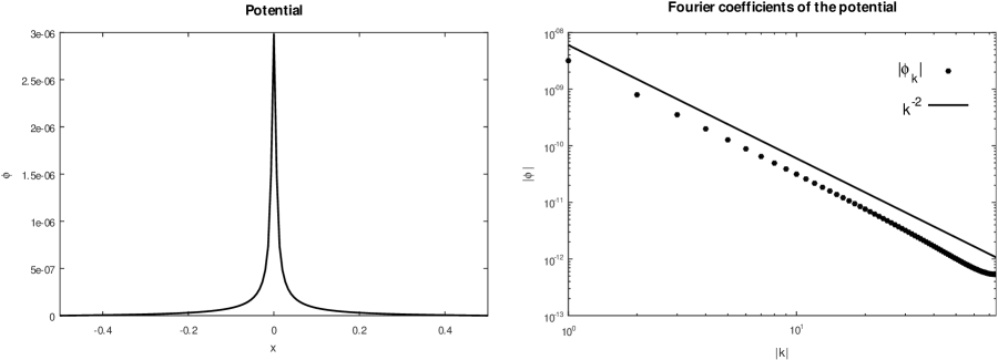
Figure 1. The graph of the regularized electrostatic potential $\phi_{num}(|x|)$ (left), and its Fourier transform $\hat{\phi}_{num}(\|\boldsymbol{k}\|)$ (right). The line $\|\boldsymbol{k}\|^{-2}$ is given for reference.

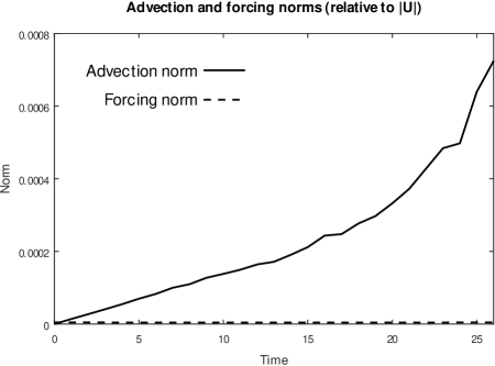
Figure 2. The time series of the quadratic norms of the advection part of (3.33) (solid line), and its potential forcing part (dashed line), for the electrostatic potential. Both norms are given relative to the norm of the turbulent velocity $\boldsymbol{u}$ itself.

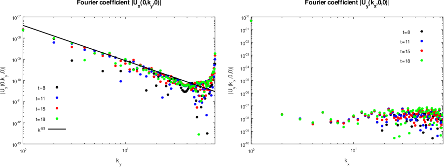
Figure 3. The values of $|\hat{u}_{x}(0,k_{y},0)|$ and $|\hat{u}_{y}(k_{x},0,0)|$ for the electrostatic potential forcing, captured at times $t=8,11,15,18$. The line $k_{y}^{-5/3}$ is given for the reference.

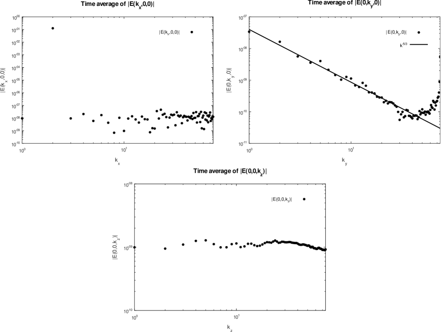
Figure 4. The values of $|\hat{E}(k_{x},0,0)|$, $|\hat{E}(0,k_{y},0)|$ and $|\hat{E}(0,0,k_{z})|$ for the electrostatic potential forcing, averaged between the times $t=8$ and $t=18$. The line $k_{y}^{-5/3}$ is given for the reference.

As mentioned above, in the absence of the potential forcing, the turbulent velocity equation in (3.33) is the decoupled (under the hydrostatic balance relation (3.19)) advection, differentiated once more in time (3.29). Thus, the laminar shear flow (4.1) would obviously be a steady state in such a situation, so we set the initial condition for the first time-derivative of the velocity to zero. This initial condition models the scenario where a potential forcing is introduced to an otherwise steady laminar shear flow.

Our first goal here is to locate the secular growth regime, which, in the absence of any sort of damping, should preclude the exponential growth and the resulting numerical blow-up. In order to do that, first we find that our numerical simulation blows up shortly after time $t=26$ units. To locate the regime with the secular growth, in Figure 2 we plot the quadratic norms of the advection and forcing terms in (3.33), relative to the norm of the velocity itself, as functions of time. Observe that, while the potential forcing norm remains close to a very small constant, the advection norm grows linearly with time until roughly 18-20 time units, after which a rapid, exponential growth starts. Thus, the secular growth regime in this scenario extends roughly until the time $t=18$ units.

Before proceeding to study the time averages of the Fourier transforms of the kinetic energy, we examine the snapshots of the Fourier transforms of the turbulent velocity. Now, observe that since, for a given time value, $\boldsymbol{u}(\boldsymbol{x})$ is a vector field, its Fourier transform $\hat{\boldsymbol{u}}(\boldsymbol{k})$ is also a vector field – namely, not only $\hat{\boldsymbol{u}}(\boldsymbol{k})$ consists of the three scalar components $\hat{u}_{x}(\boldsymbol{k})$, $\hat{u}_{y}(\boldsymbol{k})$ and $\hat{u}_{z}(\boldsymbol{k})$, but also each of these three components is a function of the three-dimensional wavevector $\boldsymbol{k}$. As a result, $\hat{\boldsymbol{u}}(\boldsymbol{k})$ may potentially have a complex structure in the full three-dimensional space, which would lead to an exhaustive study.

Thus, for the convenience of the reader, in the current work we restrict the presented results only to those which would be relatively easy to observe experimentally. In the literature [10, 22], the Fourier transforms are typically presented along a given direction, which suggests that the observed data are averaged over the other two directions, thus corresponding to zero Fourier wavenumbers. Thus, here we focus on the Fourier transforms $\hat{\boldsymbol{u}}(k_{x},0,0)$, $\hat{\boldsymbol{u}}(0,k_{y},0)$ and $\hat{\boldsymbol{u}}(0,0,k_{z})$, which are three-dimensional vector functions of a scalar argument. Further, we find that the majority of the components of these vector functions have typical values of the machine round-off errors, and thus appear to belong to the null space of the dynamics, for the given initial condition and the potential. Only the two components, $\hat{u}_{x}(0,k_{y},0)$ and $\hat{u}_{y}(k_{x},0,0)$, are discernibly nonzero.

In Figure 3, we show the snapshots of $|\hat{u}_{x}(0,k_{y},0)|$ and $|\hat{u}_{y}(k_{x},0,0)|$ at $t=8,11,15,18$, which belong to the regime of the secular growth. As we can see, although the component $|\hat{u}_{x}(0,k_{y},0)|$ shows noticeable scattering, the top of the scatterplot visibly decays as $k_{y}^{-5/3}$, which corresponds to the Kolmogorov spectrum. On the other hand, the component $\hat{u}_{y}(k_{x},0,0)$ exhibits a largely flat spectrum, with the exception of a single large scale value which corresponds to the shear flow (4.1).

The kinetic energy of the flow $E(\boldsymbol{x})=\|\boldsymbol{u}(\boldsymbol{x})\|^{2}/2$, as well as its Fourier transform $\hat{E}(\boldsymbol{k})$, are scalar functions of vector arguments, and thus it is relatively easy to examine the structure of the latter along the axes. In Figure 4 we present the time averages of $|\hat{E}(k_{x},0,0)|$, $|\hat{E}(0,k_{y},0)|$ and $|\hat{E}(0,0,k_{z})|$, computed between the times $t=8$ and $t=18$. Observe that, while the time averages of $|\hat{E}(k_{x},0,0)|$ and $|\hat{E}(0,0,k_{z})|$ have largely flat spectra, the time-average of $|\hat{E}(0,k_{y},0)|$ aligns very well with the reference line $k_{y}^{-5/3}$, which matches the Kolmogorov spectrum. This result agrees with the experiment of Buchhave and Velte [10], who also observed the Kolmogorov spectrum of the kinetic energy along the direction of the flow.

4.2. Gravity potential

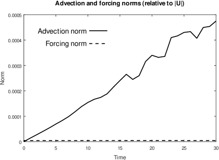
Figure 5. The time series of the quadratic norms of the advection part of (3.33) (solid line), and its potential forcing part (dashed line), for the gravity potential. Both norms are given relative to the norm of the turbulent velocity $\boldsymbol{u}$ itself.

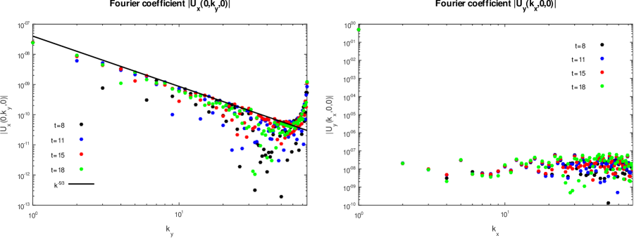
Figure 6. The values of $|\hat{u}_{x}(0,k_{y},0)|$ and $|\hat{u}_{y}(k_{x},0,0)|$ for the gravity potential forcing, captured at times $t=8,11,15,18$. The line $k_{y}^{-5/3}$ is given for the reference.

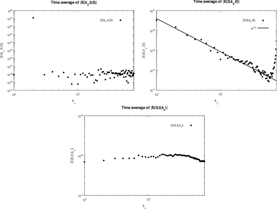
Figure 7. The values of $|\hat{E}(k_{x},0,0)|$, $|\hat{E}(0,k_{y},0)|$ and $|\hat{E}(0,0,k_{z})|$ for the gravity potential forcing, averaged between the times $t=8$ and $t=18$. The line $k_{y}^{-5/3}$ is given for the reference.

Here we repeat the simulations above with the same initial condition (4.1) for the gravity potential, which is obtained by inverting the sign of (4.4) with the same parameters. As a result, the plot of our gravity potential is a vertical mirror image of the electrostatic potential in Figure 1 with an identical decay of its respective Fourier transform, and thus we do not show it in a separate figure.

Following the same strategy as the one for the electrostatic potential above, here we attempt to identify the secular growth regime by numerically integrating (3.33) with the gravity potential until time $t=30$. Unlike the electrostatic potential, the gravity potential does not cause the exponential blow-up within the same time frame, however, as we show in Figure 5, the time series of the advection norm start developing oscillations by the time $t=18$-20 units. Thus, here we restrict the examination to the same time interval as above for the electrostatic potential, that is, up until $t=18$ units.

In Figure 6, we show the snapshots of $|\hat{u}_{x}(0,k_{y},0)|$ and $|\hat{u}_{y}(k_{x},0,0)|$ for the gravity potential forcing at the same times $t=8,11,15,18$ as above for the electrostatic potential. The general properties of the plots here are essentially the same as those for the electrostatic potential. The top values of the component $|\hat{u}_{x}(0,k_{y},0)|$ visibly decay as $k_{y}^{-5/3}$ (which corresponds to the Kolmogorov spectrum), whereas the component $\hat{u}_{y}(k_{x},0,0)$ exhibits a largely flat spectrum, with the exception of a single large scale value which corresponds to the shear flow (4.1).

In Figure 7 we present the time averages of $|\hat{E}(k_{x},0,0)|$, $|\hat{E}(0,k_{y},0)|$ and $|\hat{E}(0,0,k_{z})|$ for the gravity potential, computed between the times $t=8$ and $t=18$. The behavior of the time-averaged energy spectra is similar to those of the electrostatic potential above, namely, the time averages of $|\hat{E}(k_{x},0,0)|$ and $|\hat{E}(0,0,k_{z})|$ have largely flat spectra, while the time-average of $|\hat{E}(0,k_{y},0)|$ aligns very well with the reference line $k_{y}^{-5/3}$.

4.3. Thomas–Fermi potential

After observing the energy spectra for the electrostatic and gravitational potentials (which are the long-range potentials), it is interesting to look at what happens for some common short-range interatomic potentials. Here we examine the behavior of the flow for the same initial condition in (4.1), forced by the Thomas–Fermi potential with the Bohr screening function.

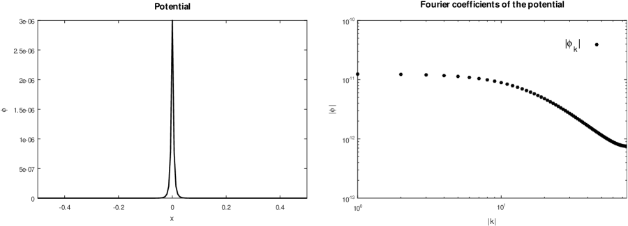
Figure 8. The graph of the regularized Thomas–Fermi potential with the Bohr screening function.

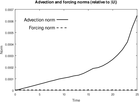
Figure 9. The time series of the quadratic norms of the advection part of (3.33) (solid line), and its potential forcing part (dashed line), for the Thomas–Fermi potential. Both norms are given relative to the norm of the turbulent velocity $\boldsymbol{u}$ itself.

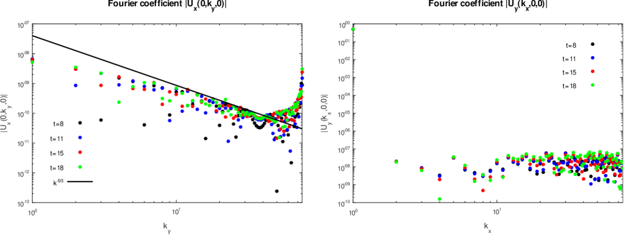
Figure 10. The values of $|\hat{u}_{x}(0,k_{y},0)|$ and $|\hat{u}_{y}(k_{x},0,0)|$ for the Thomas–Fermi potential forcing, captured at times $t=8,11,15,18$. The line $k_{y}^{-5/3}$ is given for the reference.

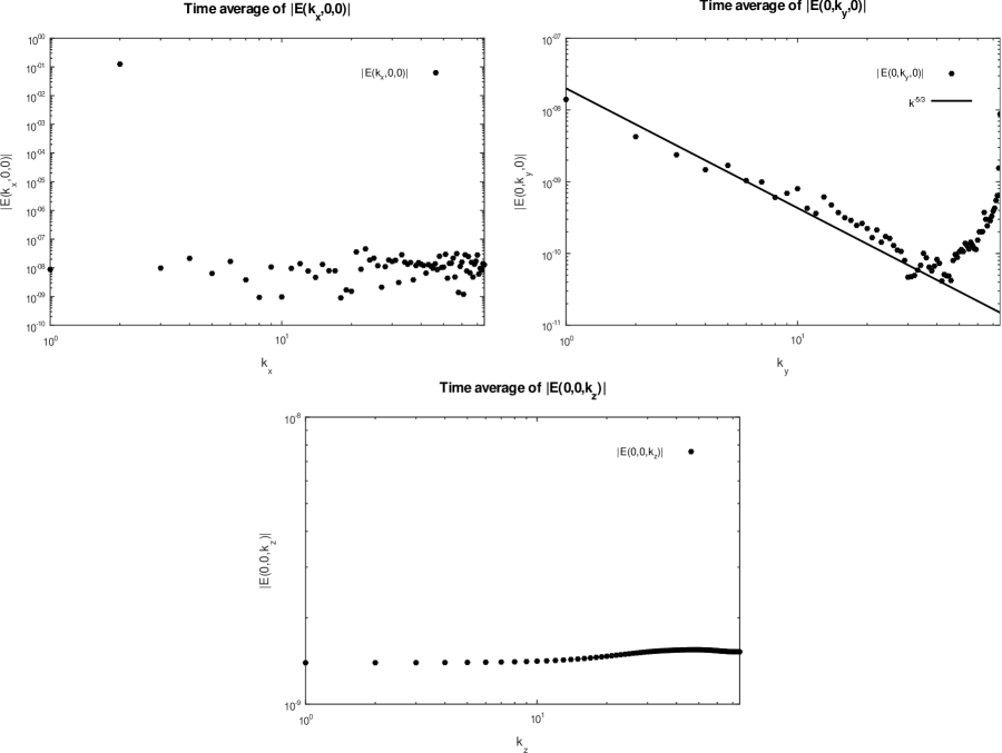
Figure 11. The values of $|\hat{E}(k_{x},0,0)|$, $|\hat{E}(0,k_{y},0)|$ and $|\hat{E}(0,0,k_{z})|$ for the Thomas–Fermi potential forcing, averaged between the times $t=8$ and $t=18$. The line $k_{y}^{-5/3}$ is given for the reference.

The Thomas–Fermi potential [30, 13] is given via

(4.5) $$\phi(r)=\frac{\phi_{0}}{r}\eta\left(\frac{r}{\sigma}\right),$$

where $\sigma$ is the Bohr radius of the potential, while $\eta(r)$ is the screening function. According to the Thomas–Fermi theory, $\eta(r)$ satisfies the Thomas–Fermi nonlinear differential equation, whose solution cannot be expressed in terms of elementary functions [28]. Thus, it is not unusual to choose $\eta(r)$ empirically instead (for example, by fitting to the scattering measurements, which results in the Ziegler–Biersack–Littmark potential [33]). Arguably, the simplest approximate screening function for the Thomas–Fermi potential was suggested by Bohr:

(4.6) $$\eta(r)=e^{-r}.$$

Since, in the current work, it is not our goal to accurately model the interactions between atoms, but rather to study the energy spectra for various potential types, here we study the properties of the solution of (3.33) with the same initial condition (4.1), forced by the Thomas–Fermi potential (4.5) with the Bohr screening function (4.6). The potential is regularized in the same way as in (4.2), that is, by capping it with the inverted parabola to avoid the singularity at zero. The parameters $\phi_{0}$ and $\sigma$ are chosen as follows:

(4.7) $$\phi_{0}=10^{-8},\qquad\sigma=10^{-2},$$

that is, the Bohr radius is two orders of magnitude smaller than the size of the domain. The resulting potential, together with its Fourier transform, is displayed in Figure 8. As we can see, the effective range of the Thomas–Fermi potential is visibly much shorter than that of the electrostatic and gravitational potentials, which is also confirmed by the relatively flat spectrum of its Fourier transform at large scales.

In this scenario, the numerical blow-up of the solution of (3.33) occurs shortly after the time $t=25$ units. In Figure 9, we show the time series of the advection and forcing norms up until the blow-up time. Observe that the linear growth of the advection norm ceases around the time $t=18$ units, and is replaced with an exponential growth leading to the blow-up, similarly to what happened for the electrostatic potential in Figure 2.

In Figure 10, we show the snapshots of $|\hat{u}_{x}(0,k_{y},0)|$ and $|\hat{u}_{y}(k_{x},0,0)|$ for the Thomas–Fermi potential forcing at the same times $t=8,11,15,18$ as above for the electrostatic potential. Observe that the shape of the Fourier transform of the potential appears to affect the top values of the component $|\hat{u}_{x}(0,k_{y},0)|$ – namely, the large scale components of the Fourier transform fall below the $k_{y}^{-5/3}$ line, while the small scale components are still aligned with it. The component $\hat{u}_{y}(k_{x},0,0)$ behaves in the same manner as before for the electrostatic and gravity potentials, exhibiting a largely flat spectrum, with the exception of a single large scale value which corresponds to the shear flow (4.1).

In Figure 11 we present the time averages of $|\hat{E}(k_{x},0,0)|$, $|\hat{E}(0,k_{y},0)|$ and $|\hat{E}(0,0,k_{z})|$ for the Thomas–Fermi potential, computed between the times $t=8$ and $t=18$. The behavior of the time-averaged energy spectra $|\hat{E}(k_{x},0,0)|$ and $|\hat{E}(0,0,k_{z})|$ is the same as that for the electrostatic and gravity potentials, that is, they are largely flat. Surprisingly, the time-average of $|\hat{E}(0,k_{y},0)|$ exhibits something resembling a “tiered” structure, where snippets of the spectrum visibly align with the reference line $k_{y}^{-5/3}$, with abrupt transitions in between. This is, however, different from what was observed for the electrostatic and gravity potentials, where almost the whole spectrum, except for very small scales, aligned consistently with the reference line.

4.4. Lennard-Jones potential

The second short-range interaction potential we examine here is an analog of the Lennard-Jones interatomic potential [21]. The chief difference between the Lennard-Jones potential and the Thomas–Fermi potential is that the former combines the attraction at longer distances with the repulsion at short distances.

Just as all preceding potentials, the Lennard-Jones potential has a singularity at zero. However, unlike the preceding potentials, the behavior of the Lennard-Jones potential leading to the singularity is much steeper ($r^{-12}$ versus $r^{-1}$), and, unfortunately, regularizing it with the inverted parabola, like we did above for the electrostatic, gravity and Thomas–Fermi potentials, does not work.

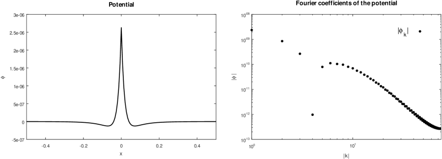
Figure 12. The graph of the model Lennard-Jones potential $\phi^{num}_{LJ}(|x|)$ (left), and its Fourier transform $\hat{\phi}^{num}_{LJ}(\|\boldsymbol{k}\|)$ (right).

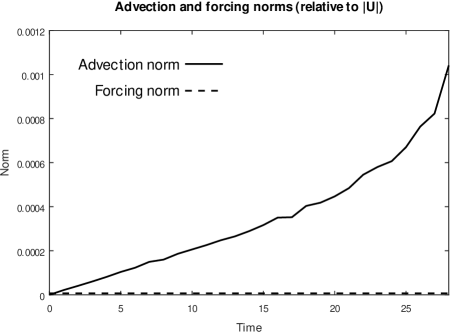
Figure 13. The time series of the quadratic norms of the advection part of (3.33) (solid line), and its potential forcing part (dashed line), for the Lennard-Jones potential. Both norms are given relative to the norm of the turbulent velocity $\boldsymbol{u}$ itself.

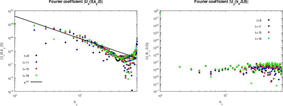
Figure 14. The values of $|\hat{u}_{x}(0,k_{y},0)|$ and $|\hat{u}_{y}(k_{x},0,0)|$ for the Lennard-Jones potential forcing, captured at times $t=8,11,15,18$. The line $k_{y}^{-5/3}$ is given for the reference.

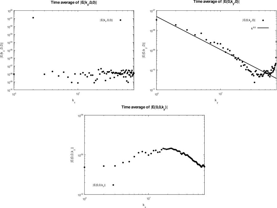
Figure 15. The values of $|\hat{E}(k_{x},0,0)|$, $|\hat{E}(0,k_{y},0)|$ and $|\hat{E}(0,0,k_{z})|$ for the Lennard-Jones potential forcing, averaged between the times $t=8$ and $t=18$. The line $k_{y}^{-5/3}$ is given for the reference.

Instead, we eliminate the singularity at zero by shifting the argument of the potential by a positive offset, so that the infinite value is never reached for a nonnegative argument. Namely, recall that the Lennard-Jones potential is given via

(4.8) $$\phi_{LJ}(r)=\phi_{0}\bigg{[}\left(\frac{\sigma}{r}\right)^{12}-\left(\frac{\sigma}{r}\right)^{6}\bigg{]}.$$

For the numerical simulations, we modify the above expression as follows:

(4.9) $$\phi_{LJ}^{num}(r)=\phi_{LJ}(r+r_{0}),\qquad r_{0}>0.$$

The potential thus becomes shifted to the left along the horizontal axis, such that the infinity is achieved for a negative value of the argument. However, since the distance between the particles cannot be negative, the expression above is finite at any model discretization point.

For the simulation, we use the following values of the parameters:

(4.10) $$\phi_{0}=10^{-6},\qquad\sigma=0.25,\qquad r_{0}=0.21.$$

The graph of the model potential, together with its Fourier transform, is shown in Figure 12. Observe that the model potential indeed combines the attraction at longer distances with the repulsion at short distances, just as intended.

For the Lennard-Jones potential, the numerical blow-up of the solution of (3.33) occurs shortly after the time $t=28$ units. In Figure 13, we show the time series of the advection and forcing norms of the numerical solution of (3.33) for the Lennard-Jones potential up until the blow-up time. Observe that the linear growth of the advection norm ceases around the time $t=20$ units, and is replaced with an exponential growth leading to the blow-up.

In Figure 14, we show the snapshots of $|\hat{u}_{x}(0,k_{y},0)|$ and $|\hat{u}_{y}(k_{x},0,0)|$ for the Lennard-Jones potential forcing at the same times $t=8,11,15,18$ as for all of the preceding cases. Observe that the shape of the Fourier transform of the potential also affects the top values of the component $|\hat{u}_{x}(0,k_{y},0)|$ (just as for the Thomas–Fermi potential above) – namely, the large scale components of the Fourier transform fall below the $k_{y}^{-5/3}$ line, while the small scale components are still aligned with it. The component $\hat{u}_{y}(k_{x},0,0)$ behaves in the same manner as before for the electrostatic, gravity and Thomas–Fermi potentials, exhibiting a largely flat spectrum, with the exception of a single large scale value which corresponds to the shear flow (4.1).

In Figure 15 we present the time averages of $|\hat{E}(k_{x},0,0)|$, $|\hat{E}(0,k_{y},0)|$ and $|\hat{E}(0,0,k_{z})|$ for the Lennard-Jones potential, computed between the times $t=8$ and $t=18$. The behavior of the time-averaged energy spectra $|\hat{E}(k_{x},0,0)|$ and $|\hat{E}(0,0,k_{z})|$ resembles that for the electrostatic, gravity and Thomas–Fermi potentials, that is, the spectra do not exhibit any systematic power decay. The scaling of time-average of $|\hat{E}(0,k_{y},0)|$, on the other hand, clearly follows the reference line $k_{y}^{-5/3}$.

4.5. Large scale potential (Vlasov equation)

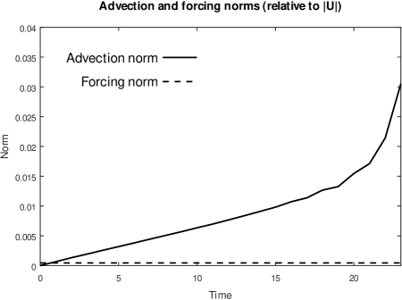
Figure 16. The time series of the quadratic norms of the advection part of (3.33) (solid line), and its potential forcing part (dashed line), for the large scale potential. Both norms are given relative to the norm of the turbulent velocity $\boldsymbol{u}$ itself.

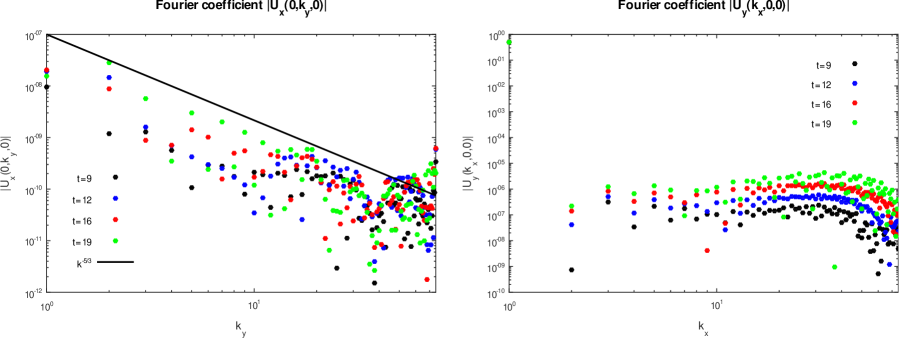
Figure 17. The values of $|\hat{u}_{x}(0,k_{y},0)|$ and $|\hat{u}_{y}(k_{x},0,0)|$ for the large scale potential forcing, captured at times $t=9,12,16,19$. The line $k_{y}^{-5/3}$ is given for the reference.

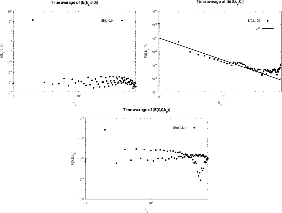
Figure 18. The values of $|\hat{E}(k_{x},0,0)|$, $|\hat{E}(0,k_{y},0)|$ and $|\hat{E}(0,0,k_{z})|$ for the large scale potential forcing, averaged between the times $t=9$ and $t=19$. The line $k_{y}^{-5/3}$ is given for the reference.

So far, we examined the dynamics of the turbulent velocity equation (3.33) for a short-range interatomic potential (such as Thomas–Fermi or Lennard-Jones), or a “rangeless” potential, such as electrostatic or gravitational. In all cases, we observed the kinetic energy spectra consistent with the Kolmogorov power decay. The only scenario which remains unexamined is the one where the potential is confined solely to large scales, in the context of the Vlasov equation (2.22) for a single particle.

In the current work, we examine our hypothesis of formation of turbulence in (3.33) by potentials of different types, and it is not our goal to accurately reproduce the actual compressible gas flow with proper relations between the density, velocity, and other variables. Therefore, here it suffices to set the potential $\phi$ in (3.33) to a simple, artificial combination of the large scale periodic functions:

(4.11) $$\phi(x,y,z)=\phi_{0}\cos(2\pi x)\sin(2\pi y)\cos(2\pi z).$$

For our simulation, we set $\phi_{0}=10^{-5}$, which yields the secular rate of growth similar to the potentials tested above. In this scenario, the numerical blow-up occurs shortly after the time $t=24$ units. In Figure 16, we show the time series of the advection and forcing norms of the numerical solution of (3.33) for the large scale potential up until the blow-up time. Observe that the linear growth of the advection norm ceases around the time $t=20$ units, and is replaced with the exponential growth leading to the blow-up.

In Figure 17, we show the snapshots of $|\hat{u}_{x}(0,k_{y},0)|$ and $|\hat{u}_{y}(k_{x},0,0)|$ for the large scale potential forcing at the times $t=9,12,16,19$. Here, the velocity Fourier transform $|\hat{u}_{x}(0,k_{y},0)|$ follows the $k_{y}^{-5/3}$ reference line rather poorly, as one can discern only the general “bulk” trend corresponding to the Kolmogorov decay, but not the “sharp top” as for the electrostatic or gravity potentials above. The component $\hat{u}_{y}(k_{x},0,0)$ behaves in the same manner as before for the electrostatic, gravity, Thomas–Fermi and Lennard-Jones potentials, exhibiting a largely flat spectrum, with the exception of a single large scale value which corresponds to the shear flow (4.1).

In Figure 18 we present the time averages of $|\hat{E}(k_{x},0,0)|$, $|\hat{E}(0,k_{y},0)|$ and $|\hat{E}(0,0,k_{z})|$ for the large scale potential, computed between the times $t=9$ and $t=19$. The behavior of the time-averaged energy spectra $|\hat{E}(k_{x},0,0)|$ and $|\hat{E}(0,0,k_{z})|$ is the same as that for the electrostatic, gravity, Thomas–Fermi and Lennard-Jones potentials, that is, they are largely flat. Remarkably, the scaling of the time-average of $|\hat{E}(0,k_{y},0)|$ follows the reference line $k_{y}^{-5/3}$ almost as accurately as for the electrostatic and gravitational potentials, and notably better than for the Thomas–Fermi and Lennard-Jones potentials.

Concluding this section, we note that the bulk decay properties of the kinetic energy spectrum along the direction of the large scale shear flow depend rather weakly on the type of the potential overall, and tend to support the Kolmogorov spectrum hypothesis for the whole variety of studied potentials.

5. Summary

In the current work, we study the ability of the potential interaction between particles to form turbulent structures with power decay spectra from an initially laminar shear flow. We start with a simple model consisting of only two particles, which interact via a potential. We then change the variables to those which quantify the motion of the center of mass of the system (the mean flow), and the difference of the coordinates of the particles (the turbulent variables), and formulate the Liouville equation for the turbulent coordinate and velocity variables. Alternatively, we formulate the Vlasov equation for one of the particles in the pair, by excluding the other particle via a simple closure.

Observing that these Liouville and Vlasov equations have the same form (differing only in the type of the forcing potential), we derive the hierarchy of the velocity moment transport equations for either of the two in the same manner as in the conventional fluid mechanics. Due to the fact that this hierarchy lacks the Boltzmann collision integral (which is replaced by the potential forcing), we introduce a novel closure, based upon the condition of a high Reynolds number of the flow. Our closure leads to a standalone equation for the velocity variable, forced by the interaction potential.

As the turbulent velocity equation is a nonlinear second-order PDE, we study the behavior of its solutions via numerical simulations, using a large scale laminar shear flow as the initial condition. We examine the resulting dynamics for the following interaction potentials: electrostatic, gravitational, Thomas–Fermi, Lennard-Jones, as well as the Vlasov-type large scale mean field potential. In each scenario, we discover the regime of secular growth which precludes the exponential blow-up, where the latter apparently occurs due to the lack of dissipation. In all scenarios, the time-averaged kinetic energy of the flow in this secular growth regime decays as the negative five-thirds power of its Fourier wavenumber, which corresponds to the Kolmogorov turbulence spectrum.

While the initial examination of the formation of turbulence, according to our hypothesis, has been completed in the present work, the properties of turbulence dissipation are still inaccessible in the current state of our model. The reason for this is that, in its present form, the turbulent velocity equation itself lacks dissipation. This, in turn, stems from the fact that there is no dissipation in the simple two-particle model we study here – the sole interaction present in the system occurs via a potential, and is, therefore, fully time-reversible. In order to introduce dissipation, a promising approach seems to be to take the multiparticle system as a starting point, and treat the collisions of the particles beyond the first two as irreversible [2]. We will explore this approach in the future work.

Acknowledgment

This work was supported by the Simons Foundation grant #636144.

Appendix A Multiparticle dynamics

Here, we consider a dynamical system which consists of $N$ identical particles, interacting via a potential $\phi(r)$. Denoting the coordinate and velocity of the $i$-th particle via $\boldsymbol{x}_{i}$ and $\boldsymbol{v}_{i}$, respectively, we have the following system of equations of motion:

(A.1) $$\frac{\mathrm{d}\boldsymbol{x}_{i}}{\mathrm{d}t}=\boldsymbol{v}_{i},\qquad\frac{\mathrm{d}\boldsymbol{v}_{i}}{\mathrm{d}t}=-\sum_{\genfrac{}{}{0.0pt}{}{j=1}{j\neq i}}^{N}\frac{\partial}{\partial\boldsymbol{x}_{i}}\phi(\|\boldsymbol{x}_{i}-\boldsymbol{x}_{j}\|).$$

The total momentum and energy of all particles are preserved by the dynamics:

(A.2) $$\sum_{i=1}^{N}\boldsymbol{v}_{i}=\text{const},\qquad\sum_{i=1}^{N}\frac{\|\boldsymbol{v}\|^{2}}{2}+\sum_{i=1}^{N-1}\sum_{j=i+1}^{N}\phi(\|\boldsymbol{x}_{i}-\boldsymbol{x}_{j}\|)=\text{const}.$$

Observe that, for a given value of the momentum, it is always possible to choose the inertial reference frame in which the momentum becomes zero; thus, without much loss of generality, we will further assume that the total momentum of the system is zero.

Following our work [3], we concatenate the coordinates as $\boldsymbol{X}=(\boldsymbol{x}_{1},\ldots,\boldsymbol{x}_{N})$, and velocities as $\boldsymbol{V}=(\boldsymbol{v}_{1},\ldots,\boldsymbol{v}_{N})$. In these notations, we can write

(A.3) $$\frac{\mathrm{d}\boldsymbol{X}}{\mathrm{d}t}=\boldsymbol{V},\qquad\frac{\mathrm{d}\boldsymbol{V}}{\mathrm{d}t}=-\frac{\partial\Phi}{\partial\boldsymbol{X}},\qquad\Phi(\boldsymbol{X})=\sum_{i=1}^{N-1}\sum_{j=i+1}^{N}\phi(\|\boldsymbol{x}_{i}-\boldsymbol{x}_{j}\|).$$

In the variables $\boldsymbol{X}$ and $\boldsymbol{V}$, the conservation of the energy can be expressed via

(A.4) $$\|\boldsymbol{V}\|^{2}+2\Phi(\boldsymbol{X})=\text{const}.$$

Let $F(t,\boldsymbol{X},\boldsymbol{V})$ be the density of states of the dynamical system above. Then, the Liouville equation for $F$ is given via

(A.5) $$\frac{\partial F}{\partial t}+\boldsymbol{V}\cdot\frac{\partial F}{\partial\boldsymbol{X}}=\frac{\partial\Phi}{\partial\boldsymbol{X}}\cdot\frac{\partial F}{\partial\boldsymbol{V}}.$$

Any suitable $F_{0}$ of the form

(A.6) $$F_{0}(\boldsymbol{X},\boldsymbol{V})=F_{0}\big{(}\|\boldsymbol{V}\|^{2}+2\Phi(\boldsymbol{X})\big{)}$$

is a steady state for (A.5). Among those, the canonical Gibbs state is

(A.7) $$F_{G}(\boldsymbol{X},\boldsymbol{V})=\frac{1}{(2\pi\theta_{0})^{3N/2}Z_{N}}\exp\left(-\frac{\|\boldsymbol{V}\|^{2}+2\Phi(\boldsymbol{X})}{2\theta_{0}}\right),\qquad Z_{N}=\int e^{-\Phi(\boldsymbol{X})/\theta_{0}}\>\!\mathrm{d}\boldsymbol{X},$$

where $\theta_{0}$ is the kinetic temperature. The conservation of the Rényi divergences is shown in the same manner as in Section 2; indeed, for $\psi_{1}(F)$ and $\psi_{2}(F)$ we have

(A.8) $$\frac{\partial}{\partial t}\int\psi_{1}(F)\psi_{2}(F_{0})\>\!\mathrm{d}\boldsymbol{X}\>\!\mathrm{d}\boldsymbol{V}=\int\psi_{2}(F_{0})\frac{\partial\psi_{1}(F)}{\partial t}\>\!\mathrm{d}\boldsymbol{X}\>\!\mathrm{d}\boldsymbol{V}=\int\psi_{2}(F_{0})\bigg{(}\frac{\partial\Phi}{\partial\boldsymbol{X}}\cdot\frac{\partial\psi_{1}(F)}{\partial\boldsymbol{V}}-\\ -\boldsymbol{V}\cdot\frac{\partial\psi_{1}(F)}{\partial\boldsymbol{X}}\bigg{)}\>\!\mathrm{d}\boldsymbol{X}\>\!\mathrm{d}\boldsymbol{V}=\int\psi_{1}(F)\bigg{(}\boldsymbol{V}\cdot\frac{\partial\psi_{2}(F_{0})}{\partial\boldsymbol{X}}-\frac{\partial\Phi}{\partial\boldsymbol{X}}\cdot\frac{\partial\psi_{2}(F_{0})}{\partial\boldsymbol{V}}\bigg{)}\>\!\mathrm{d}\boldsymbol{X}\>\!\mathrm{d}\boldsymbol{V}=0.$$

A.1. Marginal distributions of the Gibbs state

For the particles $1,\ldots,k$, $k\leq N$, we have

(A.9) $$F^{(1,\ldots,k)}_{G}=\int F_{G}(\boldsymbol{X},\boldsymbol{V})\>\!\mathrm{d}\boldsymbol{x}_{k+1}\>\!\mathrm{d}\boldsymbol{v}_{k+1}\ldots\>\!\mathrm{d}\boldsymbol{x}_{N}\>\!\mathrm{d}\boldsymbol{v}_{N}=\\ =\frac{1}{(2\pi\theta_{0})^{3k/2}}e^{-(\|\boldsymbol{v}_{1}\|^{2}+\ldots+\|\boldsymbol{v}_{k}\|^{2})/2\theta_{0}}\prod_{i=1}^{k-1}\prod_{j=i+1}^{k}e^{-\phi(\|\boldsymbol{x}_{i}-\boldsymbol{x}_{j}\|)/\theta_{0}}Y^{(k)}(\boldsymbol{x}_{1},\ldots,\boldsymbol{x}_{k}),$$

where $Y^{(k)}_{N}$ is a multiple of the $k$-particle cavity distribution function [9]:

(A.10) $$Y^{(k)}_{N}(\boldsymbol{x}_{1},\ldots,\boldsymbol{x}_{k})=\frac{1}{Z_{N}}\int\bigg{(}\prod_{i=k+1}^{N}e^{-(\phi(\|\boldsymbol{x}_{1}-\boldsymbol{x}_{i}\|)+\ldots+\phi(\|\boldsymbol{x}_{k}-\boldsymbol{x}_{i}\|))/\theta_{0}}\\ \prod_{j=i+1}^{N}e^{-\phi(\|\boldsymbol{x}_{i}-\boldsymbol{x}_{j}\|)/\theta_{0}}\bigg{)}\>\!\mathrm{d}\boldsymbol{x}_{k+1}\ldots\>\!\mathrm{d}\boldsymbol{x}_{N}.$$

For the two and three particles, we can write their marginal distributions $F_{G}^{(1,2)}$ and $F_{G}^{(1,2,3)}$ via

(A.11a) $$F_{G}^{(1,2)}=\frac{1}{(2\pi\theta_{0})^{3/2}V}e^{-\|\boldsymbol{v}_{1}\|^{2}/2\theta_{0}}\frac{1}{(2\pi\theta_{0})^{3/2}V}e^{-\|\boldsymbol{v}_{2}\|^{2}/2\theta_{0}}e^{-\phi(\|\boldsymbol{x}_{2}-\boldsymbol{x}_{1}\|)/\theta_{0}}\\ V^{2}Y^{(2)}(\boldsymbol{x}_{1},\boldsymbol{x}_{2})=F_{G}^{(1)}(\boldsymbol{v}_{1})F_{G}^{(2)}(\boldsymbol{v}_{2})e^{-\phi(\|\boldsymbol{x}_{2}-\boldsymbol{x}_{1}\|)/\theta_{0}}V^{2}Y^{(2)}(\boldsymbol{x}_{1},\boldsymbol{x}_{2}),$$

(A.11b) $$F_{G}^{(1,2,3)}=\frac{1}{(2\pi\theta_{0})^{3}}e^{-(\|\boldsymbol{v}_{1}\|^{2}+\|\boldsymbol{v}_{2}\|^{2})/2\theta_{0}}\frac{1}{Z_{2}}e^{-\phi(\|\boldsymbol{x}_{2}-\boldsymbol{x}_{1}\|)/\theta_{0}}\frac{1}{(2\pi\theta_{0})^{3/2}V}e^{-\|\boldsymbol{v}_{3}\|^{2}/2\theta_{0}}\\ Z_{2}Ve^{-(\phi(\|\boldsymbol{x}_{3}-\boldsymbol{x}_{1}\|)+\phi(\|\boldsymbol{x}_{3}-\boldsymbol{x}_{2}\|))/\theta_{0}}Y^{(3)}_{N}(\boldsymbol{x}_{1},\boldsymbol{x}_{2},\boldsymbol{x}_{3})=\\ =F_{G}^{(1,2)}(\boldsymbol{x}_{1},\boldsymbol{v}_{1},\boldsymbol{x}_{2},\boldsymbol{v}_{2})F_{G}^{(3)}(\boldsymbol{v}_{3})e^{-(\phi(\|\boldsymbol{x}_{3}-\boldsymbol{x}_{1}\|)+\phi(\|\boldsymbol{x}_{3}-\boldsymbol{x}_{2}\|))/\theta_{0}}Z_{2}VY^{(3)}_{N}(\boldsymbol{x}_{1},\boldsymbol{x}_{2},\boldsymbol{x}_{3}).$$

If the gas is dilute (that is, at average distances the particles are weakly affected by the potential interaction), then $V^{2}Y^{(2)}\to 1$, $Z_{2}VY^{(3)}\to 1$, and $F_{G}^{(1,2)}$, $F_{G}^{(1,2,3)}$ become

(A.12a) $$F_{G}^{(1,2)}=F_{G}^{(1)}(\boldsymbol{v}_{1})F_{G}^{(2)}(\boldsymbol{v}_{2})e^{-\phi(\|\boldsymbol{x}_{2}-\boldsymbol{x}_{1}\|)/\theta_{0}},$$

(A.12b) $$F_{G}^{(1,2,3)}=F_{G}^{(1,2)}(\boldsymbol{x}_{1},\boldsymbol{v}_{1},\boldsymbol{x}_{2},\boldsymbol{v}_{2})F_{G}^{(3)}(\boldsymbol{v}_{3})e^{-(\phi(\|\boldsymbol{x}_{3}-\boldsymbol{x}_{1}\|)+\phi(\|\boldsymbol{x}_{3}-\boldsymbol{x}_{2}\|))/\theta_{0}}.$$

Appendix B The closure for a single particle (Vlasov equation)

Here, we isolate a single particle (say, #1), and examine the transport of its marginal distribution $F^{(1)}$, given via

(B.1) $$F^{(1)}(t,\boldsymbol{x}_{1},\boldsymbol{v}_{1})=\int F(t,\boldsymbol{X},\boldsymbol{V})\>\!\mathrm{d}\boldsymbol{x}_{2}\>\!\mathrm{d}\boldsymbol{v}_{2}\ldots\>\!\mathrm{d}\boldsymbol{x}_{N}\>\!\mathrm{d}\boldsymbol{v}_{N}.$$

Integrating the Liouville equation in (A.5) over all particles but the first one, in the absence of boundary effects we arrive at

(B.2) $$\frac{\partial F^{(1)}}{\partial t}+\boldsymbol{v}_{1}\cdot\frac{\partial F^{(1)}}{\partial\boldsymbol{x}_{1}}=\sum_{i=2}^{N}\int\frac{\partial}{\partial\boldsymbol{x}_{1}}\phi(\|\boldsymbol{y}-\boldsymbol{x}_{1}\|)\cdot\frac{\partial}{\partial\boldsymbol{v}_{1}}F^{(1,i)}(\boldsymbol{x}_{1},\boldsymbol{v}_{1},\boldsymbol{y},\boldsymbol{w})\>\!\mathrm{d}\boldsymbol{y}\>\!\mathrm{d}\boldsymbol{w}.$$

Assuming that the gas is dilute, and the state $F$ is close to the Gibbs equilibrium, we use the same closure for $F^{(1,i)}$ as in (A.12a):

(B.3) $$F^{(1,i)}(\boldsymbol{x}_{1},\boldsymbol{v}_{1},\boldsymbol{y},\boldsymbol{w})=F^{(1)}(\boldsymbol{x}_{1},\boldsymbol{v}_{1})F^{(i)}(\boldsymbol{y},\boldsymbol{w})e^{-\phi(\|\boldsymbol{y}-\boldsymbol{x}_{1}\|)/\theta_{0}}.$$

This leads to

(B.4) $$\int\frac{\partial}{\partial\boldsymbol{x}_{1}}\phi(\|\boldsymbol{y}-\boldsymbol{x}_{1}\|)\cdot\frac{\partial}{\partial\boldsymbol{v}_{1}}F^{(1,i)}(\boldsymbol{x}_{1},\boldsymbol{v}_{1},\boldsymbol{y},\boldsymbol{w})\>\!\mathrm{d}\boldsymbol{y}\>\!\mathrm{d}\boldsymbol{w}=\frac{\partial}{\partial\boldsymbol{v}_{1}}F^{(1)}(\boldsymbol{x}_{1},\boldsymbol{v}_{1})\cdot\\ \cdot\int\frac{\partial}{\partial\boldsymbol{x}_{1}}\phi(\|\boldsymbol{y}-\boldsymbol{x}_{1}\|)e^{-\phi(\|\boldsymbol{y}-\boldsymbol{x}_{1}\|)/\theta_{0}}F^{(i)}(\boldsymbol{y},\boldsymbol{w})\>\!\mathrm{d}\boldsymbol{y}\>\!\mathrm{d}\boldsymbol{w}=\frac{\partial\bar{\phi}_{i}(\boldsymbol{x}_{1})}{\partial\boldsymbol{x}_{1}}\cdot\frac{\partial F^{(1)}}{\partial\boldsymbol{v}_{1}},$$

where

(B.5) $$\bar{\phi}_{i}(\boldsymbol{x})=-\theta_{0}\int e^{-\phi(\|\boldsymbol{x}-\boldsymbol{y}\|)/\theta_{0}}\rho_{i}(\boldsymbol{y})\>\!\mathrm{d}\boldsymbol{y},\qquad\rho_{i}(\boldsymbol{y})=\int F^{(i)}(\boldsymbol{y},\boldsymbol{w})\>\!\mathrm{d}\boldsymbol{w}.$$

Now, denoting

(B.6) $$\bar{\phi}(\boldsymbol{x})=\sum_{i=2}^{N}\bar{\phi}_{i}(\boldsymbol{x}),$$

we arrive at the Vlasov equation

(B.7) $$\frac{\partial F^{(1)}}{\partial t}+\boldsymbol{v}_{1}\cdot\frac{\partial F^{(1)}}{\partial\boldsymbol{x}_{1}}=\frac{\partial\bar{\phi}(\boldsymbol{x}_{1})}{\partial\boldsymbol{x}_{1}}\cdot\frac{\partial F^{(1)}}{\partial\boldsymbol{v}_{1}}.$$

This equation has the same structure as (2.13) and (2.22). Just as in (2.22), the potential $\bar{\phi}$ is, generally, time-dependent.

Appendix C The closure for a pair of particles

Here, we isolate a pair of particles (say, #1 and #2), and examine the transport of their marginal distribution $F^{(1,2)}$, given via

(C.1) $$F^{(1,2)}(t,\boldsymbol{x}_{1},\boldsymbol{v}_{1},\boldsymbol{x}_{2},\boldsymbol{v}_{2})=\int F(t,\boldsymbol{X},\boldsymbol{V})\>\!\mathrm{d}\boldsymbol{x}_{3}\>\!\mathrm{d}\boldsymbol{v}_{3}\ldots\>\!\mathrm{d}\boldsymbol{x}_{N}\>\!\mathrm{d}\boldsymbol{v}_{N}.$$

Integrating the Liouville equation in (A.5) over all particles but the first two, and assuming the absence of any boundary effects, we arrive at

(C.2) $$\bigg{(}\frac{\partial}{\partial t}+\boldsymbol{v}_{1}\cdot\frac{\partial}{\partial\boldsymbol{x}_{1}}+\boldsymbol{v}_{2}\cdot\frac{\partial}{\partial\boldsymbol{x}_{2}}\bigg{)}F^{(1,2)}=\int\bigg{(}\frac{\partial\Phi}{\partial\boldsymbol{x}_{1}}\cdot\frac{\partial}{\partial\boldsymbol{v}_{1}}+\frac{\partial\Phi}{\partial\boldsymbol{x}_{2}}\cdot\frac{\partial}{\partial\boldsymbol{v}_{2}}\bigg{)}F\>\!\mathrm{d}\boldsymbol{x}_{3}\>\!\mathrm{d}\boldsymbol{v}_{3}\ldots\>\!\mathrm{d}\boldsymbol{x}_{N}\>\!\mathrm{d}\boldsymbol{v}_{N},$$

where the terms with the derivatives in $\boldsymbol{v}_{i}$, $i>2$, are integrated out. Above, observe that the derivatives of the potential can be written via

(C.3a) $$\frac{\partial\Phi}{\partial\boldsymbol{x}_{1}}=-\phi^{\prime}(\|\boldsymbol{x}_{2}-\boldsymbol{x}_{1}\|)\frac{\boldsymbol{x}_{2}-\boldsymbol{x}_{1}}{\|\boldsymbol{x}_{2}-\boldsymbol{x}_{1}\|}+\sum_{i=3}^{N}\frac{\partial}{\partial\boldsymbol{x}_{1}}\phi(\|\boldsymbol{x}_{i}-\boldsymbol{x}_{1}\|),$$

(C.3b) $$\frac{\partial\Phi}{\partial\boldsymbol{x}_{2}}=\phi^{\prime}(\|\boldsymbol{x}_{2}-\boldsymbol{x}_{1}\|)\frac{\boldsymbol{x}_{2}-\boldsymbol{x}_{1}}{\|\boldsymbol{x}_{2}-\boldsymbol{x}_{1}\|}+\sum_{i=3}^{N}\frac{\partial}{\partial\boldsymbol{x}_{2}}\phi(\|\boldsymbol{x}_{i}-\boldsymbol{x}_{2}\|),$$

which allows to write the transport equation for $F^{(1,2)}$ via

(C.4) $$\bigg{(}\frac{\partial}{\partial t}+\boldsymbol{v}_{1}\cdot\frac{\partial}{\partial\boldsymbol{x}_{1}}+\boldsymbol{v}_{2}\cdot\frac{\partial}{\partial\boldsymbol{x}_{2}}\bigg{)}F^{(1,2)}=\phi^{\prime}(\|\boldsymbol{x}_{2}-\boldsymbol{x}_{1}\|)\frac{\boldsymbol{x}_{2}-\boldsymbol{x}_{1}}{\|\boldsymbol{x}_{2}-\boldsymbol{x}_{1}\|}\cdot\bigg{(}\frac{\partial}{\partial\boldsymbol{v}_{2}}-\frac{\partial}{\partial\boldsymbol{v}_{1}}\bigg{)}F^{(1,2)}+\\ +\sum_{i=3}^{N}\int\bigg{(}\frac{\partial}{\partial\boldsymbol{x}_{1}}\phi(\|\boldsymbol{x}_{i}-\boldsymbol{x}_{1}\|)\cdot\frac{\partial}{\partial\boldsymbol{v}_{1}}+\frac{\partial}{\partial\boldsymbol{x}_{2}}\phi(\|\boldsymbol{x}_{i}-\boldsymbol{x}_{2}\|)\cdot\frac{\partial}{\partial\boldsymbol{v}_{2}}\bigg{)}F^{(1,2,i)}\>\!\mathrm{d}\boldsymbol{x}_{i}\>\!\mathrm{d}\boldsymbol{v}_{i},$$

where $F^{(1,2,i)}$ is the marginal distribution of the three particles – the first, second, and $i$-th. The equation for the marginals in (C.4) is a part of the Bogoliubov–Born–Green–Kirkwood–Yvon hierarchy [6, 8, 16].

In order to proceed further, we need to introduce a closure for $F^{(1,2,i)}$. In similar scenarios in the literature [11, 12] it is assumed that the marginal distributions for different particles are independent; however, in the present context such an assumption would obviously be incorrect, which is indicated by the structure of $F_{0}$ in (A.7). Instead, here we follow our earlier work [2] and assume that the structure of $F^{(1,2,i)}$ mimics that of the corresponding three-particle marginal of $F_{G}$ in (A.12b); namely, $F^{(1,2,i)}$ has the form

(C.5) $$F^{(1,2,i)}(\boldsymbol{x}_{1},\boldsymbol{v}_{1},\boldsymbol{x}_{2},\boldsymbol{v}_{2},\boldsymbol{x}_{i},\boldsymbol{v}_{i})=F^{(1,2)}(\boldsymbol{x}_{1},\boldsymbol{v}_{1},\boldsymbol{x}_{2},\boldsymbol{v}_{2})F^{(i)}(\boldsymbol{x}_{i},\boldsymbol{v}_{i})e^{-(\phi(\|\boldsymbol{x}_{i}-\boldsymbol{x}_{1}\|)+\phi(\|\boldsymbol{x}_{i}-\boldsymbol{x}_{2}\|))/\theta_{0}},$$

where $F^{(i)}$ is the single-particle marginal distribution for the $i$-th particle. Observe that the closure in (C.5) becomes exact if $F$ is the steady state (A.7). Under this assumption, we arrive at

(C.6) $$\sum_{i=3}^{N}\int\bigg{(}\frac{\partial}{\partial\boldsymbol{x}_{1}}\phi(\|\boldsymbol{x}_{i}-\boldsymbol{x}_{1}\|)\cdot\frac{\partial}{\partial\boldsymbol{v}_{1}}+\frac{\partial}{\partial\boldsymbol{x}_{2}}\phi(\|\boldsymbol{x}_{i}-\boldsymbol{x}_{2}\|)\cdot\frac{\partial}{\partial\boldsymbol{v}_{2}}\bigg{)}F^{(1,2,i)}\>\!\mathrm{d}\boldsymbol{x}_{i}\>\!\mathrm{d}\boldsymbol{v}_{i}=\\ =\bigg{(}\frac{\partial F^{(1,2)}}{\partial\boldsymbol{v}_{1}}\cdot\frac{\partial}{\partial\boldsymbol{x}_{1}}+\frac{\partial F^{(1,2)}}{\partial\boldsymbol{v}_{2}}\cdot\frac{\partial}{\partial\boldsymbol{x}_{2}}\bigg{)}\bigg{(}-(N-2)\theta_{0}\int e^{-(\phi(\|\boldsymbol{x}_{1}-\boldsymbol{z}\|)+\phi(\|\boldsymbol{x}_{2}-\boldsymbol{z}\|))/\theta_{0}}\bar{\rho}(\boldsymbol{z})\>\!\mathrm{d}\boldsymbol{z}\bigg{)},$$

where we denote

(C.7) $$\bar{\rho}(\boldsymbol{z})=\frac{1}{N-2}\sum_{i=3}^{N}\rho_{i}(\boldsymbol{z}).$$

The transport equation for $F^{(1,2)}$ is now closed. Next, let us switch to the variables $\boldsymbol{x}$, $\boldsymbol{v}$, $\boldsymbol{y}$ and $\boldsymbol{w}$ from (2.10). In these variables, the closure term becomes

(C.8) $$-(N-2)\theta_{0}\int e^{-(\phi(\|\boldsymbol{x}_{1}-\boldsymbol{z}\|)+\phi(\|\boldsymbol{x}_{2}-\boldsymbol{z}\|))/\theta_{0}}\bar{\rho}(\boldsymbol{z})\>\!\mathrm{d}\boldsymbol{z}=\frac{2-N}{2}\theta_{0}\int\Big{[}e^{-\phi(\|\boldsymbol{x}_{2}-\boldsymbol{x}_{1}-\boldsymbol{z}\|)/\theta_{0}}\\ \bar{\rho}(\boldsymbol{x}_{1}+\boldsymbol{z})+e^{-\phi(\|\boldsymbol{x}_{2}-\boldsymbol{x}_{1}+\boldsymbol{z}\|)/\theta_{0}}\bar{\rho}(\boldsymbol{x}_{2}+\boldsymbol{z})\Big{]}e^{-\phi(\|\boldsymbol{z}\|)/\theta_{0}}\>\!\mathrm{d}\boldsymbol{z}=\frac{2-N}{2}\theta_{0}\int\Big{[}e^{-\phi(\|\boldsymbol{x}-\boldsymbol{z}\|)/\theta_{0}}\\ \bar{\rho}(\boldsymbol{y}-\boldsymbol{x}/2+\boldsymbol{z})+e^{-\phi(\|\boldsymbol{x}+\boldsymbol{z}\|)/\theta_{0}}\bar{\rho}(\boldsymbol{y}+\boldsymbol{x}/2+\boldsymbol{z})\Big{]}e^{-\phi(\|\boldsymbol{z}\|)/\theta_{0}}\>\!\mathrm{d}\boldsymbol{z}=\bar{\phi}(\boldsymbol{x},\boldsymbol{y}),$$

where we observe that the dependence on $\boldsymbol{y}$ is only present in the arguments of $\bar{\rho}$ (and therefore vanishes at equilibrium, where $\bar{\rho}$ becomes uniform). Recalling (2.11), we write the transport equation for $F^{(1,2)}$ as

(C.9) $$\frac{\partial F^{(1,2)}}{\partial t}+\boldsymbol{v}\cdot\frac{\partial F^{(1,2)}}{\partial\boldsymbol{x}}+\boldsymbol{w}\cdot\frac{\partial F^{(1,2)}}{\partial\boldsymbol{y}}=2\frac{\partial(\phi+\bar{\phi})}{\partial\boldsymbol{x}}\cdot\frac{\partial F^{(1,2)}}{\partial\boldsymbol{v}}+\frac{1}{2}\frac{\partial\bar{\phi}}{\partial\boldsymbol{y}}\cdot\frac{\partial F^{(1,2)}}{\partial\boldsymbol{w}}.$$

Here, the integration over $\>\!\mathrm{d}\boldsymbol{y}\>\!\mathrm{d}\boldsymbol{w}$ does not directly lead to the closed evolution of the marginal distribution in $(\boldsymbol{x},\boldsymbol{v})$, because, unlike $\phi$, $\bar{\phi}$ is a function of $\boldsymbol{y}$. However, if the dependence of $\bar{\phi}$ on $\boldsymbol{y}$ is weak enough so that

(C.10) $$\int\bar{\phi}(\boldsymbol{x},\boldsymbol{y})F^{(1,2)}\>\!\mathrm{d}\boldsymbol{y}\approx\bar{\phi}(\boldsymbol{x})\int F^{(1,2)}\>\!\mathrm{d}\boldsymbol{y},$$

where $\bar{\phi}(\boldsymbol{x})$ is the average of $\bar{\phi}(\boldsymbol{x},\boldsymbol{y})$ over the second argument, then the integration of (C.9) in $\>\!\mathrm{d}\boldsymbol{y}\>\!\mathrm{d}\boldsymbol{w}$ leads to (2.13), with the forcing potential given via $\phi(\|\boldsymbol{x}\|)+\bar{\phi}(\boldsymbol{x})$.

References

- Abramov [2017] R.V. Abramov. Diffusive Boltzmann equation, its fluid dynamics, Couette flow and Knudsen layers. Physica A, 484:532–557, 2017.
- Abramov [2019] R.V. Abramov. The random gas of hard spheres. J, 2(2):162–205, 2019.
- Abramov [2020] R.V. Abramov. Turbulent energy spectrum via an interaction potential. J. Nonlinear Sci., 30:3057–3087, 2020.
- Abramov and Otto [2018] R.V. Abramov and J.T. Otto. Nonequilibrium diffusive gas dynamics: Poiseuille microflow. Physica D, 371:13–27, 2018.
- Batchelor [2000] G.K. Batchelor. An Introduction to Fluid Dynamics. Cambridge University Press, New York, 2000.
- Bogoliubov [1946] N.N. Bogoliubov. Kinetic equations. J. Exp. Theor. Phys., 16(8):691–702, 1946.
- Boltzmann [1872] L. Boltzmann. Weitere Studien über das Wärmegleichgewicht unter Gasmolekülen. Sitz.-Ber. Kais. Akad. Wiss. (II), 66:275–370, 1872.
- Born and Green [1946] M. Born and H.S. Green. A general kinetic theory of liquids I: The molecular distribution functions. Proc. Roy. Soc. A, 188:10–18, 1946.
- Boublík [1986] T. Boublík. Background correlation functions in the hard sphere systems. Mol. Phys., 59(4):775–793, 1986.
- Buchhave and Velte [2017] P. Buchhave and C.M. Velte. Measurement of turbulent spatial structure and kinetic energy spectrum by exact temporal-to-spatial mapping. Phys. Fluids, 29(8):085109, 2017.
- Cercignani [1975] C. Cercignani. Theory and Application of the Boltzmann Equation. Elsevier Science, New York, 1975.
- Cercignani et al. [1994] C. Cercignani, R. Illner, and M. Pulvirenti. The mathematical theory of dilute gases. In Applied Mathematical Sciences, volume 106. Springer-Verlag, 1994.
- Fermi [1927] E. Fermi. A statistical method for determining some properties of the atom. Rend. Accad. Naz. Lincei, 6:602–607, 1927.
- Golse [2005] F. Golse. The Boltzmann Equation and its Hydrodynamic Limits, volume 2 of Handbook of Differential Equations: Evolutionary Equations, chapter 3, pages 159–301. Elsevier, 2005.
- Grad [1949] H. Grad. On the kinetic theory of rarefied gases. Comm. Pure Appl. Math., 2(4):331–407, 1949.
- Kirkwood [1946] J.G. Kirkwood. The statistical mechanical theory of transport processes I: General theory. J. Chem. Phys., 14:180–201, 1946.
- Kolmogorov [1941a] A.N. Kolmogorov. Local structure of turbulence in an incompressible fluid at very high Reynolds numbers. Dokl. Akad. Nauk SSSR, 30:299–303, 1941a.
- Kolmogorov [1941b] A.N. Kolmogorov. Decay of isotropic turbulence in an incompressible viscous fluid. Dokl. Akad. Nauk SSSR, 31:538–541, 1941b.
- Kolmogorov [1941c] A.N. Kolmogorov. Energy dissipation in locally isotropic turbulence. Dokl. Akad. Nauk SSSR, 32:19–21, 1941c.
- Kullback and Leibler [1951] S. Kullback and R. Leibler. On information and sufficiency. Ann. Math. Stat., 22:79–86, 1951.
- Lennard-Jones [1924] J.E. Lennard-Jones. On the determination of molecular fields. – II. From the equation of state of a gas. Proc. R. Soc. Lond. A, 106(738):463–477, 1924.
- Nastrom and Gage [1985] G.D. Nastrom and K.S. Gage. A climatology of atmospheric wavenumber spectra of wind and temperature observed by commercial aircraft. J. Atmos. Sci., 42(9):950–960, 1985.
- Obukhov [1941] A.M. Obukhov. On the distribution of energy in the spectrum of a turbulent flow. Izv. Akad. Nauk SSSR Ser. Geogr. Geofiz., 5:453–466, 1941.
- Obukhov [1949] A.M. Obukhov. Structure of the temperature field in turbulent flow. Izv. Akad. Nauk SSSR Ser. Geogr. Geofiz., 13:58–69, 1949.
- Obukhov [1962] A.M. Obukhov. Some specific features of atmospheric turbulence. J. Geophys. Res., 67(8):3011–3014, 1962.
- Rényi [1961] A. Rényi. On measures of entropy and information. In Proceedings of the Fourth Berkeley Symposium on Mathematical Statistics and Probability, Volume 1: Contributions to the Theory of Statistics, pages 547–561, Berkeley, CA, 1961. University of California Press.
- Reynolds [1895] O. Reynolds. On the dynamical theory of incompressible viscous fluids and the determination of the criterion. Phil. Trans. Roy. Soc. A, 186:123–164, 1895.
- Sommerfeld [1932] A. Sommerfeld. Asymptotic integration of the Thomas–Fermi differential equation. Rend. Accad. Naz. Lincei, 15:788–792, 1932.
- Struchtrup and Torrilhon [2003] H. Struchtrup and M. Torrilhon. Regularization of Grad’s 13-moment equations: Derivation and linear analysis. Phys. Fluids, 15:2668–2680, 2003.
- Thomas [1927] L.H. Thomas. The calculation of atomic fields. Proc. Camb. Phil. Soc., 23(5):542–548, 1927.
- Vlasov [1938] A.A. Vlasov. On vibration properties of electron gas. J. Exp. Theor. Phys., 8(3):291, 1938.
- Weller et al. [1998] H.G. Weller, G. Tabor, H. Jasak, and C. Fureby. A tensorial approach to computational continuum mechanics using object-oriented techniques. Computers in Physics, 12(6):620–631, 1998.
- Ziegler et al. [1985] J.F. Ziegler, J.P. Biersack, and U. Littmark. The Stopping and Range of Ions in Solids, volume 1 of Stopping and Ranges of Ions in Matter. Pergamon, 1985.