Topological obstructions to implementing quantum if-clause

Abstract

Some tasks are impossible in a quantum circuit, even though their classical versions are easy in a classical circuit. An example with far-reaching consequences is cloning [no_cloning]. Another task commonly used in classical computation is the if-clause. Its quantum version applies an unknown $n$-qubit unitary $U\in U(2^{n})$ if and only if a control qubit is $1$. We identify it with $control_{\phi}(U)=\left|0\right>\!\!\left<0\right|\otimes I+e^{i\phi(U)}\left|1\right>\!\!\left<1\right|\otimes U$, for any real function $\phi$. It was known that to implement this operator, one query to the oracle $U$ suffices in linear optics, but is not enough in a quantum circuit [araujo_cU]. We extend this difference in query complexity to beyond exponential in $n$: Even with any number of queries to $U$ and $U^{\dagger}$, a quantum circuit with a success/fail measurement cannot implement $control_{\phi}(U)$ with a nonzero probability of success for all $U\in U(2^{n})$ – not even approximately. The impossibility extends to process matrices, quantum circuits with relaxed causality. Our method regards a quantum circuit as a continuous function and uses topological arguments. Compared to the polynomial method [lbounds_polynomials], it excludes quantum circuits of any query complexity.

Our result does not contradict process tomography. We show directly why process tomography fails at if-clause, and suggest relaxations to random if-clause or entangled if-clause – their optimal query complexity remains open.

1 Introduction

Quantum computation is considered powerful but it also has surprising limitations: Some classical tasks are easy for a classical computer, but their quantum versions are impossible in a quantum circuit: cloning [no_cloning], deleting [no_deleting] universal-NOT gate [buzek1999unot], programming [nielsen1997programmable]. Discovering such computational limitations deepened our understanding of physics, with no-cloning even guiding the search for the first principles of quantum mechanics [chiribella2010purification, coecke2011categorical, kent2012minkowski, zurek2009darwinism, vitanyi2001kolmogorov].

Another classically easy task is the if-clause: Apply a subroutine if an input bit is $1$ and do nothing if it is $0$. In the quantum version of the if-clause, the subroutine is a $d$-dimensional unitary $U\in U(d)$ and the control bit is a qubit – it can be in a superposition of $\left|1\right>$ and $\left|0\right>$, causing a superposition of applying and not applying the subroutine. As in [araujo_cU], we define the quantum if-clause to correspond to the linear operator

$$control_{\phi}(U)=\left|0\right>\!\!\left<0\right|\otimes I+e^{i\phi(U)}\left|1\right>\!\!\left<1\right|\otimes U$$ (1)

for some real deterministic function $\phi(U)$. When $\phi$ is identically zero we get the operator $control_{0}(U)$. Access to it is assumed in phase estimation [kitaev95] – a fundamentally quantum trick used in many candidate algorithms for quantum speedup [shor1994algorithms, harrow2009quantum, brandao2017quantum, van2020quantum, temme2011quantum, whitfield2011simulation]. $control_{0}(U)$ is implementable given a classical description of $U$ (e.g. the description of $U$’s circuit, or its matrix elements) [barenco1995elementary], but such information may not be available. To match the classical if-clause solution and to entertain more flexibility, we only allow querying the subroutine as an oracle – setting its input and receiving its output. When $U$ is an oracle, the freedom in $\phi(U)$ is necessary: It grants to the if-clause an insensitivity to $U$’s global phase [araujo_cU, thompson2018quantum].

Figure 1: A Mach-Zehnder interferometer implementing the quantum if-clause to a photon. Polarising beamsplitters transmit or reflect the photon depending on its polarisation (control) state $\left|i\right>_{c}$. Other degrees of freedom correspond to the target qudit and $U\in U(d)$ acts on those.

Table 1: Approximate achievability of if-clauses by a quantum circuit with different types of measurement

measurement with	if-clause*	random if-clause*
one success outcome	✘$\dagger$	✘$\ddagger$
many success outcomes	✘$\ddagger$	✔

• in the choice of relative phase

• our main result

• this impossibility follows immediately from our main result. An algorithm with $m$ success outcomes implements on success one of $m$ operators. A random if-clause corresponds to $control_{\phi_{j}}(U)$ with $\phi_{j}$ drawn from $k$ options $j\in[k]$ (if $k=1$ the random if-clause is also an if-clause). How to compare $m$ operators to $k$ ideal operators to decide whether the algorithm approximately achieves the random if-clause? Compare only $\min(m,k)$ operator pairs. By this definition a ✔ in either $\ddagger$ would imply a ✔ in $\dagger$ (see LABEL:section_relaxed_defs).

Dong, Nakayama, Soeda and Murao [dong_controlled] showed that a quantum circuit can implement $control^{d}_{\phi}(U)$ from $d$ queries to $U\in U(d)$ (LABEL:section_cUd), where

$$control^{m}_{\phi}(U)=\left|0\right>\!\!\left<0\right|\otimes I+e^{i\phi(U)}\left|1\right>\!\!\left<1\right|\otimes U^{m}\text{.}$$ (2)

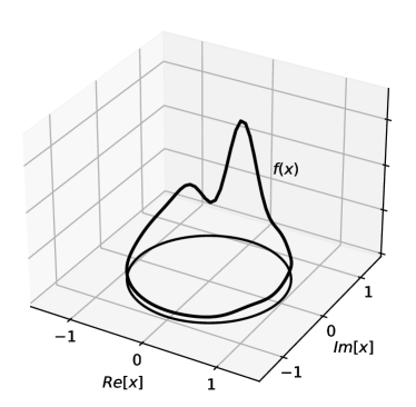
Regarding if-clause, $control_{\phi}(U)=control_{\phi}^{1}(U)$, Araújo, Feix, Costa and Brukner [araujo_cU] proved its impossibility from one query in a quantum circuit, even though one query suffices in an optics experiment (Fig. 1). They explained that the gate $U$ in Fig. 1 is not completely unknown: its position is known, revealing which path-modes of a photon remain unaffected. The gate acts on those $d$ modes as the identity, so that on the $2d$ modes of the two paths it acts as $I_{d}\oplus U=control_{0}(U)$! Araújo et al. argued that $I\oplus U$ correctly describes any physical gate restricted to specific space and time, and the composition via direct sum $\oplus$ should be added to the quantum circuit formalism [araujo_cU]. We have two comments. If already changing the model, instead of this ad hoc modification ($I_{d}\oplus U$ emerges when viewing Fig. 1 in the first quantisation), we suggest switching to a proper model for optics – arising from the second quantisation, such as boson sampling [aaronson2011computational] or holomorphic computation [chabaud2021holomorphic]. But more importantly, is modifying the model really necessary? The impossibility of if-clause from one query is not significant from the complexity point of view. A quantum circuit could still succeed with polynomially many queries. In the absence of oracles, the quantum circuit model can simulate optics with only a polynomial overhead [feynman1982simulating, abrams1997simulation, bravyi2002fermionic, aaronson2011computational]. But if-clause requires oracle queries. We are interested in its query complexity as a function of $n=\lceil\log_{2}d\rceil$, the number of qubits the oracle $U\in U(d)$ acts on. The linear-optics complexity of if-clause is constant, $1$. How much larger is its quantum-circuit complexity? Seemingly at most exponential in $n$. Using Solovay-Kitaev theorem [nielsen2002quantum] we can implement $control_{0}(U)$ from $U$’s classical description, obtained by process tomography [chuang1997prescription, poyatos1997complete, leung2000towards]: by setting an input to the oracle and measuring the output enough times to obtain statistics, repeating for different inputs and measurement settings, then calculating the oracle’s matrix from all the measurement statistics. Process tomography requires $\exp(n)$ queries.

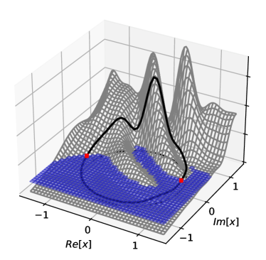
Surprisingly, we show that the quantum-circuit complexity of the quantum if-clause is infinite. Our quantum circuit model is a unitary circuit followed by a binary success/fail measurement and a postselection on the success outcome. No matter how many times such a circuit queries $U$ and $U^{\dagger}$, it cannot implement $control_{\phi}(U)$ for some function $\phi$ with nonzero success probability for every $U\in U(d)$ – not even with a constant precision error! Process tomography, suggested above, fails to estimate the oracle in a useful way: If-clause requires a matrix estimate, instead of a superoperator estimate – we show the limitations of such matrix tomography. To arrive at our results, we develop a new ”lower bound” method. We observe that any quantum circuit corresponds to a continuous function, then we use topology to show that no continuous function can have the desired output. In Table 2 we compare this method to impossibility methods that treat quantum circuits as linear or polynomial functions: Our topological method has a limited applicability but gives the strongest impossibility.

Table 2: Impossibility methods that regard quantum circuits as functions

impossibility method	some applications	number of queries it excludes
linear	cloning [no_cloning], deleting [no_deleting], if-clause [araujo_cU]	1 or a task with no oracle
polynomial [lbounds_polynomials]	boolean functions: their query [aaronson2004collision, sherstov2013andor, bun2015andor, bun2018polynomial, aaronson2020counting] and communication [sherstov2011pattern, sherstov2012multiparty] complexity; oracle separations [beigel1994perceptrons, bouland2019power]	smaller than half the degree of the polynomial
our topological method	operations with quantum input and output: deterministic if-clause*, fractional power*, superposing unknown states [gavorova2021topologically]	any finite number

• this result (for its application to fractional power see LABEL:section_worst-case)

We first made the connection to topology via Borsuk-Ulam theorem (Fig. 2). LABEL:section_bu uses it to prove the if-clause impossibility for even dimensions $d$. For the general case we employ a new topological lemma about $m$-homogeneous functions, which are functions $f$ that obey $f(\lambda x)=\lambda^{m}f(x)$ for any input $x$ and any scalar $\lambda$.

Figure 2: The Borsuk-Ulam theorem states that any continuous function $f:S^{n}\to\mathbb{R}^{n}$ has a pair of opposite points $x,-x$ that map to the same value $f(x)=f(-x)$. Here we give the intuition for the $n=1$ case: At some moment the rising tide must hit points that are exactly opposite on the circle.

Lemma 1.

If there exists a continuous $m$-homogeneous function $f:U(d)\rightarrow S^{1}$, then $m$ is a multiple of $d$.

For example the determinant, computed as part of the $control^{d}_{\phi}$ algorithm [dong_controlled] (LABEL:section_cUd), is a $d$-homogeneous function: $\smash{\det(\lambda U)=\lambda^{d}\det(U)}$. By 1 this homogeneity and its multiples are the only ones possible for continuous functions $U(d)\rightarrow S^{1}$. As a result, we complete the $control^{m}_{\phi}$ question into a dichotomy in the parameter $m$: we show that not only if-clause, but any $control^{m}_{\phi}(U)$ with $m$ not a multiple of $d$ is impossible in a quantum circuit.

Our results expose big differences between various computational models. First, the gap between the quantum-circuit complexity and the linear-optics complexity of the quantum if-clause is infinite. Moreover, the gap does not shrink by removing the requirement of causal order from quantum circuits. We show that our impossibility extends to quantum circuits with relaxed causal order, called process matrices or supermaps [chiribella2013quantum]. Process matrices have attracted a lot of attention since the discovery of the task of superposing the order of two oracles, the quantum switch task [chiribella2013quantum]. While process matrices are believed to better capture the linear-optics implementation of quantum switch [araujo2014computational], on if-clause they fail as badly as the quantum circuit (see LABEL:sec_process_matrix). The last difference appears when analysing matrix tomography for building an if-clause circuit. To succeed on all oracles $U\in U(d)$, the tomography must rely on many-outcome measurements. This brings in randomness in the choice of phase, and, instead of if-clause, implements random if-clause: an operator $control_{\phi_{j}}(U)$ where $j$ is a random index depending on the measurement outcomes. On random if-clause, quantum circuits that use measurements with multiple success outcomes are more powerful than those with one success outcome (Table 1).

Not all hope is lost for the deterministic quantum circuit model. A modification of the matrix-tomography strategy could defer and then skip the measurements, implementing entangled if-clause, in which the relative phase $\phi_{j}$ in each $control_{\phi_{j}}(U)$ is entangled to an additional register encoding $\left|j\right>$. Either way, relaxing the if-clause definition is necessary for any quantum circuit solution.

2 Algorithm as a continuous function

It is instructive to formulate our problem in terms of functions on linear operators. For example $control_{\phi}:U(d)\to L(\mathcal{H})$ is a function that maps unitaries to the space of linear operators from a finite-dimensional Hilbert space $\mathcal{H}$ to itself, denoted $L(\mathcal{H})$. The function accepts an oracle and outputs the linear operator we wish to implement. Such function we call the task function. We allow queries to the oracle $U$ and to its inverse $U^{\dagger}$. We represent these two types of queries by functions on operators as well: $id:U\mapsto U$ and $inv:U\mapsto U^{\dagger}$ respectively. They specify the allowed ways to query the oracle, therefore we call them query functions. Other examples of query functions are $control_{0}$ in phase estimation [kitaev95] or a $d$-th root of $U$ in the algorithm for building $control_{\phi}(U)$ from fractions [dong_controlled]. The collection of the allowed query functions is called the query alphabet. The task function and the query alphabet together form a task – so our task is $(control_{\phi},\{id,inv\})$ for some $\phi$. See Table 3 and LABEL:section_tasks for additional examples.

Table 3: Examples of tasks and their approximate solvability by a postselected circuit

task	formally	possible for all $U\in U(d)$	for most $U\in U(d)$
if-clause	$(control_{\phi},\{id,inv\})$x	✘*	✔ (unitary) [dong_controlled, sheridan_maslov_mosca]y
$\quad\cdot$ from fractions	$(control_{\phi},\{U\mapsto U^{q}\}_{q\in\mathbb{Q}})$x	✔ (exact, unitary) [dong_controlled]
complex conjugate	$(U\mapsto U^{*},\{id\})$	✔ (exact, unitary) [compl_conj]
transpose	$(U\mapsto U^{T},\{id\})$	✔ (exact) [quintino_transforming, quintino_inverse]
inverse	$(inv,\{id\})$	✔ (exact) [quintino_transforming, quintino_inverse, compl_conj]y
phase estimation	$(phase\_est,\{id,control_{0}\})$	✔ (unitary) [kitaev95]
fractional power	$(U\mapsto U^{q},\{id,inv\}),q\in\mathbb{Q}$	✘ [dong_controlled]*y	✔ (unitary) [sheridan_maslov_mosca]

• this result (for its application to the fractional power see LABEL:section_worst-case)

• $control_{\phi}:U\mapsto\left|0\right>\!\!\left<0\right|\otimes I+e^{i\phi(U)}\left|1\right>\!\!\left<1\right|\otimes U$, where $\phi$ is any real function

• by composing two tasks

We also formulate an algorithm as a function on operators: The input is the oracle and the output is the linear operator implemented by the algorithm to all its Hilbert spaces, ancillae included. Therefore, an algorithm is a function $A:U(d)\mapsto L(\mathcal{H}\otimes\mathcal{K})$, where $\mathcal{K}$ is the ancilla Hilbert space. See Fig. 3(a) for a general algorithm that corresponds to the quantum circuit model with a binary measurement $\{\Pi_{\text{succ}},\Pi_{\text{fail}}\}$ and a postselection on success. Fig. 3(a) can equivalently be expressed by the operator equation

$$A(U)=\Pi_{\text{succ}}V_{N}\left(\sigma_{N}(U)\otimes I_{\mathcal{K}_{N}}\right)\dots V_{1}\left(\sigma_{1}(U)\otimes I_{\mathcal{K}_{1}}\right)V_{0}$$ (3)

We impose the usual postselection condition that the probability of success is nonzero

$$p_{\text{succ}}(U,\left|\xi\right>)=\left|\left|A(U)\left(\left|\xi\right>\otimes\left|\mathbf{0}\right>\right)\right|\right|^{2}>0$$ (4)

for all oracles $U\in U(d)$ and all inputs $\left|\xi\right>\in\mathcal{H}$ (the ancillae are initialised to the all-zero state). We call an algorithm that satisfies eqs. 3 and 4 a postselection oracle algorithm.

We say that a postselection oracle algorithm $A$ exactly achieves the task $(t,\Sigma)$ if it: 1) makes queries from the task’s query alphabet $\sigma_{i}\in\Sigma$ and 2) implements $t(U)$ to the Hilbert space $\mathcal{H}$, provided that the ancilla Hilbert space $\mathcal{K}$ was properly initialised. We express this formally by the operator equation

$$A(U)\left(I_{\mathcal{H}}\otimes\left|\mathbf{0}\right>\!\!\left<\boldsymbol{0}\right|\right)=t(U)\otimes\left|g(U)\right>\!\!\left<\boldsymbol{0}\right|$$ (5)

for some $\left|g(U)\right>\in\mathcal{K}$. In LABEL:section_cUno_approx we replace the equality by an inequality to define $\epsilon$-approximately achieving. The inequality is such that for a unitary algorithm ($\Pi_{\text{succ}}=I$) $\epsilon$ measures the trace-induced distance of the superoperators corresponding to the algorithm and the task. For an algorithm that includes postselection ($\Pi_{\text{succ}}\neq I$) we use the trace-induced distance for the postselected setting [technical]. While diamond distance is more physical, using its lower bound, the trace-induced distance, makes our result stronger. By Theorem 1 (next section) all algorithms must have large trace-induced distance from the task (large $\epsilon$). It follows that the diamond distance is at least as large.

We formulated an algorithm as a function on operators to be able to discuss two properties: continuity and homogeneity. By eq. 3 a postselection oracle algorithm inherits the continuity and homogeneity from its query alphabet: If all query functions $\sigma_{i}$ are continuous, then so is $A$; if all query functions are homogeneous, $\sigma_{i}(\lambda U)=\lambda^{m_{i}}\sigma_{i}(U)$, then so is the algorithm, $A(\lambda U)=\lambda^{\sum_{i=1}^{N}m_{i}}A(U)$.

3 The Dichotomy Theorem

$$\leavevmode\hbox to341.21pt{\vbox to63.85pt{\pgfpicture\makeatletter\hbox{\hskip-20.73958pt\lower-34.74321pt\hbox to0.0pt{\pgfsys@beginscope\pgfsys@invoke{ }\definecolor{pgfstrokecolor}{rgb}{0,0,0}\pgfsys@color@rgb@stroke{0}{0}{0}\pgfsys@invoke{ }\pgfsys@color@rgb@fill{0}{0}{0}\pgfsys@invoke{ }\pgfsys@setlinewidth{0.4pt}\pgfsys@invoke{ }\nullfont\hbox to0.0pt{\pgfsys@beginscope\pgfsys@invoke{ } {}{{}}{} {{}{}}{{}}{}{}{}{}{{}}{}\pgfsys@beginscope\pgfsys@invoke{ }\definecolor{pgfstrokecolor}{rgb}{0.295,0.295,0.295}\pgfsys@color@gray@stroke{0.295}\pgfsys@invoke{ }\pgfsys@setlinewidth{1.2pt}\pgfsys@invoke{ }\pgfsys@setdash{3.0pt,3.0pt}{0.0pt}\pgfsys@invoke{ }{}\pgfsys@moveto{21.33957pt}{-34.14322pt}\pgfsys@moveto{21.33957pt}{-34.14322pt}\pgfsys@lineto{21.33957pt}{14.22638pt}\pgfsys@lineto{361.34995pt}{14.22638pt}\pgfsys@lineto{361.34995pt}{-34.14322pt}\pgfsys@closepath\pgfsys@moveto{361.34995pt}{14.22638pt}\pgfsys@stroke\pgfsys@invoke{ } \pgfsys@invoke{\lxSVG@closescope }\pgfsys@endscope{{}}\hbox{\hbox{{\pgfsys@beginscope\pgfsys@invoke{ }{{}{}{{ {}{}}}{ {}{}} {{}{{}}}{{}{}}{}{{}{}} { }{{{{}}\pgfsys@beginscope\pgfsys@invoke{ }\pgfsys@transformcm{1.0}{0.0}{0.0}{1.0}{206.0655pt}{18.27039pt}\pgfsys@invoke{ }\hbox{{\definecolor{.}{rgb}{0.295,0.295,0.295}\definecolor[named]{pgfstrokecolor}{rgb}{0.295,0.295,0.295}\pgfsys@color@gray@stroke{0.295}\pgfsys@invoke{ }\pgfsys@color@gray@fill{0.295}\pgfsys@invoke{ }\hbox{{\definecolor{.}{rgb}{0.295,0.295,0.295}\color[rgb]{0.295,0.295,0.295}\definecolor[named]{pgfstrokecolor}{rgb}{0.295,0.295,0.295}\pgfsys@color@gray@stroke{0.295}\pgfsys@color@gray@fill{0.295}$\boldsymbol{A(U)}$}} }}\pgfsys@invoke{\lxSVG@closescope }\pgfsys@endscope}}} \pgfsys@invoke{\lxSVG@closescope }\pgfsys@endscope}}} \pgfsys@invoke{\lxSVG@closescope }\pgfsys@endscope{}{}{}\hss}\pgfsys@discardpath\pgfsys@invoke{\lxSVG@closescope }\pgfsys@endscope\hss}}\lxSVG@closescope\endpgfpicture}}\Qcircuit@C=1em@R=.3em{&\push{{}_{\mathcal{H}}}\qw\multigate{2}{V_{0}}\gate{\sigma_{1}(U)}\multigate{2}{V_{1}}\gate{\sigma_{2}(U)}\multigate{2}{V_{2}}\qw\gate{\sigma_{N}(U)}\multigate{2}{V_{N}}\multigate{2}{\Pi_{\text{succ}}}\push{{}_{\mathcal{H}}}\qw\qw\\ \pureghost{V_{0}}\pureghost{V_{1}}\pureghost{V_{2}}\push{\dots}\pureghost{V_{N}}\pureghost{\Pi_{\text{succ}}}\\ \lstick{\left|\boldsymbol{0}\right>}\push{{}_{\mathcal{K}}}\qw\ghost{V_{0}}\push{{}_{\mathcal{K}_{1}}}\qw\ghost{V_{1}}\push{{}_{\mathcal{K}_{2}}}\qw\ghost{V_{2}}\qw\push{{}_{\mathcal{K}_{N}}}\qw\ghost{V_{N}}\ghost{\Pi_{\text{succ}}}\push{{}_{\mathcal{K}}}\qw\qw} \boldsymbol{A(U)} \boldsymbol{A(U)}$$

(a)

$$\leavevmode\hbox to244.69pt{\vbox to71.53pt{\pgfpicture\makeatletter\hbox{\hskip 46.9167pt\lower-43.27913pt\hbox to0.0pt{\pgfsys@beginscope\pgfsys@invoke{ }\definecolor{pgfstrokecolor}{rgb}{0,0,0}\pgfsys@color@rgb@stroke{0}{0}{0}\pgfsys@invoke{ }\pgfsys@color@rgb@fill{0}{0}{0}\pgfsys@invoke{ }\pgfsys@setlinewidth{0.4pt}\pgfsys@invoke{ }\nullfont\hbox to0.0pt{\pgfsys@beginscope\pgfsys@invoke{ } {}{{}}{} {{}{}}{{}}{}{}{}{}{{}}{}\pgfsys@beginscope\pgfsys@invoke{ }\definecolor{pgfstrokecolor}{rgb}{0.0546875,0.11796875,0.38359375}\pgfsys@color@rgb@stroke{0.0546875}{0.11796875}{0.38359375}\pgfsys@invoke{ }\pgfsys@setlinewidth{1.2pt}\pgfsys@invoke{ }\pgfsys@setdash{3.0pt,3.0pt}{0.0pt}\pgfsys@invoke{ }{}\pgfsys@moveto{5.69046pt}{-42.67914pt}\pgfsys@moveto{5.69046pt}{-42.67914pt}\pgfsys@lineto{5.69046pt}{12.80365pt}\pgfsys@lineto{197.1774pt}{12.80365pt}\pgfsys@lineto{197.1774pt}{-42.67914pt}\pgfsys@closepath\pgfsys@moveto{197.1774pt}{12.80365pt}\pgfsys@stroke\pgfsys@invoke{ } \pgfsys@invoke{\lxSVG@closescope }\pgfsys@endscope{{}}\hbox{\hbox{{\pgfsys@beginscope\pgfsys@invoke{ }{{}{}{{ {}{}}}{ {}{}} {{}{{}}}{{}{}}{}{{}{}} { }{{{{}}\pgfsys@beginscope\pgfsys@invoke{ }\pgfsys@transformcm{1.0}{0.0}{0.0}{1.0}{67.88864pt}{17.41684pt}\pgfsys@invoke{ }\hbox{{\definecolor{.}{rgb}{0.0546875,0.11796875,0.38359375}\definecolor[named]{pgfstrokecolor}{rgb}{0.0546875,0.11796875,0.38359375}\pgfsys@color@rgb@stroke{0.0546875}{0.11796875}{0.38359375}\pgfsys@invoke{ }\pgfsys@color@rgb@fill{0.0546875}{0.11796875}{0.38359375}\pgfsys@invoke{ }\hbox{{\definecolor{.}{rgb}{0.0546875,0.11796875,0.38359375}\color[rgb]{0.0546875,0.11796875,0.38359375}\definecolor[named]{pgfstrokecolor}{rgb}{0.0546875,0.11796875,0.38359375}$\boldsymbol{C(U)}$}} }}\pgfsys@invoke{\lxSVG@closescope }\pgfsys@endscope}}} \pgfsys@invoke{\lxSVG@closescope }\pgfsys@endscope}}} \pgfsys@beginscope\pgfsys@invoke{ }{{}} {{}}\hbox{\hbox{{\pgfsys@beginscope\pgfsys@invoke{ }{{}{}{{ {}{}}}{ {}{}} {{}{{}}}{{}{}}{}{{}{}} { }{{{{}}\pgfsys@beginscope\pgfsys@invoke{ }\pgfsys@transformcm{1.0}{0.0}{0.0}{1.0}{-43.5837pt}{-8.25359pt}\pgfsys@invoke{ }\hbox{{\definecolor{pgfstrokecolor}{rgb}{0,0,0}\pgfsys@color@rgb@stroke{0}{0}{0}\pgfsys@invoke{ }\pgfsys@color@rgb@fill{0}{0}{0}\pgfsys@invoke{ }\hbox{{$\mathcal{H}$}} }}\pgfsys@invoke{\lxSVG@closescope }\pgfsys@endscope}}} \pgfsys@invoke{\lxSVG@closescope }\pgfsys@endscope}}} {}{{}}{} {}{} {}{{}{}}{}{}{}{{}}{{}}{{}{}}{{}{}}{{{{}{}{{}} }}{{}} {} {}{}{} { {{}} {} {}{}{} {}{}{} } { {{}} {} {}{}{} } }{{}{}}{{}{}}{{{{}{}{{}} }}{{}}} {}\pgfsys@moveto{-25.60732pt}{-20.48602pt}\pgfsys@moveto{-25.60732pt}{-20.48602pt}\pgfsys@curveto{-27.31448pt}{-19.63248pt}{-28.45259pt}{-17.64075pt}{-28.45259pt}{-14.79547pt}\pgfsys@lineto{-28.45259pt}{-10.52748pt}\pgfsys@curveto{-28.45259pt}{-7.6822pt}{-29.59068pt}{-5.69048pt}{-31.29787pt}{-4.83693pt}\pgfsys@curveto{-29.59068pt}{-3.98338pt}{-28.45259pt}{-1.99165pt}{-28.45259pt}{0.85362pt}\pgfsys@lineto{-28.45259pt}{5.12161pt}\pgfsys@curveto{-28.45259pt}{7.96689pt}{-27.31448pt}{9.95862pt}{-25.60732pt}{10.81216pt}\pgfsys@stroke\pgfsys@invoke{ } \pgfsys@invoke{\lxSVG@closescope }\pgfsys@endscope \pgfsys@invoke{\lxSVG@closescope }\pgfsys@endscope{}{}{}\hss}\pgfsys@discardpath\pgfsys@invoke{\lxSVG@closescope }\pgfsys@endscope\hss}}\lxSVG@closescope\endpgfpicture}}\Qcircuit@C=1em@R=.3em{\lstick{\left|0\right>_{\phantom{\mathcal{K}}}}&\multigate{2}{{\color[rgb]{0.295,0.295,0.295}\definecolor[named]{pgfstrokecolor}{rgb}{0.295,0.295,0.295}\pgfsys@color@gray@stroke{0.295}\pgfsys@color@gray@fill{0.295}\boldsymbol{A(U)}}}\gate{X}\multigate{2}{{\color[rgb]{0.295,0.295,0.295}\definecolor[named]{pgfstrokecolor}{rgb}{0.295,0.295,0.295}\pgfsys@color@gray@stroke{0.295}\pgfsys@color@gray@fill{0.295}\boldsymbol{A(U)^{\dagger}}}}\qw\gate{X}\qw\\ \lstick{\left|0\right>_{\phantom{\mathcal{K}}}}\ghost{\boldsymbol{A(U)}}\qw\ghost{\boldsymbol{A(U)}^{\dagger}}\qw\gate{U^{m}}\qw\\ \lstick{\left|\boldsymbol{0}\right>_{\mathcal{K}}}\ghost{\boldsymbol{A(U)}}\qw\ghost{\boldsymbol{A(U)}^{\dagger}}\gate{\left|\boldsymbol{0}\right>\!\!\left<\boldsymbol{0}\right|_{\mathcal{K}}}\qw\qw} \boldsymbol{C(U)} \mathcal{H} \boldsymbol{C(U)} \mathcal{H}$$

(b)

(c)

Figure 3: (a) A general postselection oracle algorithm $A:U(d)\to L(\mathcal{H}\otimes\mathcal{K})$: It has fixed unitary gates $V_{0}\dots V_{N}$, a fixed projection $\Pi_{\text{succ}}$ and $N$ special slots for queries to the oracle $U\in U(d)$. For each slot the type of the query is specified by the query function $\sigma_{i}$. The slot’s Hilbert space $\mathcal{H}_{i}$ matches the query function $\sigma_{i}:U(d)\to L(\mathcal{H}_{i})$ and the identity is applied to the remaining Hilbert space $\mathcal{K}_{i}$. (b) Towards proving that $A$ cannot exist we build from it a new algorithm $C$. $C(U)$ also acts on $\mathcal{H}\otimes\mathcal{K}$, but the control qubit and the target qudit that constitute $\mathcal{H}$ are shown explicitly. The circuit also contains Pauli-$X$ flips of the control and a projection of the ancilla ($\mathcal{K}$) register onto the all-zero state. (c) Sequential and simultaneous increase of each coordinate are homotopic inside the cube $[0,1]^{3}$.

Here we show that implementing the quantum if-clause, or $control_{\phi}(U)$ for all $U\in U(d)$, is impossible. Our result is actually more general, concerned with $control^{m}_{\phi}$ for integer powers $m\in\mathbb{Z}$. We show the following dichotomy:

Theorem 1.

Let ${m}\in\mathbb{Z}$. Let $d\in\mathbb{N}$ and consider oracles of this dimension, $U\in U(d)$. Let $\epsilon\in\left[0,\tfrac{1}{2}\right)$.

• If $d|m$ there exists a postselection oracle algorithm $\epsilon$-approximately achieving the task

  $$\text{c-}U^{m}=(U\mapsto\left|0\right>\!\!\left<0\right|\otimes I+e^{i\phi(U)}\left|1\right>\!\!\left<1\right|\otimes U^{m},\{id,inv\})\text{,}$$

  for some $\phi:U(d)\to\mathbb{R}$.

• If $d\nmid m$ no such postselection oracle algorithm exists.

The quantum if-clause is the special case when $m=1$. Its impossibility follows as any nontrivial dimension $d\geq 2$ of the oracle does not divide $m=1$.

Proof of the exact case.

The $d|m$ direction of the theorem follows from the exact algorithm of Dong and others [dong_controlled] (reviewed in LABEL:section_cUd). The algorithm exactly implements $control_{\phi}^{d}(U)$ from $id$ queries (or equivalently $control_{\phi}(U)$ assuming queries to $d$-th roots $\smash{U\mapsto U^{\frac{1}{d}}}$ – listed as ”if-clause from fractions” in Table 3). To implement $control_{\phi}^{m}(U)$ one only needs to repeat this algorithm $\left|\tfrac{m}{d}\right|$ times and switch the $id$ queries to $inv$ queries if $m$ is negative.

Our main contribution is the impossibility for the case when $d\nmid m$. Here we prove it for $\epsilon=0$. First, we assume the existence of a postselection oracle algorithm $A$ that exactly achieves the task c-$U^{m}$, then, we build from $A$ a function of 1. Since $A$ exactly achieves a task with query alphabet $\{id,inv\}$ that contains only continuous functions, $A$ must be continuous. Since $id$ is $1$-homogeneous and $inv$ is $(-1)$-homogeneous, $A$ is $w$-homogeneous for some $w\in\mathbb{Z}$ (equal to the algorithm’s number of $id$ queries minus the number of $inv$ queries). By eq. 5 we have

$$A(U)\left(I_{\mathcal{H}}\otimes\left|\mathbf{0}\right>\!\!\left<\boldsymbol{0}\right|_{\mathcal{K}}\right)=\left(\left|0\right>\!\!\left<0\right|\otimes I+e^{i\phi(U)}\left|1\right>\!\!\left<1\right|\otimes U^{m}\right)\otimes\left|g(U)\right>\!\!\left<\boldsymbol{0}\right|_{\mathcal{K}}\text{.}$$

Next, we build the circuit of Fig. 3(b). The output of this circuit is $C(U)\left|\mathbf{0}\right>=e^{-i\phi(U)}\left|\left|\,\left|g(U)\right>\right|\right|^{2}\left|\mathbf{0}\right>$, where $\left|\mathbf{0}\right>\in\mathcal{H}\otimes\mathcal{K}$ is the all-zero state on all registers. Moreover, $C:U(d)\to L(\mathcal{H}\otimes\mathcal{K})$ is continuous and $m$-homogeneous. The function

$$f(U):=\frac{\left<\boldsymbol{0}\right|C(U)\left|\mathbf{0}\right>}{\left<\boldsymbol{0}\right|A(U)^{\dagger}A(U)\left|\mathbf{0}\right>}$$

is then continuous, $m$-homogeneous and well-defined: By eq. 4 the denominator $\left|\left|A(U)\left|\mathbf{0}\right>\right|\right|^{2}=\left|\left|\,\left|g(U)\right>\right|\right|^{2}=p_{\text{succ}}(U,\left|\mathbf{0}\right>_{\mathcal{H}})$ is never zero. Observe that $f(U)=e^{-i\phi(U)}$. 1 applies to $f$ and concludes that $d|m$, completing the $\epsilon=0$ proof.

In LABEL:section_cUno_approx we prove Theorem 1 for any $\epsilon<\frac{1}{2}$ by building a function of 1 from any algorithm that $\epsilon$-approximately achieves c-$U^{m}$. For intuition, observe that if $A$ has errors, then $\left<\boldsymbol{0}\right|C(U)\left|\mathbf{0}\right>$ are points on a distorted circle in the complex plane. If the distortions are small enough to never hit zero, the distorted circle remains topologically equivalent to $S^{1}$ and 1 still applies.

4 Proof of the topological lemma

Our proof of 1 exploits the structure of the space of unitaries $U(d)$. Specifically, the elementary proof that follows (for a shorter proof see LABEL:section_top_short) finds paths on this space that are continuously deformable, or homotopic, to each other. Formally, let $p(t)$, $p^{\prime}(t)$ be two paths on some space $X$, parametrised by $t\in[0,1]$, with a common start $p(0)=p^{\prime}(0)$ and end $p(1)=p^{\prime}(1)$. The paths $p,p^{\prime}$ are homotopic, if there exists a continuous deformation, corresponding to a continuous function $h(t,s)\in X$ that uses the additional parameter $s\in[0,1]$ to ’deform’ $p(t)=h(t,0)$ into $p^{\prime}(t)=h(t,1)$, while fixing the start and the end, $h(0,s)=p(0)$, $h(1,s)=p(1)$. As an example, Fig. 3(c) illustrates a ’straight line’ homotopy $h(t,s)=(1-s)p(t)+sp^{\prime}(t)$ inside a cube $X=[0,1]^{3}$ between the path $p$ along the cube’s body diagonal and $p^{\prime}$ along its edges.

On our space of unitaries $X=U(d)$, we will denote a path by $U(t)$, $t\in[0,1]$. We split $[0,1]$ to $d$ identical intervals labeled by $j\in\{0,1\dots,d-1\}$ and use the parameter $\Delta\in[0,1]$ to move inside each interval. Consider the paths