Could PBHs and secondary GWs have originated from squeezed initial states?

Abstract

Recently, the production of primordial black holes (PBHs) and secondary gravitational waves (GWs) due to enhanced scalar power on small scales have garnered considerable attention in the literature. Often, the mechanism considered to arrive at such increased power involves a modification of the standard slow roll inflationary dynamics, achieved with the aid of fine-tuned potentials. In this work, we investigate another well known method to generate features in the power spectrum wherein the initial state of the perturbations is assumed to be squeezed states. The approach allows one to generate features even in slow roll inflation with a specific choice for the Bogoliubov coefficients characterizing the squeezed initial states. Also, the method is technically straightforward to implement since the Bogoliubov coefficients can be immediately determined from the form of the desired spectrum with increased scalar power at small scales. It is known that, for squeezed initial states, the scalar bispectrum is strongly scale dependent and the consistency condition governing the scalar bispectrum in the squeezed limit is violated. In fact, the non-Gaussianity parameter $f_{{}_{\rm NL}}$ characterizing the scalar bispectrum proves to be inversely proportional to the squeezed mode and this dependence enhances its amplitude at large wave numbers making it highly sensitive to even a small deviation from the standard Bunch-Davies vacuum. These aspects can possibly aid in leading to enhanced formation of PBHs and generation of secondary GWs. However, we find that: (i) the desired form of the squeezed initial states may be challenging to achieve from a dynamical mechanism, and (ii) the backreaction due to the excited states severely limits the extent of deviation from the Bunch-Davies vacuum at large wave numbers. We argue that, unless the issue of backreaction is circumvented, squeezed initial states cannot lead to a substantial increase in power on small scales that is required for enhanced formation of PBHs and generation of secondary GWs.

1 Introduction

It is now almost half-a-century since it was originally argued that black holes could have formed due to over-densities in the primordial universe [1, 2]. The investigations of such primordial black holes (PBHs) have gained traction over the last few years with the observations of gravitational waves (GWs) from the mergers of binary black holes [3, 4, 5, 6]. Several current and upcoming observational efforts promise to provide constraints on the fraction of the PBHs constituting the bulk of cold dark matter density in the current universe, a quantity usually referred to as $f_{{}_{\mathrm{PBH}}}$ [7]. Motivated by these observational efforts, there has been several attempts to build models of inflation that could generate considerable population of PBHs over certain mass ranges (see, for example, refs. [8, 9, 10, 11, 12]).

It is well known that scales smaller than those associated with the cosmic microwave background (CMB), say, with wave numbers $k>1\,{\mathrm{Mpc}}^{-1}$, reenter the Hubble radius during the radiation dominated epoch. If the scalar power over these small scales have enhanced amplitudes (when compared to their COBE normalized values over the CMB scales), they could, in principle, induce instantaneous collapses of energy densities of corresponding sizes, thereby forming PBHs [13, 14, 15]. To achieve a higher amplitude in the inflationary scalar perturbation spectrum (say, of the order of $10^{-2}$) at larger wave numbers, one has to suitably model the background dynamics so that a departure from slow roll inflation arises at late times. It has been found that, in single field models, inflationary potentials containing a point of inflection can generate the required boost in the scalar power (see, for instance, refs. [11, 16, 17, 18]). The inflection point in the potential leads to a transient epoch of ultra slow roll inflation, which turns out to be responsible for the rise in the scalar power over small scales. Other features, such as a bump or dip artificially added to the potential are also known to boost the scalar power at larger wave numbers [19, 20]. There have also been attempts to generate PBHs using other mechanisms such as models involving non-canonical scalar fields [21, 22], inflation driven by multiple fields [23, 24, 25, 26, 27], inducing a non-trivial speed of sound during inflation [28, 29, 30], or a modified history of reheating and radiation dominated era following inflation [31, 32].

Moreover, when the scalar power is boosted to large amplitudes, the second order tensor perturbations that are sourced by the quadratic terms involving the first order scalar perturbations can dominate the contributions due to the original, inflationary, first order tensor perturbations [33, 34]. In other words, the enhanced scalar power, apart from producing a significant amount of PBHs, also leads to considerable amplification of the secondary GWs at small scales or, equivalently, at large frequencies [35]. These GWs induced by the scalar perturbations are expected to be stochastic and isotropic. There are several experiments and observational surveys that constrain the dimensionless energy density of such a stochastic gravitational wave background, say, $\Omega_{{}_{\mathrm{GW}}}$, observable today [36].

As we mentioned above, the enhancement in the scalar power over small scales can be achieved with the aid of a brief period of departure from slow roll inflation. We should point out here that such scenarios would also produce a strongly scale dependent bispectrum. However, it has been shown that, in single field models of inflation wherein the deviation from slow roll is brief, the consistency condition relating the bispectrum and the power spectrum in the squeezed limit is indeed satisfied (in this context, see refs. [37, 17, 38]). This implies that the magnitude of the scalar non-Gaussianity parameter, $f_{{}_{\rm NL}}$, is at the most of order unity over the range of wave numbers which contains enhanced power. As a result, any corrections due to the bispectrum that has to be accounted for in the power spectrum proves to be negligible in these models [17].

However, the aforementioned methods of modifying slow roll inflation to achieve sufficient enhancement in the scalar power, and hence produce significant amount of PBHs and secondary GWs, are known to pose certain challenges. They typically require extreme fine-tuning of the parameters involved. Else, they may either prolong the duration of inflation beyond reasonable number of e-folds or alter the scalar spectral index $n_{{}_{\mathrm{S}}}$ and the tensor-to-scalar ratio $r$ over the CMB scales thereby leading to a tension with the constraints from Planck data (see, for instance, refs. [11, 17]). There exists another approach to achieve power spectra with the desired shape at small scales. The alternative method is to work with non-vacuum, specifically, squeezed, initial states for the perturbations during inflation. This method of evolving the perturbations with initial states other than the standard Bunch-Davies vacuum is well known in the literature and has been discussed in various contexts (see, for example, refs. [39, 40, 41, 42, 43, 44, 45, 46, 47, 48, 49, 50, 51]). These excited initial states for the perturbations can be expressed in terms of the so-called Bogoliubov coefficients. As we shall see, the Bogoliubov coefficients essentially provide us an independent function to introduce the desired features in the power spectrum. However, while it is technically straightforward to arrive at the required power spectrum with a suitable choice of the Bogoliubov coefficients, we encounter two drawbacks with the proposed approach. On the one hand, it seems challenging to design a mechanism that leaves the curvature perturbations in such an excited initial state. On the other hand, we find that squeezed initial states lead to significant backreaction during the early stages of inflation unless the state is remarkably close to the Bunch-Davies vacuum.

To illustrate these points, in this work, we shall focus on the popular lognormal shape of amplification in the scalar power spectrum [35, 52]. In the following section, we shall briefly describe the modes corresponding to squeezed initial states and discuss the corresponding scalar power and bispectra. We shall consider suitable functional forms for the Bogoliubov coefficients to produce the lognormal feature in the power spectrum and calculate the corresponding scalar bispectrum analytically. We shall show that the bispectrum is significantly enhanced in the squeezed limit and that the consistency condition is strongly violated over the range of wave numbers containing the lognormal feature. In other words, we find that the cubic order non-Gaussian modifications to the scalar power spectrum can possibly dominate the amplitude of the original scalar power around the feature for certain values of the parameter that characterizes the deviations from the Bunch-Davies vacuum. In section 3, we shall compute the observable quantities of interest, viz. $f_{{}_{\mathrm{PBH}}}$ and $\Omega_{{}_{\mathrm{GW}}}$, generated from such an enhanced scalar power spectrum. In section 4, we shall first discuss possible mechanisms that can lead to the squeezed initial states for the curvature perturbation at early times. Thereafter, we shall describe the issue of backreaction wherein we compute the energy density associated with the perturbations evolved from squeezed initial states and compare it against the background energy density. We argue that it is rather challenging to achieve such specific initial states by invoking mechanisms operating prior to inflation. Moreover, we find that the backreaction severely restricts the extent of deviation of the initial state from the Bunch-Davies vacuum, particularly on small scales. This, in turn, implies that the desired amplification in the power spectrum and the larger levels of non-Gaussianities cannot be achieved in this approach unless the choice of the specific initial state is satisfactorily justified and the issue of backreaction is overcome. We shall finally conclude in section 5 with a brief summary and outlook.

Before we proceed, we should clarify the conventions and notations that we shall adopt in this work. We shall work with natural units such that $\hbar=c=1$ and set the reduced Planck mass to be $M_{{}_{\mathrm{Pl}}}=\left(8\,\pi\,G\right)^{-1/2}$. We shall assume the background to be the spatially flat Friedmann-Lemaître-Robertson-Walker (FLRW) line element described by the scale factor $a$ and the Hubble parameter $H$. Note that $\eta$ shall represent the conformal time coordinate and an overprime shall denote differentiation with respect to $\eta$.

2 Squeezed initial states, scalar power and bispectra

In this section, we shall construct scalar power spectra with a lognormal peak from squeezed initial states. We shall also calculate the associated scalar bispectra and utilize the result to arrive at the corresponding non-Gaussian modifications to the power spectrum.

As far as the background dynamics is concerned, we shall have in mind the scenario of slow roll inflation. Recall that, in such a case, while it is the combination of the nearly constant Hubble parameter $H_{{}_{\mathrm{I}}}$ and the first slow parameter $\epsilon_{1}$ that determine the amplitude of the scalar power spectrum, the first two slow roll parameters $\epsilon_{1}$ and $\epsilon_{2}$ determine the scalar spectral index $n_{{}_{\mathrm{S}}}$. Moreover, the tensor-to-scalar ratio $r$ is determined by the first slow roll parameter $\epsilon_{1}$. The values of these parameters can be chosen so that we achieve nearly scale invariant scalar and tensor power spectra that are consistent with the recent constraints from Planck over the CMB scales [53]. However, for convenience, in our calculations below, we shall work with the de Sitter modes to describe the scalar perturbations. The modes, say, $f_{k}(\eta)$, describing the scalar perturbations that emerge from initial conditions corresponding to squeezed states can be expressed as [39, 40, 41, 42, 43, 44, 45, 46, 47, 48, 49, 51]

$$f_{k}(\eta)=\frac{i\,H_{{}_{\mathrm{I}}}}{2\,M_{{}_{\mathrm{Pl}}}\,\sqrt{k^{3}\,\epsilon_{1}}}\,\left[\alpha(k)\,\left(1+i\,k\,\eta\right)\,\mathrm{e}^{-i\,k\,\eta}-\beta(k)\,\left(1-i\,k\,\eta\right)\,\mathrm{e}^{i\,k\,\eta}\right],$$ (2.1)

where $\alpha(k)$ and $\beta(k)$ are the so-called Bogoliubov coefficients. Note that the standard Bunch-Davies initial conditions correspond to setting $\alpha(k)=1$ and $\beta(k)=0$. The above modes correspond to squeezed initial states that are excited states above the Bunch-Davies vacuum. We should also mention that the Bogoliubov coefficients $\alpha(k)$ and $\beta(k)$ are not completely independent functions, but satisfy the following constraint:

$$|\alpha(k)|^{2}-|\beta(k)|^{2}=1.$$ (2.2)

This constraint arises due to the fact that the Wronskian associated with the differential equation governing the scalar perturbations is a constant, which is determined by the initial conditions imposed on the modes.

2.1 Power spectrum from squeezed initial states

The power spectrum of the scalar perturbations evolving from squeezed initial states can be evaluated towards the end of inflation (i.e. as $\eta\to 0$). Upon using the modes (2.1), the resulting power spectrum can be expressed in terms of the Bogoliubov coefficients $\alpha(k)$ and $\beta(k)$ as follows:

$${\mathcal{P}}_{{}_{\mathrm{S}}}(k)=\frac{k^{3}}{2\,\pi^{2}}\,|f_{k}(\eta\to 0)|^{2}={\mathcal{P}}_{{}_{\mathrm{S}}}^{0}(k)\,|\alpha(k)-\beta(k)|^{2},$$ (2.3)

where

$${\mathcal{P}}_{{}_{\mathrm{S}}}^{0}(k)=\frac{H_{{}_{\mathrm{I}}}^{2}}{8\,\pi^{2}\,M_{{}_{\mathrm{Pl}}}^{2}\,\epsilon_{1}}$$ (2.4)

is the COBE normalized, nearly scale invariant spectrum with a small red tilt. Since we are interested in the small scale features of the spectrum, for simplicity, we shall assume that ${\mathcal{P}}_{{}_{\mathrm{S}}}^{0}(k)$ is strictly scale invariant with a COBE normalized amplitude over all the wave numbers of our interest. We should hasten to add that introducing a small red tilt does not affect our conclusions in the remainder of our discussion. We shall choose to work with the following values of the primary slow roll inflationary parameters: $H_{{}_{\mathrm{I}}}=4.16\times 10^{-5}\,M_{{}_{\mathrm{Pl}}}$, $\epsilon_{1}=10^{-2}$ and $\epsilon_{2}=2\,\epsilon_{1}$. Also, note that the power spectrum is independent of an overall phase factor and depends only on the relative phase factor between $\alpha(k)$ and $\beta(k)$.

Let us now define $\delta(k)=\beta(k)/\alpha(k)$. Then, upon using the constraint (2.2), the power spectrum (2.3) can be written in terms of the function $\delta(k)$ as

$${\mathcal{P}}_{{}_{\mathrm{S}}}(k)={\mathcal{P}}_{{}_{\mathrm{S}}}^{0}(k)\,\left[\frac{|1-\delta(k)|^{2}}{1-|\delta(k)|^{2}}\right].$$ (2.5)

For ease of modeling, we shall assume the relative phase factor between $\alpha(k)$ and $\beta(k)$ to be zero. We should clarify that this assumption is made just to simplify our calculations. It can be relaxed, if needed, to model the spectrum with the phase factor taken into account. Setting the relative phase factor to be zero essentially implies that $\delta(k)$ is real so that the above expression for the scalar power spectrum reduces to

$${\mathcal{P}}_{{}_{\mathrm{S}}}(k)={\mathcal{P}}_{{}_{\mathrm{S}}}^{0}(k)\,\left\{\frac{\left[1-\delta(k)\right]^{2}}{1-\delta^{2}(k)}\right\}.$$ (2.6)

With the above form of the spectrum arising from squeezed initial states, we shall now proceed to model the feature of our interest. Let us assume that the power spectrum has a localized feature over a certain range of wave numbers, say, $g(k)$, so that ${\mathcal{P}}_{{}_{\mathrm{S}}}(k)$ is given by

$${\mathcal{P}}_{{}_{\mathrm{S}}}(k)={\mathcal{P}}_{{}_{\mathrm{S}}}^{0}(k)\,\left[1+g(k)\right].$$ (2.7)

Upon comparing the above two equations, it is evident that the feature $g(k)$ is related to $\delta(k)$ as follows:

$$\delta(k)=\,\frac{-g(k)}{2+g(k)}$$ (2.8)

It should be clear that we have essentially traded off the function $g(k)$ for $\delta(k)$. In other words, we can choose an initial squeezed state described by $\delta(k)$ to lead to the desired feature $g(k)$ in the power spectrum. In this work, we shall assume $g(k)$ to be a lognormal function of the wave number $k$. Such a form for the feature in the spectrum is often considered because of the fact that, when departures from slow roll arise, many single field and two field models lead to scalar power spectra whose shape near the peak can be roughly approximated by such a function (see, for instance, refs. [54, 52, 25]). Also, it simplifies the calculations involved and hence allows an easier comparison of the quantities $f_{{}_{\mathrm{PBH}}}$ and $\Omega_{{}_{\mathrm{GW}}}$ against the observational constraints [52, 55]. We shall assume that the function $g(k)$ takes the form

$$g(k)=\frac{\gamma}{\sqrt{2\,\pi\,\Delta_{k}^{2}}}\,{\mathrm{exp}}\left[-\displaystyle\frac{{\rm ln^{2}}(k/k_{\mathrm{f}})}{2\,\Delta^{2}_{k}}\right],$$ (2.9)

where $\gamma$ represents the strength of the feature in the spectrum, $\Delta_{k}$ determines the width of the Gaussian and $k_{\mathrm{f}}$ denotes the location of the peak of the lognormal distribution. It is useful to note here that, given $g(k)$, the Bogoliubov coefficients $\alpha(k)$ and $\beta(k)$ can be obtained to be

$$\alpha(k)=\frac{2+g(k)}{2\,\sqrt{1+g(k)}},\quad\beta(k)=\frac{-g(k)}{2\,\sqrt{1+g(k)}}.$$ (2.10)

We should stress again that these expressions for $\alpha(k)$ and $\beta(k)$ have been arrived at under the assumption that their relative phase factor is zero. We should also point out that setting $\gamma=0$ leads to $g(k)=0$, $\delta(k)=0$, $\alpha(k)=1$ and $\beta(k)=0$. This recovers the standard Bunch-Davies vacuum state and the scale invariant spectrum. Moreover, note that, for modes far away from $k_{\mathrm{f}}$, i.e. for $k\gg k_{\mathrm{f}}$ or $k\ll k_{\mathrm{f}}$, $g(k)\rightarrow 0$, and we again recover the standard Bunch-Davies vacuum state. Therefore, it should be clear that, in our scenario, it is only modes around $k_{\mathrm{f}}$ which evolve from non-vacuum initial states. Further, the strength of their deviation from the vacuum state is proportional to the parameter $\gamma$.

In figure 1, we have plotted the scalar power spectra ${\mathcal{P}}_{{}_{\mathrm{S}}}(k)$ containing a lognormal feature with peaks located at four different wave numbers $k_{\mathrm{f}}$ with suitable values for the parameter $\gamma$.

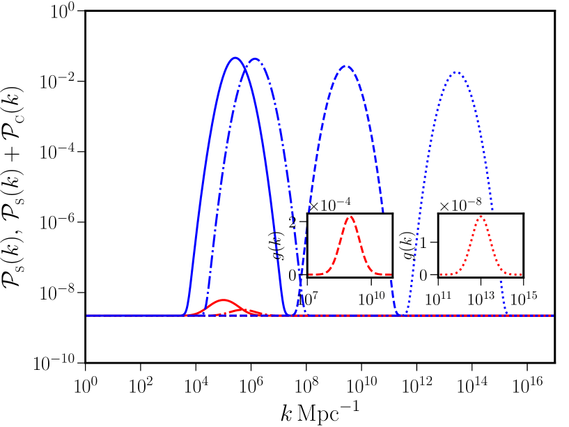
Figure 1: The scalar power spectra with a lognormal shape obtained from suitably chosen squeezed initial states have been plotted for different sets of the parameters $\gamma$ and $k_{\mathrm{f}}$ that determine the strength and the location of the peaks. Note that, we have plotted the original spectra ${\mathcal{P}}_{{}_{\mathrm{S}}}(k)$ (in red) as well as the modified spectra ${\mathcal{P}}_{{}_{\mathrm{S}}}(k)+{\mathcal{P}}_{{}_{\mathrm{C}}}(k)$ (in blue), where ${\mathcal{P}}_{{}_{\mathrm{C}}}(k)$ denotes the non-Gaussian modifications to the power spectrum [cf. eqs. (2.16) and (2.17)]. We have illustrated the spectra for the following four values of $k_{\mathrm{f}}$: $10^{5}\,{\mathrm{Mpc}}^{-1}$ (as solid curves), $5\times 10^{5}\,{\mathrm{Mpc}}^{-1}$ (as dashed-dotted curves), $10^{9}\,{\mathrm{Mpc}}^{-1}$ (as dashed curves) and $10^{13}\,{\mathrm{Mpc}}^{-1}$ (as dotted curves). We have chosen the corresponding values of $\gamma$ to be $4.5$, $1.2$, $5.5\times 10^{-4}$ and $4.5\times 10^{-8}$, respectively. We have set the width $\Delta_{k}$ of the lognormal distribution to be unity in all the cases. The features in the original spectra ${\mathcal{P}}_{{}_{\mathrm{S}}}(k)$ with peaks around $10^{9}\,{\mathrm{Mpc}}^{-1}$ and $10^{13}\,{\mathrm{Mpc}}^{-1}$ are not as discernible as those at the two other locations due to the small values of $\gamma$. Hence, in these two cases, we have included insets to highlight the function $g(k)$ [cf. eq. (2.9)] instead. The parameter $\gamma$ has been chosen so that, when the non-Gaussian modifications are taken into account, all the power spectra have roughly the same amplitudes at their peaks.

In the figure, we have also plotted the modified power spectra, i.e. ${\mathcal{P}}_{{}_{\mathrm{S}}}(k)+{\mathcal{P}}_{{}_{\mathrm{C}}}(k)$ [cf. eqs. (2.16) and (2.17)], that have been arrived at when the non-Gaussian modifications are taken into account. The reason behind the specific choice of the values for the parameter $\gamma$ will become clear when we discuss the non-Gaussian modifications to spectra in a subsequent subsection.

2.2 The associated scalar bispectrum and the non-Gaussianity parameter

We shall now proceed to calculate the corresponding scalar bispectra to eventually take into account the non-Gaussian modifications to the power spectra. In scenarios involving slow roll inflation, the scalar bispectrum, say, $G({\bm{k}}_{1},{\bm{k}}_{2},{\bm{k}}_{3})$, is known to consist of seven contributions, which arise from the cubic order action governing the scalar perturbations [56, 57, 58]. Of these seven contributions, six arise due to the bulk terms in the third order action, while the seventh arises due to a field redefinition carried out to absorb the boundary terms [59, 60]. Amongst these contributions, in the situation of interest, it is known that the first, second, third and the seventh terms, say, $G_{1}({\bm{k}}_{1},{\bm{k}}_{2},{\bm{k}}_{3})$, $G_{2}({\bm{k}}_{1},{\bm{k}}_{2},{\bm{k}}_{3})$, $G_{3}({\bm{k}}_{1},{\bm{k}}_{2},{\bm{k}}_{3})$ and $G_{7}({\bm{k}}_{1},{\bm{k}}_{2},{\bm{k}}_{3})$, dominate the contributions due to the remaining terms. Note that the three vectors ${\bm{k}}_{1}$, ${\bm{k}}_{2}$ and ${\bm{k}}_{3}$ form the edges of a triangle. As we shall discuss in the following subsection, it is the bispectrum evaluated in the so-called squeezed limit of the triangular configuration, i.e. when $k_{1}\to 0$ and $k_{2}\simeq k_{3}\simeq k$, that is expected to contribute to the non-Gaussian modifications to the power spectrum (see, for instance, refs. [61, 62, 63]).

The scalar bispectrum in slow roll inflation with squeezed initial states can be calculated easily using the de Sitter modes (2.1) describing the scalar perturbations (see, for example, refs. [42, 44, 47, 48, 49, 46]). Since the resulting expressions are somewhat lengthy, we relegate them to an appendix. We have listed the complete expressions for dominant contributions $G_{1}({\bm{k}}_{1},{\bm{k}}_{2},{\bm{k}}_{3})$, $G_{2}({\bm{k}}_{1},{\bm{k}}_{2},{\bm{k}}_{3})$, $G_{3}({\bm{k}}_{1},{\bm{k}}_{2},{\bm{k}}_{3})$ and $G_{7}({\bm{k}}_{1},{\bm{k}}_{2},{\bm{k}}_{3})$ in appendix A. It is useful to note that, in the squeezed limit, the dominant contributions to the scalar bispectrum at the wave number $k_{\mathrm{f}}$, corresponding to the location of the peak in the power spectrum ${\mathcal{P}}_{{}_{\mathrm{S}}}(k)$, can be obtained to be

$$\lim_{k_{1}\ll k_{\mathrm{f}}}k_{1}^{3}\,k_{\mathrm{f}}^{3}\,\left[G_{1}({\bm{k}}_{1},{\bm{k}}_{\mathrm{f}},-{\bm{k}}_{\mathrm{f}})+G_{3}({\bm{k}}_{1},{\bm{k}}_{\mathrm{f}},-{\bm{k}}_{\mathrm{f}})\right] = k_{1}^{3}\,k_{\mathrm{f}}^{3}\,\left[G_{1}(k_{\mathrm{f}})+G_{3}(k_{\mathrm{f}})\right]$$

$$\simeq \frac{H_{{}_{\mathrm{I}}}^{4}}{16\,M_{{}_{\mathrm{Pl}}}^{4}\,\epsilon_{1}}\,\frac{k_{\mathrm{f}}}{k_{1}}\,\frac{\gamma}{\sqrt{2\,\pi\,\Delta^{2}_{k}}}\,\left(2+\frac{\gamma}{\sqrt{2\,\pi\,\Delta^{2}_{k}}}\right),$$

$$\lim_{k_{1}\ll k_{\mathrm{f}}}k_{1}^{3}\,k_{\mathrm{f}}^{3}\,G_{2}({\bm{k}}_{1},{\bm{k}}_{\mathrm{f}},-{\bm{k}}_{\mathrm{f}}) = k_{1}^{3}\,k_{\mathrm{f}}^{3}\,G_{2}(k_{\mathrm{f}})$$

$$\simeq \frac{H_{{}_{\mathrm{I}}}^{4}}{16\,M_{{}_{\mathrm{Pl}}}^{4}\,\epsilon_{1}}\,\frac{k_{\mathrm{f}}}{k_{1}}\,\frac{\gamma}{\sqrt{2\,\pi\,\Delta^{2}_{k}}}\,\left(2+\frac{\gamma}{\sqrt{2\,\pi\,\Delta^{2}_{k}}}\right),$$

$$\lim_{k_{1}\ll k_{\mathrm{f}}}k_{1}^{3}\,k_{\mathrm{f}}^{3}\,G_{7}({\bm{k}}_{1},{\bm{k}}_{\mathrm{f}},-{\bm{k}}_{\mathrm{f}}) = k_{1}^{3}\,k_{\mathrm{f}}^{3}\,G_{7}(k_{\mathrm{f}})$$ (2.11c)

$$\simeq \frac{H_{{}_{\mathrm{I}}}^{4}\,\epsilon_{2}}{16\,M_{{}_{\mathrm{Pl}}}^{4}\,\epsilon_{1}^{2}}\,\left(1+\frac{\gamma}{\sqrt{2\,\pi\,\Delta^{2}_{k}}}\right).$$

In the above expressions, as is usually done in the context of slow roll inflation, we have combined the contributions $G_{1}(k_{\mathrm{f}})$ and $G_{3}(k_{\mathrm{f}})$, as they have a similar dependence on the wave numbers (see, for instance, ref. [60]). We should clarify that the above expressions are the dominant contributions for the values of $\gamma$ we have worked with. The striking property of the contributions $G_{1}(k_{\mathrm{f}})+G_{3}(k_{\mathrm{f}})$ and $G_{2}(k_{\mathrm{f}})$ is their dependence on the squeezed mode as $1/k_{1}$. This property of the bispectrum in case of squeezed initial states is well known [44, 46, 48]. On the other hand, note that, $G_{7}(k_{\mathrm{f}})$ is independent of $k_{1}$ in the limit $k_{1}\ll k_{\mathrm{f}}$. Therefore, at the leading order, the bispectrum around $k_{\mathrm{f}}$ is inversely proportional to the squeezed mode $k_{1}$.

Consider an observational survey extending over a certain range of scales such as, say, the measurements of the anisotropies in the CMB, which spans a few decades in wave numbers. In such a case, we can calculate the squeezed limit of the bispectrum assuming $k_{1}$ to be the smallest wave number within the range. In practice, this implies that $1\lesssim k/k_{1}\lesssim 10^{4}$ over the CMB scales. Therefore, for squeezed initial states, the bispectrum in the squeezed limit will be proportionately large and, hence, the associated non-Gaussianity parameter can be expected to be of a similar order. Note that, in this work, we are interested in examining phenomena leading to formation of PBHs and generation of secondary GWs which occur at much smaller scales. For such observations spanning several decades in wave numbers, it seems reasonable again to choose $k_{1}$ to be the smallest observable wave number. Therefore, in our calculations, we shall set the value of squeezed mode to be $k_{1}\simeq 10^{-4}\,{\mathrm{Mpc}}^{-1}$, which roughly corresponds to the Hubble scale today. Such a choice can clearly lead to a considerable enhancement in the amplitude of the scalar bispectrum and the corresponding non-Gaussianity parameter at the small scales of interest. Moreover, we should mention that, because of this boost in the amplitude, the consistency condition relating the scalar bispectrum to the power spectrum in the squeezed limit can be expected to be violated over these scales.

In figure 2, we have plotted the behavior of the bispectrum in the squeezed limit for the four set of values for the parameters of $\gamma$ and $k_{\mathrm{f}}$ we considered earlier.

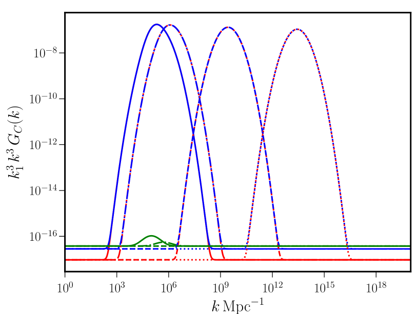
Figure 2: The dominant contributions to the dimensionless scalar bispectra in the squeezed limit, viz. $k_{1}^{3}\,k^{3}$ times $G_{1}(k)+G_{3}(k)$, $G_{2}(k)$ and $G_{7}(k)$, have been plotted (in red, blue and green, respectively) for non-vacuum initial states which lead to scalar power spectra with lognormal peaks. We have plotted the contributions to the dimensionless bispectra for the four sets of values for the parameters $\gamma$ and $k_{\mathrm{f}}$ (as solid, dashed-dotted, dashed and dotted curves) we had considered in the previous figure. It is clear that the bulk terms $G_{C}(k)$ with $C=\{1,2,3\}$ dominate the contributions to the bispectrum. In contrast, as expected, the boundary term $G_{7}(k)$ has a much smaller amplitude and mimics the shape of the power spectrum.

Notice that the amplitudes of the bispectra are significantly enhanced around the locations of the peaks in the power spectra. The amplitudes retain their slow roll values away from the peaks. The amplification of several orders of magnitude around $k_{\mathrm{f}}$ arises evidently due to the dependence of the bispectrum on the squeezed mode as $1/k_{1}$, as we discussed above. We should stress that this amplification occurs even for a relatively small value of the parameter $\gamma$, which quantifies the deviations from the Bunch-Davies vacuum. We find that, for a larger $k$, we require a smaller value of $\gamma$ to achieve the same level of enhancement of the bispectrum. In other words, the bispectrum becomes increasingly sensitive to deviations from the standard vacuum state at smaller scales.

The non-Gaussianity parameter associated with the scalar bispectrum $G({\bm{k}}_{1},{\bm{k}}_{2},{\bm{k}}_{3})$ is defined as [60, 64]

$$f_{{}_{\rm NL}}({\bm{k}}_{1},{\bm{k}}_{2},{\bm{k}}_{3}) = -\frac{10}{3}\,\frac{1}{\left(2\,\pi\right)^{4}}\;k_{1}^{3}\,k_{2}^{3}\,k_{3}^{3}\;G({\bm{k}}_{1},{\bm{k}}_{2},{\bm{k}}_{3})$$ (2.12)

$$\times\,\biggl{[}k_{1}^{3}\,{\mathcal{P}}_{{}_{\mathrm{S}}}(k_{2})\,{\mathcal{P}}_{{}_{\mathrm{S}}}(k_{3})+{\mathrm{two~{}permutations}}\biggr{]}^{-1}.$$

The dimensionless parameter $f_{{}_{\rm NL}}({\bm{k}}_{1},{\bm{k}}_{2},{\bm{k}}_{3})$ can be calculated using the expressions (2.7), (2.9) and (A.1) for the power spectrum, the function $g(k)$ and the bispectrum. In order to understand the complete shape of the scalar bispectrum, in figure 3, we have illustrated the non-Gaussianity parameter as a density plot in the $k_{1}/k_{3}$–$k_{2}/k_{3}$ plane for the first of the four sets of parameters for $\gamma$ and $k_{\mathrm{f}}$ we had introduced earlier (see the caption of figure 1).

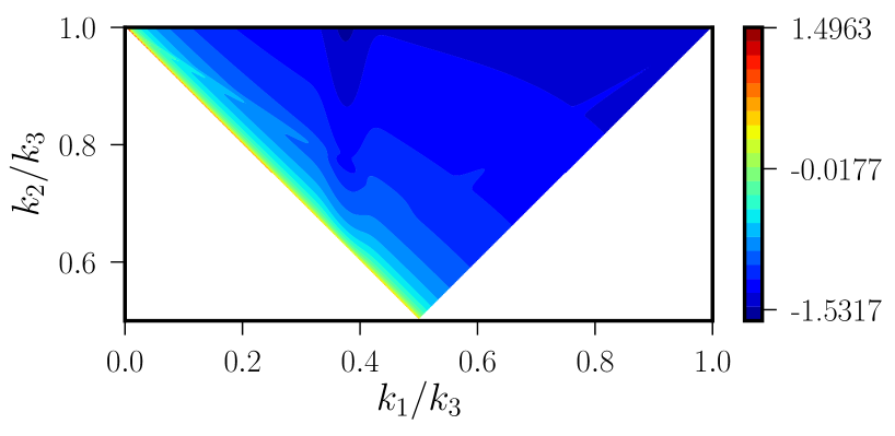
Figure 3: The non-Gaussianity parameter $\mathrm{log}\,|f_{{}_{\rm NL}}|$ has been plotted as a density plot in the $k_{1}/k_{3}$–$k_{2}/k_{3}$ plane, for the first of the four sets of parameters we had introduced in figure 1. We have set $k_{3}=k_{\mathrm{f}}$ and varied $k_{1}/k_{3}$ over the range $[5\times 10^{-4},1]$ in arriving at this figure. Note that the $f_{{}_{\rm NL}}$ parameter has a largely ‘local’ shape, with its maximum amplitude (in red) occurring in the so-called flattened limit corresponding to the left edge of the triangle.

The figure clearly illustrates the fact that the non-Gaussianity parameter has a largely ‘local’ shape. As is well known, its amplitude is the largest in the flattened limit, i.e. along the line $k_{2}/k_{3}=1-k_{1}/k_{3}$ which describes the left edge of the triangle in the figure 3. This shape evidently depends on the choice of $k_{3}$, which in this illustration has been set to be the location of the peak $k_{\mathrm{f}}$.

Let us now turn to consider the behavior of the parameter $f_{{}_{\rm NL}}$ in the squeezed limit. In such a limit, on utilizing the results (2.11), we obtain the value of $f_{{}_{\rm NL}}$ at the location of the peak in the power spectrum ${\mathcal{P}}_{{}_{\mathrm{S}}}(k)$ to be

$$\lim_{k_{1}\ll k_{\mathrm{f}}}f_{{}_{\rm NL}}^{{}^{{}_{\mathrm{SL}}}}({\bm{k}}_{1},{\bm{k}}_{\mathrm{f}},-{\bm{k}}_{\mathrm{f}})=f_{{}_{\rm NL}}^{{}^{{}_{\mathrm{SL}}}}(k_{\mathrm{f}})\simeq-\frac{5\,\epsilon_{1}}{6}\,\frac{k_{\mathrm{f}}}{k_{1}}\frac{\gamma}{\sqrt{2\,\pi\,\Delta_{k}^{2}}}\,\left(\frac{2+\frac{\gamma}{\sqrt{2\,\pi\,\Delta_{k}^{2}}}}{1+\frac{\gamma}{\sqrt{2\,\pi\,\Delta_{k}^{2}}}}\right).$$ (2.13)

In figure 4, we have plotted the behavior of $f_{{}_{\rm NL}}(k)$ in the squeezed limit for the four sets of parameters we have mentioned earlier.

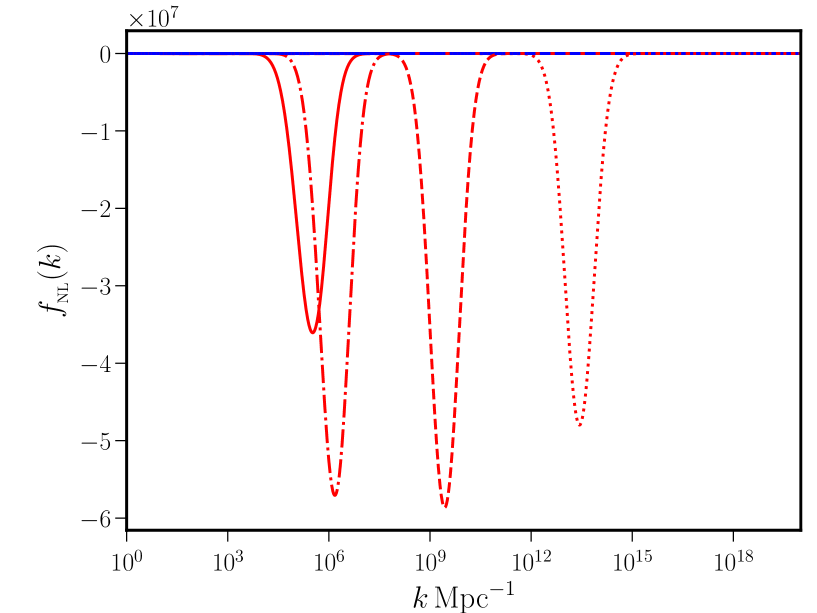
Figure 4: The non-Gaussianity parameter $f_{{}_{\rm NL}}(k)$ in the squeezed limit has been plotted (in red) for the four set of parameters (as solid, dashed-dotted, dashed and dotted curves) leading to lognormal spectra we had considered in the first two figures. We have also plotted the quantity $f_{{}_{\rm NL}}^{{}^{{}_{\mathrm{CR}}}}(k)$ (in blue) for all the cases to illustrate the fact that the consistency condition is strongly violated around the region of the peaks in the power spectra.

We find that, for these choices of the parameters, the value of $f_{{}_{\rm NL}}$ is of order $10^{7}$ around $k_{\mathrm{f}}$, while it has the slow roll value of $10^{-2}$ away from $k_{\mathrm{f}}$. Also, we find that the consistency condition — viz. that $f_{{}_{\rm NL}}^{{}^{{}_{\mathrm{CR}}}}(k)=5\,\left[n_{{}_{\mathrm{S}}}(k)-1\right]/12$, where $n_{{}_{\mathrm{S}}}(k)=1+{\rm d}\,\mathrm{ln}\,{\mathcal{P}}_{{}_{\mathrm{S}}}(k)/{\rm d}\,\mathrm{ln}\,k$ is the scalar spectral index — is strongly violated around the lognormal peak as expected, while it is satisfied sufficiently far away from the peak. It has been argued that any calculation of $f_{{}_{\rm NL}}$ has to account for the so-called local observer effect (in this context, see, for instance, refs. [65, 66]). This essentially means that, to arrive at the observable value of the non-Gaussianity parameter in the squeezed limit, we need to subtract the part of $f_{{}_{\rm NL}}$ satisfying the consistency relation from its total value. In the scenario of interest, around the peaks in the power spectra, the quantity $f_{{}_{\rm NL}}^{{}^{{}_{\mathrm{CR}}}}(k)$ is negligible compared to the magnitude of the $f_{{}_{\rm NL}}$ obtained from the squeezed initial states. The main conclusions we can draw from the above considerations are twofold. Firstly, for perturbations evolved from non-vacuum initial states, the non-Gaussianity parameter $f_{{}_{\rm NL}}$ is inversely proportional to the value of squeezed mode. Hence, it has a rather large amplitude over small scales for the values of the parameter $\gamma$ we have considered. Secondly, the amplitude of $f_{{}_{\rm NL}}$ is highly sensitive to even minor deviations from standard vacuum state. As we shall discuss in the following subsection, the large value for the non-Gaussianity parameter in the squeezed limit leads to substantial modifications to the original power spectrum. This should be contrasted with scenarios involving, say, ultra slow roll inflation, wherein the consistency condition governing the scalar bispectrum is satisfied in the squeezed limit and hence the non-Gaussian corrections to the power spectrum prove to be either negligible or identically zero [17, 38].

2.3 Non-Gaussian modifications to the scalar power spectrum

Having arrived at the bispectrum and the corresponding non-Gaussianity parameter, let us now proceed to calculate the non-Gaussian modification to the scalar power spectrum [67, 62, 63, 68, 17]. Recall that the non-Gaussianity parameter $f_{{}_{\rm NL}}$ is usually introduced through the following relation (see ref. [69]; also see, for example, refs. [60, 64]):

$${\mathcal{R}}(\eta,{\bm{x}})={\mathcal{R}}^{{}^{{}_{\mathrm{G}}}}(\eta,{\bm{x}})-\frac{3}{5}\,f_{{}_{\rm NL}}\,\left[{\mathcal{R}}^{{}^{{}_{\mathrm{G}}}}(\eta,{\bm{x}})\right]^{2},$$ (2.14)

where ${\mathcal{R}}$ is the scalar perturbation and ${\mathcal{R}}^{{}^{{}_{\mathrm{G}}}}$ denotes the Gaussian contribution. In Fourier space, this relation can be written as (see, for instance, refs. [60, 63])

$${\mathcal{R}}_{\bm{k}}={\mathcal{R}}^{{}^{{}_{\mathrm{G}}}}_{\bm{k}}-\frac{3}{5}\,f_{{}_{\rm NL}}\,\int\frac{{\rm d}^{3}{\bm{p}}}{(2\,\pi)^{3/2}}\,{\mathcal{R}}^{{}^{{}_{\mathrm{G}}}}_{\bm{p}}\;{\mathcal{R}}^{{}^{{}_{\mathrm{G}}}}_{{\bm{k}}-\bm{p}}.$$ (2.15)

If one uses this expression for ${\mathcal{R}}_{\bm{k}}$ and evaluates the corresponding two-point correlation function in Fourier space, one obtains that [62, 63, 17]

$$\langle\hat{{\mathcal{R}}}_{\bm{k}}\,\hat{{\mathcal{R}}}_{{\bm{k}}^{\prime}}\rangle=\frac{2\,\pi^{2}}{k^{3}}\,\delta^{(3)}({\bm{k}}+{\bm{k}}^{\prime})\,\left[{\mathcal{P}}_{{}_{\mathrm{S}}}(k)+\left(\frac{3}{5}\right)^{2}\,\frac{k^{3}}{2\,\pi}\,f_{{}_{\rm NL}}^{2}\,\int{\rm d}^{3}{\bm{p}}\,\frac{{\mathcal{P}}_{{}_{\mathrm{S}}}(p)}{p^{3}}\,\frac{{\mathcal{P}}_{{}_{\mathrm{S}}}\left(|{\bm{k}}-\bm{p}|\right)}{|{\bm{k}}-\bm{p}|^{3}}\right],$$ (2.16)

where ${\mathcal{P}}_{{}_{\mathrm{S}}}(k)$ is the original scalar power spectrum defined in the Gaussian limit, while the second term represents the leading non-Gaussian modifications. It can be easily shown that the non-Gaussian modification to the scalar power spectrum, say, ${\mathcal{P}}_{{}_{\mathrm{C}}}(k)$, can be expressed as

$${\mathcal{P}}_{{}_{\mathrm{C}}}(k) = \left(\frac{12}{5}\right)^{2}\,f_{{}_{\rm NL}}^{2}\,\int_{0}^{\infty}{\rm d}s\int_{0}^{1}\frac{{\rm d}d}{(s^{2}-d^{2})^{2}}\,{\mathcal{P}}_{{}_{\mathrm{S}}}[k\,(s+d)/2]\,{\mathcal{P}}_{{}_{\mathrm{S}}}[k\,(s-d)/2].$$ (2.17)

We should clarify a few points at this stage of our discussion. We should mention that the quantity $f_{{}_{\rm NL}}$ has been assumed to be local in arriving at the above expression for the correction to the power spectrum ${\mathcal{P}}_{{}_{\mathrm{C}}}(k)$. Therefore, we shall work with the value $f_{{}_{\rm NL}}$ in the squeezed limit when calculating the non-Gaussian modifications to the power spectrum. (Recall that, around $k_{\mathrm{f}}$, the scalar bispectrum had a largely ‘local’ shape, as illustrated in figure 3.) Moreover, the parameter $f_{{}_{\rm NL}}$ in the squeezed limit in our scenario is highly scale dependent in the sense that it is large around $k_{\mathrm{f}}$ (for the values of the parameter $\gamma$ we have worked with), but is completely negligible away from it. Hence, when calculating the modifications to the spectrum, in eq. (2.17), we have assumed $f_{{}_{\rm NL}}$ to be a function of $k$. In figure 1, we have plotted the modified spectra, viz. ${\mathcal{P}}_{{}_{\mathrm{S}}}(k)+{\mathcal{P}}_{{}_{\mathrm{C}}}(k)$, as well as the spectra ${\mathcal{P}}_{{}_{\mathrm{S}}}(k)$ we had originally constructed. Note that the non-Gaussian modifications ${\mathcal{P}}_{{}_{\mathrm{C}}}(k)$ dominate at small scales around the peaks in the original power spectra. In fact, it is due to the dependence of the non-Gaussianity parameter $f_{{}_{\rm NL}}$ on the squeezed mode as $1/k_{1}$ that we have been able to achieve the required boost in the power spectrum [of $\mathcal{O}(10^{-2})$] at small scales. Also, we should point out that, given a $\gamma$, the amplification due to the non-Gaussian modifications are larger at a higher $k_{\mathrm{f}}$. It is due to this reason that, for a larger $k_{\mathrm{f}}$, we have worked with a smaller value of $\gamma$. We have chosen these parameters so that, when the non-Gaussian modifications are taken into account, the modified power spectra have comparable amplitudes at their maxima despite the varying amplitudes of the peaks in their original spectra. We should clarify that the large, cubic order, non-Gaussian corrections do not lead to a breakdown of the perturbation theory since the scalar power spectra are of $\mathcal{O}(10^{-2})$ even when the modifications due to the scalar bispectra have been taken into account (cf. figure 1).

It is worthwhile to highlight another related point at this stage of our discussion. We find that the widths of the modified power spectra are larger than the widths of the original power spectra which were dictated by the parameter $\Delta_{k}$ that we have set to unity. This is because of the nature of the integrand involved that describes the non-Gaussian correction given in eq. (2.17). The appearance of the integration variables $s$ and $d$ in the arguments of the original power spectrum as well as the limits of the integrals involved contribute to the widening of the peak and a slight shift of power towards larger wave numbers in the final modified spectra.

3 Formation of PBHs and generation of secondary GWs

In this section, we shall calculate the observable quantities $f_{{}_{\mathrm{PBH}}}(M)$ and $\Omega_{{}_{\mathrm{GW}}}(f)$ using the scalar power spectra with the non-Gaussian corrections taken into account.

Given a primordial scalar power spectrum ${\mathcal{P}}_{{}_{\mathrm{S}}}(k)$, there exists a standard procedure to arrive at the corresponding $f_{{}_{\mathrm{PBH}}}(M)$ characterizing the fraction of PBHs constituting dark matter today. Let us quickly recall the essential points in this regard. We shall focus on scales that reenter the Hubble radius during the radiation dominated epoch. In such a case, the observable $f_{{}_{\mathrm{PBH}}}$ can be expressed in terms of the mass $M$ of the PBHs as follows (in this context, see the reviews [70, 71, 72, 73]):

$$f_{{}_{\mathrm{PBH}}}(M)=\left(\frac{\gamma_{\ast}}{0.2}\right)^{3/2}\,\left(\frac{\beta(M)}{1.46\times 10^{-8}}\right)\,\left(\frac{g_{\ast,k}}{g_{\ast,\mathrm{eq}}}\right)^{-1/4}\,\left(\frac{M}{M_{\odot}}\right)^{-1/2},$$ (3.1)

where $\beta(M)$ denotes the fraction of the energy density of PBHs to the total energy density of the universe at the time of their formation. The quantities $g_{\ast,k}$ and $g_{\ast,{\mathrm{eq}}}$ are the number of effective relativistic degrees of freedom at the time of formation of the PBHs and at matter-radiation equality, respectively, while $\gamma_{\ast}$ denotes the efficiency of the process leading to the formation of black holes. We shall set $g_{\ast,k}=106.75\,$, $g_{\ast,{\mathrm{eq}}}=3.36$ and $\gamma_{\ast}=0.2$, as is often done in this context. If we now assume that perturbations beyond a threshold density contrast, say, $\delta_{\mathrm{c}}$, are responsible for the formation of PBHs, then the function $\beta(M)$ is given by

$$\beta(M)\simeq\frac{1}{2}\,\left[1-\mathrm{erf}\left(\frac{\delta_{\mathrm{c}}}{\sqrt{2\,\sigma^{2}(R)}}\right)\right],$$ (3.2)

where $\mathrm{erf}(z)$ is the error function. The variance $\sigma^{2}(R)$ is related to the primordial scalar power spectrum ${\mathcal{P}}_{{}_{\mathrm{S}}}(k)$ through the integral

$$\sigma^{2}(R)=\frac{16\,R^{4}}{81}\int_{0}^{\infty}{\rm d}\,{\mathrm{ln}}k\;k^{4}\,{\mathcal{P}}_{{}_{\mathrm{S}}}(k)\,W^{2}(k,R),$$ (3.3)

where $W(k,R)$ is a window function with a smoothening radius $R$, which we shall assume to be a Gaussian of the form $W(k\,R)=\mathrm{e}^{-(k^{2}\,R^{2})/2}$. Note that the length scale $R$ is related to the mass $M$ of PBHs through the expression

$$R=4.72\times 10^{-7}\,\left(\frac{\gamma}{0.2}\right)^{-1/2}\,\left(\frac{g_{\ast,k}}{g_{\ast,\mathrm{eq}}}\right)^{1/12}\,\left(\frac{M}{M_{\odot}}\right)^{1/2}\,\mathrm{Mpc}\,.$$ (3.4)

Therefore, given a power spectrum ${\mathcal{P}}_{{}_{\mathrm{S}}}(k)$ we can first compute the variance $\sigma^{2}(R)$. We should clarify that we shall make use of the scalar power spectrum with the non-Gaussian modifications taken into account, i.e. we shall consider ${\mathcal{P}}_{{}_{\mathrm{S}}}(k)+{\mathcal{P}}_{{}_{\mathrm{C}}}(k)$. We can then make use of the above relation between $R$ and $M$ and the expression for $\beta(M)$ to finally arrive at $f_{{}_{\mathrm{PBH}}}(M)$ utilizing eq. (3.1). It is well known that the threshold of the density contrast $\delta_{\mathrm{c}}$ is a crucial parameter since $f_{{}_{\mathrm{PBH}}}$ is exponentially sensitive to it. The value of $\delta_{\mathrm{c}}$ is expected to lie in the range $0.3$–$0.65$ (see refs. [74, 75, 76, 77], see however the recent discussion [78]). For the purposes of illustration, we shall work with $\delta_{\mathrm{c}}=1/3$ and $0.5$. We should clarify that the exact value of this parameter does not affect the primary conclusions we draw about the mechanism of generating PBHs from squeezed initial states.

As we mentioned, the amplification of scalar power at small scales invariably produces secondary GWs of significant strength as they are sourced by the second order scalar perturbations [34, 33, 79, 80]. With the scalar power spectra obtained from squeezed initial states, we shall also proceed to calculate the dimensionless energy density $\Omega_{{}_{\mathrm{GW}}}$ of the secondary GWs today as a function of the frequency, say, $f$. The calculations involved are well understood [81, 82, 83, 52, 84]. We should mention here that, as we had done in the calculation of $f_{{}_{\mathrm{PBH}}}(M)$, we shall take into account the non-Gaussian modifications to the power spectrum to arrive at $\Omega_{{}_{\mathrm{GW}}}(f)$ [62, 63]. Recall that we are focusing on scales that reenter the Hubble radius during the radiation dominated epoch. In such a case, the second order tensor perturbations induced by the scalar perturbations oscillate in the sub-Hubble regime. Upon averaging over small time scales corresponding to these oscillations, the power spectrum of the secondary tensor perturbations, say, $\overline{{\mathcal{P}}_{h}(k,\eta)}$, can be expressed in terms of the scalar power spectrum as follows (see, for instance, refs. [85, 86, 87, 82]):

$$\overline{{\mathcal{P}}_{h}(k,\eta)} = \frac{2}{81\,k^{2}\,\eta^{2}}\int_{0}^{\infty}{\rm d}v\,\int_{|1-v|}^{1+v}{\rm d}u\,\left[\frac{4\,v^{2}-(1+v^{2}-u^{2})^{2}}{4\,u\,v}\right]^{2}\,{\mathcal{P}}_{{}_{\mathrm{S}}}(k\,v)\,{\mathcal{P}}_{{}_{\mathrm{S}}}(k\,u)$$ (3.5)

$$\times\,\left[{\mathcal{I}}_{c}^{2}(u,v)+{\mathcal{I}}_{s}^{2}(u,v)\right],$$

where the functions ${\mathcal{I}}_{c}(u,v)$ and ${\mathcal{I}}_{s}(u,v)$ are given by [81, 82]

$${\mathcal{I}}_{c}(v,u) = -\frac{27\,\pi}{4\,v^{3}\,u^{3}}\,\Theta\left(v+u-\sqrt{3}\right)\,(v^{2}+u^{2}-3)^{2},$$ (3.6a)

$${\mathcal{I}}_{s}(v,u) = -\frac{27}{4\,v^{3}\,u^{3}}\,(v^{2}+u^{2}-3)\,\left[4\,v\,u+(v^{2}+u^{2}-3)\;{\rm log}\,\biggl{|}\frac{3-(v-u)^{2}}{3-(v+u)^{2}}\biggr{|}\right]$$ (3.6b)

with $\Theta(z)$ denoting the step function. The dimensionless energy density associated with the secondary GWs $\Omega_{{}_{\mathrm{GW}}}(k,\eta)$, evaluated at late enough times when the modes are inside the Hubble radius during the radiation dominated epoch, is given by

$$\Omega_{{}_{\mathrm{GW}}}(k,\eta)=\frac{1}{24}\,\left(\frac{k}{{a\,H}}\right)^{2}\,\overline{{\mathcal{P}}_{h}(k,\eta)}.$$ (3.7)

The observable quantity of interest, viz. the energy density of secondary GWs evaluated today $\Omega_{{}_{\mathrm{GW}}}(f)$ (with $f$ being the frequency associated with the wave number $k$), can be written in terms of the quantity $\Omega_{{}_{\mathrm{GW}}}(k,\eta)$ above as

$$h^{2}\,\Omega_{{}_{\mathrm{GW}}}(k)\simeq 1.38\times 10^{-5}\,\left(\frac{g_{\ast,k}}{106.75}\right)^{-1/3}\,\left(\frac{\Omega_{\mathrm{r}}\,h^{2}}{4.16\times 10^{-5}}\right)\,\Omega_{{}_{\mathrm{GW}}}(k,\eta),$$ (3.8)

where $\Omega_{\mathrm{r}}$ denotes the present day dimensionless energy density of relativistic matter and $h$ is the usual parameter introduced to describe the Hubble parameter today as $H_{0}=100\,h\,\mathrm{km}\,\mathrm{s}^{-1}\,{\mathrm{Mpc}}^{-1}$.

In figure 5, we have plotted the quantities $f_{{}_{\mathrm{PBH}}}(M)$ and $\Omega_{{}_{\mathrm{GW}}}(f)$ for the four power spectra we have obtained from squeezed initial states with the non-Gaussian modifications taken into account [cf. eqs. (2.16) and (2.17)].

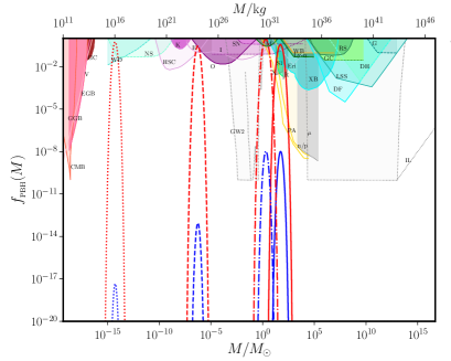
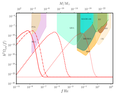
Figure 5: The quantity $f_{{}_{\mathrm{PBH}}}(M)$ (on the left, for $\delta_{\mathrm{c}}=1/3$ and $0.5$ in red and blue, respectively) and the dimensionless energy density of GWs $\Omega_{{}_{\mathrm{GW}}}(f)$ (on the right) have been plotted for the cases of the four lognormal spectra with the non-Gaussian modifications to the power spectrum taken into account that were illustrated in figure 1. The various constraints on $f_{{}_{\mathrm{PBH}}}(M)$ from different observations have also been indicated (on top of the figure on the left) over the corresponding mass ranges. We have also included the sensitivity curves of the various ongoing and upcoming observational missions of GWs (as shaded regions in the top part of the figure on the right). The intersections of the curves with the shaded regions translate to constraints on the parameter $\gamma$ which determines the extent of deviation of the initial state from the Bunch-Davies vacuum.

We have also included the constraints on $f_{{}_{\mathrm{PBH}}}(M)$ that are presently available from different datasets in the various mass ranges (see refs. [88, 70]; for recent discussions of the constraints over specific mass ranges, see refs. [89, 90]). Moreover, we have illustrated the sensitivity curves of the various GW observatories and missions (in this context, see ref. [36]). As expected, the enhancements in the scalar power on small scales lead to proportional amplifications in $f_{{}_{\mathrm{PBH}}}(M)$ and $\Omega_{{}_{\mathrm{GW}}}(f)$ over the corresponding masses and frequencies. Also, due to the nature of the integrals that determine $\overline{{\mathcal{P}}_{h}(k,\eta)}$ [cf. eq. (3.5)], the peaks of $\Omega_{{}_{\mathrm{GW}}}(f)$ are considerably wider when compared to the peaks of the scalar power spectra. As can be seen from the figure, the predicted $f_{{}_{\mathrm{PBH}}}(M)$ and $\Omega_{{}_{\mathrm{GW}}}(f)$ curves already intersect the various constraints and sensitivity curves. These constraints immediately translate to bounds on the parameter $\gamma$ which determines the strength of the feature in the scalar power spectra. Recall that, the Bogoliubov coefficient $\beta(k)$ is proportional to $\gamma$ [cf. eq. (2.10)]. So, in our scenario of PBHs and secondary GWs produced from excited initial states, evidently, the limits on $f_{{}_{\mathrm{PBH}}}$ and $\Omega_{{}_{\mathrm{GW}}}$ directly constrain the non-vacuum nature of the states from which the perturbations evolve.

4 Challenges associated with squeezed initial states

In the last two sections, we have illustrated that a specific choice for the Bogoliubov coefficient $\beta(k)$ can lead to the desired lognormal peak in the scalar power spectrum [cf. eqs. (2.7), (2.9) and (2.10)]. We have also shown that, since the cubic order non-Gaussian corrections prove to be significant in the squeezed limit in the non-vacuum initial states, it is possible to choose a relatively small value for $\beta(k)$ to arrive at large peaks in the effective scalar power spectrum. We have also examined the possible imprints of such power spectra on the extent of PBHs produced and the secondary GWs generated on small scales. In this section, we shall discuss some of the challenges associated with squeezed initial states.

4.1 Possible mechanisms to generate squeezed states

The first task before us is to justify the choice of the squeezed initial states of our interest. In other words, we need to examine whether there exist mechanisms that can generate the specific form of $\beta(k)$ that we have considered. Note that, we have assumed that the curvature perturbation is in the non-vacuum initial state at some early time, say, $\eta_{\rm i}$, when the smallest wave number of our interest, viz. $k_{1}\simeq 10^{-4}\,{\mathrm{Mpc}}^{-1}$, is adequately inside the Hubble radius. In this subsection, we shall discuss mechanisms that can possibly excite the curvature perturbations to such an initial state and the challenges associated with them.

The first possibility would be to consider effects due to high energy physics. For instance, since the large scale modes emerge from sub-Planckian length scales during the initial stages of inflation, it has been argued that trans-Planckian physics may modify the dynamics of the perturbations during the early stages (for the original discussion, see ref. [39]). But, in the absence of a viable model of quantum gravity to take into account the high energy effects, the equations describing the perturbations are often modified by hand. The modifications essentially introduce an energy scale into the equations of motion governing the perturbations, beyond which the new physics operates, while ensuring that the standard equations are satisfied at lower energies. One of the approaches that has been extensively examined in this context involves modifying the dispersion relation governing the perturbations (for example, see the review [48]). In this context, while the super-luminal dispersion relations are known to leave the primordial spectrum largely unaffected, the sub-luminal dispersion relations have been shown to lead to significant production of particles resulting in stronger features in the power spectrum [48]. However, the produced particles result in significant backreaction (a point which we shall discuss in the following subsection) making them unviable. We also find that, in some of the approaches, the power spectrum is modified on large scales, since they emerge from the sub-Planckian length scales at high energies (see, for instance, ref. [91]). Another popular method that has been considered to take into account the high energy effects involves the imposition of non-trivial initial conditions on the standard modes as they emerge from the Planckian regime [92]. Such an approach is known to only result in oscillations in the power spectrum over a wide range of scales [93, 94].

Another possibility that can leave the curvature perturbation in an excited state during the early stages of inflation would be to consider an initial epoch of non-inflationary phase. Often, one either considers a radiation dominated phase or an initial period wherein the scalar field is rolling rapidly (in this context, see, for instance, refs. [95, 96]; for recent discussions, see refs. [97, 98]). Again, in such cases, the power spectrum seems to be modified only on large scales and it often displays a sharp drop in power over these scales. Moreover, we should add that, in such scenarios, it is possible that a certain range of wave numbers would have never been inside the Hubble radius. Therefore, there can arise some ambiguity in the initial conditions that are to be imposed on these modes. Moreover, we should mention that, if such a pre-inflationary mechanism is to excite the state of the curvature perturbation at the small wave numbers $k_{\mathrm{f}}$ of interest, the mechanism should involve changes that occur as rapidly as $k_{\mathrm{f}}^{-1}$ (for a recent related discussion, see, for example, ref. [99]). Yet another possibility would be to consider two stages of slow roll inflation with either a brief departure from slow roll or even a break from inflation sandwiched between them. But, these are exactly the scenarios of ultra slow roll and punctuated inflation that have been considered to generate increased power on small scales so as to lead to enhanced formation of PBHs and higher strengths of secondary GWs [11, 16, 17, 18]). Apart from single field models, as had mentioned in the introductory section, there also exist inflationary scenarios involving two fields which can lead to a rapid rise in power on small scales [25, 27, 100]. Often, in this context, there arises a sharp turn in the trajectory of the fields, essentially giving rise to particle production and therefore a non-trivial form of $\beta(k)$ (in this context, see the discussion in ref. [27]). However, these models involve a certain level of fine tuning of the field trajectory and the form of $\beta(k)$ will be dependent on the details of the model. Importantly, we should mention that, in such cases, the features are generated as the modes of interest leave the Hubble radius during the epochs of deviations from slow roll. Actually, this is true of any inflationary scenario. This implies that it is difficult to generate features on small scales as we desire by inducing or introducing transitions in or between inflationary phases at very early stages.

In fact, there exists one more possibility. One can treat the curvature perturbation that we are considering as associated with a test field in an inflationary regime driven by another source (for scenarios wherein the dominating background is driven by another scalar field, see, for instance, refs. [101, 102]; for situations wherein the perturbations are dominated by, say, the Higgs field, see refs. [103, 82]). The source that dominates the background dynamics either prior to inflation or in the early stages of the inflationary regime can excite the modes associated with the curvature perturbations leaving it in a squeezed state. Let us illustrate the points we wish to make in this regard by starting with the aid of an example. Consider a situation wherein the Fourier mode $\psi_{k}$ of a quantum field satisfies an equation of motion of the following form:

$$\psi_{k}^{\prime\prime}+\left(k^{2}+\mu^{2}\,k_{0}^{2}\,\eta^{2}\right)\,\psi_{k}=0,$$ (4.1)

where $\mu$ and $k_{0}$ denote scales associated with the system. The solution to such a differential equation can be expressed in terms of the parabolic cylinder functions and by comparing the asymptotic forms of the solutions at early and late times, one can immediately show that the number of particles produced in such a case is given by (in this context, see the discussions in the recent work [99])

$$|\beta(k)|^{2}=\mathrm{e}^{-k^{2}/(\mu\,k_{0})}.$$ (4.2)

In fact, such a result should not come as a surprise. One encounters an equation of motion of the above form when one considers a complex scalar field that is evolving in the background of a constant electric field in flat spacetime, leading to the well known Schwinger effect [104]. Note that the above Bogoliubov coefficient (to be precise, its modulus squared) is a Gaussian, which is close to the form that we desire. However, since it is not of the lognormal shape, it is peaked at $k=0$ rather than at a non-zero $k$. Moreover, it has a maximum value of unity, whereas we require an additional parameter (such as $\gamma$) to be able to tune the amplitude of $\beta(k)$.

Let us now discuss mechanisms that can possibly help us achieve the desired $\beta(k)$ in a FLRW universe. A good starting point seems to be to construct situations in which the equation governing either the curvature perturbation or a test scalar field has the same form as eq. (4.1) above so that we can at least arrive at a Gaussian form for $|\beta(k)|^{2}$. Recall that the Mukhanov-Sasaki variable $v_{k}$ associated with the curvature perturbation satisfies the equation

$$v_{k}^{\prime\prime}+\left(k^{2}-\frac{z^{\prime\prime}}{z}\right)\,v_{k}=0,$$ (4.3)

where $z=\sqrt{2\,\epsilon_{1}}\,M_{{}_{\mathrm{Pl}}}\,a$. Evidently, we require $z^{\prime\prime}/z=-\mu^{2}\,k_{0}^{2}\,\eta^{2}$ if we are to achieve the $|\beta(k)|^{2}$ mentioned above [cf. eq. (4.2)]. In such a case, the generic solution to $z$ can be immediately expressed in terms of a linear combination of the parabolic cylinder functions (as the modes $v_{k}$ themselves can be). But, we find that the generic solution for $z$ does not remain positive definite, which is unacceptable (due to the form of $z$ quoted above). Therefore, the proposal does not seem viable. If we now instead consider a massive, test scalar field of mass $\mu$ in a radiation dominated universe, one arrives at an equation governing the modes exactly as in eq. (4.1). Interestingly, one indeed obtains a spectrum of particles as in eq. (4.2) when the evolution of massive scalar fields are examined in certain scenarios involving radiation dominated universes (in this context, see ref. [105]). If such a scenario is acceptable, there still remains the task of converting the Gaussian distribution for $|\beta(k)|^{2}$ into a lognormal distribution. Remarkably, if we replace $k^{2}$ by $f^{2}(k)$ with $f(k)=\mathrm{ln}\,(k/k_{\mathrm{f}})$, we indeed arrive at a $|\beta(k)|^{2}$ which has a lognormal shape. However, the challenge is to justify the replacement of $k^{2}$ by a generic function $f^{2}(k)$. At first sight this seems possible if we modify the dispersion relation so that $\omega^{2}(k)=k^{2}$ is replaced by $\omega^{2}(k)=f^{2}(k)$. However, note that, since the field is evolving in a FLRW universe, such a modified dispersion relation would apply to the physical wave number $k/a$ rather than to $k$ itself (in this context, see the discussion in ref. [48]). Clearly, such a choice modifies the equation (4.1) and hence the solutions completely. More importantly, as we pointed out, it has been established that strong modifications to the dispersion relation will lead to a copious amount of particle production which backreacts significantly on the background (in this context, also see the following subsection on the issue of backreaction). The above set of arguments suggests that it is rather difficult to construct mechanisms that lead to the form of $\beta(k)$ that we have worked with.

4.2 Limits due to backreaction

In this subsection, we shall discuss another challenge that arises with the squeezed initial states we have worked with. When the perturbations are evolved from non-vacuum initial states, we must ensure that the energy density associated with the excited states is less than the energy density driving the inflationary background. If the densities become comparable, then, evidently, the perturbations can start affecting the background dynamics. This issue is often referred to as the backreaction problem (see, for instance, refs. [106, 107, 41, 48, 50, 108]). We shall now arrive at constraints on the parameter $\gamma$ that determines the strength of the squeezed states by demanding that the issue of backreaction is avoided in the situation we are considering.

The task ahead is to calculate the energy density associated with the curvature perturbations when they are assumed to be in a squeezed initial state. We find that the energy density associated with the curvature perturbations in the de Sitter limit that we are considering can be expressed as follows:

$$\rho_{{}_{\mathcal{R}}} = \rho_{{}_{\mathcal{R}}}^{(1)}+\rho_{{}_{\mathcal{R}}}^{(2)}$$ (4.4)

$$\simeq \frac{1}{2\,\pi^{2}\,a^{4}}\int_{-\eta^{-1}}^{\infty}\,{\rm d}k\,k^{3}\,|\beta(k)|^{2}$$

$$+\,\frac{H_{{}_{\mathrm{I}}}^{2}}{8\,\pi^{2}\,a^{2}}\int_{0}^{-\eta^{-1}}\,dk\,k\,\biggl{\{}2\,|\beta(k)|^{2}-\left[\alpha(k)\,\beta^{\ast}(k)+\alpha^{\ast}(k)\,\beta(k)\right]\biggr{\}}.$$

where $\beta(k)$ is the Bogoliubov coefficient which indicates the extent of deviation from the Bunch-Davies vacuum. There are a couple of clarifying remarks we should make regarding this expression. Firstly, in arriving at the above expression, we have subtracted the contribution due to the Bunch-Davies vacuum, which, upon regularization, is known to correspond to (see, for example, refs. [109, 110])

$$\rho_{{}_{\mathcal{R}}}^{{}_{\mathrm{BD}}}=\frac{61\,H_{{}_{\mathrm{I}}}^{4}}{960\,\pi^{4}}.$$ (4.5)

Clearly, this is sub-dominant to the background energy density which behaves as $\rho_{{}_{\mathrm{I}}}=3\,H_{{}_{\mathrm{I}}}^{2}\,M_{{}_{\mathrm{Pl}}}^{2}$ (since $H_{{}_{\mathrm{I}}}/M_{{}_{\mathrm{Pl}}}<10^{-5}$). Secondly, it should be evident that we have divided the total energy density into two parts, with the first part $\rho_{{}_{\mathcal{R}}}^{(1)}$ arising from the contributions due to the modes that are in the sub-Hubble domain at any instance, while the second part $\rho_{{}_{\mathcal{R}}}^{(2)}$ corresponds to modes that are in the super-Hubble domain. At early times, when all the modes are well inside the Hubble radius, it is the first part that dominates (in this context, see, for instance, refs. [41, 49]). This result can be easily understood in simple instances such as, say, power law inflation. In such cases, as is well known, the curvature perturbation behaves in a manner similar to that of a massless scalar field. The expression $\rho_{{}_{\mathcal{R}}}^{(1)}$ is essentially the same as the energy density of a massless scalar field in the sub-Hubble limit. Note that the energy density $\rho_{{}_{\mathcal{R}}}^{(1)}$ behaves as $a^{-4}$. In other words, the energy density is the largest at early times when the initial conditions are imposed on the modes of interest in the sub-Hubble regime. We shall soon see that this behavior severely restricts the amplitude of the parameter $\gamma$.

As we discussed above, it is the sub-Hubble contribution $\rho_{{}_{\mathcal{R}}}^{(1)}$ that dominates in the expression (4.4) for $\rho_{{}_{\mathcal{R}}}$ at early times. Recall that, in the scenario we are considering, $\beta(k)$ is determined by the lognormal function $g(k)$ [cf. eqs. (2.9) and (2.10)] that describes the feature in the scalar power spectrum. Since $g(k)$ is a Gaussian with the strength $\gamma$ at its maximum [cf. eq. (2.9)], we have $g(k)\lesssim\gamma$ for all $k$. We have always worked with values such that $\gamma\lesssim{\cal O}(1)$. Therefore, we can approximate the expression for $\beta(k)$ that is to be used in the integral describing $\rho_{{}_{\mathcal{R}}}^{(1)}$ [cf. eq. (4.4)] as $\beta(k)\simeq-g(k)/2$. This simplifies the evaluation of $\rho_{{}_{\mathcal{R}}}^{(1)}$, and we obtain the energy density of the perturbations in terms of the parameters $\gamma$, $k_{\mathrm{f}}$ and $\Delta_{k}$ to be

$$\rho_{{}_{\mathcal{R}}}\simeq\rho_{{}_{\mathcal{R}}}^{(1)}\simeq\frac{\gamma^{2}\,\mathrm{e}^{4\,\Delta_{k}^{2}}}{16\,\pi^{5/2}\,\Delta_{k}}\,\left(\frac{k_{\mathrm{f}}}{a}\right)^{4}.$$ (4.6)

We should stress again that we have subtracted the contribution due to the Bunch-Davies vacuum in arriving at this expression. Due to this reason, we should also add that no regularization is required to arrive at the above result. Hence, $\rho_{{}_{\mathcal{R}}}\to 0$ when $\gamma\to 0$, as expected. We find that the relative difference between the above approximate estimate of $\rho_{{}_{\cal R}}^{(1)}$ [obtained by assuming that $\beta(k)\simeq-g(k)/2$] and the exact estimate is at most of $\mathcal{O}(1)$. Therefore, for convenience, we shall use the approximate estimate to arrive at the bound on the parameter $\gamma$ in our scenario.

For the backreaction to be negligible in our scenario, we require that $\rho_{{}_{\mathcal{R}}}\ll\rho_{{}_{\mathrm{I}}}$, where, as we mentioned, $\rho_{{}_{\mathrm{I}}}=3\,H_{{}_{\mathrm{I}}}^{2}\,M_{{}_{\mathrm{Pl}}}^{2}$ is the energy density of the background during inflation. This requirement leads to the condition

$$\frac{\gamma^{2}\,\mathrm{e}^{4\,\Delta_{k}^{2}}}{\Delta_{k}}\,\left(\frac{k_{\mathrm{f}}}{a\,H_{{}_{\mathrm{I}}}}\right)^{4}\ll 48\,\pi^{5/2}\,\left(\frac{M_{{}_{\mathrm{Pl}}}}{H_{{}_{\mathrm{I}}}}\right)^{2}.$$ (4.7)

During inflation, the value of the Hubble parameter $H_{{}_{\mathrm{I}}}$ is related to the tensor-to-scalar ratio $r$ through the relation $(H_{{}_{\mathrm{I}}}/M_{{}_{\mathrm{Pl}}})^{2}\simeq r\,A_{{}_{\mathrm{S}}}$, where $A_{{}_{\mathrm{S}}}\simeq 2.11\times 10^{-9}$ is the COBE normalized scalar amplitude over the CMB scales. Since the energy density $\rho_{{}_{\mathcal{R}}}$ is the largest at early times, let us evaluate it at the time when the smallest wave number of interest, say, $k_{\mathrm{min}}$, leaves the Hubble radius, i.e. when $k_{\mathrm{min}}=a_{\mathrm{min}}\,H_{{}_{\mathrm{I}}}$. At such a time, as we have set $\Delta_{k}=1$, the above inequality reduces to (upon ignoring the constant coefficients)

$$\gamma\ll\frac{10^{9/2}}{\sqrt{r}}\,\,\left(\frac{k_{\mathrm{min}}}{k_{\mathrm{f}}}\right)^{2}.$$ (4.8)

It seems reasonable to set $k_{\mathrm{min}}=k_{1}/10\simeq 10^{-5}\,{\mathrm{Mpc}}^{-1}$ (recall that we had earlier chosen $k_{1}=10^{-4}\,{\mathrm{Mpc}}^{-1}$). If we choose $k_{\mathrm{f}}=10^{5}\,{\mathrm{Mpc}}^{-1}$, which is the smallest of the values for $k_{\mathrm{f}}$ that we had considered, then we arrive at $\gamma\ll 10^{-16.5}/\sqrt{r}$. In other words, for $r\simeq 10^{-3}$, we require $\gamma<10^{-15}$. For a larger $k_{\mathrm{f}}$, clearly, the limits on $\gamma$ are even stronger. If $k_{\mathrm{f}}\simeq 10^{13}\,{\mathrm{Mpc}}^{-1}$ and $r\simeq 10^{-3}$, we require that $\gamma<10^{-30}$. Evidently, $\gamma$ can be larger if the tensor-to-scalar ratio is smaller, i.e. when the scale of inflation is lower. Nevertheless, even for an extreme value of $r\simeq 10^{-30}$ as suggested by the recent arguments based on the trans-Planckian censorship conjecture (in this context, see, for instance, ref. [111]), we require $\gamma<10^{-2}$ for $k_{\mathrm{f}}\simeq 10^{5}\,{\mathrm{Mpc}}^{-1}$ and $\gamma<10^{-17}$ for $k_{\mathrm{f}}\simeq 10^{13}\,{\mathrm{Mpc}}^{-1}$. We have instead worked with $\gamma\simeq 1$ for $k_{\mathrm{f}}=10^{5}\,{\mathrm{Mpc}}^{-1}$ and $\gamma\simeq 10^{-8}$ for $k_{\mathrm{f}}=10^{13}\,{\mathrm{Mpc}}^{-1}$. Clearly, for a more reasonable $r$, the constraints on $\gamma$ are considerably more severe. Under such conditions, $f_{{}_{\rm NL}}$ and hence the non-Gaussian modifications will prove to be small and we will not be able to achieve the desired level of amplification of the corrected power spectrum ${\mathcal{P}}_{{}_{\mathrm{S}}}(k)+{\mathcal{P}}_{{}_{\mathrm{C}}}(k)$. In fact, $\gamma$ is so tightly constrained by the backreaction that we are essentially left with the slow roll results.

There are two related points we wish to make here. Firstly, one may wonder if the energy associated with the curvature perturbation $\rho_{{}_{\mathcal{R}}}$ itself may support accelerated expansion. Since $\rho_{{}_{\mathcal{R}}}^{(1)}\propto a^{-4}$, conservation of energy suggests that, at early times, the pressure associated with the excited states should be given by $p_{{}_{\mathcal{R}}}^{(1)}=\rho_{{}_{\mathcal{R}}}^{(1)}/3$. Upon explicit calculation, we find that this is indeed the case (in this context, also see refs. [49, 50]). In other words, the pressure associated with the excited initial states does not possess the equation of state required to drive inflation. Secondly, since the energy density of the perturbations $\rho_{{}_{\mathcal{R}}}^{(1)}$ dies down as $a^{-4}$, one may imagine that it could decay rapidly enough permitting the background energy density to dominate. Given $\rho_{{}_{\mathcal{R}}}$ at $a=a_{\mathrm{min}}$, we find that the number of e-folds after which the energy density associated with the perturbations becomes sub-dominant to $\rho_{{}_{\mathrm{I}}}$ is given by

$$N\simeq\frac{1}{4}\,\mathrm{ln}\left(\frac{\gamma^{2}\,r}{10^{9}}\right)+\mathrm{ln}\left(\frac{k_{\mathrm{f}}}{k_{\mathrm{min}}}\right).$$ (4.9)

For the values of the various quantities we have worked with, say, $\gamma\simeq 1$, $k_{\mathrm{f}}=10^{5}\,{\mathrm{Mpc}}^{-1}$ and $k_{\mathrm{min}}=10^{-5}\,{\mathrm{Mpc}}^{-1}$, if we choose a tensor-to-scalar ratio of $r\simeq 10^{-3}$, we find that it will take as many as $16$ e-folds before the background energy density begins to dominate. This duration will be more prolonged for larger values of $k_{\mathrm{f}}$. Clearly, backreaction is a rather serious issue that needs to be accounted for.

5 Conclusions

In this work, we had explored a possible mechanism for the production of PBHs and GWs wherein the primordial scalar perturbations were evolved from squeezed initial states. The advantage of the mechanism is the fact that it is completely independent of the actual model that drives the background dynamics during inflation. All we require is typical slow roll inflation which leads to a power spectrum that is consistent with the recent CMB data on large scales. By choosing specific forms for the Bogoliubov coefficients that characterize the squeezed states, we had constructed scalar power spectra with a lognormal feature at small scales. It is well known that, in such cases, the scalar bispectra in the squeezed limit is inversely proportional to the value of the squeezed mode, a dependence which we expected to utilize so that we obtain significantly high values for the scalar non-Gaussianity parameter $f_{{}_{\rm NL}}$ at large wave numbers. We had hoped that this property can lead to large non-Gaussian modifications to the scalar power spectrum, which in turn can amplify the power considerably at small scales. While the proposal seemed feasible, there were two challenges that we had encountered. Mathematically, it was rather easy to construct squeezed initial states that led to a sharp rise in power on small scales, when the non-Gaussian modifications were taken into account. However, we had found that it can be a challenge to design scenarios that excite the curvature perturbation to such an initial state during the early stages of inflation. Moreover, we had found that the backreaction on the inflationary background due to the excited state of the perturbations strongly limits the extent of deviation from the Bunch-Davies vacuum. In fact, the bounds due to the backreaction are so strong that the slow roll results remain valid.

Let us make a few further clarifying remarks at this stage of our discussion. The consistency condition relating the bispectrum and the power spectrum is known to be violated for modes that evolve from the non-vacuum initial states (i.e. around the peaks in the original power spectra). As a result, we had expected that the contributions to the non-Gaussianity parameter due to the so-called local observer effect that has to be subtracted will be small when compared to the actual value $f_{{}_{\rm NL}}$ over these wave numbers (in this context, see refs. [65, 66]). Motivated by the largely local form of the scalar bispectrum in the squeezed limit, we had utilized the corresponding $f_{{}_{\rm NL}}$ to calculate the non-Gaussian modifications to the power spectrum [61, 62, 63, 17]. We had hoped that the non-Gaussian modifications will dominate leading to enhanced power at small scales. However, we had found that the issue of backreaction put paid to the proposal.

Before we conclude, we would like to comment on four issues and their possible resolutions in the approach of generating PBHs and GWs from squeezed initial states.

1. Note that we have arrived at the scalar bispectrum by calculating the integrals involved over the domain $-\infty<\eta<0$. In other words, we have assumed that the initial squeezed state was chosen in the infinite past, i.e. as $\eta\to-\infty$. It may be argued that if we choose to work with non-vacuum initial states, then the initial conditions need to be imposed at a finite initial time, say, $\eta_{\mathrm{i}}$. We believe that our results and conclusions will hold as long as $\eta_{\mathrm{i}}\ll-1/k_{\mathrm{min}}$, where, recall that, we have set $k_{\mathrm{min}}\simeq k_{1}/10$, with $k_{1}$ being the smallest wave number of observational interest, which we have assumed to be $10^{-4}\,{\mathrm{Mpc}}^{-1}$.

2. The method by which we have calculated modifications to the power spectrum due to the scalar non-Gaussianity parameter is strictly valid for an $f_{{}_{\rm NL}}$ of the local type. In other words, $f_{{}_{\rm NL}}$ ought to be a constant independent of scale. However, in our scenario, the $f_{{}_{\rm NL}}$ we obtain is strongly scale dependent. There are two points that we believe support the method we have adopted. Firstly, in order to mimic the local behavior of $f_{{}_{\rm NL}}$, we have chosen to work with its value in the squeezed limit (in this context, also see ref. [61]). Secondly, and interestingly, we find that, near the wave numbers corresponding to the peaks of the power spectra, the non-Gaussianity parameter $f_{{}_{\rm NL}}$ seems to have a strongly local shape. We should add here that a formal approach to arrive at the modifications to the power spectrum would be to calculate the loop corrections at the appropriate order. While such an effort seems worthwhile, we believe that, since the parameter $f_{{}_{\rm NL}}$ is largely local around the maximum in the power spectrum, our calculations can be considered to be fairly suggestive.

3. In our approach, we have accounted for the cubic order non-Gaussianities by considering the corresponding modifications to the scalar power spectrum. This approach seems adequate to account for the non-Gaussian modifications to the density parameter $\Omega_{{}_{\mathrm{GW}}}$ describing the stochastic GW background [67, 62, 63]. However, when calculating the density of PBHs formed, the non-Gaussianities are expected to also modify the probability distribution of the density contrast and hence the number of PBHs at the time of their formation [cf. eq. (3.2)]. We should mention that this effect needs to be accounted for separately [112].

4. Lastly, it may be interesting to explore if the contributions due to the higher order correlations such as the trispectrum may rescue our proposal and lead to large non-Gaussian modifications despite the strong constraints on $\gamma$ due to the backreaction [113, 68]. For instance, we had seen that, in the squeezed limit, $f_{{}_{\rm NL}}$ had behaved as $k_{\mathrm{f}}/k_{1}$. If the non-Gaussianity parameter, say, $\tau_{{}_{\mathrm{NL}}}$, characterizing the trispectrum (in this context, see ref. [114]) in a squeezed initial state behaves in a stronger fashion, it seems possible that the higher order terms may modify the power spectrum adequately to circumvent the limits on $\gamma$. However, even if this works out, one concern would remain. We had seen that, despite the large value of $f_{{}_{\rm NL}}$, the amplitude of the modified power spectrum was of the order of $10^{-2}$ (for the original values of $\gamma$ we had worked with). If the non-Gaussian modifications due to the trispectrum prove to be significant, it is possible that these higher order contributions will also affect the validity of perturbation theory. One will have to ensure that the amplitude of the corrected power spectrum remains smaller than unity even when further contributions are taken into account. Probably, the conditions for the validity of the perturbation theory at higher orders would severely restrict the extent of deviations from the Bunch-Davies vacuum. We are currently exploring these issues.

We would like to close by pointing out that, the various arguments we have considered in this work suggest that the initial state of the curvature perturbations is likely to be remarkably close to the Bunch-Davies vacuum, in particular, on small scales.

Appendix A The dominant contributions to the scalar bispectrum

In this appendix, we shall provide the complete expressions describing the dominant contributions to the scalar bispectrum evaluated in a squeezed initial state. For a generic $\alpha(k)$ and $\beta(k)$, these contributions are given by the following expressions (in this context, see for example, refs. [42, 46, 48, 49]):

$$G_{1}({\bm{k}}_{1},{\bm{k}}_{2},{\bm{k}}_{3}) = \frac{H_{{}_{\mathrm{I}}}^{4}}{32\,M_{{}_{\mathrm{Pl}}}^{4}\,\epsilon_{1}}\,\frac{|\alpha_{1}|^{2}\,|\alpha_{2}|^{2}\,|\alpha_{3}|^{2}}{k_{1}\,k_{2}\,k_{3}}\frac{(1-\delta_{1})\,(1-\delta_{2})\,(1-\delta_{3})}{k_{1}^{2}}\,$$ (A.1a)

$$\times\,\Biggl{[}\frac{1+\delta^{\ast}_{1}\,\delta^{\ast}_{2}\,\delta^{\ast}_{3}}{k_{{}_{\mathrm{T}}}}\,\left(1+\frac{k_{1}}{k_{{}_{\mathrm{T}}}}\right)+\frac{\delta^{\ast}_{1}+\delta^{\ast}_{2}\,\delta^{\ast}_{3}}{k_{1}-k_{2}-k_{3}}\,\left(1+\frac{k_{1}}{k_{1}-k_{2}-k_{3}}\right)$$

$$+\,\frac{\delta^{\ast}_{2}+\delta^{\ast}_{1}\,\delta^{\ast}_{3}}{k_{2}-k_{1}-k_{3}}\left(1-\frac{k_{1}}{k_{2}-k_{1}-k_{3}}\right)+\frac{\delta^{\ast}_{3}+\delta^{\ast}_{1}\,\delta^{\ast}_{2}}{k_{3}-k_{1}-k_{2}}\left(1-\frac{k_{1}}{k_{3}-k_{1}-k_{2}}\right)\Biggr{]}$$

$$+\,\mathrm{complex~{}conjugate}+\mathrm{two~{}permutations},$$

$$G_{2}({\bm{k}}_{1},{\bm{k}}_{2},{\bm{k}}_{3}) = -\frac{H_{{}_{\mathrm{I}}}^{4}}{64\,M_{{}_{\mathrm{Pl}}}^{4}\,\epsilon_{1}}\,\frac{(k_{1}^{2}+k_{2}^{2}+k_{3}^{2})}{(k_{1}\,k_{2}\,k_{3})^{3}}\,|\alpha_{1}|^{2}\,|\alpha_{2}|^{2}\,|\alpha_{3}|^{2}\,\left(1-\delta_{1}\right)\,\left(1-\delta_{2}\right)\,\left(1-\delta_{3}\right)$$ (A.1b)

$$\times\,\Biggl{\{}\Bigg{[}\frac{i}{\eta_{\rm e}}\,\Biggl{(}\mathrm{e}^{i\,k_{{}_{\mathrm{T}}}\,\eta_{\rm e}}-\delta^{\ast}_{1}\,\mathrm{e}^{i\,(-k_{1}+k_{2}+k_{3})\,\eta_{\rm e}}-\delta^{\ast}_{2}\,\mathrm{e}^{i\,(k_{1}-k_{2}+k_{3})\,\eta_{\rm e}}-\delta^{\ast}_{3}\,\mathrm{e}^{i\,(k_{1}+k_{2}-k_{3})\,\eta_{\rm e}}$$

$$+\,\delta^{\ast}_{2}\,\delta^{\ast}_{3}\,\mathrm{e}^{-i\,(-k_{1}+k_{2}+k_{3})\,\eta_{\rm e}}+\delta^{\ast}_{1}\,\delta^{\ast}_{3}\,\mathrm{e}^{-i\,(k_{1}-k_{2}+k_{3})\,\eta_{\rm e}}+\delta^{\ast}_{1}\,\delta^{\ast}_{2}\,\mathrm{e}^{-i\,(k_{1}+k_{2}-k_{3})\,\eta_{\rm e}}$$

$$-\,\delta^{\ast}_{1}\,\delta^{\ast}_{2}\,\delta^{\ast}_{3}\,\mathrm{e}^{-i\,k_{{}_{\mathrm{T}}}\,\eta_{\rm e}}\Biggr{)}\Biggr{]}_{\eta_{\rm e}\to 0}+\,\left(1+\delta^{\ast}_{1}\,\delta^{\ast}_{2}\,\delta^{\ast}_{3}\right)\,\frac{(k_{1}\,k_{2}+k_{2}\,k_{3}+k_{1}\,k_{3})}{k_{{}_{\mathrm{T}}}}$$

$$+\,\left(\delta^{\ast}_{1}+\delta^{\ast}_{2}\,\delta^{\ast}_{3}\right)\,\frac{(k_{1}\,k_{2}-k_{2}\,k_{3}+k_{1}\,k_{3})}{(-k_{1}+k_{2}+k_{3})}$$

$$+\,\left(\delta^{\ast}_{2}+\delta^{\ast}_{1}\,\delta^{\ast}_{3}\right)\,\frac{(k_{1}\,k_{2}+k_{2}\,k_{3}-k_{1}\,k_{3})}{(k_{1}-k_{2}+k_{3})}$$

$$+\,\left(\delta^{\ast}_{3}+\delta^{\ast}_{1}\,\delta^{\ast}_{2}\right)\,\frac{(-k_{1}\,k_{2}+k_{2}\,k_{3}+k_{3}\,k_{1})}{(k_{1}+k_{2}-k_{3})}$$

$$+\,k_{1}\,k_{2}\,k_{3}\,\Biggl{[}\frac{1+\delta^{\ast}_{1}\,\delta^{\ast}_{2}\,\delta^{\ast}_{3}}{k_{{}_{\mathrm{T}}}^{2}}+\frac{(\delta^{\ast}_{1}+\delta^{\ast}_{2}\,\delta^{\ast}_{3})}{(-k_{1}+k_{2}+k_{3})^{2}}+\frac{(\delta^{\ast}_{2}+\delta^{\ast}_{1}\,\delta^{\ast}_{3})}{(k_{1}-k_{2}+k_{3})^{2}}$$

$$+\,\frac{(\delta^{\ast}_{3}+\delta^{\ast}_{1}\delta^{\ast}_{2})}{(k_{1}+k_{2}-k_{3})^{2}}\Biggr{]}+\mathrm{complex~{}conjugate},$$

$$G_{3}({\bm{k}}_{1},{\bm{k}}_{2},{\bm{k}}_{3}) = -\frac{H_{{}_{\mathrm{I}}}^{4}}{32\,M_{{}_{\mathrm{Pl}}}^{4}\,\epsilon_{1}}\,\frac{|\alpha_{1}|^{2}\,|\alpha_{2}\,|^{2}\,|\alpha_{3}|^{2}}{k_{1}\,k_{2}\,k_{3}}\,\frac{(1-\delta_{1})\,(1-\delta_{2})\,(1-\delta_{3})}{k_{1}^{2}}$$ (A.1c)

$$\times\,\frac{(k_{2}^{2}-k_{3}^{2})^{2}-k_{1}^{2}\,(k_{2}^{2}+k_{3}^{2})}{2\,k_{2}^{2}\,k_{3}^{2}}$$

$$\times\,\Biggl{[}\frac{1+\delta^{\ast}_{1}\,\delta^{\ast}_{2}\,\delta^{\ast}_{3}}{k_{{}_{\mathrm{T}}}}\,\left(1+\frac{k_{1}}{k_{{}_{\mathrm{T}}}}\right)+\frac{\delta^{\ast}_{1}+\delta^{\ast}_{2}\,\delta^{\ast}_{3}}{k_{1}-k_{2}-k_{3}}\,\left(1+\frac{k_{1}}{k_{1}-k_{2}-k_{3}}\right)$$

$$+\,\frac{\delta^{\ast}_{2}+\delta^{\ast}_{1}\,\delta^{\ast}_{3}}{k_{2}-k_{1}-k_{3}}\left(1-\frac{k_{1}}{k_{2}-k_{1}-k_{3}}\right)+\frac{\delta^{\ast}_{3}+\delta^{\ast}_{1}\,\delta^{\ast}_{2}}{k_{3}-k_{1}-k_{2}}\left(1-\frac{k_{1}}{k_{3}-k_{1}-k_{2}}\right)\Biggr{]}$$

$$+\,\mathrm{complex~{}conjugate}+\mathrm{two~{}permutations},$$

$$G_{7}({\bm{k}}_{1},{\bm{k}}_{2},{\bm{k}}_{3}) = \frac{H_{{}_{\mathrm{I}}}^{4}\,\epsilon_{2}}{32\,M_{{}_{\mathrm{Pl}}}^{4}\epsilon_{1}^{2}}\,\biggl{\{}\frac{1}{(k_{1}\,k_{2})^{3}}\,|\alpha_{1}|^{2}\,|\alpha_{2}|^{2}\,\left(1-\delta_{1}\right)\,\left(1-\delta^{\ast}_{1}\right)\,\left(1-\delta_{2}\right)\,\left(1-\delta^{\ast}_{2}\right)$$ (A.1d)

$$+\,{\rm two~{}permutations}\biggr{\}},$$

where $k_{{}_{\mathrm{T}}}=k_{1}+k_{2}+k_{3}$ and, for convenience, we have set $\alpha(k_{i})=\alpha_{i}$ and $\delta(k_{i})=\delta_{i}$ for $i=\{1,2,3\}$. Note that, we can write

$$|\alpha(k)|^{2}=\left[1-|\delta(k)|^{2}\right]^{-1}$$ (A.2)

so that the complete bispectrum can be expressed in terms of the function $\delta(k)$, which in turn is determined by the feature $g(k)$ in the power spectrum [cf. eqs. (2.7) and (2.8)].

References

- [1] B. J. Carr and S. W. Hawking, Black holes in the early Universe, Mon. Not. Roy. Astron. Soc. 168 (1974) 399–415.
- [2] B. J. Carr, The Primordial black hole mass spectrum, Astrophys. J. 201 (1975) 1–19.
- [3] LIGO Scientific, Virgo Collaboration, B. P. Abbott et al., GW151226: Observation of Gravitational Waves from a 22-Solar-Mass Binary Black Hole Coalescence, Phys. Rev. Lett. 116 (2016), no. 24 241103, [arXiv:1606.04855].
- [4] LIGO Scientific, VIRGO Collaboration, B. P. Abbott et al., GW170104: Observation of a 50-Solar-Mass Binary Black Hole Coalescence at Redshift 0.2, Phys. Rev. Lett. 118 (2017), no. 22 221101, [arXiv:1706.01812]. [Erratum: Phys. Rev. Lett.121,no.12,129901(2018)].
- [5] LIGO Scientific, Virgo Collaboration, B. P. Abbott et al., GW170608: Observation of a 19-solar-mass Binary Black Hole Coalescence, Astrophys. J. Lett. 851 (2017) L35, [arXiv:1711.05578].
- [6] LIGO Scientific, Virgo Collaboration, R. Abbott et al., GW190521: A Binary Black Hole Merger with a Total Mass of , Phys. Rev. Lett. 125 (2020), no. 10 101102, [arXiv:2009.01075].
- [7] B. Carr, K. Kohri, Y. Sendouda, and J. Yokoyama, Constraints on Primordial Black Holes, arXiv:2002.12778.
- [8] V. Domcke, F. Muia, M. Pieroni, and L. T. Witkowski, PBH dark matter from axion inflation, JCAP 07 (2017) 048, [arXiv:1704.03464].
- [9] J. Garcia-Bellido and E. Ruiz Morales, Primordial black holes from single field models of inflation, Phys. Dark Univ. 18 (2017) 47–54, [arXiv:1702.03901].
- [10] G. Ballesteros and M. Taoso, Primordial black hole dark matter from single field inflation, Phys. Rev. D 97 (2018), no. 2 023501, [arXiv:1709.05565].
- [11] C. Germani and T. Prokopec, On primordial black holes from an inflection point, Phys. Dark Univ. 18 (2017) 6–10, [arXiv:1706.04226].
- [12] I. Dalianis, A. Kehagias, and G. Tringas, Primordial black holes from -attractors, JCAP 01 (2019) 037, [arXiv:1805.09483].
- [13] S. Chongchitnan and G. Efstathiou, Accuracy of slow-roll formulae for inflationary perturbations: implications for primordial black hole formation, JCAP 01 (2007) 011, [astro-ph/0611818].
- [14] P. Pina Avelino, Primordial black hole constraints on non-gaussian inflation models, Phys. Rev. D 72 (2005) 124004, [astro-ph/0510052].
- [15] K. Inomata, M. Kawasaki, K. Mukaida, Y. Tada, and T. T. Yanagida, Inflationary Primordial Black Holes as All Dark Matter, Phys. Rev. D96 (2017), no. 4 043504, [arXiv:1701.02544].
- [16] N. Bhaumik and R. K. Jain, Primordial black holes dark matter from inflection point models of inflation and the effects of reheating, arXiv:1907.04125. [JCAP2001,037(2020)].
- [17] H. V. Ragavendra, P. Saha, L. Sriramkumar, and J. Silk, PBHs and secondary GWs from ultra slow roll and punctuated inflation, arXiv:2008.12202.
- [18] N. Bhaumik and R. K. Jain, Stochastic induced gravitational waves and lowest mass limit of primordial black holes with the effects of reheating, arXiv:2009.10424.
- [19] V. Atal, J. Garriga, and A. Marcos-Caballero, Primordial black hole formation with non-Gaussian curvature perturbations, JCAP 09 (2019) 073, [arXiv:1905.13202].
- [20] S. S. Mishra and V. Sahni, Primordial Black Holes from a tiny bump/dip in the Inflaton potential, JCAP 04 (2020) 007, [arXiv:1911.00057].
- [21] A. Y. Kamenshchik, A. Tronconi, T. Vardanyan, and G. Venturi, Non-Canonical Inflation and Primordial Black Holes Production, Phys. Lett. B791 (2019) 201–205, [arXiv:1812.02547].
- [22] G. Ballesteros, J. Beltran Jimenez, and M. Pieroni, Black hole formation from a general quadratic action for inflationary primordial fluctuations, JCAP 06 (2019) 016, [arXiv:1811.03065].
- [23] G. A. Palma, S. Sypsas, and C. Zenteno, Seeding primordial black holes in multifield inflation, Phys. Rev. Lett. 125 (2020), no. 12 121301, [arXiv:2004.06106].
- [24] J. Fumagalli, S. Renaux-Petel, J. W. Ronayne, and L. T. Witkowski, Turning in the landscape: a new mechanism for generating Primordial Black Holes, arXiv:2004.08369.
- [25] M. Braglia, D. K. Hazra, F. Finelli, G. F. Smoot, L. Sriramkumar, and A. A. Starobinsky, Generating PBHs and small-scale GWs in two-field models of inflation, JCAP 08 (2020) 001, [arXiv:2005.02895].
- [26] Z. Zhou, J. Jiang, Y.-F. Cai, M. Sasaki, and S. Pi, Primordial black holes and gravitational waves from resonant amplification during inflation, arXiv:2010.03537.
- [27] J. Fumagalli, S. Renaux-Petel, and L. T. Witkowski, Oscillations in the stochastic gravitational wave background from sharp features and particle production during inflation, arXiv:2012.02761.
- [28] Y.-F. Cai, X. Tong, D.-G. Wang, and S.-F. Yan, Primordial Black Holes from Sound Speed Resonance during Inflation, Phys. Rev. Lett. 121 (2018), no. 8 081306, [arXiv:1805.03639].
- [29] C. Chen and Y.-F. Cai, Primordial black holes from sound speed resonance in the inflaton-curvaton mixed scenario, JCAP 10 (2019) 068, [arXiv:1908.03942].
- [30] A. E. Romano, Sound speed induced production of primordial black holes, arXiv:2006.07321.
- [31] B. Carr, K. Dimopoulos, C. Owen, and T. Tenkanen, Primordial Black Hole Formation During Slow Reheating After Inflation, Phys. Rev. D 97 (2018), no. 12 123535, [arXiv:1804.08639].
- [32] S. Bhattacharya, S. Mohanty, and P. Parashari, Primordial black holes and gravitational waves in nonstandard cosmologies, Phys. Rev. D 102 (2020), no. 4 043522, [arXiv:1912.01653].
- [33] D. Baumann, P. J. Steinhardt, K. Takahashi, and K. Ichiki, Gravitational Wave Spectrum Induced by Primordial Scalar Perturbations, Phys. Rev. D76 (2007) 084019, [hep-th/0703290].
- [34] K. N. Ananda, C. Clarkson, and D. Wands, The Cosmological gravitational wave background from primordial density perturbations, Phys. Rev. D75 (2007) 123518, [gr-qc/0612013].
- [35] S. Clesse, J. García-Bellido, and S. Orani, Detecting the Stochastic Gravitational Wave Background from Primordial Black Hole Formation, arXiv:1812.11011.
- [36] C. Moore, R. Cole, and C. Berry, Gravitational-wave sensitivity curves, Class. Quant. Grav. 32 (2015), no. 1 015014, [arXiv:1408.0740].
- [37] V. Sreenath, D. K. Hazra, and L. Sriramkumar, On the scalar consistency relation away from slow roll, JCAP 02 (2015) 029, [arXiv:1410.0252].
- [38] R. Bravo and G. A. Palma, Unifying attractor and non-attractor models of inflation under a single soft theorem, arXiv:2009.03369.
- [39] R. H. Brandenberger and J. Martin, On signatures of short distance physics in the cosmic microwave background, Int. J. Mod. Phys. A 17 (2002) 3663–3680, [hep-th/0202142].
- [40] L. Sriramkumar and T. Padmanabhan, Initial state of matter fields and trans-Planckian physics: Can CMB observations disentangle the two?, Phys. Rev. D 71 (2005) 103512, [gr-qc/0408034].
- [41] R. Holman and A. J. Tolley, Enhanced Non-Gaussianity from Excited Initial States, JCAP 05 (2008) 001, [arXiv:0710.1302].
- [42] P. D. Meerburg, J. P. van der Schaar, and P. S. Corasaniti, Signatures of Initial State Modifications on Bispectrum Statistics, JCAP 05 (2009) 018, [arXiv:0901.4044].
- [43] P. Meerburg, J. P. van der Schaar, and M. G. Jackson, Bispectrum signatures of a modified vacuum in single field inflation with a small speed of sound, JCAP 02 (2010) 001, [arXiv:0910.4986].
- [44] I. Agullo and L. Parker, Non-gaussianities and the Stimulated creation of quanta in the inflationary universe, Phys. Rev. D 83 (2011) 063526, [arXiv:1010.5766].
- [45] P. Meerburg, R. Wijers, and J. P. van der Schaar, WMAP 7 Constraints on Oscillations in the Primordial Power Spectrum, Mon. Not. Roy. Astron. Soc. 421 (2012) 369, [arXiv:1109.5264].
- [46] J. Ganc, Calculating the local-type fNL for slow-roll inflation with a non-vacuum initial state, Phys. Rev. D 84 (2011) 063514, [arXiv:1104.0244].
- [47] S. Kundu, Inflation with General Initial Conditions for Scalar Perturbations, JCAP 02 (2012) 005, [arXiv:1110.4688].
- [48] R. H. Brandenberger and J. Martin, Trans-Planckian Issues for Inflationary Cosmology, Class. Quant. Grav. 30 (2013) 113001, [arXiv:1211.6753].
- [49] S. Kundu, Non-Gaussianity Consistency Relations, Initial States and Back-reaction, JCAP 04 (2014) 016, [arXiv:1311.1575].
- [50] A. Shukla, S. P. Trivedi, and V. Vishal, Symmetry constraints in inflation, -vacua, and the three point function, JHEP 12 (2016) 102, [arXiv:1607.08636].
- [51] K. H. Seleim, A. A. El-Zant, and A. Abdel-Moneim, Enhanced spectrum of primordial perturbations, galaxy formation and small scale structure, Phys. Rev. D 102 (2020), no. 6 063505, [arXiv:2002.06656].
- [52] S. Pi and M. Sasaki, Gravitational Waves Induced by Scalar Perturbations with a Lognormal Peak, arXiv:2005.12306.
- [53] Planck Collaboration, Y. Akrami et al., Planck 2018 results. X. Constraints on inflation, arXiv:1807.06211.
- [54] S. Clesse and J. García-Bellido, Massive Primordial Black Holes from Hybrid Inflation as Dark Matter and the seeds of Galaxies, Phys. Rev. D92 (2015), no. 2 023524, [arXiv:1501.07565].
- [55] A. D. Gow, C. T. Byrnes, and A. Hall, Primordial black holes from narrow peaks and the skew-lognormal distribution, arXiv:2009.03204.
- [56] J. M. Maldacena, Non-Gaussian features of primordial fluctuations in single field inflationary models, JHEP 05 (2003) 013, [astro-ph/0210603].
- [57] D. Seery and J. E. Lidsey, Primordial non-Gaussianities in single field inflation, JCAP 06 (2005) 003, [astro-ph/0503692].
- [58] X. Chen, Primordial Non-Gaussianities from Inflation Models, Adv. Astron. 2010 (2010) 638979, [arXiv:1002.1416].
- [59] F. Arroja and T. Tanaka, A note on the role of the boundary terms for the non-Gaussianity in general k-inflation, JCAP 05 (2011) 005, [arXiv:1103.1102].
- [60] J. Martin and L. Sriramkumar, The scalar bi-spectrum in the Starobinsky model: The equilateral case, JCAP 01 (2012) 008, [arXiv:1109.5838].
- [61] H. Motohashi and W. Hu, Primordial Black Holes and Slow-Roll Violation, Phys. Rev. D96 (2017), no. 6 063503, [arXiv:1706.06784].
- [62] R.-g. Cai, S. Pi, and M. Sasaki, Gravitational Waves Induced by non-Gaussian Scalar Perturbations, Phys. Rev. Lett. 122 (2019), no. 20 201101, [arXiv:1810.11000].
- [63] C. Unal, Imprints of Primordial Non-Gaussianity on Gravitational Wave Spectrum, Phys. Rev. D 99 (2019), no. 4 041301, [arXiv:1811.09151].
- [64] D. K. Hazra, L. Sriramkumar, and J. Martin, BINGO: A code for the efficient computation of the scalar bi-spectrum, JCAP 05 (2013) 026, [arXiv:1201.0926].
- [65] Y. Tada and V. Vennin, Squeezed bispectrum in the formalism: local observer effect in field space, JCAP 02 (2017) 021, [arXiv:1609.08876].
- [66] T. Suyama, Y. Tada, and M. Yamaguchi, Local observer effect on the cosmological soft theorem, arXiv:2008.13364.
- [67] J. Garcia-Bellido, M. Peloso, and C. Unal, Gravitational Wave signatures of inflationary models from Primordial Black Hole Dark Matter, JCAP 09 (2017) 013, [arXiv:1707.02441].
- [68] C. Yuan and Q.-G. Huang, Gravitational waves induced by the local-type non-Gaussian curvature perturbations, arXiv:2007.10686.
- [69] E. Komatsu and D. N. Spergel, Acoustic signatures in the primary microwave background bispectrum, Phys. Rev. D 63 (2001) 063002, [astro-ph/0005036].
- [70] B. Carr, F. Kuhnel, and M. Sandstad, Primordial Black Holes as Dark Matter, Phys. Rev. D 94 (2016), no. 8 083504, [arXiv:1607.06077].
- [71] B. Carr and J. Silk, Primordial Black Holes as Generators of Cosmic Structures, Mon. Not. Roy. Astron. Soc. 478 (2018), no. 3 3756–3775, [arXiv:1801.00672].
- [72] M. Sasaki, T. Suyama, T. Tanaka, and S. Yokoyama, Primordial black holes—perspectives in gravitational wave astronomy, Class. Quant. Grav. 35 (2018), no. 6 063001, [arXiv:1801.05235].
- [73] B. Carr and F. Kuhnel, Primordial Black Holes as Dark Matter: Recent Developments, arXiv:2006.02838.
- [74] I. Musco, Threshold for primordial black holes: Dependence on the shape of the cosmological perturbations, Phys. Rev. D100 (2019), no. 12 123524, [arXiv:1809.02127].
- [75] A. Escrivà, C. Germani, and R. K. Sheth, Universal threshold for primordial black hole formation, Phys. Rev. D 101 (2020), no. 4 044022, [arXiv:1907.13311].
- [76] A. Kehagias, I. Musco, and A. Riotto, Non-Gaussian Formation of Primordial Black Holes: Effects on the Threshold, JCAP 12 (2019) 029, [arXiv:1906.07135].
- [77] A. Escrivà, C. Germani, and R. K. Sheth, Analytical thresholds for black hole formation in general cosmological backgrounds, arXiv:2007.05564.
- [78] I. Musco, V. De Luca, G. Franciolini, and A. Riotto, The Threshold for Primordial Black Hole Formation: a Simple Analytic Prescription, arXiv:2011.03014.
- [79] R. Saito and J. Yokoyama, Gravitational wave background as a probe of the primordial black hole abundance, Phys. Rev. Lett. 102 (2009) 161101, [arXiv:0812.4339]. [Erratum: Phys.Rev.Lett. 107, 069901 (2011)].
- [80] R. Saito and J. Yokoyama, Gravitational-Wave Constraints on the Abundance of Primordial Black Holes, Prog. Theor. Phys. 123 (2010) 867–886, [arXiv:0912.5317]. [Erratum: Prog.Theor.Phys. 126, 351–352 (2011)].
- [81] K. Kohri and T. Terada, Semianalytic calculation of gravitational wave spectrum nonlinearly induced from primordial curvature perturbations, Phys. Rev. D 97 (2018), no. 12 123532, [arXiv:1804.08577].
- [82] J. R. Espinosa, D. Racco, and A. Riotto, A Cosmological Signature of the SM Higgs Instability: Gravitational Waves, JCAP 1809 (2018) 012, [arXiv:1804.07732].
- [83] G. Domènech, Induced gravitational waves in a general cosmological background, Int. J. Mod. Phys. D 29 (2020), no. 03 2050028, [arXiv:1912.05583].
- [84] G. Domènech, S. Pi, and M. Sasaki, Induced gravitational waves as a probe of thermal history of the universe, JCAP 08 (2020) 017, [arXiv:2005.12314].
- [85] N. Bartolo et al., Science with the space-based interferometer LISA. IV: Probing inflation with gravitational waves, JCAP 12 (2016) 026, [arXiv:1610.06481].
- [86] N. Bartolo, V. De Luca, G. Franciolini, A. Lewis, M. Peloso, and A. Riotto, Primordial Black Hole Dark Matter: LISA Serendipity, Phys. Rev. Lett. 122 (2019), no. 21 211301, [arXiv:1810.12218].
- [87] N. Bartolo, V. De Luca, G. Franciolini, M. Peloso, D. Racco, and A. Riotto, Testing primordial black holes as dark matter with LISA, Phys. Rev. D 99 (2019), no. 10 103521, [arXiv:1810.12224].
- [88] B. J. Carr, K. Kohri, Y. Sendouda, and J. Yokoyama, New cosmological constraints on primordial black holes, Phys. Rev. D81 (2010) 104019, [arXiv:0912.5297].
- [89] B. Dasgupta, R. Laha, and A. Ray, Neutrino and positron constraints on spinning primordial black hole dark matter, Phys. Rev. Lett. 125 (2020), no. 10 101101, [arXiv:1912.01014].
- [90] C. Unal, E. D. Kovetz, and S. P. Patil, Multi-messenger Probes of Inflationary Fluctuations and Primordial Black Holes, arXiv:2008.11184.
- [91] S. Shankaranarayanan and L. Sriramkumar, Trans-Planckian corrections to the primordial spectrum in the infrared and the ultraviolet, Phys. Rev. D 70 (2004) 123520, [hep-th/0403236].
- [92] U. H. Danielsson, A Note on inflation and transPlanckian physics, Phys. Rev. D 66 (2002) 023511, [hep-th/0203198].
- [93] J. Martin and C. Ringeval, Superimposed oscillations in the WMAP data?, Phys. Rev. D 69 (2004) 083515, [astro-ph/0310382].
- [94] J. Martin and C. Ringeval, Exploring the superimposed oscillations parameter space, JCAP 01 (2005) 007, [hep-ph/0405249].
- [95] B. A. Powell and W. H. Kinney, The pre-inflationary vacuum in the cosmic microwave background, Phys. Rev. D 76 (2007) 063512, [astro-ph/0612006].
- [96] C. R. Contaldi, M. Peloso, L. Kofman, and A. D. Linde, Suppressing the lower multipoles in the CMB anisotropies, JCAP 07 (2003) 002, [astro-ph/0303636].
- [97] L. T. Hergt, W. J. Handley, M. P. Hobson, and A. N. Lasenby, Constraining the kinetically dominated Universe, Phys. Rev. D 100 (2019), no. 2 023501, [arXiv:1809.07737].
- [98] H. V. Ragavendra, D. Chowdhury, and L. Sriramkumar, Suppression of scalar power on large scales and associated bispectra, arXiv:2003.01099.
- [99] S. Hashiba and Y. Yamada, Stokes phenomenon and gravitational particle production – How to evaluate it in practice, arXiv:2101.07634.
- [100] M. Braglia, X. Chen, and D. K. Hazra, Probing Primordial Features with the Stochastic Gravitational Wave Background, arXiv:2012.05821.
- [101] G. N. Felder, L. Kofman, and A. D. Linde, Gravitational particle production and the moduli problem, JHEP 02 (2000) 027, [hep-ph/9909508].
- [102] L. Wang and A. Mazumdar, Cosmological perturbations from a Spectator field during inflation, JCAP 05 (2013) 012, [arXiv:1302.2637].
- [103] S. Lu, Y. Wang, and Z.-Z. Xianyu, A Cosmological Higgs Collider, JHEP 02 (2020) 011, [arXiv:1907.07390].
- [104] J. S. Schwinger, On gauge invariance and vacuum polarization, Phys. Rev. 82 (1951) 664–679.
- [105] J. Audretsch and G. Schaefer, Thermal Particle Production in a Radiation Dominated Robertson-Walker Universe, J. Phys. A 11 (1978) 1583–1602.
- [106] M. Porrati, Bounds on generic high-energy physics modifications to the primordial power spectrum from back reaction on the metric, Phys. Lett. B 596 (2004) 306–310, [hep-th/0402038].
- [107] H. Collins and R. Holman, The Renormalization of the energy-momentum tensor for an effective initial state, Phys. Rev. D 74 (2006) 045009, [hep-th/0605107].
- [108] A. Albrecht, N. Bolis, and R. Holman, Cosmic Inflation: The Most Powerful Microscope in the Universe, arXiv:1806.00392.
- [109] B. Allen and A. Folacci, The Massless Minimally Coupled Scalar Field in De Sitter Space, Phys. Rev. D 35 (1987) 3771.
- [110] P. R. Anderson, W. Eaker, S. Habib, C. Molina-Paris, and E. Mottola, Attractor states and infrared scaling in de Sitter space, Phys. Rev. D 62 (2000) 124019, [gr-qc/0005102].
- [111] A. Bedroya, R. Brandenberger, M. Loverde, and C. Vafa, Trans-Planckian Censorship and Inflationary Cosmology, Phys. Rev. D 101 (2020), no. 10 103502, [arXiv:1909.11106].
- [112] C. Germani and R. K. Sheth, Nonlinear statistics of primordial black holes from Gaussian curvature perturbations, Phys. Rev. D 101 (2020), no. 6 063520, [arXiv:1912.07072].
- [113] T. Nakama, J. Silk, and M. Kamionkowski, Stochastic gravitational waves associated with the formation of primordial black holes, Phys. Rev. D 95 (2017), no. 4 043511, [arXiv:1612.06264].
- [114] D. Seery and J. E. Lidsey, Non-Gaussianity from the inflationary trispectrum, JCAP 01 (2007) 008, [astro-ph/0611034].