Towards Learning Controllable Representations
of Physical Systems
Abstract
Learned representations of dynamical systems reduce dimensionality, potentially supporting downstream reinforcement learning (RL). However, no established methods predict a representation’s suitability for control and evaluation is largely done via downstream RL performance, slowing representation design. Towards a principled evaluation of representations for control, we consider the relationship between the true state and the corresponding representations, proposing that ideally each representation corresponds to a unique true state. This motivates two metrics: temporal smoothness and high mutual information between true state/representation. These metrics are related to established representation objectives, and studied on Lagrangian systems where true state, information requirements, and statistical properties of the state can be formalized for a broad class of systems. These metrics are shown to predict reinforcement learning performance in a simulated peg-in-hole task when comparing variants of autoencoder-based representations.
1 Introduction
Representation learning aims extract ‘useful’ information for downstream learning tasks [1], typically by an unsupervised training objective. For example, the variational autoencoder (VAE) [2] learns an encoder and decoder which approximately reconstruct the original data. The VAE and many other representation learning techniques were developed for large corpora of text, image, or audio data; three distinctions can be raised in image-based control in robotics: (i) robotics typically has a single downstream task – control, (ii) data are not i.i.d. but correlated according to the robot/environment dynamics, (iii) there are proprioceptive sensors on the robot, e.g. position and force, which can provide additional information.
A wide range of representation learning methods have been proposed. VAEs have been applied to pixel control in robotics to compress images independently (i.e. with no dynamics) [3, 4, 5]. A dynamic model can also be simultaneously learned for a time series of images, with either linear [6, 7] or nonlinear dynamics [8, 9]. For these methods, the training loss remains pixel reconstruction, where the dynamics provides additional terms to the ELBO training loss. Contrastive learning - temporal [10] or via data augmentation [11] - has also been applied to robotics problems. A representation loss can be purely unsupervised [9], or include a reinforcement learning (RL) loss [11]. This breadth of representation learning methods, and the reliance on empirical comparisons of RL performance, which introduces further noise to the comparison, makes design and evaluation of the representation loss and architecture difficult.

Evaluation metrics for general representation learning focus on disentanglement [12, 13], whereby meaningful ‘factors of variation’ should appear independently in the representation. For most dynamic systems, there are well-motivated factors of variation, here referred to as true state and denoted . However, disentanglement in robotics merits reconsideration - for example, a representation which independently presents joint positions is likely less useful than one where end-effector coordinates are independent.
The objective of uniqueness is here proposed; that each sample of the representation correspond to a unique true state . If a representation corresponds to multiple true states, a control policy over the representation cannot articulate any differences in action which may be required. While perfect information is likely not necessary for any given control task, this objective may help decouple representation and reinforcement learning as the representation objective is not task-dependent.
A general statement of the true state can be made by Lagrangian mechanics for rigid-body and quasi-rigid systems: the generalized position and velocity of the robot and its environment. This true state is controllable - it provides sufficient information for control [14, § 6.5]. Lagrangian mechanics also provides a coordinate-free description of dynamics and informs how additional sensors (force, robot position) relate to the true state, which will be here used to derive statistical properties of the true state and motivate the encoder architecture.
This paper operationalizes the uniqueness principle in two ways: mutual information between true state and representation, and smoothness. Mutual information slightly differs from the classical objective of [15], and because is low-dimensional the former can be estimated with techniques such as MINE [16]. Smoothness with respect to can be estimated based on statistical properties of the true state, allowing formal statements of when temporal smoothness should be expected on Lagrangian systems. These metrics are shown to predict downstream reinforcement learning performance on a simulated peg in hole task.
1.1 Related Work
VAEs are not the only method for representation learning in robotics, but they are popular. In many cases, a standard VAE is trained on images without any temporal information [17, 3, 5], even if a dynamic model is later fit over the latent [18]. Other approaches simultaneously learn the representation and dynamics over the representation. Restricting these dynamics to be locally linear [6, 7, 19] allows the use of closed-form control policies. More general nonlinear dynamics can be considered [9, 8]. These approaches are variational, where the dynamics adds additional terms to the ELBO loss. This improves the RL performance [9] at the cost of complexity. Representations can also be learned by time-contrastive learning [20, 10] or contrastive learning via data augmentation [11]. As autoencoders with carefully chosen training data, losses, and regularization achieve good results [5] and remain common in robotic representation learning, this paper focuses on VAEs.
The aforementioned techniques focus on the compression and learning from pixels alone. In robotics applications, the integration of existing sensors (force, position) improve performance in representation learning for dexterous, contact-rich manipulation [21, 22, 23]. Auxiliary losses such as success classification [4] have also been employed in contact tasks, and shown to improve the ensuing performance of an RL agent.
The temporal smoothness of a representation is a classical objective in representation learning [24], and has been ad-hoc proposed as a loss in robotic representation learning [3, 25]. This is also related to (single view) time-contrastive learning [10], and has been proposed as a representation evaluation metric [26]. Here, it is rigorously motivated, and conditions under which it would be expected on Lagrangian systems found.
Evaluation methods for general representations are also proposed, many being posed from ‘disentanglement’ [1], a recent review can be found in [12]. Methods for evaluating representations for continuous control have been proposed [26, 27], with metrics of coherence (the spread between adjacent representations when projected to true state), correlation between true state and representation, and reconstruction error when regressing from latent to true state. Here, these metrics are augmented with mutual information and empirically connected with RL task performance.
Notation
Unless otherwise noted, , a trajectory of random continuous variables where is defined over sample space , similarly and . Standard notation for expectation and normal distribution , with mean and covariance are used.
2 Controllability of physical systems
Traditionally, controllability is a system property - whether there exists an input trajectory to reach an arbitrary state for some finite [28]. We refer to a representation as controllable if there exists a control policy which achieves similar objectives.
Lagrangian systems, which describe continuous-time dynamics of rigid and quasi-rigid physical systems, have a true state of , with configuration (generalized position) and its time derivative . The configuration determines stored energy at time and any holonomic constraints , which can describe contact conditions between the robot and its environment. The configuration can also describe aspects of the environment which vary between task iterations - e.g. the relative position of a door hinge. Robot position is typically measured (a subset of ) and any force measurements, either joint torque or 6-DOF force/torque, are functions of .
A general constrained Lagrangian system can be written as
| (1) | ||||
with holonomic constraints , inertia matrix , Coriolis and gravitational terms , input joint torque modulated by an input matrix , Lagrangian multipliers which enforce the constraint, and where the time argument has been suppressed. The initial condition is distributed as .
For any a smooth manifold , there exists a smooth control policy such that is locally asymptotically stable — points near the manifold converge to over time and do not leave (see, e.g. [29, Theorem 3], or [14, §6.5]). We assume sufficient fast sample rate such that similar performance can be achieved by the discrete time policy , where . As the objective in most robotic tasks is a relative positioning of the robot and environmental bodies with a final relative velocity of , we consider as a controllable representation.
Furthermore, if there exists a smooth surjective function where , then is also controllable; the true state control policy can be directly employed as . The existence of implies that each corresponds to a unique true state , thus motivating the uniqueness principle.
3 Operationalizing uniqueness
This section introduces two ways to operationalize uniqueness for representation learning; mutual information and smoothness.
3.1 Mutual information
Consider the maximization of mutual information between and
The subscript on , , will be suppressed for the remainder of subsection III.A. Mutual information is a symmetric non-negative measure of dependence between the two random variables, which is zero at independence and are parameters of the encoder. The mutual information can be interpreted as the reduction in uncertainty of when is known, i.e.
where is the differential entropy of . is not a function of the representation, thus maximizing over corresponds to minimizing conditional entropy ; i.e. given , remaining uncertainty in is low.
A function can also be directly fit to minimize , showing the (approximate) existence of a function from representation to true state. This has been used to validate a representation [8, 5], and is compared here in the experimental validation in Section 4. Mutual information has the advantage of connecting with broader goals in representation learning.
Bounds on mutual information
A bound on can be found, rewriting with the chain rule [30] and noting the Markov chain implies , giving:
| (2) | |||||
| (3) |
where (3) is by nonnegativity of mutual information. , the mutual information between encoder input and latent, is an upper bound on and is common representation learning [31, 32]. However, as is typically lower dimension than , estimating is easier with established techniques.
The objective of maximizing (3) can be connected to the rate-distortion viewpoint of the -VAE [33] developed in [34], where it is shown that , where is the encoding rate of the encoder. The training loss of the -VAE can be rewritten as
where is the distortion, the reconstruction error. A smaller reduces the penalty on encoder rate, raising an upper bound on . A smaller improves resulting control performance in the experimental results here (Section 4) and elsewhere [5]. Other adaptations to the VAE have been proposed to increase [35, 36].
3.2 Smoothness
This section formalizes an argument that under certain conditions, temporal smoothness in representation is desired, e.g. that should be small. This objective is often proposed ad-hoc [1], appearing in ‘slow features’ [24], time contrastive learning [10], and has also been used as an auxiliary loss in robotic representation learning [3, 25]. By making a formal argument here, the conditions under which temporal smoothness implies representation uniqueness are made explicit.
Returning to the objective of a representation where such that : if , denote a deterministic observation and encoding pipeline as . This assumes a memoryless observation and encoder process, and a deterministic encoder. Note that while a stochastic encoder with noise in is useful for regularizing a representation during training [33], during RL the maximum likelihood is typically passed to the controller [5]. Denoting the Jacobian , recall the differential entropy is related as
| (4) |
where is the absolute value of the determinant and equality obtains if and only if is invertible (i.e. such that ) [37, §14].
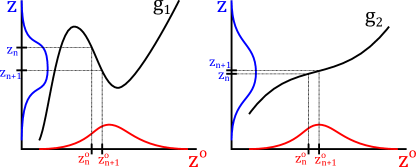
As is not changed by the representation, equality in (4) is approached by maximizing . That is, a good representation has high entropy (a wide distribution), but varies slowly with respect to changes in true state. If is constrained by the training loss (e.g. the KL divergence between and a unit normal distribution in VAEs [2]), minimizing approaches equality in (4).
can be approximated from the time-series properties of . Consider an initial and where , and define perturbations , . A first-order Taylor approximation gives . If , , then . Denote eigenvalues of of , then , , and
| (5) |
by the log sum inequality, where equality is attained if and only if , . Thus, when is constrained and is normal with zero mean with unit covariance, minimizing brings (4) closer to equality. Minimizing alone can be achieved by simply scaling the coordinates of – smoothness requires additional constraints on the representation to be useful.
Temporal Smoothness in Lagrangian systems
Denote temporal first difference , and second difference , which have both been used to measure smoothness [25, 3]. Taking dynamics of (1) where holonomic constraint has been eliminated, the explicit Euler approximation is
| (10) |
where is the sample time, , similarly . Considering (10) as a linear time-varying system (i.e. ignoring the nonlinearity from system matrices), if is compensated, initial velocity , and ,
| (11) |
where . When (i.e. random exploration), is a zero mean Gaussian. Furthermore, if eigenvalues (i.e. higher magnitude exploration noise in ‘slower’ degrees of freedom), position change has unit covariance.
If , and
| (12) |
Taking a first order approximation to the policy, . When is smooth; these terms will be small. In comparison with (11), reduces the bias in positions by a factor of at least . Additionally; the covariance of does not grow with , providing a more stationary distribution.
4 Validation
 |
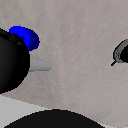 |
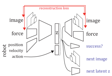
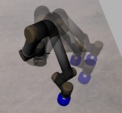
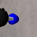
These experiments are conducted in a simulated peg-in-hole task where the hole position varies between iterations, a wrist camera provides 64x64 RGB images, and a 6-DOF force/torque sensor is mounted at the wrist. A dataset is collected with backwards exploration from the goal position as seen in Figure 3b, for 25 different hole positions (total 7500 samples). Several autoencoders are trained on this dataset, all of which are based on the classical VAE:
-
•
VAE, reconstruct image and force measurements [2]
-
•
success, add a success classifier [4]
-
•
predZ, add a loss for predicting the next latent state, based on current latent state and action
- •
-
•
smooth, which adds a smoothing loss [25].
The baseline autoencoder is implemented as seen in Figure 3a, where direct measurements from the robot of position, velocity, low-pass filtered force measurements, and torque input are processed by a modality-specific MLP, then fused with fully-connected layers to produce the distribution of . The latent , concatenated with torque input, is used to decode the original image and force. The convolutional stack for the images increases from 32 to 128 filters, filter size 4, stride 2/1, with ReLU activations. The force and proprioception encoders have one hidden layer of size 16, with a fusion encoder has a hidden layer of 64 units, fully-connected to mean and log standard deviation for . The decoder inverts this stack.
The success classifier contains 2 FC layers followed by softmax (success labels are identified by hand). The next image predictor has an additional FC layer before the deconvolution stack. The next latent predictor uses a hidden layer of size 64, ReLU activations for mean and log standard deviation of . The loss weights used for training are reconstruction , KL weight is normally, and with low KL encoders. The success weight is , smoothing weight , prediction of next weight and the prediction of next image weight . On the low KL smoothing, the smoothing weight was reduced to .
After encoder training, two model-free RL agents are trained: SAC [39] and DDPG [40], based on the code associated with [5]. The state given to the agent is the latent state (maximum likelihood, i.e. not a sample), augmented with the robot state. The agents are trained over 10 seeds each, with actor and critic architecture of two hidden layers of size 96 or 128, trained with Adam at learning rates or , replay buffer of 3e6, batch size of 256, and soft-update of . Noise tuning was used on SAC, and DDPG had constant exploration noise of magnitude the maximum input. RL agents are trained for 150k environment steps and evaluated for 20k steps. A video of the resulting performance is available at: https://youtu.be/adHXi58u9qw . A second dataset collects representation trajectories produced by a trained full-state SAC agent, to allow comparison between the representations on-policy in some of the following analysis.
4.1 Mutual information and performance
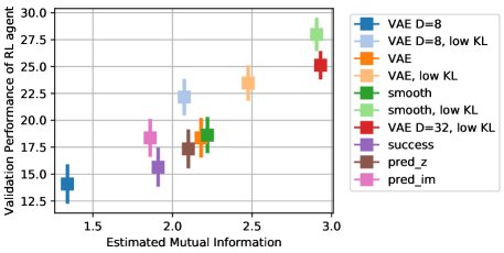
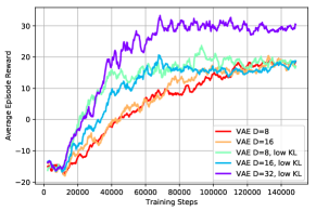
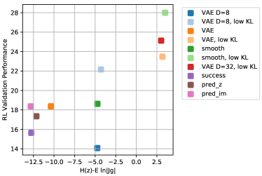
The mutual information between and is estimated with MINE [16], where the true state is the position/velocity of the robot, and the planar position of the hole. MINE is implemented with linear/ReLU layers with 64 hidden units, optimized with Adam at a learning rate of , batch size of 128. In Figure 4a, a strong correlation between estimated mutual information and RL performance can be seen over all tested encoders. The performance of the auxiliary training losses (predZ, predIM) is largely similar; there is not significant variation in performance or mutual information, while success slightly reduces both performance and mutual information in this example. The smoothness penalty increases the mutual information and performance in low KL case, but has more limited impact in the standard case.
Reducing the KL weight in the training loss significantly improves RL performance, as noted in existing work [5], and mutual information. This is also indicated by the -VAE analysis in [34], which suggests decreasing the KL weight increases the mutual information of the encoder. The tuning of the KL weight and the encoder architecture is substantially more important for performance in this task. As seen in Figure 4b, the encoders with a lower KL weight also train faster than their counterparts, while the dimension of the latent space does uniformly impact training speed.
4.2 Regression to True State
Regression from latent to the true state has also been employed as a validation in representation learning [8, 5], and proposed as a metric for representation quality [26, 27]. Here, the residual regression error is compared with RL performance and estimated mutual information in Figure 5a and 5b, respectively. The regression results use FC layers with ReLU activations, two hidden layers of 64 units, trained to minimize the L2 error on the combined random and on policy datasets, with 30% of the data held out for the validation, validation score reported in the figure.
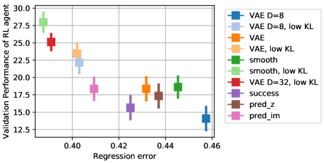
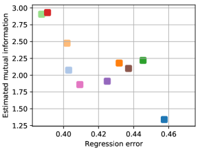
The L2 regression error also has a strong correlation with RL performance, suggesting that it also serves well as a metric for representation quality. Accordingly, a good correlation can be seen between the regression error and mutual information. Further experiments in other environments are required to make any general conclusions regarding the relative merits of regression error and mutual information as metrics.
4.3 Encoder Smoothness
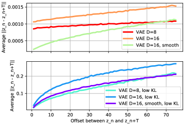
The assumptions and efficacy of the smoothing loss will be examined on the same dataset. First, the average distance between latent state at various time offset , , is shown in Figure 6a. Latent states which are temporally close are spatially closer for all encoders, but to varying degrees. The lower KL losses have latent representations which ‘grow apart’ more, and also had better RL performance. The VAE produces time-contrastive representations, even absent temporal information.
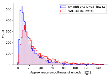
The smoothness of the encoding pipeline is then measured as , as shown in Figure 6b for the on-policy data (i.e. all representation trajectories are from the same true-state trajectory). The smoothed encoder has a lower average slope, changing less for small changes in true state.
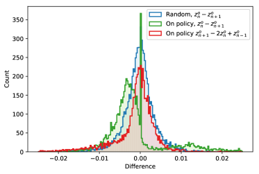
In (5), it was assumed that the first difference is normally distributed. The distribution of an element and the sum of the true state can be seen in Figure 7a, in both random and on-policy data. The first difference on the random agent (blue) is approximately normal, but the first difference on policy (green) is bimodal - the trained agent is moving towards the objective. However, the second difference on policy (red) removes this bias and is again approximately normal.
The objective of approaching equality in (4) can be investigated, estimating with the upper bound from (5) of , where is used and is the dimension of the representation. The entropy is estimated with a kNN estimator [41], allowing comparison between and performance, shown in Figure 7b. Representations which are high entropy and smooth (small ) approach equality in , where equality implies there is a function such that . The relationship seen in Figure 7b is not as strong as mutual information or regression, but suggest the objective in (5) is sensible.
5 Conclusion
Towards a connection between properties of a representation and its suitability for control, this paper proposed the objective of a unique representation; where each representation corresponds to a unique true state . This goal motivates two metrics: mutual information between and the temporal smoothness of . The proposed metrics show good predictive power for model-free reinforcement learning performance. While the true state is typically unknown, the first or second difference of the true state are normal, and zero-mean under certain conditions.
Further experimentation is needed to validate the initial results here on a wider range of robotics tasks, and on a wider range of representations (e.g. contrastive learning). However, the initial results can inform the tuning of hyperparameters and architecture of representation learning, which can greatly assist in hardware experiments with relatively expensive data collection.
References
- [1] Yoshua Bengio, Aaron Courville and Pascal Vincent “Representation Learning: A Review and New Perspectives” In IEEE transactions on pattern analysis and machine intelligence 35.8 IEEE, 2013, pp. 1798–1828
- [2] Diederik P. Kingma and Max Welling “Auto-Encoding Variational Bayes”, 2013 arXiv:1312.6114
- [3] Chelsea Finn et al. “Deep Spatial Autoencoders for Visuomotor Learning”, 2015 arXiv: http://arxiv.org/abs/1509.06113
- [4] Mel Vecerik et al. “A Practical Approach to Insertion with Variable Socket Position Using Deep Reinforcement Learning”, 2018 arXiv: http://arxiv.org/abs/1810.01531
- [5] Denis Yarats et al. “Improving Sample Efficiency in Model-Free Reinforcement Learning from Images”, 2020 arXiv: http://arxiv.org/abs/1910.01741
- [6] Manuel Watter, Jost Springenberg, Joschka Boedecker and Martin Riedmiller “Embed to Control: A Locally Linear Latent Dynamics Model for Control from Raw Images” In Advances in Neural Information Processing Systems 28 Curran Associates, Inc., 2015, pp. 2746–2754 URL: http://papers.nips.cc/paper/5964-embed-to-control-a-locally-linear-latent-dynamics-model-for-control-from-raw-images.pdf
- [7] Ershad Banijamali, Rui Shu, Hung Bui and Ali Ghodsi “Robust Locally-Linear Controllable Embedding” In International Conference on Artificial Intelligence and Statistics, 2018, pp. 1751–1759
- [8] Danijar Hafner et al. “Learning Latent Dynamics for Planning from Pixels” In International Conference on Machine Learning, 2019, pp. 2555–2565
- [9] Alex X. Lee, Anusha Nagabandi, Pieter Abbeel and Sergey Levine “Stochastic Latent Actor-Critic: Deep Reinforcement Learning with a Latent Variable Model”, 2020 arXiv: http://arxiv.org/abs/1907.00953
- [10] Pierre Sermanet et al. “Time-Contrastive Networks: Self-Supervised Learning from Video”, 2018 arXiv: http://arxiv.org/abs/1704.06888
- [11] Aravind Srinivas, Michael Laskin and Pieter Abbeel “CURL: Contrastive Unsupervised Representations for Reinforcement Learning”, 2020 arXiv: http://arxiv.org/abs/2004.04136
- [12] Francesco Locatello et al. “Challenging Common Assumptions in the Unsupervised Learning of Disentangled Representations”, 2018 arXiv:1811.12359
- [13] Ricky T.. Chen, Xuechen Li, Roger B Grosse and David K Duvenaud “Isolating Sources of Disentanglement in Variational Autoencoders” In Advances in Neural Information Processing Systems 31 Curran Associates, Inc., 2018, pp. 2610–2620 URL: http://papers.nips.cc/paper/7527-isolating-sources-of-disentanglement-in-variational-autoencoders.pdf
- [14] Anthony Bloch et al. “Nonholonomic Mechanics and Control” Springer, 2003
- [15] Mary Phuong et al. “The Mutual Autoencoder: Controlling Information in Latent Code Representations”, 2018
- [16] Mohamed Ishmael Belghazi et al. “Mine: Mutual Information Neural Estimation”, 2018 arXiv:1801.04062
- [17] S. Lange, M. Riedmiller and A. Voigtländer “Autonomous Reinforcement Learning on Raw Visual Input Data in a Real World Application” In The 2012 International Joint Conference on Neural Networks (IJCNN), 2012, pp. 1–8 DOI: 10.1109/IJCNN.2012.6252823
- [18] David Ha and Jürgen Schmidhuber “World Models”, 2018 arXiv:1803.10122
- [19] Marvin Zhang et al. “SOLAR: Deep Structured Representations for Model-Based Reinforcement Learning”, 2018 arXiv: http://arxiv.org/abs/1808.09105
- [20] Debidatta Dwibedi, Jonathan Tompson, Corey Lynch and Pierre Sermanet “Self-Supervised Representation Learning for Continuous Control”, 2018
- [21] Michelle A. Lee et al. “Making Sense of Vision and Touch: Learning Multimodal Representations for Contact-Rich Tasks” In IEEE Transactions on Robotics 36.3, 2020, pp. 582–596 DOI: 10.1109/TRO.2019.2959445
- [22] Joshua C. Triyonoputro, Weiwei Wan and Kensuke Harada “Quickly Inserting Pegs into Uncertain Holes Using Multi-View Images and Deep Network Trained on Synthetic Data”, 2019 arXiv: http://arxiv.org/abs/1902.09157
- [23] Jianlan Luo et al. “Reinforcement Learning on Variable Impedance Controller for High-Precision Robotic Assembly”, 2019 arXiv:1903.01066
- [24] Laurenz Wiskott and Terrence J. Sejnowski “Slow Feature Analysis: Unsupervised Learning of Invariances” In Neural Computation 14.4, 2002, pp. 715–770 DOI: 10.1162/089976602317318938
- [25] Rico Jonschkowski, Roland Hafner, Jonathan Scholz and Martin Riedmiller “PVEs: Position-Velocity Encoders for Unsupervised Learning of Structured State Representations”, 2017 arXiv: http://arxiv.org/abs/1705.09805
- [26] Antonin Raffin et al. “S-RL Toolbox: Environments, Datasets and Evaluation Metrics for State Representation Learning”, 2018 arXiv: http://arxiv.org/abs/1809.09369
- [27] Rika Antonova, Sam Devlin, Katja Hofmann and Danica Kragic “Benchmarking Unsupervised Representation Learning for Continuous Control”, 2020 URL: https://openreview.net/forum?id=UKqIsgNeah7
- [28] Karl Johan “ AAström and Richard M. Murray “Feedback Systems: An Introduction for Scientists and Engineers” Princeton university press, 2010
- [29] Anthony M. Bloch, Mahmut Reyhanoglu and N. McClamroch “Control and Stabilization of Nonholonomic Dynamic Systems” In IEEE Transactions on Automatic control 37.11, 1992, pp. 1746–1757
- [30] Thomas M. Cover “Elements of Information Theory” John Wiley & Sons, 1999
- [31] David Barber and Felix V. Agakov “The IM Algorithm: A Variational Approach to Information Maximization” In Advances in Neural Information Processing Systems, 2003, pp. None
- [32] Ben Poole et al. “On Variational Bounds of Mutual Information”, 2019 arXiv:1905.06922
- [33] Irina Higgins et al. “Beta-VAE: Learning Basic Visual Concepts with a Constrained Variational Framework.” In Iclr 2.5, 2017, pp. 6
- [34] Alexander A. Alemi et al. “Fixing a Broken ELBO”, 2017 arXiv:1711.00464
- [35] Mary Phuong et al. “The Mutual Autoencoder: Controlling Information in Latent Code Representations”, 2018
- [36] Shengjia Zhao, Jiaming Song and Stefano Ermon “InfoVAE: Information Maximizing Variational Autoencoders”, 2018 arXiv: http://arxiv.org/abs/1706.02262
- [37] Athanasios Papoulis and S. Pillai “Probability, Random Variables, and Stochastic Processes” Tata McGraw-Hill Education, 2002
- [38] Herke Hoof et al. “Stable Reinforcement Learning with Autoencoders for Tactile and Visual Data” In 2016 IEEE/RSJ International Conference on Intelligent Robots and Systems (IROS) Daejeon, South Korea: IEEE, 2016, pp. 3928–3934 DOI: 10.1109/IROS.2016.7759578
- [39] Tuomas Haarnoja, Aurick Zhou, Pieter Abbeel and Sergey Levine “Soft Actor-Critic: Off-Policy Maximum Entropy Deep Reinforcement Learning with a Stochastic Actor”, 2018 arXiv:1801.01290
- [40] Timothy P. Lillicrap et al. “Continuous Control with Deep Reinforcement Learning”, 2015 arXiv:1509.02971
- [41] Alexander Kraskov, Harald Stögbauer and Peter Grassberger “Estimating Mutual Information” In Physical review E 69.6 APS, 2004, pp. 066138
Appendix A Appendix
A.1 Estimating Mutual Information, Smoothness, Regression
MINE [16] is used for the mutual information estimates reported in the text, based on implementation [kim]. These were compared with k-nearest neighbor approaches [41], where many of the same trends emerge but the KNN methods struggled with low-entropy random variables. MINE provided high-variance estimates, ameliorated with large batch sizes, a lower learning rate, and a small moving average constant (0.001) for the unbiased estimator. The network consist of linear/ReLU layers with 64 hidden units, Adam is used for optimization, with a learning rate of , batch size of 128.
The regression results use FC layers with ReLU activations, two hidden layers of 64 units, trained to minimize the L2 error on the combined random and on policy datasets, with 30% of the data held out for the validation, validation score reported in the figure.
A.2 Encoder
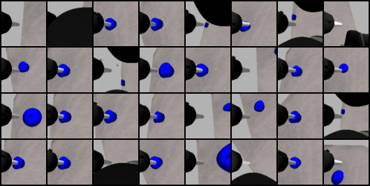
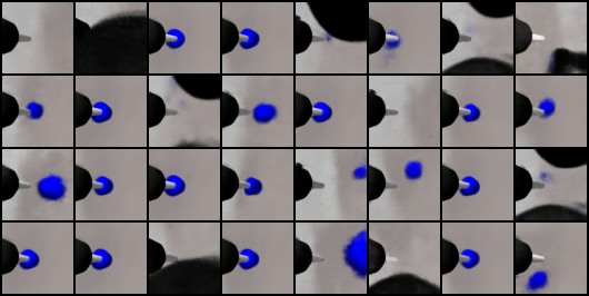
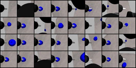
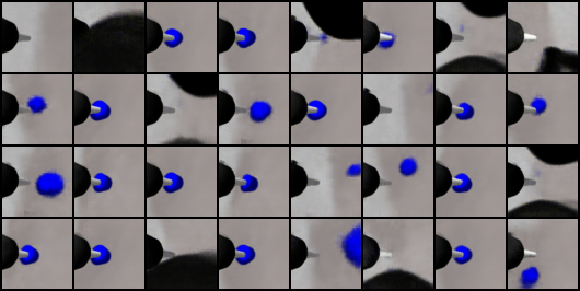
The convolutional stack for the images increases from 32 to 128 filters, filter size 4, stride 2/1, with ReLU activations. The force and proprioception encoders have one hidden layer of size 16, with a fusion encoder has a hidden layer of 64 units, fully-connected to mean and log standard deviation for . The decoder inverts this stack. Sample reconstructions can be seen in Figure 8.
The success classifier contains 2 FC layers followed by softmax (success labels are identified by hand). The next image predictor has an additional FC layer before the deconvolution stack. The next latent predictor uses a hidden layer of size 64, ReLU activations for mean and log standard deviation of .
The loss weights used for training are reconstruction , KL weight is normally, and with low KL encoders. The success weight is , smoothing weight , prediction of next weight and the prediction of next image weight . On the low KL smoothing, the smoothing weight was reduced to .
A.3 RL Agent
A standard implementation of SAC is used [5] and ablated to implement the DDPG agent. Actor and critic architecture have two hidden layers of size 96 or 128 (varied to average performance). The agents were trained with learning rates or , replay buffer of 3e6, batch size of 256, and soft-update of . Noise tuning was used on SAC, and DDPG had constant exploration noise of magnitude the maximum input. The agents were trained from 10 different random seeds each.
The simulation is done with the ODE dynamics engine [smith2005], under contact constraint settings of , and , and maximum step size of . The reward function largely follows that of [lee2018a].
A.4 Derivation of bound on
Recall that where are the eigenvalues of . If ,
Applying the log sum inequality, where for positive constants , , , :
letting , ,
By substitution,