Learning-based State Reconstruction
for a Scalar Hyperbolic PDE under noisy Lagrangian Sensing
Abstract
The state reconstruction problem of a heterogeneous dynamic system under sporadic measurements is considered. This system consists of a conversation flow together with a multi-agent network modeling particles within the flow. We propose a partial-state reconstruction algorithm using physics-informed learning based on local measurements obtained from these agents. Traffic density reconstruction is used as an example to illustrate the results and it is shown that the approach provides an efficient noise rejection.
keywords:
state reconstruction, hyperbolic PDE, Lagrangian sensing, noise rejection, physics-informed deep learning1 Introduction
Traffic jams are a source of green gas and time-consumption (Ferrara et al., 2018). One solution to lighten the effect of congestion is to control the flow of vehicles. There exist a large variety of control strategies using variable speed limits (Delle Monache et al., 2017), ramp control (Zhang et al., 2019) or autonomous vehicles (Piacentini et al., 2018; Wu et al., 2017). These laws require knowledge of road density everywhere. There comes the need for an efficient state reconstruction algorithm using measurements from fixed sensors but also capable of dealing with GPS measurements (Amin and al., 2008) and Probe Vehicles (PVs) sensing (Herrera and Bayen, 2010).
This is challenging from a theoretical point of view since such a system is modeled by a cascaded partial differential equation with a multi-agents network (C-PDE-MA) such as the one derived by meBorsche et al. (2012). There exist several kinds of algorithms to estimate the density and one can refer to the survey by Seo et al. (2017) for an overview. For fixed sensors, one can investigate the use of backstepping observers (Smyshlyaev and Krstic, 2005). However, these cannot deal effectively with nonlinearities and one has to approximate the system dynamic depending on its regime (Yu et al., 2019). Using PVs, there exist some open-loop state reconstruction algorithms proposed for instance by Delle Monache et al. (2019); Barreau et al. (2020); Čičić et al. (2020). They are copying the system and matching the boundary conditions, consequently, they are not robust to model mismatch or noise. Another recent field of research is to use machine learning tools to estimate the density (Matei et al., 2019; Huang and Agarwal, 2020; Liu et al., 2021), no matter the origin of the measurement. They are then more flexible and they lead to a good reconstruction providing substantial computer resources.
This paper goes in that latter direction and extends the preliminary observations made in Liu et al. (2021). One contribution of this article is to define a partial-state reconstruction (P-SR) expressed as the solution to an optimization problem. We show that a neural network is capable of solving the noisy state reconstruction problem asymptotically and we explain how two neural networks with a dense architecture are well-suited to that problem. We also propose a training procedure that is robust with a moderate computational burden.
The outline of the paper is as follows. In Section 2, we describe the model C-PDE-MA and give some fundamental properties about the existence and regularity of solutions. We end this section by giving a general definition of state reconstruction. Similarly to what is proposed by Ostrometzky et al. (2019), Section 4 is dedicated to the neural network solution with a particular focus on the numerical implementation. Finally, we consider the traffic state reconstruction problem, and simulations show a good reconstruction accuracy, even in the noisy case. The conclusion enlarges the scope of the article by providing some perspectives.
Notation: We define , and as the spaces of locally integrable functions, bounded functions and continuous functions of class from to , respectively. A function in is piecewise-. Let be a function defined in a neighborhood of a point , we define as . For a function defined in a neighborhood of with , we write if .
2 Problem Statement
This section introduces some fundamental notions about the PDE model, the ODE model, and their coupling. It is followed by the problem considered in this paper. Theoretical questions regarding the existence and regularity of solutions to these models are also briefly discussed.
2.1 PDE model
To define our problem, we will use the notation introduced by Bastin and Coron (2016). We are interested in the following scalar hyperbolic and quasi-linear PDE for :
| (1) |
with initial condition is piece-wise . In physical systems, usually refers to the normalized density. Equation (1) is then the macroscopic expression of the conservation of mass.
We assume that
-
1.
is of class ,
-
2.
The flux function is concave,
-
3.
, where is the free flow speed.
Proposition 1
There exist weak solutions to this system with the following regularity:
| (2) |
The regularity result comes from a direct application of Theorems 6.2.2 and 11.3.10 by Dafermos (2010). The fact that is a consequence of the generalized characteristic methodology (Protter and Weinberger, 2012, Chap. 4). Considering the Lax-E entropy condition guarantees that the solution is unique (Dafermos, 2010, Theorem 14.10.2). Note that is concave, hence, the entropy condition turns out to be:
| (3) |
2.2 Agents model
Consider a network of agents, located at , such that . These agents are particles within a flow of local density defined in (1). In other words, can be seen as a probability distribution and the agents are a subset of a given realization.
We assume first that the speed of agent depends only on the density at its location and that is a decreasing function of the density. Since the density might be discontinuous, we consider that the speed is the infimum in any neighborhood around its position. Because of the entropy condition (3), the velocity function writes as:
The agent’s dynamic is then modeled by the following ordinary differential equation (ODE):
| (4) |
Under the entropy condition (3), one can show that the agents stay ordered in space, meaning that for any . Since the number of particles between agents and is and a particle cannot overtake another one, the quantity remains constant and
where . The previous expression must hold for any yielding:
| (5) |
Because is concave and , we get that is indeed a decreasing function of the density.
Proposition 2
There exists a unique absolutely continuous solution of (4) defined for .
Proof 2.1.
From the definition of , we get that . The proposition results from the application of Carathéodory theorem (Coddington and Levinson, 1955, Theorem 1.1, Chap 2).
2.3 C-PDE-MA model
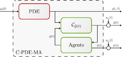
In this paper, the network of agents is capable of sensing the PDE state at their locations. The C-PDE-MA model is illustrated in Figure 1. It is represented by a coupling between the PDE model (1) and the ODE model (4) for and :
| (6) |
where are measurement noises, is the element-wise function defined in (5), and . The operator represents the way the agents are sensing, which ends up being:
2.4 Problem formulation
We are interested in this paper in the reconstruction of the PDE state as expressed by the block diagram in Figure 1. Before stating the problem, some definitions are given below.
Definition 2.2.
Let , be a semi-normed vector space and a subset of . The partial-reconstructed set in of is defined as the set:
| (7) |
We say that a signal is a partial-state reconstruction (P-SR) if .
Remark 2.3.
Note that this definition encapsulates the following cases:
-
•
If and then almost everywhere and this is the definition of an asymptotic state reconstruction.
-
•
If is a vector space and , then the P-SR is the orthogonal projection of on .
The state reconstruction problem implies to choose three entities: the space referring to the spatial domain of ; a subset where we seek and the semi-norm on . We will construct these three entities in the sequel.
We are working on a time window (we gather measurements during this time period). For the space interval, we are interested in the reconstruction between the first and the last agents. As noted in (2), we get . In the case without noise and if we assume that the model (6) is known, we get that where:
with . Note that is generally not a vector space. As noted by Klibanov (2006); Gosse and Zuazua (2017), even if , is usually not a singleton since there is no information on the initial condition. However, there always exists at least one weak solution to (1) so is not empty.
Adding bias on the measurements implies that does not belong to . Consequently, it is better to use Definition 2.2 with and for :
| (8) |
It is difficult to solve the optimization problem (7) since the solution to (1) is usually not smooth (Bastin and Coron, 2016). One way to overcome this issue is to consider a slightly different partial differential equation:
| (9) |
where . This equation has many interesting properties and in particular, the solutions are smoother than in (1). Using (Amann, 1993, Theorem 14.6) with piece-wise boundary conditions, then
| (10) |
Moreover, the vanishing viscosity method applied to this problem (Coclite and Garavello, 2013, Lemma 4.2) shows that the solution to (9) converges in a weak sense to the entropic solution to (1) as goes to zero. The set becomes then:
| (11) |
Using the previous definitions, we can define the partial-reconstructed set .
Since the set contains an equality constraint, it might be difficult to solve the optimization problem (7) with (8)-(11). Using the Lagrange multiplier , we propose the following relaxation:
| (12) |
where . It follows from the previous discussion that and, in a weak-sense . An element of is a P-SR of solution to (6) in for the semi-norm (8). The objective rewrites then as follows.
Rephrased objective: Find a signal with the smallest .
To the best of the author knowledge, the P-SR solution to an hyperbolic PDE with noisy measurements coming from a network of agents has never been considered in the literature. We propose to solve this using machine learning as explained in the following section.
3 Learning-based State Reconstruction
This section is divided into two subsections. In the first one, we derive a P-SR problem associated to (6) without noise. In the second one, the same is discussed with addition of noisy measurements.
3.1 Neural network solution to the P-SR problem without noise
A neural network of neurons designed for a regression problem is the mapping , where and are the bias and the weight tensors respectively. is the element-wise activation function. A densely connected deep-neural network is a neural network with layers, meaning that . This neural network is trained on the data-set , meaning that the weights and biases are found as the arguments that locally minimizes a loss function . For regression problems, the loss function is usually chosen to be where is the number of measurements. This is the Mean-Square Error (MSE) between the observed and estimated outputs. Note that this loss function is a discretization of the -norm of the error on the whole space .
We cannot measure points all over the domain but only on the image of the operator . For uniformly distributed in , uniformly distributed in and , an equivalent discretization of the cost function in (12) is:
| (13) |
is divided into three parts:
-
1.
the first term is the traditional MSE over the measurements.
-
2.
the second term (often called the physics MSE) does not rely on measurements but only depends on the weights and biases of the neural network, it is derived using automatic differentiation (Baydin et al., 2017) based on the dynamic of the system. As stressed in Raissi et al. (2019),it can be seen as a regularization agent, preventing over-fitting by disregarding non physical solutions and reducing the impact of the noise by enforcing the model. The choice of the weight depends then on the confidence we have in the model and the sparsity of the dataset.
- 3.
The second term of the previous objective function was introduced by Lagaris et al. (1998); Psichogios and Ungar (1992) where the authors used a neural network to provide a solution to a differential equation. It has been investigated more recently in Raissi et al. (2019) under the name ”Physics-informed deep learning” where it has been extended to robust parameter identification.
Using a backpropagation algorithm, we train the neural network by locally solving the following optimization problem:
| (14) |
Using a neural network to solve this problem is reasonable since, as shown in Sirignano and Spiliopoulos (2018), it has a convergence property recalled below.
Theorem 1
In the case , the following holds:
3.2 Neural network solution to the P-SR problem with noise
First, assume that is a realization of a Gaussian distribution with mean and standard deviation . The current optimization problem (14) implies the minimization of a MSE, consequently, the variance of the noise on the agents’ trajectories is minimized. The second part of the cost function enforces the signal to be a solution to the noiseless model keeping a low variance as well. Such an implementation performs well and rejects the unbiased noise (Raissi et al., 2019).
In the biased case, if is large enough, we get . Consequently, small and yield and is not a local minimizer. One solution to this issue is to consider instead the loss function where .
To deal with the noise , the neural network architecture has to be modified. In that case, one need to propose a similar architecture with some physics cost on , leading to the diagram in Figure 2. There are then two neural networks that are trained simultaneously. is the same as in the previous part and the second one, , estimates . Naturally, the loss function is:
where is defined in (13), , and .
Remark 3.1.
The physics cost related to the trajectories of the agents is adding some artificial boundary data. Consequently, the measurements can be sparser for a similar trajectory estimation.

3.3 Numerical implementation
3.3.1 Network architecture
It is well-known that some solutions of (1) are discontinuous while solutions of (9) are usually not. Nevertheless, they may have fast variations. The neural network must handle both shock and rarefaction waves while represents an absolutely continuous function.
takes one input (the time ) and has outputs (the positions of the agents). Since the solution is absolutely continuous (it is piece-wise ), the best is to combine some and activation functions. To keep a simple structure, one can then consider two dense neural networks with different activation functions such as and . They are summed and weighed at the end to give the final output. There are hidden layers, each with neurons for each sub-network.
For , the architecture is more complex. Since we are considering a viscous PDE, the solutions are continuous and using the as an activation function seems a good choice for several reasons:
-
1.
A dense neural network with activation functions can deal with almost-shock waves since where is the trajectory of a shock wave. If is chosen very large, then there is a very steep slope along the curve .
-
2.
It can deal with rarefaction waves as well since in this case the solution is (Evans, 1998, Section 11.2) which is continuous since is and .
Consequently, the number of nodes can be related to the number of waves in the solution. On the contrary, the number of layers deals with the inference between these waves. In conclusion, the number of nodes is related to the length-space while the number of layers reflects the time-window. Choromanska et al. (2015) showed that having a neural network with many variables usually leads to better convergence. As said previously, the neural network should not overfit the data because of the regularization agent so we can consider a large network with layers made up of neurons each.
3.3.2 Training procedure
First of all, since the space and time intervals are not of the same order of magnitude, it is better to standardize the dataset before training. Indeed, that leads to a faster convergence of the optimization procedure to a more optimal solution (Goodfellow et al., 2016).
Similarly to what was done in Raissi et al. (2019); Lagaris et al. (1998); Sirignano and Spiliopoulos (2018), the best solver for this problem seems to be the BFGS algorithm (Nocedal and Wright, 2006, Chap 6). Nevertheless, it is quite slow so one can consider speeding it up with a pre-training using Adam (Kingma and Ba, 2015). Another issue comes with the choice of the different . It appears that the effect of this choice decreases when we split the training into several steps, leading to the following procedure:
-
1.
Let and , . We then estimate precisely the trajectories of the agents and we modify the value of the density along these curves. We train using the BFGS algorithm with low requirements such that the convergence is rapidly obtained.
-
2.
Then, we train the value of the density without modifying the trajectories. For that, we fix the neural network and we use first Adam and then BFGS with , , and . This step takes more time and fixes the values of the density at its boundaries while starting to enforce the physics of the PDE inside the domain.
-
3.
Finally, we optimize using BFGS only and , , , and . We focus on this step on the noise reduction and we minimize the coupled system proposed in Figure 2. Since the trajectories are close to their optimal values, this step changes mostly the values of the density inside the domain, trying to keep a low value of .
This procedure seems, in general, to be a good starting point for such a problem since it follows the iterative procedure described in Bertsekas (2014). The weights values have to be designed in each case and the one used here leads to the lowest computed generalization error in our case.
4 Traffic flow theory and simulation results
4.1 Traffic flow theory
The simplest model for traffic flow on a highway is given by the continuity equation, which is nothing more than the conservation of mass (Evans, 1998, Chapter 11). This model has been derived by Lighthill and Whitham (1955); Richards (1956) and it results in the so-called LWR model:
| (15) |
where is the normalized density of cars. It can be represented as the probability distribution of a car at a given position at time . stands for the equilibrium velocity of a car depending on the density around. The LWR model assumes, similarly to Greenshields et al. (1935), that , where is the free flow speed. With this choice, (15) transforms into the following scalar hyperbolic PDE for :
| (16) |
In the context of traffic flow, we are considering that there are some vehicles – called Probe Vehicles (PV) – capable of sensing the density around them using the distances to their neighbors, cameras (Chellappa et al., 2004; Kang and Kum, 2020) or radar sensors (Sun et al., 2006). The state reconstruction problem without noise is solved in finite-time by Delle Monache et al. (2019); Barreau et al. (2020) for instance. The results in our case are shown in the following subsection. A full study on this example is conducted in Liu et al. (2021).
4.2 Simulation results
We are studying here the P-SR problem of (16) using probe vehicles. The real density is obtained from a Godunov scheme (LeVeque, 1992) with random initial and boundary conditions. One can see in Figure 3 that shocks and rarefaction waves are making the reconstruction difficult. We did the reconstruction in two cases with a neural network coded using Tensorflow 1.15 (Abadi and al., 2015; Barreau and Liu, 2020). The first scenario considers the system without noise; the result is displayed in Figure 4. The second case contemplates as an unbiased Gaussian noise with a standard deviation of and as a Brownian motion generated from a normal distribution with zero mean and a variance (see Figure 4). P-SR are done using a naive BFGS Raissi et al. (2019); Sirignano and Spiliopoulos (2018) and others using the training procedure described earlier. The computations are done on a Intel Core i5-8365 CPU @ 1.60GHz and 16 GB of RAM computer. The computation time and the normalized error are displayed in Figure LABEL:fig:stats.
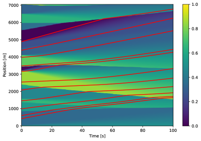
fig:rho_example
\subfigure[Scenario without noise]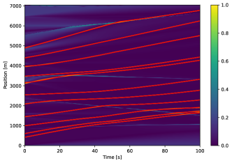 \subfigure[Scenario with noise]
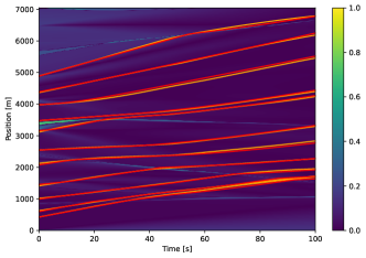
fig:stats
\subfigure[Computation time in seconds]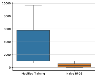 \subfigure[Normalized generalization error]
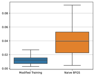
One can see in Figure 4 that the reconstruction in the first case is almost perfect. There are some discrepancies for small-time because of the effect of the unknown initial condition. But, after a while, the reconstruction error is close to zero between the PV except on the shock trajectories where the neural network is unable of reproducing the steep variation. In the second case (see Figure 4), the error is larger. The PV trajectories are not as sharp as in the first case because of the noise correction. Nevertheless, the P-SR is very close to the one obtained previously, showing that the proposed solution is indeed capable of reducing the noise in the measurements. The modified training has a larger computation time ( times larger in average) but a smaller and more consistent generalization error ( times smaller in average with a standard deviation is times smaller). That means the modified training procedure is indeed more accurate and robust to the neural network initialization at the price of a much larger computation time.
5 Conclusion & Perspectives
In this paper, we proposed the partial-state reconstruction problem of a hyperbolic equation using only Lagrangian measurements and we applied it to the special example of traffic flow estimation. To that extend, we used physics-informed deep learning to counterbalance the small number of measurements and increase the robustness. The simulations showed that noise was indeed rejected.
This is preliminary work and we propose many perspectives. First of all, the neural network can be improved by considering a more specific architecture (Hochreiter and Schmidhuber, 1997). One can also look into the direction of a decentralized reconstruction algorithm, that would effectively reduce the computational burden while increasing the sensitivity to noise. The roles of the have not been explored in the paper, however, it appears that the speed of convergence highly depends on these values. A theoretical study on the role of these multipliers should be done to get a better understanding of the optimization process. Finally, one can also consider second-order models which are more adapted to traffic flow (Aw and Rascle, 1995; Zhang, 2002).
The research leading to these results is partially funded by the KAUST Office of Sponsored Research under Award No. OSR-2019-CRG8-4033, the Swedish Foundation for Strategic Research, the Swedish Research Council and Knut and Alice Wallenberg Foundation.
Appendix A Proof of Theorem 1
First of all, note that for a number of physical and measurement points sufficiently large, with is arbitrary close to defined as:
We will then consider the minimization of instead of the minimization of in the sequel.
We follow a proof similar to the one of Theorem 7.1 by Sirignano and Spiliopoulos (2018). Let us first denote by for the solutions of the following systems for :
| (17) |
We want to show that the minimum value of when is zero. Since , we then get
The last inequalities are obtained using Young inequality. Since lies in a compact set and , there exists such that . That yields:
The regularity of expressed by (10) implies that Theorem 3 by Hornik (1991) holds. That yields for any , there exists sufficiently large such that
That leads to
Because of the regularity properties of (see (10)) and , we indeed get that . That means in particular that almost everywhere and .
References
- Abadi and al. (2015) M. Abadi and al. TensorFlow: Large-scale machine learning on heterogeneous systems, 2015. URL https://www.tensorflow.org/. Software available from tensorflow.org.
- Amann (1993) H. Amann. Nonhomogeneous linear and quasilinear elliptic and parabolic boundary value problems. In Function spaces, differential operators and nonlinear analysis, pages 9–126. Springer, 1993.
- Amin and al. (2008) S. Amin and al. Mobile century using GPS mobile phones as traffic sensors: A field experiment. In 15th World Congress on Intelligent Transportation Systems, 2008.
- Aw and Rascle (1995) A. Aw and M Rascle. Resurrection of ”second order” models of traffic flow. SIAM J. Appl. Math., 60(3):916–938, 1995.
- Barreau and Liu (2020) M. Barreau and J. Liu. Learning-based traffic reconstruction using probe vehicles. https://github.com/mBarreau/TrafficReconstructionDL, 2020.
- Barreau et al. (2020) M. Barreau, A. Selivanov, and K. H. Johansson. Dynamic traffic reconstruction using probe vehicles. In Conference on Decision and Control (CDC), Jeju Island, Republic of Korea, 2020.
- Bastin and Coron (2016) G. Bastin and J.-M. Coron. Stability and boundary stabilization of 1-d hyperbolic systems, volume 88. Springer, 2016.
- Baydin et al. (2017) A. G. Baydin, B. A. Pearlmutter, A. A. Radul, and J. M. Siskind. Automatic differentiation in machine learning: a survey. The Journal of Machine Learning Research, 18(1):5595–5637, 2017.
- Bertsekas (2014) Dimitri P Bertsekas. Constrained optimization and Lagrange multiplier methods. Academic press, 2014.
- Borsche et al. (2012) R. Borsche, R. M. Colombo, and M. Garavello. Mixed systems: Odes–balance laws. Journal of Differential equations, 252(3):2311–2338, 2012.
- Chellappa et al. (2004) R. Chellappa, G. Qian, and Q. Zheng. Vehicle detection and tracking using acoustic and video sensors. In 2004 IEEE International Conference on Acoustics, Speech, and Signal Processing, volume 3, pages iii–793. IEEE, 2004.
- Choromanska et al. (2015) A. Choromanska, M. Henaff, M. Mathieu, G. B. Arous, and Y. LeCun. The loss surfaces of multilayer networks. In Artificial intelligence and statistics, pages 192–204, 2015.
- Coclite and Garavello (2013) G. M. Coclite and M. Garavello. Vanishing viscosity for mixed systems with moving boundaries. Journal of Functional Analysis, 264(7):1664–1710, 2013.
- Coddington and Levinson (1955) E. A. Coddington and N. Levinson. Theory of ordinary differential equations. Tata McGraw-Hill Education, 1955.
- Dafermos (2010) C. M. Dafermos. Hyperbolic Conservation Laws in Continuum Physics; 3rd ed. Grundlehren der mathematischen Wissenschaften. Springer, Dordrecht, 2010. 10.1007/978-3-642-04048-1.
- Delle Monache et al. (2017) M. L. Delle Monache, B. Piccoli, and F. Rossi. Traffic regulation via controlled speed limit. SIAM Journal on Control and Optimization, 55(5):2936–2958, 2017.
- Delle Monache et al. (2019) M. L. Delle Monache, T. Liard, B. Piccoli, R. Stern, and D. Work. Traffic reconstruction using autonomous vehicles. SIAM Journal on Applied Mathematics, 79(5):1748–1767, 2019.
- Evans (1998) L. C. Evans. Partial Differential Equations. Graduate studies in mathematics. American Mathematical Society, 1998. ISBN 9780821807729.
- Ferrara et al. (2018) A. Ferrara, S. Sacone, and S. Siri. Freeway Traffic Modelling and Control. Springer Nature, 2018.
- Goodfellow et al. (2016) I. Goodfellow, Y. Bengio, and A. Courville. Deep Learning. MIT Press, 2016.
- Gosse and Zuazua (2017) L. Gosse and E. Zuazua. Filtered gradient algorithms for inverse design problems of one-dimensional burgers equation. In Innovative algorithms and analysis, pages 197–227. Springer, 2017.
- Greenshields et al. (1935) B. D. Greenshields, J. R. Bibbins, W. S. Channing, and H. H. Miller. A study of traffic capacity. In Highway research board proceedings, volume 14. National Research Council (USA), Highway Research Board, 1935.
- Herrera and Bayen (2010) J. C. Herrera and A. M. Bayen. Incorporation of lagrangian measurements in freeway traffic state estimation. Transportation Research Part B: Methodological, 44(4):460–481, 2010.
- Hochreiter and Schmidhuber (1997) S. Hochreiter and J. Schmidhuber. Long short-term memory. Neural computation, 9(8):1735–1780, 1997.
- Hornik (1991) K. Hornik. Approximation capabilities of multilayer feedforward networks. Neural networks, 4(2):251–257, 1991.
- Huang and Agarwal (2020) J. Huang and S. Agarwal. Physics informed deep learning for traffic state estimation. In 2020 23rd International Conference on Intelligent Transportation Systems (ITSC). IEEE, 2020.
- Kang and Kum (2020) D. Kang and D. Kum. Camera and radar sensor fusion for robust vehicle localization via vehicle part localization. IEEE Access, 8:75223–75236, 2020.
- Kingma and Ba (2015) D. P. Kingma and J. Ba. Adam: A method for stochastic optimization. In 3rd International Conference for Learning Representations, 2015.
- Klibanov (2006) M. V. Klibanov. Estimates of initial conditions of parabolic equations and inequalities via lateral Cauchy data. Inverse problems, 22(2):495, 2006.
- Lagaris et al. (1998) I. E. Lagaris, A. Likas, and D. I. Fotiadis. Artificial neural networks for solving ordinary and partial differential equations. IEEE transactions on neural networks, 9(5):987–1000, 1998.
- LeVeque (1992) R. J. LeVeque. Numerical methods for conservation laws, volume 3. Springer, 1992.
- Lighthill and Whitham (1955) M. J. Lighthill and G. B. Whitham. On kinematic waves II. a theory of traffic flow on long crowded roads. Proceedings of the Royal Society of London. Series A. Mathematical and Physical Sciences, 229(1178):317–345, 1955.
- Liu et al. (2021) J. Liu, M. Barreau, M. Čičić, and K. H. Johansson. Learning-based traffic state reconstruction using probe vehicles. In 16th IFAC Symposium on Control in Transportation Systems (CTS), 2021.
- Matei et al. (2019) I. Matei, C. Mavridis, J. S. Baras, and M. Zhenirovskyy. Inferring particle interaction physical models and their dynamical properties. In 2019 IEEE 58th Conference on Decision and Control (CDC), pages 4615–4621. IEEE, 2019.
- Nocedal and Wright (2006) J. Nocedal and S. Wright. Numerical optimization. Springer Science & Business Media, 2006.
- Ostrometzky et al. (2019) J. Ostrometzky, K. Berestizshevsky, A. Bernstein, and G. Zussman. Physics-informed deep neural network method for limited observability state estimation. arXiv preprint arXiv:1910.06401, 2019.
- Piacentini et al. (2018) G. Piacentini, P. Goatin, and A. Ferrara. Traffic control via moving bottleneck of coordinated vehicles. IFAC-PapersOnLine, 51(9):13 – 18, 2018. ISSN 2405-8963. 15th IFAC Symposium on Control in Transportation Systems CTS 2018.
- Protter and Weinberger (2012) M. H. Protter and H. F. Weinberger. Maximum principles in differential equations. Springer Science & Business Media, 2012.
- Psichogios and Ungar (1992) D. C. Psichogios and L. H. Ungar. A hybrid neural network-first principles approach to process modeling. AIChE Journal, 38(10):1499–1511, 1992.
- Raissi et al. (2019) M. Raissi, P. Perdikaris, and G. E. Karniadakis. Physics-informed neural networks: A deep learning framework for solving forward and inverse problems involving nonlinear partial differential equations. Journal of Computational Physics, 378:686–707, 2019.
- Richards (1956) P. I. Richards. Shock waves on the highway. Operations research, 4(1):42–51, 1956.
- Seo et al. (2017) T. Seo, A. M. Bayen, T. Kusakabe, and Y. Asakura. Traffic state estimation on highway: A comprehensive survey. Annual Reviews in Control, 43:128–151, 2017.
- Sirignano and Spiliopoulos (2018) J. Sirignano and K. Spiliopoulos. DGM: A deep learning algorithm for solving partial differential equations. Journal of computational physics, 375:1339–1364, 2018.
- Smyshlyaev and Krstic (2005) A. Smyshlyaev and M. Krstic. Backstepping observers for a class of parabolic PDEs. Systems & Control Letters, 54(7):613–625, 2005.
- Sun et al. (2006) Z. Sun, G. Bebis, and R. Miller. On-road vehicle detection: a review. IEEE Transactions on Pattern Analysis and Machine Intelligence, 28(5):694–711, 2006.
- Čičić et al. (2020) M. Čičić, M. Barreau, and K. H. Johansson. Numerical investigation of traffic state reconstruction and control using connected automated vehicles. In 23rd International Conference on Intelligent Transportation Systems (ITSC), 2020.
- Wu et al. (2017) C. Wu, A. Kreidieh, K. Parvate, E. Vinitsky, and A. M. Bayen. Flow: Architecture and benchmarking for reinforcement learning in traffic control. arXiv preprint arXiv:1710.05465, page 10, 2017.
- Yu et al. (2019) H. Yu, A. M. Bayen, and M. Krstic. Boundary observer for congested freeway traffic state estimation via Aw-Rascle-Zhang model. IFAC-PapersOnLine, 52(2):183 – 188, 2019. 3rd IFAC Workshop on Control of Systems Governed by Partial Differential Equations.
- Zhang (2002) H.M. Zhang. A non-equilibrium traffic model devoid of gas-like behavior. Transportation Research Part B, 36:275–290, 2002.
- Zhang et al. (2019) L. Zhang, C. Prieur, and J. Qiao. Pi boundary control of linear hyperbolic balance laws with stabilization of arz traffic flow models. Systems & Control Letters, 123:85–91, 2019.