Sharp bounds for variance of treatment effect estimators in the finite population in the presence of covariates

Abstract

In a completely randomized experiment, the variances of treatment effect estimators in the finite population are usually not identifiable and hence not estimable. Although some estimable bounds of the variances have been established in the literature, few of them are derived in the presence of covariates. In this paper, the difference-in-means estimator and the Wald estimator are considered in the completely randomized experiment with perfect compliance and noncompliance, respectively. Sharp bounds for the variances of these two estimators are established when covariates are available. Furthermore, consistent estimators for such bounds are obtained, which can be used to shorten the confidence intervals and improve the power of tests. Confidence intervals are constructed based on the consistent estimators of the upper bounds, whose coverage rates are uniformly asymptotically guaranteed. Simulations were conducted to evaluate the proposed methods. The proposed methods are also illustrated with two real data analyses.

Keywords: Causal inference; Partial identification; Potential outcome; Randomized experiment

1 Introduction

Estimation and inference for the average treatment effect are extremely important in practice. Lots of the literature assumes that the observations are sampled from an infinite super population (Hirano et al., 2003; Imbens, 2004; Belloni et al., 2014; Chan et al., 2016). The infinite super population seems contrived if we are interested in evaluating the treatment effect for a particular finite population (Li and Ding, 2017), e.g., the patients enrolled in the experiment, and the finite population framework is more suitable for such problems. The finite population framework views all potential outcomes as fixed and the randomness of the data comes from the treatment assignment solely (Imbens and Rosenbaum, 2005; Nolen and Hudgens, 2011). This framework avoids assumptions about randomly sampling from some “vaguely defined super-population of study units” (Schochet, 2013). The statistical analysis results under the finite population framework are interpretable in the absence of any imaginary super-population. Theoretical guarantees in this framework rely on the treatment assignment rather than unverifiable sampling assumptions such as the independent and identically distributed assumption. In randomized experiments, the finite population framework has been widely used in data analysis since Neyman (1990). A fundamental problem in the completely randomized experiment under the finite population framework is that the variance of the widely-used difference-in-means estimator is unidentifiable. Thus, we can not obtain a consistent variance estimator and the standard inference based on normal approximation fails. To mitigate this problem, Neyman (1990) adopted an estimable upper bound for the variance, which leads to conservative inference. The precision of the bound is crucial for the power of a test and the width of the resulting confidence interval. Thus it is important to incorporate all the available information to make the bound as precise as possible. The variance bound with binary outcomes was fairly well studied by Robins (1988), Ding and Dasgupta (2016), Ding and Miratrix (2018), etc. For general outcomes, Aronow et al. (2014) improved Neyman (1990)’s results by deriving a sharp bound that can not be improved without information other than the marginal distributions of potential outcomes.

In many randomized experiments, some covariates are observed in addition to the outcome. However, few previous approaches consider how to improve the variance bound using covariate information, with the exception of Ding et al. (2019). Surprisingly, we observe that the upper bound for variance of the treatment effect estimator given by Ding et al. (2019) can be larger than that given by Aronow et al. (2014) in some situations. This is illustrated with Example 1 in Section 2.

The first main contribution of this paper is to derive the sharp bound for the variance of the difference-in-means estimator in the finite population when covariates are available and obtain a consistent estimator of the bound. The proof of consistency is quite challenging. In the analysis of consistency, we allow the cardinality of the covariate support to diverge as the population size. This is different from that in the literature and increases the difficulty of the proof due to the lack of tools for analyzing sample conditional quantile functions involved in the estimator in finite population when the cardinality of the covariate support is diverging. Based on the consistent estimator of the variance bound, a shorter confidence interval with a more accurate coverage rate is obtained. In addition, we show that the confidence interval has an asymptotically guaranteed coverage rate and the asymptotic result is uniform over a large class of finite populations. As discussed by Lehmann and Romano (2006), the uniformity is crucial for reassuring inference based on asymptotic results and has long been omitted by existing works.

The aforementioned results focus on completely randomized experiments where units comply with the assigned treatments. However, noncompliance often occurs in randomized experiments, in which case, the parameter of interest is the local average treatment effect (Angrist et al., 1996; Abadie, 2003), and its inference is more complicated. Recently, the estimating problem of the local average treatment effect is considered in the finite population. Some estimators are suggested including the widely-used Wald estimator and the ones due to Ding et al. (2019) and Hong et al. (2020). Identification problem also exists for the variances of these estimators. However, to the best of our knowledge, no sharp bound is obtained for the unidentifiable variances in the literature.

Another main contribution of this paper is to further extend the aforementioned results for the completely randomized experiment to the case with noncompliance. We establish the sharp bound for the variance of the Wald estimator and propose the consistent estimator for the variance bound. The analysis of consistency is even more involved in this case due to the complexity of the estimator. A confidence interval based on the consistent estimator of the upper bound is also constructed, whose coverage rate is uniformly asymptotically guaranteed. It is worth mentioning that the sharp bound without covariates can be derived as a special case of the resulting bound, which has not been investigated in the literature. Simulations and application to two real data sets from the randomized trial ACTG protocol 175 (Hammer et al., 1996) and JOBS II (Vinokuir et al., 1995) demonstrate the advantages of our methods.

This paper is organized as follows. In Section 2, we establish the sharp variance bound in the presence of covariates for the difference-in-means estimator in the completely randomized experiment with perfect compliance. A consistent estimator is obtained for the bound. In Section 3, we consider the Wald estimator for the local average treatment effect in the completely randomized experiment in the presence of noncompliance; we establish a sharp variance bound for the Wald estimator in the presence of covariates and obtain a consistent estimator for the bound. Simulation studies are conducted to evaluate the empirical performance of the proposed bound estimators in Section 4, followed by some applications to data from the randomized trial ACTG protocol 175 and JOBS II in Section 5. A discussion on some possible extensions of our results is provided in Section 6. Proofs are relegated to the Appendix.

2 Sharp variance bound for the difference-in-means estimator

2.1 Preliminaries

Suppose we are interested in the effect of a binary treatment on an outcome in a finite population consisting of $N$ units. In a completely randomized experiment, $n$ out of $N$ units are sampled from the population, with $n_{1}$ of them randomly assigned to the treatment group and the other $n_{0}=n-n_{1}$ to the control group. Let $T_{i}=1$ if unit $i$ is assigned to the treatment group, $T_{i}=0$ the control group, and $T_{i}$ is not defined if unit $i$ is not enrolled in the experiment. For each unit $i$ and $t=0,1$, let $y_{ti}$ denote the potential outcome that would be observed if unit $i$ is assigned to treatment $t$. Let $w_{i}$ denote a vector of covariates with the constant $1$ as its first component. The covariate vector $w_{i}$ is observed if the unit $i$ is enrolled in the experiment (i.e., $T_{i}=0$ or $1$). Then the characteristics of the population can be viewed as a matrix $\mathbf{U}=(y_{1},y_{0},w)$ where $y_{1}=(y_{11},y_{12},\dots,y_{1N})^{T}$, $y_{0}=(y_{01},y_{02},\dots,y_{0N})^{T}$ and $w=(w_{1},\dots,w_{N})^{\mathrm{\scriptscriptstyle T}}$.

For any vector $a=(a_{1},\dots,a_{N})^{\mathrm{\scriptscriptstyle T}}$, we let

$$\mu(a)=\frac{1}{N}\sum\limits_{i=1}^{N}a_{i},\quad\phi^{2}(a)=\frac{1}{N}\sum\limits_{i=1}^{N}(a_{i}-\mu(a))^{2}.$$

Letting $\tau_{i}=y_{1i}-y_{0i}$ be the treatment effect for unit $i$ and $\tau=(\tau_{1},\dots,\tau_{N})^{\mathrm{\scriptscriptstyle T}}$, the parameter of interest is the average treatment effect,

$$\theta=\mu(\tau)=\frac{1}{N}\sum\limits_{i=1}^{N}y_{1i}-\frac{1}{N}\sum\limits_{i=1}^{N}y_{0i}.$$

Note that all the parameters in this paper depend on $N$ if not otherwise specified, and we drop out the dependence in notation for simplicity when there is no ambiguity. The treatment assignment is unrelated to the covariates in completely randomized experiments. Hence the average treatment effect can be estimated by the difference-in-means estimator

$$\hat{\theta}=\frac{1}{n_{1}}\sum_{T_{i}=1}y_{1i}-\frac{1}{n_{0}}\sum_{T_{i}=0}y_{0i},$$

This estimator is widely used due to its simplicity, transparency, among other practical reasons (Shao et al., 2010; Lin, 2013). Moreover, it is the uniformly minimum variance unbiased estimator under the scenario presented in (Kallus, 2018). As in a lot of the literature (Imai, 2008; Aronow and Middleton, 2013; Shao et al., 2010; Kallus, 2018; Ma et al., 2020), we consider the inference based on the difference-in-means estimator because of its popularity in practice and its theoretical importance.

According to Freedman (2008a), the variance of $\hat{\theta}$ is

$$\frac{1}{N-1}\left\{\frac{N}{n_{1}}\phi^{2}(y_{1})+\frac{N}{n_{0}}\phi^{2}(y_{0})-\phi^{2}(\tau)\right\},$$

and we denote this variance by $\sigma^{2}/(N-1)$. Under certain standard regularity conditions in the finite population, previous authors (Freedman, 2008a; Aronow et al., 2014; Li and Ding, 2017) have established that

$$\sqrt{N}\sigma^{-1}(\hat{\theta}-\theta)\overset{d}{\to}N(0,1),$$ (1)

as $n_{1}$, $n_{0}$ and $N$ goes to infinity. Statistical inference may be made based on this asymptotic distribution. However, it is difficult to obtain a consistent estimator for $\sigma^{2}$. According to standard results in survey sampling (Cochran, 1977), $\phi^{2}(y_{t})$ can be consistently estimated by

$$\hat{\phi}_{t}^{2}=\frac{1}{n_{t}-1}\sum_{T_{i}=t}\Big{(}y_{ti}-\frac{1}{n_{t}}\sum_{T_{j}=t}y_{tj}\Big{)}^{2}$$ (2)

for $t=0,1$. However, $\phi^{2}(\tau)$ and hence $\sigma^{2}$ is not identifiable because the potential outcomes $y_{1}$ and $y_{0}$ can never be observed simultaneously. To make inference for $\theta$ based on (1), one can use an upper bound for $\sigma^{2}$ to construct a conservative confidence interval. Alternatively, one may use an estimable lower bound for $\sigma^{2}$ to get a shorter confidence interval. However, the coverage rate of such a confidence interval may not be guaranteed. To establish an estimable upper (lower) bound for $\sigma^{2}$, it suffices to establish an estimable lower (upper) bound for the unidentifiable term $\phi^{2}(\tau)$. We then derive the sharp bound for $\phi^{2}(\tau)$ and obtain its consistent estimator.

2.2 Sharp bound for $\phi^{2}(\tau)$

For any matrices $a=(a_{1},\dots,a_{N})^{\mathrm{\scriptscriptstyle T}}$, $b=(b_{1},\dots,b_{N})^{\mathrm{\scriptscriptstyle T}}$ and vectors $\bar{a}$, $\bar{b}$ whose dimensions equal to the number of columns of $a$ and $b$, respectively, define

$$P(a\leq\bar{a})=\frac{1}{N}\sum_{i=1}^{N}1\{a_{i}\leq\bar{a}\},$$

$$P(a=\bar{a})=\frac{1}{N}\sum_{i=1}^{N}1\{a_{i}=\bar{a}\},$$

$$P(a=\bar{a}\mid b=\bar{b})=\frac{\sum_{i=1}^{N}1\{a_{i}=\bar{a},b_{i}=\bar{b}\}}{\sum_{i=1}^{N}1\{b_{i}=\bar{b}\}},$$

$$P(a\leq\bar{a}\mid b=\bar{b})=\frac{\sum_{i=1}^{N}1\{a_{i}\leq\bar{a},b_{i}=\bar{b}\}}{\sum_{i=1}^{N}1\{b_{i}=\bar{b}\}},$$

where $1\{\cdot\}$ is the indicator function and the “$\leq$” between two vectors corresponds to the component-wise inequality. Note that in this paper, $P(\cdot)$ and $P(\cdot\mid\cdot)$ are some quantities that describe a vector, and we use $\mathbb{P}(\cdot)$ to denote the probability.

For any function $H$, we define $H^{-1}(u)=\inf\{s:H(s)\geq u\}$. In this paper, we adopt the convention $\inf\emptyset=\infty$. We let $\{\xi_{1},\dots,\xi_{K}\}$ be the set of all different values of $w_{i}$. Clearly $K\leq N$. We aim to derive bounds for $\phi^{2}(\tau)$ by using covariate information efficiently. Define $\pi_{k}=P(w=\xi_{k})$ and for $t=0,1$ and $k=1,\dots,K$. The quantities $\pi_{k}$ ($k=1,\dots,K$) and functions $F_{t\mid k}$ ($t=0,1$ and $k=1,\dots,K$) summarize the characteristics of the population and can be estimated using observed data. To obtain estimable bounds for $\phi^{2}(\tau)$, we focus our attention on the bound that can be expressed as a functional of $\pi_{k}$ and $F_{t\mid k}$ ($t=0,1$ and $k=1,\dots,K$). Define the set of lower bounds

$$\mathcal{B}_{\rm L}=\{b_{\rm L}: b_{\rm L} \pi_{k} F_{t\mid k} t=0,1 k=1,\dots,K$$ is a functional of and for and ;

$$b_{\rm L}\leq\phi^{2}(\tau)\}.$$

Define the set of upper bounds $\mathcal{B}_{\rm H}$ similarly. Then the sharp bound is established in the following theorem.

Theorem 1.

A bound for $\phi^{2}(\tau)$ is $[\phi^{2}_{\rm L},\phi^{2}_{\rm H}]$ where

$$\phi^{2}_{\rm L}=\sum_{k=1}^{K}\pi_{k}\int_{0}^{1}(F_{1\mid k}^{-1}(u)-F_{0\mid k}^{-1}(u))^{2}du-\theta^{2},$$

$$\phi^{2}_{\rm H}=\sum_{k=1}^{K}\pi_{k}\int_{0}^{1}(F_{1\mid k}^{-1}(u)-F_{0\mid k}^{-1}(1-u))^{2}du-\theta^{2}.$$

Moreover, the bound is sharp in the sense that $\phi_{\rm L}^{2}$ is the largest lower bound in $\mathcal{B}_{\rm L}$ and $\phi_{\rm H}^{2}$ is the smallest upper bounds in $\mathcal{B}_{\rm H}$.

See the Appendix for the proof of this theorem. Here we compare this bound to previous bounds obtained by Aronow et al. (2014) and Ding et al. (2019). By utilizing the marginal distributions of potential outcomes, Aronow et al. (2014) derived the bound for $\phi^{2}(\tau)$:

$$\phi^{2}_{\rm AL}\colonequals \int_{0}^{1}(F_{1}^{-1}(u)-F_{0}^{-1}(u))^{2}du-\theta^{2}\leq\phi^{2}(\tau)$$

$$\leq\int_{0}^{1}(F_{1}^{-1}(u)-F_{0}^{-1}(1-u))^{2}du-\theta^{2}\equalscolon\phi^{2}_{\rm AH}$$

where $F_{t}(y)=P(y_{t}\leq y)$ for $t=0,1$. The bound of Aronow et al. (2014) is sharp given the marginal distributions of potential outcomes. In the presence of covariates, Ding et al. (2019) proposed the following regression based bound that may improve Aronow et al. (2014)’s bound in certain situations:

$$\phi^{2}_{\rm DL}\colonequals \phi^{2}(\tau_{w})+\int_{0}^{1}(F_{e_{1}}^{-1}(u)-F_{e_{0}}^{-1}(u))^{2}du\leq\phi^{2}(\tau)$$

$$\leq\phi^{2}(\tau_{w})+\int_{0}^{1}(F_{e_{1}}^{-1}(u)-F_{e_{0}}^{-1}(1-u))^{2}du\equalscolon\phi^{2}_{\rm DH}.$$

where $\tau_{w}=(w_{1}^{\mathrm{\scriptscriptstyle T}}(\gamma_{1}-\gamma_{0}),\dots,w_{N}^{\mathrm{\scriptscriptstyle T}}(\gamma_{1}-\gamma_{0}))^{\mathrm{\scriptscriptstyle T}}$, $F_{e_{t}}(s)=P(e_{t}\leq s)$, $e_{t}=(y_{t1}-w_{1}^{\mathrm{\scriptscriptstyle T}}\gamma_{t},\dots,y_{tN}-w_{N}^{\mathrm{\scriptscriptstyle T}}\gamma_{t})^{\mathrm{\scriptscriptstyle T}}$, and $\gamma_{t}$ is the least square regression coefficient of $y_{ti}$ on $w_{i}$. The lower bound of Ding et al. (2019) is not sharp, as we observe that it can even be smaller than that of Aronow et al. (2014) and thus may lead to more conservative confidence intervals in spite of the available covariate information. Such situation does not occurs with our bound. It can be verified that the bounds $\phi_{\rm AL}^{2}$, $\phi_{\rm AH}^{2}$, $\phi_{\rm DL}^{2}$, $\phi_{\rm DH}^{2}$ are all functionals of $\pi_{k}$ and $F_{t\mid k}$ ($t=0,1$ and $k=1,\dots,K$). Thus we have

$$\phi^{2}_{\rm L}\geq\max\{\phi^{2}_{\rm AL},\phi^{2}_{\rm DL}\},\ \phi^{2}_{\rm H}\leq\min\{\phi^{2}_{\rm AH},\phi^{2}_{\rm DH}\}$$ (3)

according to Theorem 1. When there is no covariate, our bound reduces to $[\phi^{2}_{\rm AL},\phi^{2}_{\rm AH}]$ by letting $K=1$, $\xi_{1}=1$ and $w_{i}=1$ for $i=1,\dots,N$. The following example illustrates the improvement of our bound as the association between covariates and potential outcomes varies.

Example 1.

Consider a population with $N=600$ units. Suppose the potential outcomes and the covariate are binary, with $P(w=1)=1/3$, $P(y_{1}=1)=2/3$, $P(y_{0}=1)=1/3$, $P(y_{0}=1\mid w=1)=3/4$, and $P(y_{0}=1\mid w=0)=1/8$. Let $p=P(y_{1}=1\mid w=1)$ ($p\in\{1/200,\dots,1\}$), then $P(y_{1}=1\mid w=0)=1-p/2$. Figure 1 presents the three bounds under different values of $p$.

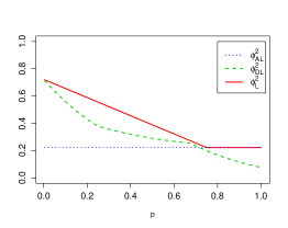
(a) Relationship between $\phi^{2}_{\rm AL}$, $\phi^{2}_{\rm DL}$ and $\phi^{2}_{\rm L}$.

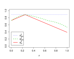
(b) Relationship between $\phi^{2}_{\rm AH}$, $\phi^{2}_{\rm DH}$ and $\phi^{2}_{\rm H}$.

Figure 1: Comparison of three bounds under different values of $p$.

Figure 1 shows that $\phi^{2}_{\rm L}\geq\max\{\phi^{2}_{\rm AL},\phi^{2}_{\rm DL}\}$ and $\phi^{2}_{\rm H}\leq\min\{\phi^{2}_{\rm AH},\phi^{2}_{\rm DH}\}$ under all settings of $p$, and in many situations the inequalities are strict. For $p\leq 143/200$, Ding et al. (2019)’s bound is tighter than Aronow et al. (2014)’s bound. However, for $p>143/200$, $\phi^{2}_{\rm DL}<\phi^{2}_{\rm AL}$, although covariate information is also used in the approach of Ding et al. (2019).

2.3 Estimation of the sharp bound and the confidence interval

To estimate $\phi_{\rm L}^{2}$ and $\phi_{\rm H}^{2}$ and study asymptotic properties of the proposed estimators for them, we adopt the following standard framework (Li and Ding, 2017) for theoretical development. Suppose that there is a sequence of finite populations $\mathbf{U}_{N}$ of size $N$. For each $N$, $n_{1}$ units are randomly assigned to treatment group and $n_{0}$ units to control group. As the population size $N\to\infty$, the sizes of the treatment and the control groups satisfy $n_{1}/N\to\rho_{1}$, $n_{0}/N\to\rho_{0}$ with $\rho_{1}$, $\rho_{0}\in(0,1)$ and $\rho_{1}+\rho_{0}\leq 1$. Here we assume that the number of covariate values $K$ is known and is allowed to grow at a certain rate with the population size $N$. To accommodate continuous covariates, we can stratify them and increase the number of strata with the sample size. We estimate $\pi_{k}$ and $F_{t\mid k}(y)$ with empirical probabilities $\hat{\pi}_{k}=1/n\sum_{T_{i}\in\{0,1\}}1\{w_{i}=\xi_{k}\}$ and $\hat{F}_{t\mid k}(y)=\sum_{T_{i}=t}1\{y_{ti}\leq y,w=\xi_{k}\}/\sum_{T_{i}=t}1\{w_{i}=\xi_{k}\}$, respectively. By plugging in these estimators, we obtain the following estimators for $\phi_{\rm L}^{2}$ and $\phi_{\rm H}^{2}$:

$$\hat{\phi}^{2}_{\rm L}=\sum_{k=1}^{K}\hat{\pi}_{k}\int_{0}^{1}(\hat{F}_{1\mid k}^{-1}(u)-\hat{F}_{0\mid k}^{-1}(u))^{2}du-\hat{\theta}^{2},$$ (4)

$$\hat{\phi}^{2}_{\rm H}=\sum_{k=1}^{K}\hat{\pi}_{k}\int_{0}^{1}(\hat{F}_{1\mid k}^{-1}(1-u)-\hat{F}_{0\mid k}^{-1}(u))^{2}du-\hat{\theta}^{2}.$$

These estimators involve sample conditional quantile functions $\hat{F}_{t\mid k}^{-1}(u)$, whose statistical properties are complicated in the finite population framework. Many theoretical results for conditional quantile functions in the super population framework can not be applied to the scenario we consider. Moreover, the number of covariate values $K$ is allowed to diverge as the population size, which further complicates the problem. Thus it is not trivial to analyze the asymptotic properties of these estimators. However, we observe that the first term of these estimators is actually weighted sums of the Wasserstein distances between some distributions. By invoking a representation theorem of Wasserstein distances, we are able to prove the consistency results for the estimators with a careful analysis of the error terms. See the Appendix for more details. We assume that the population $\mathbf{U}_{N}$ satisfies the following two conditions.

Condition 1.

There is some constant $C_{M}$ which does not depend on $N$ such that $1/N\sum_{i=1}^{N}y_{ti}^{4}\leq C_{M}$ for $t=0,1$.

Condition 2.

There is some constant $C_{\pi}$ which does not depend on $N$ such that $\pi_{k}\geq C_{\pi}/K$ for $k=1,\dots,K$.

Furthermore, we assume $K$ satisfies the following condition.

Condition 3.

$K^{2}\log K/N\to 0$ as $N\to\infty$.

Condition 1 requires the potential outcomes have uniformly bounded fourth moments. Condition 2 requires the proportion of units with each covariate value not to be too small. Condition 3 imposes some upper bound on the number of values the covariate may take. If the covariate $w$ is some subgroup indicator, then Condition 3 can be easily satisfied if the number of subgroups is not too large. Continuous components in $w$ can be stratified to meet Condition 3. If $w$ contains many components, then the number of covariate values may be too large even after stratifying the continuous components. In this case, one can partition units with similar covariate values into subgroups and use the subgroup label as the new covariate to apply the proposed method. Alternatively, in practice, one can first conduct dimension reduction or variable selection methods to obtain a low-dimensional covariate, and then apply the proposed method using the obtained covariate. The following theorem establishes the consistency of the bound estimators.

Theorem 2.

Under Conditions 1, 2 and 3, we have

$$(\hat{\phi}_{\rm L}^{2},\hat{\phi}_{\rm H}^{2})-(\phi_{\rm L}^{2},\phi_{\rm H}^{2})\stackrel{{\scriptstyle P}}{{\to}}0.$$

as $N\to\infty$.

Proof of this theorem is relegated to the Appendix. The lower bound $\phi^{2}_{\rm L}$ for $\phi^{2}(\tau)$ implies an upper bound for $\sigma^{2}$. Consistency result of $\hat{\phi}^{2}_{\rm L}$ is sufficient for constructing a conservative confidence interval. A conservative $1-\alpha$ confidence interval for $\theta$ is given by

$$I_{N}=\left[\hat{\theta}-q_{\frac{\alpha}{2}}\hat{\sigma}N^{-\frac{1}{2}},\hat{\theta}+q_{\frac{\alpha}{2}}\hat{\sigma}N^{-\frac{1}{2}}\right],$$ (5)

where

$$\hat{\sigma}^{2}=\left(\frac{N}{n_{1}}\hat{\phi}^{2}_{1}+\frac{N}{n_{0}}\hat{\phi}^{2}_{0}-\hat{\phi}^{2}_{L}\right)$$

and $q_{\alpha/2}$ is the upper $\alpha/2$ quantile of a standard normal distribution.

Next, we study the property of the confidence interval $I_{N}$ in (5). As discussed in (Lehmann and Romano, 2006), inference based on asymptotic results is not reassuring unless some uniform convergence results can be established. We next show that $I_{N}$ is uniformly asymptotically level $1-\alpha$ over a class of finite populations. For some constants $L_{1},L_{2},L_{3}>0$, we introduce the following class of finite populations

$$\mathcal{P}_{N} =\Bigg{\{}\mathbf{U}_{N}^{*}=(y_{1}^{*},y_{0}^{*},w^{*}):\ \text{$\mathbf{U}_{N}^{*}$ is of size $N$, and}$$ (6)

$$\qquad\text{(a)}\ \frac{1}{N}\sum_{i=1}^{N}y_{ti}^{*4}\leq L_{1};\quad\text{(b)}\ \phi^{2}(y_{t}^{*})\geq L_{2};\quad\text{(c)}\ P(w^{*}=\xi_{k})\geq\frac{L_{3}}{K}$$

$$\qquad\text{for $t=0,1$ and $k=1,\dots,K$}\Bigg{\}}.$$

Under Conditions 1 and 2, if the variances of the potential outcomes are bounded away from zero, then $\mathbf{U}_{N}$ belongs to $\mathcal{P}_{N}$ for some $L_{1}$, $L_{2}$ and $L_{3}$. Constraint (a) in the definition of $\mathcal{P}_{N}$ requires the fourth moments of the potential outcomes to be uniformly bounded. Bounded fourth moments are required for theoretical development in many existing works (Freedman, 2008a, b). Constraint (b) requires the variance of the potential outcomes to be bounded away from zero. According to Cauchy-Schwartz inequality and some straightforward calculations, Constraint (b) implies that the variance of $\sqrt{N}(\hat{\theta}-\theta)$ is bounded away from zero at least for sufficiently large $N$ if $\mathbf{U}_{N}\in\mathcal{P}_{N}$. Constraint (c) requires units with each covariate value not to be too rare. Constraints (b) and (c) ensure that the the denominator of some quantities appears in the theoretical analysis are not too small, which is important to establish the desired properties. The set $\mathcal{P}_{N}$ contains a large class of finite populations. For an illustration, suppose $(y_{1i},y_{0i},w_{i})$, $i=1,\dots,n$, are independent and identically distributed observations of some random variables $(Y_{1},Y_{0},W)$. Then according to the strong law of large number, $\mathbf{U}_{N}$ belongs to $\mathcal{P}_{N}$ for sufficiently large $N$ with probability one as long as $(Y_{1},Y_{0},W)$ satisfies $E[Y_{t}^{4}]<L_{1}$, ${\rm var}[Y_{t}]>L_{2}$ and $\mathbb{P}(W=\xi_{k})>L_{3}/K$ for $t=0,1$ and $k=1,\dots,K$.

Next, we show that $I_{N}$ has uniformly asymptotically guaranteed coverage rate over $\mathcal{P}_{N}$ for any $L_{1},L_{2},L_{3}>0$.

Theorem 3.

Under Condition 3, the confidence interval $I_{N}$ in (5) is uniformly asymptotically level $1-\alpha$ over $\mathcal{P}_{N}$ for any $L_{1},L_{2},L_{3}>0$, that is

$$\mathop{\lim\inf}_{N\to\infty}\inf_{\mathbf{U}_{N}\in\mathcal{P}_{N}}\mathbb{P}(\theta\in I_{N})\geq 1-\alpha.$$

Proof of this theorem is in the Appendix.

3 Sharp variance bound for the Wald estimator

3.1 Sharp bound for the unidentifiable term in the variance

In the previous section, we discuss the variance bound in completely randomized experiments with perfect compliance where each unit takes the treatment assigned by the randomization procedure. However, noncompliance often arises in randomized experiments. In the presence of noncompliance, some units may take the treatment different from the assigned treatment following their own will or for other reasons. For each unit $i$ and $t=0,1$, we let $d_{ti}\in\{0,1\}$ denote the treatment that unit $i$ actually takes if assigned to treatment $t$. In this case, the units can be classified into four groups according to the value of $(d_{1i},d_{0i})$ (Angrist et al., 1996; Frangakis and Rubin, 2002),

$$g_{i}=\left\{\begin{array}[]{lcl}\text{Alway Taker}\ (\rm a)&&\text{if}\ d_{1i}=1\ \text{and}\ d_{0i}=1,\\ \text{Complier}\ (\rm c)&&\text{if}\ d_{1i}=1\ \text{and}\ d_{0i}=0,\\ \text{Never Taker}\ (\rm n)&&\text{if}\ d_{1i}=0\ \text{and}\ d_{0i}=0,\\ \text{Defier}\ (\rm d)&&\text{if}\ d_{1i}=0\ \text{and}\ d_{0i}=1.\\ \end{array}\right.$$

Let $g=(g_{1},\dots,g_{N})$. Then the characteristics of the population can be viewed as a matrix $\mathbf{U}_{\rm c}=(y_{1},y_{0},w,g)$ where $y_{1}$, $y_{0}$ and $w$ are defined in Section 2. For $t=0,1$, $k=1,\dots,K$ and $h=\rm a,c,n,d$, let $F_{t\mid(k,h)}(y)=P(y_{t}\leq y\mid w=\xi_{k},g=h)$, $\pi_{k\mid h}=P(w=\xi_{k}\mid g=h)$ and $\pi_{h}=P(g=h)$.

In this section, we maintain the following standard assumptions for analyzing the randomized experiment with noncompliance.

Assumption 1.

(i) Monotonicity:$d_{1i}\geq d_{0i}$; (ii) exclusion restriction: $y_{1i}=y_{0i}$ if $d_{1i}=d_{0i}$; (iii) strong instrument: $\pi_{\rm c}\geq C_{0}$ where $C_{0}$ is a positive constant.

Assumption 1 (i) rules out the existence of defiers and is usually easy to assess in many situations. For example, it holds automatically if units in the control group do not have access to the treatment. Assumption 1 (ii) means that the treatment assignment affect the potential outcome only through affecting the treatment a unit actually receive. Assumption 1 (iii) assures the existence of compliers. Assumption 1 is commonly adopted to identify the causal effect in the presence of noncompliance. See Angrist et al. (1996); Abadie (2003) for more detailed discussions of Assumption 1. In the randomized experiment with noncompliance, the parameter of interest is the local average treatment effect (LATE) (Angrist et al., 1996; Abadie, 2003),

$$\theta_{\rm c}=\frac{\sum_{i=1}^{N}\tau_{i}1\{g_{i}={\rm c}\}}{\sum_{i=1}^{N}1\{g_{i}={\rm c}\}},$$

which is the average effect of treatment in the compliers.

Under the monotonicity and exclusion restriction, we have $1\{g_{i}={\rm c}\}=d_{1i}-d_{0i}$ and $(d_{1i}-d_{0i})\tau_{i}=\tau_{i}=y_{1i}-y_{0i}$. Thus

$$\pi_{\rm c}=\frac{1}{N}\sum_{i=1}^{N}1\{g_{i}={\rm c}\}=\frac{1}{N}\sum_{i=1}^{N}(d_{1i}-d_{0i})=\mu(d_{1})-\mu(d_{0}),$$

$$\frac{1}{N}\sum_{i=1}^{N}(d_{1i}-d_{0i})\tau_{i}=\frac{1}{N}\sum_{i=1}^{N}\tau_{i}=\mu(\tau),$$

and $\theta_{\rm c}=\pi_{\rm c}^{-1}\theta$. Hence $\theta_{\rm c}$ can be estimated by the “Wald estimator”,

$$\hat{\theta}_{\rm c}=\hat{\pi}_{\rm c}^{-1}\hat{\theta}$$

where $\hat{\theta}=\sum_{T_{i}=1}y_{1i}/n_{1}-\sum_{T_{i}=0}y_{0i}/n_{0}$ and $\hat{\pi}_{\rm c}=\sum_{T_{i}=1}d_{1i}/n_{1}-\sum_{T_{i}=0}d_{0i}/n_{0}$. Let $z_{i}=(y_{1i},y_{0i},d_{1i},d_{0i})^{{\mathrm{\scriptscriptstyle T}}}$, $\bar{z}=\sum_{i=1}^{N}z_{i}/N$ and

$$V_{N}=\frac{1}{N}\sum_{i=1}^{N}(z_{i}-\bar{z})(z_{i}-\bar{z})^{{\mathrm{\scriptscriptstyle T}}}.$$

The asymptotic normality is established under the following regularity condition.

Condition 4.

There is some constant $C_{\lambda}$ which does not dependent on $N$ such that the eigenvalues of $V_{N}$ is not smaller than $C_{\lambda}$.

Now we are ready to state the asymptotic normality result.

Theorem 4.

Under Assumption 1 and Conditions 1, 4, we have

$$\sqrt{N}\sigma_{\rm c}^{-1}(\hat{\theta}_{\rm c}-\theta_{\rm c})\overset{d}{\to}N(0,1)$$

provided $\sigma^{2}_{\rm c}$ is bounded away from zero, where

$$\sigma^{2}_{\rm c}=\frac{1}{\pi_{\rm c}^{2}}\left(\frac{N}{n_{1}}\phi^{2}(\tilde{y}_{1})+\frac{N}{n_{0}}\phi^{2}(\tilde{y}_{0})-\phi^{2}(\tilde{\tau})\right),$$

$\tilde{y}_{t}=(y_{t1}-\theta_{\rm c}d_{t1},\dots,y_{tN}-\theta_{\rm c}d_{tN})^{\mathrm{\scriptscriptstyle T}}$ for $t=0,1$ and $\tilde{\tau}=\tilde{y}_{1}-\tilde{y}_{0}$.

Proof of this theorem is in the Appendix. Let $\hat{y}_{ti}=y_{ti}-\hat{\theta}_{\rm c}d_{ti}$, then under the conditions of Theorem 4, $\phi^{2}(\tilde{y}_{t})$ can be consistently estimated by

$$\check{\phi}^{2}_{t}=\frac{1}{n_{t}-1}\sum_{T_{i}=t}\Big{(}\hat{y}_{ti}-\frac{1}{n_{t}}\sum_{T_{j}=t}\hat{y}_{tj}\Big{)}^{2},$$ (7)

and $\pi_{\rm c}$ can be consistently estimated by $\hat{\pi}_{\rm c}$. However, analogous to $\phi^{2}(\tau)$, $\phi^{2}(\tilde{\tau})$ is unidentifiable. Here we construct a sharp bound for $\phi^{2}(\tilde{\tau})$ using covariate information. It should be pointed out that the sharp bound has not been obtained even in the absence of covariates. Define $\tilde{F}_{t\mid k}(y)=P(\tilde{y}_{t}\leq y\mid w=\xi_{k},g={\rm c})$ be a set of lower bounds for $\phi^{2}(\tilde{\tau})$. Let $\tilde{\mathcal{B}}_{\rm L}=\{\tilde{b}_{\rm L}:\text{$\tilde{b}_{\rm L}$ is a functional of $\pi_{\rm c}$, $\pi_{k\mid\rm c}$ and $\tilde{F}_{t\mid k}$ for $t=0,1$ and $k=1,\dots,K$};\tilde{b}_{\rm L}\leq\phi^{2}(\tilde{\tau})\}$. Define the set of upper bounds $\tilde{\mathcal{B}}_{\rm H}$ similarly. Then we can establish the following sharp bound for $\phi^{2}(\tilde{\tau})$.

Theorem 5.

A bound for $\phi^{2}(\tilde{\tau})$ is $[\tilde{\phi}^{2}_{\rm L},\tilde{\phi}^{2}_{\rm H}]$ where

$$\tilde{\phi}^{2}_{\rm L}=\sum_{k=1}^{K}\pi_{\rm c}\pi_{k\mid\rm c}\int_{0}^{1}(\tilde{F}_{1\mid k}^{-1}(u)-\tilde{F}_{0\mid k}^{-1}(u))^{2}du,$$

$$\tilde{\phi}^{2}_{\rm H}=\sum_{k=1}^{K}\pi_{\rm c}\pi_{k\mid\rm c}\int_{0}^{1}(\tilde{F}_{1\mid k}^{-1}(u)-\tilde{F}_{0\mid k}^{-1}(1-u))^{2}du.$$

Moreover, the bound is sharp in the sense that $\tilde{\phi}_{\rm L}^{2}$ is the largest lower bound in $\tilde{\mathcal{B}}_{\rm L}$ and $\tilde{\phi}_{\rm H}^{2}$ is the smallest upper bounds in $\tilde{\mathcal{B}}_{\rm H}$.

See the Appendix for the proof of this theorem. If there is no covariate, we let $K=1$, $\xi_{1}=1$ and define $w_{i}=1$ for $i=1,\dots,N$, then we can obtain a bound without covariates, which has not been considered in the literature.

3.2 Estimation of the sharp bound and the confidence interval

To estimate the bounds, we need to estimate $\pi_{\rm c}$, $\pi_{k\mid\rm c}$, and $\tilde{F}_{t\mid k}(y)$. Here $\pi_{\rm c}$ can be estimated by $\hat{\pi}_{\rm c}$. We let

$$\hat{\lambda}_{1k}=\frac{1}{n_{1}}\sum_{T_{i}=1}d_{1i}1\{w_{i}=\xi_{k}\}-\frac{1}{n_{0}}\sum_{T_{i}=0}d_{0i}1\{w_{i}=\xi_{k}\}$$

$$\hat{\lambda}_{0k}=\frac{1}{n_{0}}\sum_{T_{i}=0}(1-d_{0i})1\{w_{i}=\xi_{k}\}-\frac{1}{n_{1}}\sum_{T_{i}=1}(1-d_{1i})1\{w_{i}=\xi_{k}\}.$$

Under Assumption 1, we estimate $\pi_{k\mid\rm c}$ and $\tilde{F}_{t\mid k}(y)$ with

$$\hat{\pi}_{k\mid{\rm c}}=\hat{\pi}_{\rm c}^{-1}\hat{\lambda}_{1\mid k},$$

$$\check{F}_{1\mid k}(y) =\hat{\lambda}_{1\mid k}^{-1}\Bigg{(}\frac{1}{n_{1}}\sum_{T_{i}=1}d_{1i}1\{\hat{y}_{1i}\leq y\}1\{w_{i}=\xi_{k}\}$$

$$\quad-\frac{1}{n_{0}}\sum_{T_{i}=0}d_{0i}1\{\hat{y}_{0i}\leq y\}1\{w_{i}=\xi_{k}\}\Bigg{)}$$

and

$$\check{F}_{0\mid k}(y) =\hat{\lambda}_{0\mid k}^{-1}\Bigg{(}\frac{1}{n_{0}}\sum_{T_{i}=0}(1-d_{0i})1\{\hat{y}_{0i}\leq y\}1\{w_{i}=\xi_{k}\}$$

$$\quad-\frac{1}{n_{1}}\sum_{T_{i}=1}(1-d_{1i})1\{\hat{y}_{1i}\leq y\}1\{w_{i}=\xi_{k}\}\Bigg{)}$$

where $\hat{y}_{ti}=y_{ti}-\hat{\theta}_{\rm c}d_{ti}$ for $t=0,1$, and $i=1,\dots,N$.

We then obtain estimators for $\tilde{\phi}_{\rm L}^{2}$ and $\phi_{\rm H}^{2}$ by plugging these estimators into the expressions of Theorem 5,

$$\check{\phi}^{2}_{\rm L}=\sum_{k=1}^{K}\hat{\pi}_{\rm c}\hat{\pi}_{k\mid\rm c}\int_{0}^{1}(\check{F}_{1\mid k}^{-1}(u)-\check{F}_{0\mid k}^{-1}(u))^{2}du,$$ (8)

$$\check{\phi}^{2}_{\rm H}=\sum_{k=1}^{K}\hat{\pi}_{\rm c}\hat{\pi}_{k\mid\rm c}\int_{0}^{1}(\check{F}_{1\mid k}^{-1}(u)-\check{F}_{0\mid k}^{-1}(1-u))^{2}du.$$

The estimator $\check{F}_{t\mid k}(y)$ may not be monotonic with respect to $y$, which brings about some difficulties for theoretical analysis. However, $\check{F}_{t\mid k}^{-1}(u)$ is still well defined, and in the next theorem we show that the non-monotonicity of $\check{F}_{t\mid k}(y)$ does not diminish the consistency of $\check{\phi}_{\rm L}^{2}$ and $\check{\phi}_{\rm H}^{2}$.

In the following asymptotic analysis, we denote $\mathbf{U}_{\rm c}$ by $\mathbf{U}_{{\rm c},N}$. We assume that $\mathbf{U}_{{\rm c},N}$ satisfies Assumption 1, Condition 1 and the following two conditions. The following conditions are modified versions of Conditions 2 and 3 in the presence of noncompliance.

Condition 5.

There is some constant $C_{\pi,{\rm c}}$ which does not depend on $N$ such that $\pi_{k\mid{\rm c}}\pi_{\rm c}\geq C_{\pi,{\rm c}}/K$ for $k=1,\dots,K$.

Condition 6.

$K^{2}\log K\max\{C_{N}^{4},1\}/N\to 0$ as $N\to\infty$, where $C_{N}=\max_{t,i}|y_{ti}|$.

Then we are ready to establish the consistency of the estimators proposed in (8).

Theorem 6.

Under Assumption 1 and Conditions 1, 5, 6, we have

$$(\check{\phi}_{\rm L}^{2},\check{\phi}_{\rm H}^{2})-(\tilde{\phi}_{\rm L}^{2},\tilde{\phi}_{\rm H}^{2})\stackrel{{\scriptstyle P}}{{\to}}0.$$

Proof of this theorem is relegated to the Appendix. The lower bound $\tilde{\phi}^{2}_{\rm L}$ for $\phi^{2}(\tilde{\tau})$ implies an upper bound for $\sigma^{2}_{\rm c}$. By Theorems 4 and 6 we can construct a conservative $1-\alpha$ confidence interval for $\theta_{\rm c}$,

$$I_{{\rm c},N}=\left[\hat{\theta}_{\rm c}-q_{\frac{\alpha}{2}}\hat{\sigma}_{\rm c}N^{-\frac{1}{2}},\hat{\theta}_{\rm c}+q_{\frac{\alpha}{2}}\hat{\sigma}_{\rm c}N^{-\frac{1}{2}}\right],$$ (9)

where

$$\hat{\sigma}_{\rm c}^{2}=\frac{1}{\hat{\pi}_{\rm c}^{2}}\left(\frac{N}{n_{1}}\check{\phi}^{2}_{1}+\frac{N}{n_{0}}\check{\phi}^{2}_{0}-\check{\phi}^{2}_{L}\right)$$

and $q_{\alpha/2}$ is the upper $\alpha/2$ quantile of a standard normal distribution. We then show that $I_{{\rm c},N}$ is uniformly asymptotically level $1-\alpha$ over a class of finite populations. In the following asymptotic analysis, we denote $\mathbf{U}_{\rm c}$ by $\mathbf{U}_{{\rm c},N}$. For any finite population $\mathbf{U}_{{\rm c},N}^{*}=(y_{1}^{*},y_{0}^{*},w^{*},g^{*})$, we define $\tilde{y}_{t}^{*}$ similarly as $\tilde{y}_{t}$ for $t=0,1$. Let $\Lambda_{N}^{*}$ be the smallest eigenvalue of

$$\frac{1}{N}\sum_{i=1}^{N}(z_{i}^{*}-\bar{z}^{*})(z_{i}^{*}-\bar{z}^{*})^{{\mathrm{\scriptscriptstyle T}}},$$

where $z_{i}^{*}=(y_{1i}^{*},y_{0i}^{*},d_{1i}^{*},d_{0i}^{*})^{{\mathrm{\scriptscriptstyle T}}}$ and $\bar{z}^{*}=\sum_{i=1}^{N}z_{i}^{*}/N$. For some constants $L_{0},L_{1},L_{2},L_{3}>0$, we introduce the following class of finite populations

$$\mathcal{P}_{{\rm c},N} =\Bigg{\{}\mathbf{U}_{{\rm c},N}^{*}=(y_{1}^{*},y_{0}^{*},w^{*},g^{*}):\ \text{$\mathbf{U}_{{\rm c},N}^{*}$ is of size $N$ and satisfies}$$

$$\qquad\text{(a)}\ \text{Assumption \ref{ass:iv};}\ \text{(b)}\ \Lambda_{N}^{*}\geq L_{0};\ \text{(c)}\ \frac{1}{N}\sum_{i=1}^{N}y_{ti}^{*4}\leq L_{1};$$

$$\qquad\text{(d)}\ \phi^{2}(\tilde{y}_{t}^{*})\geq L_{2};\quad\text{(e)}\ P(w^{*}=\xi_{k}\mid g^{*}={\rm c})P(g^{*}={\rm c})\geq\frac{L_{3}}{K}$$

$$\qquad\text{for $t=0,1$ and $k=1,\dots,K$}\Bigg{\}}.$$

Constraint (a) is required for the identification of LATE. Constraint (b) is a regularity condition to ensure the asymptotic normality of $\hat{\theta}_{\rm c}$. Constraints (c), (d) and (e) are similar to those constraints in the definition of $\mathcal{P}_{N}$ in Section 2.3. $\mathcal{P}_{{\rm c},N}$ can be a large class of finite populations if $L_{0}$, $L_{2}$, $L_{3}$ are small and $L_{1}$ is large. The class of finite populations $\mathcal{P}_{{\rm c},N}$ can be related to some class of generic distributions in the same way as discussed before Theorem 3. The details are omitted here. Similar arguments as in the proof of Theorem 3 can show the following result.

Theorem 7.

Under Condition 6, the confidence interval $I_{{\rm c},N}$ in (9) is uniformly asymptotically level $1-\alpha$ over $\mathcal{P}_{{\rm c},N}$, that is

$$\mathop{\lim\inf}_{N\to\infty}\inf_{\mathbf{U}_{{\rm c},N}\in\mathcal{P}_{{\rm c},N}}\mathbb{P}(\theta\in I_{{\rm c},N})\geq 1-\alpha.$$

4 Simulations

4.1 Completely randomized experiments with perfect compliance

In this subsection, we evaluate the performance of the bounds and the estimators $\hat{\phi}_{\rm L}$, $\hat{\phi}_{\rm H}$ proposed in Section 2 via some simulations. We first generate a finite population of size $N$ by drawing i.i.d. samples from the following data generation process:

1. $W$ takes value in $\{1,2,3,4\}$ with equal probability;

2. for $w=1,2,3,4$, $Y_{1}\mid W=w\sim N(\mu_{w},\phi^{2}_{w})$, $V\mid W=w\sim N(0,6-\phi^{2}_{w})$, $Y_{1}\Perp V\mid W$ and $Y_{0}=0.3Y_{1}+V$ where $(\mu_{1},\mu_{2},\mu_{3},\mu_{4})=(3,0,-2,4)$ and $(\phi^{2}_{1},\phi^{2}_{2},\phi^{2}_{3},\phi^{2}_{4})=(2,1.5,5,4)$.

The generated values are viewed as the fixed finite population. We take $N=400,800$ and $2000$, respectively, to demonstrate the performance of the proposed method under different population sizes. The following table exhibits the $\phi^{2}(\tau)$ and the true value of different bounds under different population sizes.

Table 1: Bounds $\phi^{2}_{\rm AL}$, $\phi^{2}_{\rm AH}$, $\phi^{2}_{\rm DL}$, $\phi^{2}_{\rm DH}$, $\phi^{2}_{\rm L}$, $\phi^{2}_{\rm H}$ and the true value of $\phi^{2}(\tau)$ under different population sizes

	$\phi^{2}_{\rm AL}$	$\phi^{2}_{\rm AH}$	$\phi^{2}_{\rm DL}$	$\phi^{2}_{\rm DH}$	$\phi^{2}_{\rm L}$	$\phi^{2}_{\rm H}$	$\phi^{2}(\tau)$
$N=400$	0.98	58.14	1.02	58.04	9.04	42.92	16.72
$N=800$	0.78	54.79	0.74	54.76	8.83	40.53	17.70
$N=2000$	0.88	58.23	0.86	58.22	9.14	42.25	18.56

It can be seen that the intervals $[\phi_{\rm AL}^{2},\phi_{\rm AH}^{2}]$, $[\phi_{\rm DL}^{2},\phi_{\rm DH}^{2}]$, $[\phi_{\rm L}^{2},\phi_{\rm H}^{2}]$ all contain $\phi^{2}(\tau)$ and hence all the bounds are valid. Under all population sizes, the lower bound $\phi_{\rm L}^{2}$ is much larger than the other two lower bounds, and the upper bound $\phi_{\rm L}^{2}$ is much smaller than the other two upper bounds.

The above results show the effectiveness of our bounds on the population level. Next, we consider the performance of the proposed bound estimators in completely randomized experiments. In the simulation, half of the units are randomly assigned to the treatment group while the other half are assigned to the control group. Then we estimate the proposed bounds with the estimators defined in (4). The randomized assignment is repeated for $1000$ times. The root mean square error (RMSE) of the bound estimators under different $N$ is summarized in Table 2. The RMSE of the bound estimators decreases as the sample size increases, which confirms the consistency result in Theorem 2.

Table 2: RMSE of the estimators for $\phi^{2}_{\rm L}$ and $\phi^{2}_{\rm H}$ under different population sizes ($n_{1}=n_{0}=N/2$)

	$N=400$	$N=800$	$N=2000$
$\phi^{2}_{\rm L}$	1.71	0.87	0.66
$\phi^{2}_{\rm H}$	2.31	1.36	1.00

Next, we evaluate the performance of the bound estimators in constructing confidence intervals (CIs). Different CIs can be constructed based on the asymptotic normality in (1) and different lower bounds for $\phi^{2}(\tau)$. To obtain the CIs, we use $\hat{\phi}_{t}^{2}$ defined in (2) to estimate $\phi^{2}(y_{t})$ for $t=0,1$, and replace $\phi^{2}(\tau)$ in $\sigma^{2}$ by the estimators of different lower bounds. Bounds of Aronow et al. (2014) and Ding et al. (2019) are estimated by plug-in estimators as suggested in these works, and the proposed lower bound is estimated by the estimators defined in (4). The average width (AW) and coverage rate (CR) of $95\%$ CIs based on the naive lower bound zero (Neyman, 1990), the estimator of $\phi^{2}_{\rm AL}$ (Aronow et al., 2014), the estimator of $\phi^{2}_{\rm DL}$ (Ding et al., 2019) and the estimator of $\phi^{2}_{\rm L}$ are listed as follows:

Table 3: Average widths (AWs) and coverage rates (CRs) of 95% CIs based on the naive bound, $\phi^{2}_{\rm AL}$, $\phi^{2}_{\rm DL}$ and $\phi^{2}_{\rm L}$ under different population sizes ($n_{1}=n_{0}=N/2$)

Method	naive		$\phi^{2}_{\rm AL}$		$\phi^{2}_{\rm DL}$		$\phi^{2}_{\rm L}$
	AW	CR	AW	CR	AW	CR	AW	CR
$N=400$	1.511	98.0%	1.495	97.8%	1.493	97.8%	1.383	96.6%
$N=800$	1.033	97.8%	1.025	97.7%	1.025	97.7%	0.945	96.7%
$N=2000$	0.674	98.4%	0.668	98.3%	0.668	98.3%	0.619	97.3%

The CIs based on the estimator of $\phi_{\rm L}^{2}$ are the shortest, and the corresponding coverage rate is the closest to $95\%$ among the four CIs under all population sizes. See the Appendix for more simulation results on the performance of the proposed CI.

4.2 Completely randomized experiments with noncompliance

Here we show the simulation performance of the bounds and the estimators $\check{\phi}_{\rm L}$, $\check{\phi}_{\rm H}$ proposed in Section 3. First, we generate finite populations of size $N=400,800$ and $2000$ by drawing i.i.d. samples from the following data generation process:

1. generate the compliance type $G\in\{{\rm a,c,n}\}$ with the probability that $G={\rm a}$, $\rm c$ and $\rm n$ being $0.2$, $0.7$ and $0.1$, respectively;

2. for $h=\rm a,c$ and $\rm n$, the conditional distribution $W\mid G=h$ has probability mass $p_{1h}$, $p_{2h}$, $p_{3h}$ and $p_{4h}$ at $1,2,3,4$, respectively, where $(p_{1\rm a},p_{2\rm a},p_{3\rm a},p_{4\rm a})=(0.15,0.2,0.3,0.35)$, $(p_{1\rm c},p_{2\rm c},p_{3\rm c},p_{4\rm c})=$
   $(0.25,0.25,0.25,0.25)$ and $(p_{1\rm n},p_{2\rm n},p_{3\rm n},p_{4\rm n})=(0.35,0.3,0.2,0.15)$;

3. for $w=1,2,3,4$, $Y_{1}\mid W=w\sim N(\mu_{w},\phi^{2}_{w})$ where $(\mu_{1},\mu_{2},\mu_{3},\mu_{4})=(3,0,-2,4)$ and $(\phi^{2}_{1},\phi^{2}_{2},\phi^{2}_{3},\phi^{2}_{4})=(2,1.5,5,4)$;

4. $Y_{0}\mid G={\rm c},W=w\sim N(0.3w,6-\phi^{2}_{w})$ and $Y_{0}=Y_{1}$ if $G=\rm a$ or $\rm n$.

As stated behind Theorem 5, the theorem can also provide a bound without using the covariate. So to illustrate the usefulness of the covariate, here we compare the bounds constructed using and without using the covariate. In the following, the lower bound using and without using the covariate is denoted by “LC” and “LNC”, and the upper bound using and without using the covariate is denoted by “HC” and “HNC”. As in Section 4.1, half of the units are randomly assigned to the treatment group while the other half are assigned to the control group. Then we estimate the bounds for each of these random assignments with the estimators proposed in (8). The randomized assignment is repeated for $1000$ times. In the simulation $\phi^{2}(\tilde{\tau})$ equals to $9.97,10.41$ and $9.56$ when $N=400,600$ and $2000$, respectively. The following table exhibits the true values of different bounds and the RMSE of their estimators under different population sizes.

Table 4: Bounds using and without using the covariate and the RMSE of their estimators under different population sizes. LNC: lower bound without covariate; HNC: upper bound without covariate; LC: lower bound with covariate; HC: upper bound with covariate ($n_{1}=n_{0}=N/2$)

	LNC		HNC		LC		HC
	Value	RMSE	Value	RMSE	Value	RMSE	Value	RMSE
$N=400$	0.78	0.75	40.05	5.41	9.82	4.62	29.42	5.94
$N=800$	0.73	0.45	39.61	3.49	10.42	3.92	28.79	5.35
$N=2000$	0.72	0.27	37.19	2.10	9.52	2.45	28.45	4.55

Table 4 shows that LC is much larger than LNC and HC is much smaller than HNC, which shows that the covariate is quite useful in sharpening the bounds. The RMSE of different bounds generally decreases as the sample size increases and this validates the consistency result in Theorem 6.

Next, we construct CIs based on the asymptotic normality in Theorem 4 and different lower bounds for $\phi^{2}(\tilde{\tau})$. To obtain the CIs, we use $\check{\phi}_{t}^{2}$ defined in (7) to estimate $\phi^{2}(\tilde{y}_{t})$ for $t=0,1$ and replace $\phi^{2}(\tilde{\tau})$ in $\sigma_{\rm c}^{2}$ by the estimators of different lower bounds. The following table summarizes the average width (AW) and coverage rate (CR) of $95\%$ CIs based on the naive lower bound zero, and the estimator of lower bounds in Theorem 5 using and without using the covariate.

Table 5: Average widths (AWs) and coverage rates (CRs) of 95% CIs based on the naive bound, HNL and HL under different population sizes. LNC: lower bound without covariate; LC: lower bound with covariate ($n_{1}=n_{0}=N/2$)

Method	naive		LNC		LC
	AW	CR	AW	CR	AW	CR
$N=400$	2.188	98.5%	2.168	98.4%	1.990	97.3%
$N=800$	1.553	97.9%	1.542	97.8%	1.399	96.4%
$N=2000$	0.980	98.2%	0.973	98.2%	0.893	96.6%

The results show that the CIs based on the estimator of LC is the shortest, and the corresponding coverage rate is closest to $95\%$ among the three CIs under all population sizes. This demonstrates the usefulness of covariate in constructing CIs.

5 Real data applications

5.1 Application to ACTG protocol 175

In this section, we apply our approach proposed in Section 2 to a dataset from the randomized trial ACTG protocol 175 (Hammer et al., 1996) for illustration. Data used in this subsection are available from the R package “speff2trial” (https://cran.r-project.org/web/ packages/speff2trial/index.
html). The ACTG 175 study evaluated four therapies in human immunodeficiency virus infected subjects whose CD4 cell counts (a measure of immunologic status) are from 200 to 500 $\rm mm^{-3}$. Here we regard the 2139 enrolled subjects as a finite population and consider two treatment arms: the standard zidovudine monotherapy (denoted by “arm 0”) and the combination therapy with zidovudine and didanosine (denoted by “arm 1”). The parameter of interest is the average treatment effect of the combination therapy on the CD8 cell count measured at $20\pm 5$ weeks post baseline compared to the monotherapy. In the randomized trial, 532 subjects are randomly assigned to arm 0 and 522 subjects are randomly assigned to arm 1. The available covariate is the age of each subject. In order to meet Condition 3, we divide people into $\lfloor N^{1/4}\rfloor=6$ groups according to age, with the first group less than 20 years old, the second group between 21 and 30 years old, the third group between 31 and 40 years old, the fourth group between 41 and 50 years old, the fifth group between 51 and 60 years old and the last group older than 60 years old. We then use the age group, gender and antiretroviral history as covariates and apply our method proposed in Section 2. The proposed bounds $\phi^{2}_{\rm L}$ and $\phi^{2}_{\rm H}$ are estimated by the estimators defined in (4). We also estimate the bounds proposed in the literature(Aronow and Middleton, 2013; Ding et al., 2019). Bounds $\phi^{2}_{\rm AL}$, $\phi^{2}_{\rm AH}$, $\phi^{2}_{\rm DL}$, $\phi^{2}_{\rm DH}$ are estimated by plug-in estimators as suggested in Aronow et al. (2014) and Ding et al. (2019). The estimates of the lower bounds $\phi^{2}_{\rm AL}$, $\phi^{2}_{\rm DL}$ and $\phi^{2}_{\rm L}$ are $0.12$, $0.27$ and $4.75$, respectively; the estimates of the upper bounds $\phi^{2}_{\rm AH}$, $\phi^{2}_{\rm DH}$ and $\phi^{2}_{\rm H}$ are $70.79$, $69.87$ and $65.67$, respectively (values are divided by $10000$). The estimate of the proposed lower bound is the largest among the three lower bounds and the estimate of the proposed upper bound is the smallest among the three upper bounds. The $95\%$ CI constructed using zero as a lower bound for $\phi^{2}(\tau)$ is $[-13.27,92.79]$. Using the estimate of Aronow et al. (2014)’s lower bound lead to the CI $[-13.25,92.77]$, and Ding et al. (2019)’s lower bound lead to the CI $[-13.23,92.75]$. The CI $[-12.46,91.98]$ is obtained by using $\hat{\phi}^{2}_{\rm L}$ given in (4). The widths of the four CIs are $106.07$, $106.02$, $105.98$ and $104.44$, respectively. Comparing the CI width of the naive method using zero as the lower bound for $\phi^{2}(\tau)$ with the CI widths using the estimates of Aronow and Middleton (2013)’s, Ding et al. (2019)’s and the proposed lower bound for $\phi^{2}(\tau)$, the CI width reductions are $0.04$, $0.09$ and $1.62$, respectively. It can be seen that the reductions for the three methods are not very large comparing with the naive method. The reason may be that $N\hat{\phi}_{1}^{2}/n_{1}+N\hat{\phi}_{0}^{2}/n_{0}$ is too large compared to the estimator of the lower bound for $\phi^{2}(\tau)$ in this specific problem, where $\hat{\phi}_{1}^{2}$ and $\hat{\phi}_{0}^{2}$ are the estimators for $\phi^{2}(y_{1})$ and $\phi^{2}(y_{0})$, respectively. Notice that the CI width is proportional to $\sqrt{N\hat{\phi}_{1}^{2}/n_{1}+N\hat{\phi}_{0}^{2}/n_{0}-\hat{\phi}_{\rm B}^{2}}$, where $\hat{\phi}_{\rm B}^{2}$ is the estimator of the lower bound for $\phi^{2}(\tau)$. This implies that the lower bound estimator $\hat{\phi}_{\rm B}^{2}$ does not play a important role in the CI width if $N\hat{\phi}_{1}^{2}/n_{1}+N\hat{\phi}_{0}^{2}/n_{0}$ is much larger than $\hat{\phi}^{2}_{\rm B}$.

5.2 Application to JOBS II

In this section, we apply our approach proposed in Section 3 to a dataset from the randomized trial JOBS II (Vinokuir et al., 1995) for illustration. Data used in this subsection are available from https://www.icpsr.umich.edu/ web/ICPSR/studies/2739. The JOBS II intervention trial studied the efficacy of a job training intervention in preventing depression caused by job loss and in prompting high-quality reemployment. The treatment consisted of five half-day training seminars that enhance the participants’ job search strategies. The control group receives a booklet with some brief tips. After some screening procedures, 1801 respondents were enrolled in this study, with 552 and 1249 respondents in the control and treatment groups, respectively. Of the respondents assigned to the treatment group, only $54\%$ participated in the treatment. Thus there is a large proportion of noncompliance in this study. The parameter of interest is the LATE of the treatment on the depression score (larger score indicating severer depression). We use the gender, the initial risk status and the economic hardship as the covariates and apply our method proposed in Section 3. The estimates for $\tilde{\phi}^{2}_{\rm L}$ and $\tilde{\phi}^{2}_{\rm H}$ are $0.23$ and $0.81$, respectively. The $95\%$ CIs constructed using the naive bound zero and $\tilde{\phi}_{\rm L}$ are $[-0.2428,0.0271]$ and $[-0.2360,0.0202]$, respectively. Our method shortens the CI by $0.014$. When testing the null hypothesis that $\theta_{\rm c}=0$ against the alternative hypothesis that $\theta_{\rm c}<0$, the naive method gives the $\rm p$-value of $0.059$ while our method gives the $\rm p$-value of $0.049$. Thus our method is able to detect the treatment effect at $0.05$ significance level while the naive method is not.

6 Discussion

In this paper, we establish sharp variance bounds for the widely-used difference-in-means estimator and Wald estimator in the presence of covariates in completely randomized experiments. These bounds can help to improve the performance of inference procedures based on normal approximation. We do not impose any assumption on the support of outcomes, hence our results are general and are applicable to both binary and continuous outcomes. Variances of the difference-in-means estimator in matched pair randomized experiments (Imai, 2008) and the Horvitz-Thompson estimator in stratified randomized experiments and clustered randomized experiments (Miratrix et al., 2013; Mukerjee et al., 2018; Middleton and Aronow, 2015) share similar unidentifiable term as our consideration. Moreover, the unidentifiable phenomenon also appears in the asymptotic variance of regression adjustment estimators, see Lin (2013), Freedman (2008a), Bloniarz et al. (2016). The insights in this paper are also applicable in these settings and we do not discuss this in detail to avoid cumbersome notations. In addition, it is of great interest to extend our work to randomized experiments with other randomization schemes such as $2^{2}$ factorial design (Lu, 2017) or some other complex assignment mechanisms (Mukerjee et al., 2018).

Appendix S1 Proof of Theorem 1

Proof.

Note that

$$\phi^{2}(\tau)=\sum_{i=1}^{K}\pi_{k}\frac{1}{N_{k}}\sum_{w_{i}=\xi_{k}}(y_{1i}-y_{0i})^{2}-\mu^{2}(\tau),$$

where $N_{k}=N\pi_{k}$. Letting $a_{k}(s)=F_{1\mid k}^{-1}(s/N_{k})$ and $b_{k}(s)=F_{0\mid k}^{-1}(s/N_{k})$ for $k=1,\dots,K$ and $s=1,\dots,N_{k}$, then we have

$$\frac{1}{N_{k}}\sum_{w_{i}=\xi_{k}}(y_{1i}-y_{0i})^{2}=\frac{1}{N_{k}}\sum_{i=1}^{N_{k}}a_{k}(i)^{2}+\frac{1}{N_{k}}\sum_{i=1}^{N_{k}}b_{k}(i)^{2}-\frac{2}{N_{k}}\sum_{i=1}^{N_{k}}a_{k}(i)b_{k}(\Pi_{k}(i))$$

where $\Pi_{k}$ is a permutation on $\{1,\dots,N_{k}\}$. By the rearrangement inequality, we have

$$\sum_{i=1}^{N_{k}}a_{k}(i)b_{k}(N_{k}-k+1)\leq\sum_{i=1}^{N_{k}}a_{k}(i)b_{k}(\Pi_{k}(i))\leq\sum_{i=1}^{N_{k}}a_{k}(i)b_{k}(i).$$

Thus

$$\int_{0}^{1}(F_{1\mid k}^{-1}(u)-F_{0\mid k}^{-1}(u))^{2}du=\frac{1}{N_{k}}\sum_{i=1}^{N_{k}}(a_{k}(i)-b_{k}(i))^{2}\leq\frac{1}{N_{k}}\sum_{w_{i}=\xi_{k}}(y_{1i}-y_{0i})^{2}$$

$$\leq\frac{1}{N_{k}}\sum_{i=1}^{N_{k}}(a_{k}(i)-b_{k}(N_{k}+1-i))^{2}=\int_{0}^{1}(F_{1\mid k}^{-1}(u)-F_{0\mid k}^{-1}(1-u))^{2}du$$

This proves the bound in Theorem 1.

Next, we prove the sharpness of the bound. Let $\mathcal{U}=\{\mathbf{U}^{*}=(y_{1}^{*},y_{0}^{*},w^{*}):P(w^{*}=\xi_{k})=\pi_{k}\ \text{and}\ P(y_{t}^{*}\leq y\mid w^{*}=\xi_{k})=F_{t\mid k}(y)\ \text{for}\ t=0,1\ \text{and}\ k=1,\dots,K\}$ be the set of all populations whose covariate distribution and distributions of each potential outcome conditional on the covariate are all identical to those of $\mathbf{U}$. We first prove that the established bound can be attained by some population among $\mathcal{U}$.

For $k=1,\dots,K$, let $i_{k(1)}<\cdots<i_{k(N_{k})}$ be the indices in $\mathcal{I}_{k}=\{i:w_{i}=\xi_{k}\}$ in increasing order. Define the population $\mathbf{U}^{\rm L}$ consisting of $N$ units with two potential outcomes $y_{1i}^{\rm L}$ and $y_{0i}^{\rm L}$ and a vector of covariates $w_{i}^{\rm L}$ associated with unit $i$ for $i=1,\dots,N$. Let $y_{1i_{k(j)}}^{\rm L}=a_{k}(j)$, $y_{0i_{k(j)}}^{\rm L}=b_{k}(j)$ and $w_{i_{k(j)}}^{\rm L}=\xi_{k}$ for $k=1\dots,K$ and $j=1,\dots,N_{k}$. Let $\tau_{i}^{\rm L}=y_{1i}^{\rm L}-y_{0i}^{\rm L}$ for $i=1,\dots,N$. Then $P(y_{t}^{\rm L}\leq y\mid w^{\rm L}=\xi_{k})=F_{t\mid k}(y)$ and $P(w^{\rm L}=\xi_{k})=\pi_{k}$ for $t=0,1$, $k=1,\dots,K$ and $y\in\mathbf{R}$ and $1/N_{k}\sum_{i\in\mathcal{I}_{k}}(y_{1i}^{\rm L}-y_{0i}^{\rm L})^{2}=1/N_{k}\sum_{j=1}^{N_{k}}(a_{k}(j)-b_{k}(j))^{2}=\int_{0}^{1}(F_{1\mid k}^{-1}(u)-F_{0\mid k}^{-1}(u))^{2}du$ for $k=1,\dots,K$. Thus $\phi^{2}(\tau^{\rm L})=\phi^{2}_{\rm L}$, which attains the lower bound for $\phi^{2}(\tau)$.

Define $\mathbf{U}^{\rm H}$ similarly with $y_{1i_{k(j)}}^{\rm H}=a_{k}(j)$, $y_{1i_{k(j)}}^{\rm H}=b_{k}(N_{k}+1-j)$ and $w_{i_{k(j)}}^{\rm H}=\xi_{k}$ for $k=1\dots,K$ and $j=1,\dots,N_{k}$. Let $\tau_{i}^{\rm H}=y_{1i}^{\rm H}-y_{0i}^{\rm H}$, then $P(y_{t}^{\rm H}\leq y\mid w^{\rm H}=\xi_{k})=F_{t\mid k}(y)$ and $P(w^{\rm H}=\xi_{k})=\pi_{k}$ for $t=0,1$, $k=1,\dots,K$ and $y\in\mathbf{R}$. Moreover, $1/N_{k}\sum_{i\in\mathcal{I}_{k}}(y_{1i}^{\rm H}-y_{0i}^{\rm H})^{2}=1/N_{k}\sum_{j=1}^{N_{k}}(a_{k}(j)-b_{k}(N_{k}+1-j))^{2}=\int_{0}^{1}(F_{1\mid k}^{-1}(u)-F_{0\mid k}^{-1}(1-u))^{2}du$ for $k=1,\dots,K$. Thus $\phi^{2}(\tau^{\rm H})=\phi^{2}_{\rm H}$, which attains the upper bound for $\phi^{2}(\tau)$.

Next, we show the sharpness of the bound. We show the result for the lower bound, i.e., $\phi_{\rm L}^{2}$ is no smaller than any bound in $\mathcal{B}_{\rm L}$, and the result for the upper bound follows similarly. For any bound $b_{\rm L}$ in $\mathcal{B}_{\rm L}$, we have $b_{\rm L}=f(\pi_{1},\dots,\pi_{K},F_{0\mid 1},\dots,F_{0\mid K},F_{1\mid 1},\dots,F_{1\mid K})$ for some functional $f$ according to the definition of $\mathcal{B}_{\rm L}$. For any $\mathbf{U}^{*}$ in $\mathcal{U}$, define $\pi_{k}^{*}=P(w^{*}=\xi_{k})$ and $F_{t\mid k}^{*}(y)=P(y_{t}^{*}\leq y\mid w=\xi_{k})$ for $t=0,1$ and $k=1,\dots,K$. Let $\tau^{*}=(y_{11}^{*}-y_{01}^{*},\dots,y_{1N}^{*}-y_{0N}^{*})$. By the applying the bound to the population $\mathbf{U}^{*}$, we have

$$f(\pi_{1}^{*},\dots,\pi_{K}^{*},F_{0\mid 1}^{*},\dots,F_{0\mid K}^{*},F_{1\mid 1}^{*},\dots,F_{1\mid K}^{*})\leq\phi^{2}(\tau^{*}).$$ (S1.1)

Because $\mathbf{U}^{*}\in\mathcal{U}$, it holds that $\pi_{k}^{*}=\pi_{k}$ and $F_{t\mid k}^{*}(y)=F_{t\mid k}(y)$ for $t=0,1$. Thus (S1.1) implies that

$$b_{\rm L} =f(\pi_{1},\dots,\pi_{K},F_{0\mid 1},\dots,F_{0\mid K},F_{1\mid 1},\dots,F_{1\mid K})$$ (S1.2)

$$=f(\pi_{1}^{*},\dots,\pi_{K}^{*},F_{0\mid 1}^{*},\dots,F_{0\mid K}^{*},F_{1\mid 1}^{*},\dots,F_{1\mid K}^{*})\leq\phi^{2}(\tau^{*})$$

for any $\mathbf{U}^{*}\in\mathcal{U}$. We have shown that there is some $\mathbf{U}^{*}\in\mathcal{U}$ such that $\phi_{\rm L}^{2}=\phi^{2}(\tau^{*})$. Hence (S1.2) implies $b_{\rm L}\leq\phi_{\rm L}^{2}$ for any $b_{\rm L}\in\mathcal{B}_{\rm L}$, which completes the proof. ∎

Appendix S2 Proof of Theorem 2

Proof.

Throughout this and the following proofs, for any real number $a$ and $b$, we let $a\land b=\min\{a,b\}$, $a\lor b=\min\{a,b\}$, $a_{+}=a\land 0$ and $a_{-}=-(a\land 0)$. For any function $H$ and any constant $C$, we let

$$H_{C}(y)=\left\{\begin{array}[]{lc}0&\ y<-C\\ H(y)&\ -C\leq y<C\\ 1&\ y\geq C\end{array}\right.$$

and $H_{C}^{-1}(y)=(H_{C})^{-1}(y)$. We prove consistency of the lower bound estimator only, and the consistency for the upper bound estimator follows similarly. For any $0<\epsilon<1$, it is easy to verify that $|\hat{\theta}-\theta|\leq\min\{1/(4\theta),1/\sqrt{2}\}\epsilon$ implies $|\hat{\theta}^{2}-\theta^{2}|\leq\epsilon$. Thus $\mathbb{P}(|\hat{\theta}^{2}-\theta^{2}|>\epsilon)\leq\mathbb{P}(|\hat{\theta}-\theta|>\min\{1/(4\theta),1/\sqrt{2}\}\epsilon)\leq{\rm var}(\hat{\theta})\max\{16\theta^{2},2\}/\epsilon$ by Chebyshev’s inequality. Under Condition 1, we have $\theta\leq(2C_{\rm M})^{1/4}$ and $\sigma^{2}\leq C_{\rm M}^{1/2}(1/n_{1}+1/n_{0})N/(N-1)$ by Jensen’s inequality. Thus for any $0<\epsilon,\delta<1$, we have

$$\mathbb{P}(|\hat{\theta}^{2}-\theta^{2}|\leq\epsilon)\geq 1-\delta$$ (S2.3)

for sufficiently large $N$. Let $\hat{\pi}_{tk}=\sum_{T_{i}=t}1\{w=\xi_{k}\}/n_{t}$ for $t=0,1$ and $k=1,\dots,K$. Then for any $C>0$,

$$|\sum_{k=1}^{K}\hat{\pi}_{k}\int_{0}^{1}(\hat{F}_{1\mid k}^{-1}(u)-\hat{F}_{0\mid k}^{-1}(u))^{2}du-\sum_{k=1}^{K}\pi_{k}\int_{0}^{1}(F_{1\mid k}^{-1}(u)-F_{0\mid k}^{-1}(u))^{2}du|$$

$$\leq|\sum_{k=1}^{K}\hat{\pi}_{k}\int_{0}^{1}(\hat{F}_{1\mid k}^{-1}(u)-\hat{F}_{0\mid k}^{-1}(u))^{2}du-\sum_{k=1}^{K}\hat{\pi}_{k}\int_{0}^{1}(\hat{F}_{1\mid k,C}^{-1}(u)-\hat{F}_{0\mid k,C}^{-1}(u))^{2}du|$$

$$+|\sum_{k=1}^{K}\pi_{k}\int_{0}^{1}(F_{1\mid k}^{-1}(u)-F_{0\mid k}^{-1}(u))^{2}du-\sum_{k=1}^{K}\pi_{k}\int_{0}^{1}(F_{1\mid k,C}^{-1}(u)-F_{0\mid k,C}^{-1}(u))^{2}du|$$

$$+|\sum_{k=1}^{K}\hat{\pi}_{k}\int_{0}^{1}(\hat{F}_{1\mid k,C}^{-1}(u)-\hat{F}_{0\mid k,C}^{-1}(u))^{2}du-\sum_{k=1}^{K}\pi_{k}\int_{0}^{1}(F_{1\mid k,C}^{-1}(u)-F_{0\mid k,C}^{-1}(u))^{2}du|$$

$$\equalscolon I_{1}+I_{2}+I_{3}.$$

Hence to prove Theorem 2, it suffices to show $I_{1}+I_{2}+I_{3}\stackrel{{\scriptstyle P}}{{\to}}0$. Note that

$$I_{2} \leq|\sum_{k=1}^{K}\pi_{k}\int_{0}^{1}(F_{1\mid k}^{-1}(u)-F_{1\mid k,C}^{-1}(u))(F_{1\mid k}^{-1}(u)+F_{1\mid k,C}^{-1}(u)-F_{0\mid k}^{-1}(u)-F_{0\mid k,C}^{-1}(u))du|$$

$$+|\sum_{k=1}^{K}\pi_{k}\int_{0}^{1}(F_{0\mid k}^{-1}(u)-F_{0\mid k,C}^{-1}(u))(F_{1\mid k}^{-1}(u)+F_{1\mid k,C}^{-1}(u)-F_{0\mid k}^{-1}(u)-F_{0\mid k,C}^{-1}(u))du|$$

$$\leq\Big{(}\sum_{k=1}^{K}\pi_{k}\int_{0}^{1}(F_{1\mid k}^{-1}(u)-F_{1\mid k,C}^{-1}(u))^{2}du\Big{)}^{\frac{1}{2}}$$

$$\times\Big{(}\sum_{k=1}^{K}\pi_{k}\int_{0}^{1}(F_{1\mid k}^{-1}(u)+F_{1\mid k,C}^{-1}(u)-F_{0\mid k}^{-1}(u)-F_{0\mid k,C}^{-1}(u))^{2}du\Big{)}^{\frac{1}{2}}$$

$$+\Big{(}\sum_{k=1}^{K}\pi_{k}\int_{0}^{1}(F_{0\mid k}^{-1}(u)-F_{0\mid k,C}^{-1}(u))^{2}du\Big{)}^{\frac{1}{2}}$$

$$\times\Big{(}\sum_{k=1}^{K}\pi_{k}\int_{0}^{1}(F_{1\mid k}^{-1}(u)+F_{1\mid k,C}^{-1}(u)-F_{0\mid k}^{-1}(u)-F_{0\mid k,C}^{-1}(u))^{2}du\Big{)}^{\frac{1}{2}},$$

where the second inequality follows from Cauchy-Schwartz inequality.

Under Condition 1, we have $I_{2}\leq 8C_{M}^{3/4}/C$ because

$$\sum_{k=1}^{K}\pi_{k}\int_{0}^{1}(F_{1\mid k}^{-1}(u)-F_{1\mid k,C}^{-1}(u))^{2}du\leq\frac{1}{N}\sum_{|y_{ti}|\geq C}y_{ti}^{2}\leq\frac{C_{M}}{C^{2}}$$

for $t=0,1$ and

$$\sum_{k=1}^{K}\pi_{k}\int_{0}^{1}(F_{1\mid k}^{-1}(u)+F_{1\mid k,C}^{-1}(u)-F_{0\mid k}^{-1}(u)-F_{0\mid k,C}^{-1}(u))^{2}du$$

$$\leq 4\sum_{k=1}^{K}\pi_{k}\int_{0}^{1}[(F_{1\mid k}^{-1}(u))^{2}+(F_{1\mid k,C}^{-1}(u))^{2}+(F_{0\mid k}^{-1}(u))^{2}+(F_{0\mid k,C}^{-1}(u))^{2}]du$$

$$\leq\frac{8}{N}\sum_{i=1}^{N}y_{1i}^{2}+\frac{8}{N}\sum_{i=1}^{N}y_{0i}^{2}\leq 16\sqrt{C_{M}}.$$

By similar arguments, we have

$$I_{1} \leq\Big{(}\sum_{k=1}^{K}\hat{\pi}_{k}\int_{0}^{1}(\hat{F}_{1\mid k}^{-1}(u)-\hat{F}_{1\mid k,C}^{-1}(u))^{2}du\Big{)}^{\frac{1}{2}}$$

$$\times\Big{(}4\sum_{k=1}^{K}\hat{\pi}_{k}\int_{0}^{1}[(\hat{F}_{1\mid k}^{-1}(u))^{2}+(\hat{F}_{1\mid k,C}^{-1}(u))^{2}+(\hat{F}_{0\mid k}^{-1}(u))^{2}+(\hat{F}_{0\mid k,C}^{-1}(u))^{2}]du\Big{)}^{\frac{1}{2}}$$

$$+\Big{(}\sum_{k=1}^{K}\hat{\pi}_{k}\int_{0}^{1}(\hat{F}_{0\mid k}^{-1}(u)-\hat{F}_{0\mid k,C}^{-1}(u))^{2}du\Big{)}^{\frac{1}{2}}$$

$$\times\Big{(}4\sum_{k=1}^{K}\hat{\pi}_{k}\int_{0}^{1}[(\hat{F}_{1\mid k}^{-1}(u))^{2}+(\hat{F}_{1\mid k,C}^{-1}(u))^{2}+(\hat{F}_{0\mid k}^{-1}(u))^{2}+(\hat{F}_{0\mid k,C}^{-1}(u))^{2}]du\Big{)}^{\frac{1}{2}}.$$

Because for $t=0,1$,

$$\sum_{k=1}^{K}\hat{\pi}_{k}\int_{0}^{1}(\hat{F}_{t\mid k}^{-1}(u)-\hat{F}_{t\mid k,C}^{-1}(u))^{2}du\leq\max_{k}\frac{\hat{\pi}_{k}}{\hat{\pi}_{tk}}\frac{N}{n_{t}}\frac{1}{N}\sum_{|y_{ti}|\geq C}y_{ti}^{2}\leq\frac{N}{n_{t}}\max_{k}\frac{\hat{\pi}_{k}}{\hat{\pi}_{tk}}\frac{C_{M}}{C^{2}},$$

and

$$\sum_{k=1}^{K}\hat{\pi}_{k}\int_{0}^{1}[(\hat{F}_{1\mid k}^{-1}(u))^{2}+(\hat{F}_{1\mid k,C}^{-1}(u))^{2}+(\hat{F}_{0\mid k}^{-1}(u))^{2}+(\hat{F}_{0\mid k,C}^{-1}(u))^{2}]du$$

$$\leq\frac{N}{n_{1}\land n_{0}}\max_{t,k}\frac{\hat{\pi}_{k}}{\hat{\pi}_{tk}}\Big{(}\frac{2}{N}\sum_{i=1}^{N}y_{1i}^{2}+\frac{2}{N}\sum_{i=1}^{N}y_{0i}^{2}\Big{)}$$

$$\leq\frac{4N}{n_{1}\land n_{0}}\max_{t,k}\frac{\hat{\pi}_{k}}{\hat{\pi}_{tk}}\sqrt{C_{M}},$$

we have

$$I_{1}\leq\frac{8N}{n_{1}\land n_{0}}\max_{t,k}\frac{\hat{\pi}_{k}}{\hat{\pi}_{tk}}\frac{C_{M}^{\frac{3}{4}}}{C}.$$

For the last term $I_{3}$, we have

$$I_{3} =\left|\sum_{k=1}^{K}\hat{\pi}_{k}\int_{0}^{1}(\hat{F}_{1\mid k,C}^{-1}(u)-\hat{F}_{0\mid k,C}^{-1}(u))^{2}du-\sum_{k=1}^{K}\pi_{k}\int_{0}^{1}(F_{1\mid k,C}^{-1}(u)-F_{0\mid k,C}^{-1}(u))^{2}du\right|$$

$$\leq\left|\sum_{k=1}^{K}\hat{\pi}_{k}\Big{(}\int_{0}^{1}(\hat{F}_{1\mid k,C}^{-1}(u)-\hat{F}_{0\mid k,C}^{-1}(u))^{2}du-\int_{0}^{1}(F_{1\mid k,C}^{-1}(u)-F_{0\mid k,C}^{-1}(u))^{2}du\Big{)}\right|$$

$$+\left|\sum_{k=1}^{K}(\hat{\pi}_{k}-\pi_{k})\int_{0}^{1}(F_{1\mid k,C}^{-1}(u)-F_{0\mid k,C}^{-1}(u))^{2}du\right|$$

$$\leq\max_{k}\left|\int_{0}^{1}(\hat{F}_{1\mid k,C}^{-1}(u)-\hat{F}_{0\mid k,C}^{-1}(u))^{2}du-\int_{0}^{1}(F_{1\mid k,C}^{-1}(u)-F_{0\mid k,C}^{-1}(u))^{2}du\right|\sum_{k=1}^{K}\hat{\pi}_{k}$$

$$+\left|\sum_{k=1}^{K}(\frac{\hat{\pi}_{k}}{\pi_{k}}-1)\pi_{k}\int_{0}^{1}(F_{1\mid k,C}^{-1}(u)-F_{0\mid k,C}^{-1}(u))^{2}du\right|$$

$$\leq\max_{k}\left|\int_{0}^{1}(\hat{F}_{1\mid k,C}^{-1}(u)-\hat{F}_{0\mid k,C}^{-1}(u))^{2}du-\int_{0}^{1}(F_{1\mid k,C}^{-1}(u)-F_{0\mid k,C}^{-1}(u))^{2}du\right|$$

$$+\max_{k}\left|\frac{\hat{\pi}_{k}}{\pi_{k}}-1\right|\left|\sum_{k=1}^{K}\pi_{k}\int_{0}^{1}(F_{1\mid k,C}^{-1}(u)-F_{0\mid k,C}^{-1}(u))^{2}du\right|$$

$$\equalscolon I_{31}+I_{32}.$$

By Condition 1, we have

$$\sum_{k=1}^{K}\pi_{k}\int_{0}^{1}(F_{1\mid k,C}^{-1}(u)-F_{0\mid k,C}^{-1}(u))^{2}du$$

$$\leq 2\sum_{k-1}^{K}\pi_{k}\int_{0}^{1}(F^{-1}_{1\mid k}(u))^{2}du+2\sum_{k-1}^{K}\pi_{k}\int_{0}^{1}(F^{-1}_{0\mid k}(u))^{2}du$$

$$=2\Big{(}\frac{1}{N}\sum_{i=1}^{N}y_{1i}^{2}+\frac{1}{N}\sum_{i=1}^{N}y_{0i}^{2}\Big{)}$$

$$\leq 2\sqrt{C_{M}}.$$

Thus

$$I_{32}\leq 2\max_{k}\left|\frac{\hat{\pi}_{k}}{\pi_{k}}-1\right|\sqrt{C_{M}}.$$

For $k=1,\dots,K$, $\int_{0}^{1}(F_{1\mid k,C}^{-1}(u)-F_{0\mid k,C}^{-1}(u))^{2}du$ is the square of the Wasserstein distance induced by $L_{2}$ norm between $F_{1\mid k,C}$ and $F_{0\mid k,C}$. By the representation theorem (Bobkov and Ledoux, 2019)[Theorem 2.11],

$$\int_{0}^{1}(\hat{F}_{1\mid k,C}^{-1}(u)-\hat{F}_{0\mid k,C}^{-1}(u))^{2}du$$

$$=2\iint_{v\leq w}[(\hat{F}_{1\mid k,C}(v)-\hat{F}_{0\mid k,C}(w))_{+}+(\hat{F}_{0\mid k,C}(v)-\hat{F}_{1\mid k,C}(w))_{+}]dvdw.$$

Because $\hat{F}_{1\mid k,C}^{-1}(v)-\hat{F}_{0\mid k,C}^{-1}(w)\leq 0$ and $\hat{F}_{0\mid k,C}(v)-\hat{F}_{1\mid k,C}(w)\leq 0$ when $v<-C$ or $w\geq C$, the integral domain can be restricted to $\{-C\leq v\leq w<C\}$ without changing the integral.

Similarly, we have

$$\int_{0}^{1}(F_{1\mid k,C}^{-1}(u)-F_{0\mid k,C}^{-1}(u))^{2}du$$

$$=2\iint_{-C\leq v\leq w<C}[(F_{1\mid k,C}(v)-F_{0\mid k,C}(w))_{+}+(F_{0\mid k,C}(v)-F_{1\mid k,C}(w))_{+}]dvdw.$$

Because $|(u_{1})_{+}-(u_{2})_{+}|\leq|u_{1}-u_{2}|$ for any $u_{1}$, $u_{2}$,

$$I_{31} \leq 2\max_{k}\iint_{-C\leq v\leq w<C}[|\hat{F}_{1\mid k,C}(v)-F_{1\mid k,C}(v)|+|\hat{F}_{0\mid k,C}(v)-F_{0\mid k,C}(v)|$$

$$\phantom{\leq 2\max_{k}\iint_{-C\leq v\leq w<C}}+|\hat{F}_{1\mid k,C}(w)-F_{1\mid k,C}(w)|+|\hat{F}_{0\mid k,C}(w)-F_{0\mid k,C}(w)|]dvdw$$

$$\leq 2C^{2}\max_{k}\{\sup_{v}|\hat{F}_{1\mid k,C}(v)-F_{1\mid k,C}(v)|+\sup_{v}|\hat{F}_{0\mid k,C}(v)-F_{0\mid k,C}(v)|\}$$

$$\leq 4C^{2}\max_{t,k}\sup_{v}|\hat{F}_{t\mid k,C}(v)-F_{t\mid k,C}(v)|.$$

For any given $M$ and $t=0,1$, let $s_{tk,j}=F_{t\mid k,C}^{-1}(j/M)$. By the standard technique in the proof of Glivenko-Cantelli theorem (van der Vaart, 2000),

$$\sup_{v}|\hat{F}_{t\mid k,C}(v)-F_{t\mid k,C}(v)|\leq\max_{j}|\hat{F}_{t\mid k,C}(s_{tk,j})-F_{t\mid k,C}(s_{tk,j})|+\frac{1}{M}.$$

For $t=0,1$ and $i=1,\dots,N$, let $y_{ti}^{*}=y_{ti}1\{-C\leq y_{ti}<C\}+C1\{y_{ti}\geq C\}-C1\{y_{ti}<-C\}$. Then

$$\hat{F}_{tk,C}(s_{tk,j})-F_{tk,C}(s_{tk,j})$$

$$=\frac{1}{\hat{\pi}_{tk}}\frac{1}{n_{t}}\sum_{T_{i}=t}1\{y_{ti}^{*}\leq s_{tk,j},x=\xi_{k}\}-\frac{1}{\pi_{k}}\frac{1}{N}\sum_{i=1}^{N}1\{y_{ti}^{*}\leq s_{tk,j},x=\xi_{k}\}$$

$$=\frac{1}{\pi_{k}}\left(\frac{1}{n_{t}}\sum_{T_{i}=t}1\{y_{ti}^{*}\leq s_{tk,j},x=\xi_{k}\}-\frac{1}{N}\sum_{i=1}^{N}1\{y_{ti}^{*}\leq s_{tk,j},x=\xi_{k}\}\right)$$

$$-\frac{1}{\pi_{k}\hat{\pi}_{tk}}(\hat{\pi}_{tk}-\pi_{k})\frac{1}{n_{t}}\sum_{T_{i}=t}1\{y_{ti}^{*}\leq s_{tk,j},x=\xi_{k}\}.$$

Because

$$\left|\frac{1}{\hat{\pi}_{tk}n_{t}}\sum_{T_{i}=t}1\{y_{ti}^{*}\leq s_{tk,j},x=\xi_{k}\}\right|\leq 1,$$

we have

$$I_{31} \leq 4C^{2}\max_{t,k,j}\Big{\{}\Big{|}\frac{1}{\pi_{k}}\Big{(}\frac{1}{n_{t}}\sum_{T_{i}=t}1\{y_{ti}^{*}\leq s_{tk,j},x=\xi_{k}\}$$

$$\quad-\frac{1}{N}\sum_{i=1}^{N}1\{y_{ti}^{*}\leq s_{tk,j},x=\xi_{k}\}\Big{)}\Big{|}+\frac{1}{\pi_{k}}|\hat{\pi}_{tk}-\pi_{k}|\Big{\}}+\frac{1}{M}.$$

For any small positive number $\epsilon$, one can choose $C$ and $M$ such that $8C_{M}^{3/4}/C\leq\epsilon$ and $1/M\leq\epsilon$. Then by Hoeffding inequality for sample without replacement (Bardenet and Maillard, 2015) and the Bonferroni inequality, we have

$$\mathbb{P}\left(4C^{2}\max_{t,k,j}\Big{\{}\frac{1}{\pi_{k}}\Big{|}\frac{1}{n_{t}}\sum_{T_{i}=t}1\{y_{ti}^{*}\leq s_{tk,j},x=\xi_{k}\}-\frac{1}{N}\sum_{i=1}^{N}1\{y_{ti}^{*}\leq s_{tk,j},x=\xi_{k}\}\Big{|}\Big{\}}\geq\epsilon\right)$$

$$\leq 4MK\exp\left(-\frac{n_{1}\land n_{0}\epsilon^{2}\min_{k}\pi_{k}^{2}}{8C^{4}}\right),$$

and

$$\mathbb{P}\left(\max_{t,k}\frac{1}{\pi_{k}}|\hat{\pi}_{tk}-\pi_{k}|\geq\epsilon\right)\leq 2K\exp\left(-2n_{1}\land n_{0}\epsilon^{2}\min_{k}\pi_{k}^{2}\right).$$

By Conditions 2 and 3 the right hand side of these two inequalities converge to zero because

$$n_{1}\land n_{0}\min_{k}\pi_{k}^{2}-C^{*}\log K\geq C_{\pi}(n_{1}\land n_{0}/N)(N/K^{2})-C^{*}\log K\to\infty,$$

with $C^{*}=8C^{4}\lor(1/2)$.

Hence, for any $\delta>0$ and sufficiently large $N$, $I_{31}\leq 3\epsilon$ and

$$\max_{t,k}\left|\frac{\hat{\pi}_{k}}{\hat{\pi}_{tk}}\right|\leq\frac{1+\epsilon}{1-\epsilon}$$

with probability greater than $1-\delta$. Without loss of generality, we let $\epsilon\leq 1/3$, then $(1+\epsilon)/(1-\epsilon)\leq 2$ and for sufficiently large $N$ we have

$$\left|\sum_{k=1}^{K}\hat{\pi}_{k}\int_{0}^{1}(\hat{F}_{1\mid k}^{-1}(u)-\hat{F}_{0\mid k}^{-1}(u))^{2}du-\sum_{k=1}^{K}\int_{0}^{1}(F_{1\mid k}^{-1}(u)-F_{0\mid k}^{-1}(u))^{2}du\right|$$

$$\leq\left(\frac{4}{\rho_{1}\land\rho_{0}}+2\sqrt{C_{M}}+4\right)\epsilon$$

with probability greater than $1-\delta$. Combining this with (S2.3) completes the proof of Theorem 2. ∎

Appendix S3 Proof of Theorem 3

In this proof, we use $\epsilon,\delta$ to denote small positive numbers whose values may change from place to place. Recall the definition of $\mathcal{P}_{N}$ in (6) in the main text. We assume without loss of generality that $\mathcal{P}_{N}$ is non-empty. Under Condition 3, according to the proof of Theorem 2, for $\mathbf{U}_{N}\in\mathcal{P}_{N}$ and any $\epsilon,\delta>0$, we have $\mathbb{P}(|\hat{\phi}_{\rm L}^{2}-\phi_{\rm L}^{2}|\leq\epsilon)\geq 1-\delta$ for any $N$ larger than a threshold $T_{1}$. Note that in the proof of Theorem 2, the threshold $T_{1}$ can be chosen to be uniform in $\mathbf{U}_{N}\in\mathcal{P}_{N}$. That is, for any small positive numbers $\epsilon,\delta$, there is some $T_{1}$ such that for $N>T_{1}$ we have

$$\inf_{\mathbf{U}_{N}\in\mathcal{P}_{N}}\mathbb{P}(|\hat{\phi}_{\rm L}^{2}-\phi_{\rm L}^{2}|\leq\epsilon)\geq 1-\delta.$$ (S3.4)

Recall the definition of $\hat{\sigma}^{2}$ in Section 2.3 and the definition of $\hat{\phi}^{2}_{1}$, $\hat{\phi}^{2}_{0}$ in Section 2.1 in the main text. According to Theorem 1,

$$\mathbb{P}(\hat{\sigma}^{2}\geq\sigma^{2}-\epsilon) \geq 1-\mathbb{P}\left(\frac{N}{n_{1}}|\phi^{2}(y_{1})-\hat{\phi}^{2}_{1}|\geq\frac{\epsilon}{3}\right)-\mathbb{P}\left(\frac{N}{n_{0}}|\phi^{2}(y_{1})-\hat{\phi}^{2}_{0}|\geq\frac{\epsilon}{3}\right)$$ (S3.5)

$$\quad-\mathbb{P}\left(|\hat{\phi}_{\rm L}^{2}-\phi_{\rm L}^{2}|\geq\frac{\epsilon}{3}\right).$$

Thus for any $\epsilon,\delta>0$, there is some threshold $T_{2}$, for $N>T_{2}$, we have

$$\inf_{\mathbf{U}_{N}\in\mathcal{P}_{N}}\mathbb{P}(\hat{\sigma}^{2}\geq\sigma^{2}-\epsilon)\geq 1-\delta$$ (S3.6)

by (S3.4), (S3.5), Chebyshev’s inequality and straightforward calculation of mean and variance of $\hat{\phi}_{1}^{2}$, $\hat{\phi}_{0}^{2}$. According to the Cauchy-Schwartz inequality, we have

$$\sigma^{2} =\frac{N}{n_{1}}\phi^{2}(y_{1})+\frac{N}{n_{0}}\phi^{2}(y_{0})-\phi^{2}(\tau)$$ (S3.7)

$$\geq\frac{N}{n_{1}}\phi^{2}(y_{1})+\frac{N}{n_{0}}\phi^{2}(y_{0})-\phi^{2}(y_{1})-\phi^{2}(y_{0})$$

$$\geq L_{2}\frac{n_{0}}{n_{1}}+L_{2}\frac{n_{1}}{n_{0}}$$

$$>L_{2}$$

if $\mathbf{U}_{N}\in\mathcal{P}_{N}$. Then (S3.6) and (S3.7) imply

$$\inf_{\mathbf{U}_{N}\in\mathcal{P}_{N}}\mathbb{P}(\hat{\sigma}\geq\sigma-\epsilon)\geq 1-\delta$$ (S3.8)

for any $N>T_{3}$, where $T_{3}$ is some threshold that depends on $\epsilon$, $\delta$.

By the finite population central limit theorem (Freedman, 2008a)[Theorem 1], for any sequence of finite populations $\{\mathbf{U}_{N}\}_{N=2}^{\infty}$ such that $\mathbf{U}_{N}\in\mathcal{P}_{N}$, we have

$$\sqrt{N}\sigma^{-1}(\hat{\theta}-\theta)\stackrel{{\scriptstyle d}}{{\to}}N(0,1)$$

as $N\to\infty$. This and (S3.7) imply for any $0<\delta<\alpha<1$ and any sequence of finite populations $\{\mathbf{U}_{N}\}_{N=2}^{\infty}$ such that $\mathbf{U}_{N}\in\mathcal{P}_{N}$, there is some $0<\epsilon<\sqrt{L_{2}}$ such that

$$\mathop{\lim\inf}\limits_{N\to\infty}\mathbb{P}\left(\theta\in\left[\hat{\theta}-q_{\frac{\alpha}{2}}(\sigma-\epsilon)N^{-\frac{1}{2}},\hat{\theta}+q_{\frac{\alpha}{2}}(\sigma-\epsilon)N^{-\frac{1}{2}}\right]\right)$$ (S3.9)

$$=\mathop{\lim\inf}\limits_{N\to\infty}\mathbb{P}\left(\sqrt{N}\sigma^{-1}(\hat{\theta}-\theta)\in\left[-q_{\frac{\alpha}{2}}(1-\sigma^{-1}\epsilon),q_{\frac{\alpha}{2}}(1-\sigma^{-1}\epsilon)\right]\right)$$

$$\geq\alpha-\delta,$$

where $q_{\alpha/2}$ is the upper $\alpha/2$ quantile of a standard normal distribution. Next we show that

$$\mathop{\lim\inf}\limits_{N\to\infty}\inf_{\mathbf{U}_{N}\in\mathcal{P}_{N}}\mathbb{P}\left(\theta\in\left[\hat{\theta}-q_{\frac{\alpha}{2}}(\sigma-\epsilon)N^{-\frac{1}{2}},\hat{\theta}+q_{\frac{\alpha}{2}}(\sigma-\epsilon)N^{-\frac{1}{2}}\right]\right)\geq\alpha-\delta.$$ (S3.10)

We prove this by contradiction. If (S3.10) does not hold, then there is some $c_{*}>0$, for any $N_{0}>0$, there is some $N_{1}>N_{0}$ and $\mathbf{U}_{N_{1}}^{\prime}$ such that

$$\mathbb{P}\left(\theta\in\left[\hat{\theta}-q_{\frac{\alpha}{2}}(\sigma-\epsilon)N^{-\frac{1}{2}},\hat{\theta}+q_{\frac{\alpha}{2}}(\sigma-\epsilon)N^{-\frac{1}{2}}\right]\right)\leq\alpha-\delta-c_{*}$$

under $\mathbf{U}_{N_{1}}^{\prime}$. Following the same procedure, we can extract a subsequence $\{\mathbf{U}_{N_{m}}^{\prime}\}_{m=1}^{\infty}$ with $N_{1}<N_{2}<\dots$ and $\mathbf{U}_{N_{m}}^{\prime}\in\mathcal{P}_{N_{m}}$ such that

$$\mathbb{P}\left(\theta\in\left[\hat{\theta}-q_{\frac{\alpha}{2}}(\sigma-\epsilon)N^{-\frac{1}{2}},\hat{\theta}+q_{\frac{\alpha}{2}}(\sigma-\epsilon)N^{-\frac{1}{2}}\right]\right)\leq\alpha-\delta-c_{*}$$

under $\mathbf{U}_{N_{m}}^{\prime}$ for $m=1,2,\dots$ Then it follows that for any sequence of finite populations $\{\mathbf{U}_{N}\}_{N=2}^{\infty}$ such that $\{\mathbf{U}_{N}\}_{N=2}^{\infty}$ contains $\{\mathbf{U}_{N_{m}}^{\prime}\}_{m=1}^{\infty}$ as a subsequence, we have

$$\lim\limits_{N\to\infty}\mathbb{P}\left(\theta\in\left[\hat{\theta}-q_{\frac{\alpha}{2}}(\sigma-\epsilon)N^{-\frac{1}{2}},\hat{\theta}+q_{\frac{\alpha}{2}}(\sigma-\epsilon)N^{-\frac{1}{2}}\right]\right)\leq\alpha-\delta-c_{*},$$

which is contradict with (S3.9). This proves (S3.10). According to (S3.10), there is some threshold $T_{3}$ such that

$$\inf_{\mathcal{P}_{N}}\mathbb{P}\left(\theta\in\left[\hat{\theta}-q_{\frac{\alpha}{2}}(\sigma-\epsilon)N^{-\frac{1}{2}},\hat{\theta}+q_{\frac{\alpha}{2}}(\sigma-\epsilon)N^{-\frac{1}{2}}\right]\right)\geq\alpha-2\delta$$

for $N>T_{3}$. Combining this with (S3.6), we have

$$\inf_{\mathcal{P}_{N}}\mathbb{P}\left(\theta\in\left[\hat{\theta}-q_{\frac{\alpha}{2}}\hat{\sigma}N^{-\frac{1}{2}},\hat{\theta}+q_{\frac{\alpha}{2}}\hat{\sigma}N^{-\frac{1}{2}}\right]\right)\geq\alpha-3\delta$$

for $N>\max\{T_{2},T_{3}\}$. This proves the theorem since $\delta$ is an arbitrary small positive number.

Appendix S4 Proof of Theorem 4

Proof.

Under Conditions 1 and 4, the conditions of the finite population central limit theorem (Freedman, 2008a)[Theorem 1] is satisfied and hence

$$\sqrt{N}V_{N}^{-1}\left(\frac{1}{n_{1}}\sum_{T_{i}=1}y_{1i}-\mu(y_{1}),\frac{1}{n_{1}}\sum_{T_{i}=1}d_{1i}-\mu(d_{1}),\frac{1}{n_{0}}\sum_{T_{i}=0}y_{0i}-\mu(y_{0}),\frac{1}{n_{0}}\sum_{T_{i}=0}d_{0i}-\mu(d_{0})\right)^{{\mathrm{\scriptscriptstyle T}}}$$

converges to a multivariate normal distribution, where $V_{N}$ is defined in Condition 4. Note that we have the decomposition

$$\hat{\theta}_{\rm c}-\theta_{\rm c}=\hat{\pi}_{\rm c}^{-1}(\hat{\theta}-\hat{\pi}_{\rm c}\theta_{\rm c})=\left(\hat{\pi}_{\rm c}^{-1}-\pi_{\rm c}^{-1}\right)\left(\hat{\theta}-\hat{\pi}_{\rm c}\theta_{\rm c}\right)+\pi_{\rm c}^{-1}(\hat{\theta}-\hat{\pi}_{\rm c}\theta).$$

Under Condition 1, it is easy to show that the trace and hence the spectral norm of $V_{N}$ is bounded. By the strong instrument assumption, the fact that $V_{N}$ has bounded spectral norm and the asymptotic normality invoked before, we have

$$\hat{\pi}_{\rm c}^{-1}-\pi_{\rm c}^{-1}=O_{p}\left(\frac{1}{\sqrt{N}}\right)$$

and

$$\hat{\theta}-\hat{\pi}_{\rm c}\theta_{\rm c}=O_{p}\left(\frac{1}{\sqrt{N}}\right).$$

Hence

$$\hat{\theta}_{\rm c}-\theta_{\rm c}=\pi_{\rm c}^{-1}(\hat{\theta}-\hat{\pi}_{\rm c}\theta_{\rm c})+o_{p}\left(\frac{1}{\sqrt{N}}\right).$$

Straightforward calculation can show that $(\hat{\theta}-\hat{\pi}_{\rm c}\theta_{\rm c})/\pi_{\rm c}$ has mean zero and variance

$$\frac{1}{\pi_{\rm c}^{2}(N-1)}\left(\frac{N}{n_{1}}\phi^{2}(\tilde{y}_{1})+\frac{N}{n_{0}}\phi^{2}(\tilde{y}_{0})-\phi^{2}(\tilde{\tau})\right)=\frac{\sigma^{2}_{\rm c}}{N-1}.$$

Again by the finite population central limit theorem we have

$$\sqrt{N}\sigma_{\rm c}^{-1}(\hat{\theta}_{\rm c}-\theta_{\rm c})=\sqrt{N}\sigma_{\rm c}^{-1}\pi_{\rm c}^{-1}(\hat{\mu}(\tau)-\hat{\pi}_{\rm c}\theta_{\rm c})+o_{p}(1)\overset{d}{\to}N(0,1).$$

∎

Appendix S5 Proof of Theorem 5

Proof.

According to exclusion restriction, if $g_{i}=\rm a$ or $\rm n$, we have

$$\tilde{\tau}_{i}=y_{1i}-y_{0i}-\theta_{\rm c}(d_{1i}-d_{0i})=0.$$

By the definition of $\theta_{\rm c}$, we have $\mu(\tilde{\tau})=0$. Thus

$$\phi^{2}(\tilde{\tau})=\frac{1}{N}\sum_{i=1}^{N}\tilde{\tau}^{2}_{i}=\pi_{\rm c}\frac{1}{N_{\rm c}}\sum_{g_{i}=\rm c}\tilde{\tau}_{i}^{2}$$

where $N_{\rm c}$. Then the bound can be proved following the same arguments as in Theorem 1. Letting $\mathcal{U}_{\rm c}=\{\mathbf{U}_{\rm c}^{*}=(y_{1}^{*},y_{0}^{*},w^{*},g^{*}):\mathbf{U}_{\rm c}^{*}\text{ satisfies Assumption \ref{ass:iv}};$
$P(g^{*}=h)=\pi_{h},\ P(w^{*}=\xi_{k}\mid g^{*}=h)=\pi_{k\mid h}\ \text{and}\ P(y_{t}^{*}\leq y\mid w^{*}=\xi_{k},g^{*}=h)=F_{t\mid(k,h)}(y)\ \text{for}\ t=0,1\ \text{and}\ h={\rm a,c,n}\}$, the sharpness of the bound can be proved similarly as in Theorem 1. ∎

Appendix S6 Proof of Theorem 6

Proof.

Firstly, we provide some relationship that is useful in the proof. According to the monotonicity and exclusion restriction, we have

$$1\{g_{i}={\rm c}\}=d_{1i}-d_{0i},$$

$$(1-d_{1i})1\{\tilde{y}_{0i}\leq y\}=(1-d_{1i})1\{\tilde{y}_{1i}\leq y\}$$

and

$$d_{0i}1\{\tilde{y}_{1i}\leq y\}=d_{0i}1\{\tilde{y}_{0i}\leq y\}.$$

Thus

$$\pi_{k\mid{\rm c}}$$

$$=\frac{\sum_{i=1}^{N}1\{g_{i}={\rm c}\}1\{w_{i}=\xi_{k}\}}{\sum_{i=1}^{N}1\{g_{i}={\rm c}\}}$$

$$=\pi_{\rm c}^{-1}\left(\frac{1}{N}\sum_{i=1}^{N}d_{1i}1\{w_{i}=\xi_{k}\}-\frac{1}{N}\sum_{i=1}^{N}d_{0i}1\{w_{i}=\xi_{k}\}\right)$$

$$=\pi_{\rm c}^{-1}\left(\frac{1}{N}\sum_{i=1}^{N}(1-d_{0i})1\{w_{i}=\xi_{k}\}-\frac{1}{N}\sum_{i=1}^{N}(1-d_{1i})1\{w_{i}=\xi_{k}\}\right),$$

$$\tilde{F}_{1\mid k}(y)$$

$$=\frac{\sum_{i=1}^{N}(d_{1i}-d_{0i})1\{\tilde{y}_{1i}\leq y\}1\{w_{i}=\xi_{k}\}}{\sum_{i=1}^{N}(d_{1i}-d_{0i})1\{w_{i}=\xi_{k}\}}$$

$$=\pi_{\rm c}^{-1}\pi_{k\mid{\rm c}}^{-1}\left(\frac{1}{N}\sum_{i=1}^{N}d_{1i}1\{\tilde{y}_{1i}\leq y\}1\{w_{i}=\xi_{k}\}-\frac{1}{N}\sum_{i=1}^{N}d_{0i}1\{\tilde{y}_{1i}\leq y\}1\{w_{i}=\xi_{k}\}\right)$$

$$=\pi_{\rm c}^{-1}\pi_{k\mid{\rm c}}^{-1}\left(\frac{1}{N}\sum_{i=1}^{N}d_{1i}1\{\tilde{y}_{1i}\leq y\}1\{w_{i}=\xi_{k}\}-\frac{1}{N}\sum_{i=1}^{N}d_{0i}1\{\tilde{y}_{0i}\leq y\}1\{w_{i}=\xi_{k}\}\right),$$

and

$$\tilde{F}_{0\mid k}(y)$$

$$=\frac{\sum_{i=1}^{N}(d_{1i}-d_{0i})1\{\tilde{y}_{0i}\leq y\}1\{w_{i}=\xi_{k}\}}{\sum_{i=1}^{N}(d_{1i}-d_{0i})1\{w_{i}=\xi_{k}\}}$$

$$=\pi_{\rm c}^{-1}\pi_{k\mid{\rm c}}^{-1}\left(\frac{1}{N}\sum_{i=1}^{N}(1-d_{0i})1\{\tilde{y}_{0i}\leq y\}1\{w_{i}=\xi_{k}\}-\frac{1}{N}\sum_{i=1}^{N}(1-d_{1i})1\{\tilde{y}_{0i}\leq y\}1\{w_{i}=\xi_{k}\}\right)$$

$$=\pi_{\rm c}^{-1}\pi_{k\mid{\rm c}}^{-1}\left(\frac{1}{N}\sum_{i=1}^{N}(1-d_{0i})1\{\tilde{y}_{0i}\leq y\}1\{w_{i}=\xi_{k}\}-\frac{1}{N}\sum_{i=1}^{N}(1-d_{1i})1\{\tilde{y}_{1i}\leq y\}1\{w_{i}=\xi_{k}\}\right).$$

Since the estimators in Theorem 6 have the similar structure as those in Theorem 2, we intend to prove the consistency in a similar way. However, there are two extra difficulties. One is that $\hat{y}_{ti}\not=\tilde{y}_{ti}$ and we need to control the error introduced by using $\hat{y}_{ti}$ in place of $\tilde{y}_{ti}$ in the estimators. The other is that the estimators $\check{F}_{t\mid k}(y)$ for $t=0,1$ and $k=1,\dots,K$ are not distribution functions and thus the representation theorem (Bobkov and Ledoux, 2019)[Theorem 2.11] can not be used directly. To solve this problem, we define

$$\check{F}_{t\mid k}^{*}(y)=\sup_{v\leq y}\check{F}_{t\mid k}(v),$$

for $t=0,1$ and $k=1,\dots,K$. Then by defination, $\check{F}_{t\mid k}^{*}(y)$ is a distribution function and, for $u\in(0,1)$, $\check{F}_{t\mid k}^{*-1}(u)=\check{F}_{t\mid k}^{-1}(u)$. Hence we can use $\check{F}_{t\mid k}^{*}(y)$ instead of $\check{F}_{t\mid k}(y)$ in the representation theorem.

We prove only for the lower bound, and the consistency result for the upper bound follows similarly. Let $\lambda_{k}=\pi_{\rm c}\pi_{k\mid\rm c}$. Because $\hat{\pi}_{\rm c}\hat{\pi}_{k\mid\rm c}=\hat{\lambda}_{1k}$, to prove $\check{\phi}^{2}_{\rm L}-\tilde{\phi}^{2}_{\rm L}\stackrel{{\scriptstyle P}}{{\to}}0$, we only need to prove

$$\sum_{k=1}^{K}\hat{\lambda}_{1k}\int_{0}^{1}(\check{F}_{1\mid k}^{-1}(u)-\check{F}_{0\mid k}^{-1}(u))^{2}du-\sum_{k=1}^{K}\lambda_{k}\int_{0}^{1}(\tilde{F}_{1\mid k}^{-1}(u)-\tilde{F}_{0\mid k}^{-1}(u))^{2}du\stackrel{{\scriptstyle P}}{{\to}}0.$$

Note that

$$\left|\sum_{k=1}^{K}\hat{\lambda}_{1k}\int_{0}^{1}(\check{F}_{1\mid k}^{-1}(u)-\check{F}_{0\mid k}^{-1}(u))^{2}du-\sum_{k=1}^{K}\lambda_{k}\int_{0}^{1}(\tilde{F}_{1\mid k}^{-1}(u)-\tilde{F}_{0\mid k}^{-1}(u))^{2}du\right|$$

$$\leq\left|\sum_{k=1}^{K}\hat{\lambda}_{1k}\Big{(}\int_{0}^{1}(\check{F}_{1\mid k}^{-1}(u)-\check{F}_{0\mid k}^{-1}(u))^{2}du-\int_{0}^{1}(\tilde{F}_{1\mid k}^{-1}(u)-\tilde{F}_{0\mid k}^{-1}(u))^{2}du\Big{)}\right|$$

$$+|\sum_{k=1}^{K}(\hat{\lambda}_{1k}-\lambda_{k})\int_{0}^{1}(\tilde{F}_{1\mid k}^{-1}(u)-\tilde{F}_{0\mid k}^{-1}(u))^{2}du|$$

$$\leq\left|\sum_{k=1}^{K}\Big{(}\frac{1}{n_{1}}\sum_{T_{i}=1}d_{1i}1\{w_{i}=\xi_{k}\}\Big{)}\Big{(}\int_{0}^{1}(\check{F}_{1\mid k}^{-1}(u)-\check{F}_{0\mid k}^{-1}(u))^{2}du-\int_{0}^{1}(\tilde{F}_{1\mid k}^{-1}(u)-\tilde{F}_{0\mid k}^{-1}(u))^{2}du\Big{)}\right|$$

$$+\left|\sum_{k=1}^{K}\Big{(}\frac{1}{n_{0}}\sum_{T_{i}=0}d_{0i}1\{w_{i}=\xi_{k}\}\Big{)}\Big{(}\int_{0}^{1}(\check{F}_{1\mid k}^{-1}(u)-\check{F}_{0\mid k}^{-1}(u))^{2}du-\int_{0}^{1}(\tilde{F}_{1\mid k}^{-1}(u)-\tilde{F}_{0\mid k}^{-1}(u))^{2}du\Big{)}\right|$$

$$+\left|\sum_{k=1}^{K}\left(\frac{\hat{\lambda}_{1k}}{\lambda_{k}}-1\right)\lambda_{1k}\int_{0}^{1}(\tilde{F}_{1\mid k}^{-1}(u)-\tilde{F}_{0\mid k}^{-1}(u))^{2}du\right|$$

$$\leq 2\max_{k}\left|\int_{0}^{1}(\check{F}_{1\mid k}^{-1}(u)-\check{F}_{0\mid k}^{-1}(u))^{2}du-\int_{0}^{1}(\tilde{F}_{1\mid k}^{-1}(u)-\tilde{F}_{0\mid k}^{-1}(u))^{2}du\right|$$

$$+\max_{k}\left|\frac{\hat{\lambda}_{1k}}{\lambda_{k}}-1\right|\sum_{k=1}^{K}\lambda_{1k}\int_{0}^{1}(\tilde{F}_{1\mid k}^{-1}(u)-\tilde{F}_{0\mid k}^{-1}(u))^{2}du$$

$$\equalscolon I_{1,\rm c}+I_{2,\rm c}.$$

By Condition 1 and Assumption 1(iii), we have

$$\theta\leq\frac{1}{N}\sum_{i=1}^{N}|y_{1i}|+\frac{1}{N}\sum_{i=1}^{N}|y_{0i}|\leq 2C_{M}^{\frac{1}{4}},$$

and

$$|\theta_{\rm c}|\leq C_{0}^{-1}\left(\frac{1}{N}\sum_{i=1}^{N}|y_{1i}|+\frac{1}{N}\sum_{i=1}^{N}|y_{0i}|\right)\leq 2C_{0}^{-1}C_{M}^{\frac{1}{4}}$$

due to Jensen’s inequality. Note that $|\tilde{y}_{ti}|\leq y_{ti}+|\theta_{\rm c}|$. By Condition 1 we have

$$\sum_{k=1}^{K}\lambda_{1k}\int_{0}^{1}(\tilde{F}_{1\mid k}^{-1}(u)-\tilde{F}_{0\mid k}^{-1}(u))^{2}du \leq\frac{2}{N}\sum_{i=1}^{N}\tilde{y}_{1i}^{2}+\frac{2}{N}\sum_{i=1}^{N}\tilde{y}_{0i}^{2}$$

$$\leq\frac{4}{N}\sum_{i=1}^{N}y_{1i}^{2}+\frac{4}{N}\sum_{i=1}^{N}y_{0i}^{2}+8|\theta_{\rm c}|$$

$$\leq 8\sqrt{C_{M}}(1+2C_{0}^{-1}).$$

For any small positive $\epsilon$, according to Hoeffding inequality for sampling without replacement (Bardenet and Maillard, 2015) and the Bonferroni inequality we have

$$\mathbb{P}\left(8\sqrt{C_{M}}(1+2C_{0}^{-1})\max_{t,k}\frac{1}{\lambda_{k}}|\hat{\lambda}_{tk}-\lambda_{k}|\geq\epsilon\right)$$

$$\leq 2K\exp\left(-\frac{1}{32C_{M}(1+2C_{0}^{-1})^{2}}n_{1}\land n_{0}\epsilon^{2}\min_{k}\lambda_{k}^{2}\right)\to 0$$

by Conditions 5 and 6. Without loss of generality, we assume $\epsilon\leq 1/2$ in the proof. Thus for any $\delta>0$ and sufficiently large $N$

$$I_{2,\rm c}\leq\epsilon$$

with probability at least $1-\delta/3$.

Define $B_{N}=(C_{N}+C_{B})\lor 1$ where $C_{B}=10C_{0}^{-2}C_{M}^{1/4}$. For $\epsilon\leq B_{N}(C_{0}\land C_{M}^{1/4})$, it is easy to verify that

$$\{B_{N}|\hat{\pi}_{\rm c}-\pi_{\rm c}|<\frac{\epsilon}{2}\}\cap\{B_{N}|\hat{\theta}-\theta|<\frac{\epsilon}{2}\}\subset\{B_{N}|\hat{\theta}_{\rm c}-\theta_{\rm c}|<\epsilon\}.$$

Thus

$$\mathbb{P}\left(B_{N}|\hat{\theta}_{\rm c}-\theta_{\rm c}|\geq C_{B}\epsilon\right) \leq\mathbb{P}\left(B_{N}|\hat{\pi}_{\rm c}-\pi_{\rm c}|\geq\frac{\epsilon}{2}\right)+\mathbb{P}\left(B_{N}|\hat{\theta}-\theta|\geq\frac{\epsilon}{2}\right)$$ (S6.11)

$$\leq 4\exp\left(-\frac{2n_{1}\land n_{0}\epsilon^{2}}{B_{N}^{2}}\right)+4\exp\left(-\frac{n_{1}\land n_{0}\epsilon^{2}}{2B_{N}^{2}C_{N}^{2}}\right)$$

where the last inequality follows from the Hoeffding inequality. By Condition 6,

$$4\exp\left(-\frac{2n_{1}\land n_{0}\epsilon^{2}}{B_{N}^{2}}\right)+4\exp\left(-\frac{n_{1}\land n_{0}\epsilon^{2}}{2B_{N}^{2}C_{N}^{2}}\right)\to 0.$$

Thus for sufficiently large $N$ with probability greater than $1-\delta/3$ we have $B_{N}|\hat{\theta}_{\rm c}-\theta_{\rm c}|\leq C_{B}\epsilon$. Note that $C_{0}\leq 1$, $|\tilde{y}_{ti}|\leq y_{ti}+|\theta_{\rm c}|\leq C_{N}+2C_{0}^{-1}C_{M}^{1/4}\leq B_{N}$ and $|\hat{y}_{ti}|\leq|y_{ti}|+|\hat{\theta}_{\rm c}|\leq C_{N}+2C_{0}^{-1}C_{M}^{1/4}+C_{B}\epsilon\leq B_{N}$ when the event $\{B_{N}|\hat{\theta}_{\rm c}-\theta_{\rm c}|<C_{B}\epsilon\}$ holds. On the event $\{B_{N}|\hat{\theta}_{\rm c}-\theta_{\rm c}|<C_{B}\epsilon\}$, by the representation theorem (Bobkov and Ledoux, 2019)[Theorem 2.11], using the similar arguments as those in the proof of Theorem 2, we can show that

$$\max_{k}|\int_{0}^{1}(\check{F}_{1\mid k}^{-1}(u)-\check{F}_{0\mid k}^{-1}(u))^{2}du-\int_{0}^{1}(\tilde{F}_{1\mid k}^{-1}(u)-\tilde{F}_{0\mid k}^{-1}(u))^{2}du|$$

$$\leq 2\max_{k}\iint_{-B_{N}\leq v\leq w\leq B_{N}}[|\check{F}_{1\mid k}^{*}(v)-\tilde{F}_{1\mid k}(v)|+|\check{F}_{0\mid k}^{*}(v)-\tilde{F}_{0\mid k}(v)|$$

$$\phantom{\leq 2\max_{k}\iint_{-B_{N}\leq v\leq w\leq B_{N}}}+|\check{F}_{1\mid k}^{*}(w)-\tilde{F}_{1\mid k}(w)|+|\check{F}_{0\mid k}^{*}(w)-\tilde{F}_{0\mid k}(w)|]dvdw$$

$$\leq 4B_{N}\max_{k}\int_{-B_{N}}^{B_{N}}|\check{F}_{1\mid k}^{*}(v)-\tilde{F}_{1\mid k}(v)|dv+4B_{N}\max_{k}\int_{-B_{N}}^{B_{N}}|\check{F}_{0\mid k}^{*}(v)-\tilde{F}_{0\mid k}(v)|dv.$$ (S6.12)

Here we only analyze the first term $B_{N}\max_{k}\int_{-B_{N}}^{B_{N}}|\check{F}_{1\mid k}^{*}(v)-F_{1\mid k}(v)|dv$ and the same result can be proved similarly for the second term. Define

$$\bar{F}_{11\mid k}(y)=\frac{\hat{\lambda}_{1k}^{-1}}{n_{1}}\sum_{T_{i}=1}d_{1i}1\{\tilde{y}_{1i}\leq y\}1\{w_{i}=\xi_{k}\},$$

$$\bar{F}_{01\mid k}(y)=\frac{\hat{\lambda}_{1k}^{-1}}{n_{0}}\sum_{T_{i}=0}d_{0i}1\{\tilde{y}_{0i}\leq y\}1\{w_{i}=\xi_{k}\},$$

$$\tilde{F}_{11\mid k}(y)=\frac{\lambda_{k}^{-1}}{N}\sum_{i=1}^{N}d_{1i}1\{\tilde{y}_{1i}\leq y\}1\{w_{i}=\xi_{k}\},$$

$$\tilde{F}_{01\mid k}(y)=\frac{\lambda_{k}^{-1}}{N}\sum_{i=1}^{N}d_{0i}1\{\tilde{y}_{0i}\leq y\}1\{w_{i}=\xi_{k}\}.$$

for $k=1,\dots,K$. Let $\bar{F}_{1\mid k}(y)=\bar{F}_{11\mid k}(y)-\bar{F}_{01\mid k}(y)$, then the relationship

$$\check{F}_{1\mid k}(y)=\bar{F}_{1\mid k}(y+\hat{\theta}_{\rm c}-\theta_{\rm c})$$

holds. Because $|\sup_{v\leq y}\bar{F}_{1\mid k}(v)-\sup_{v\leq y}\tilde{F}_{1\mid k}(v)|\leq\sup_{v}|\bar{F}_{1\mid k}(v)-\tilde{F}_{1\mid k}(v)|$ and $\sup_{v\leq y}\tilde{F}_{1\mid k}(v)=\tilde{F}_{1\mid k}(y)$, we have

$$|\sup_{v\leq y}\bar{F}_{1\mid k}(v)-\bar{F}_{1\mid k}(y)|$$

$$\leq|\sup_{v\leq y}\bar{F}_{1\mid k}(v)-\sup_{v\leq y}\tilde{F}_{1\mid k}(v)|+|\bar{F}_{1\mid k}(y)-\tilde{F}_{1\mid k}(y)|$$

$$\leq 2\sup_{v}|\bar{F}_{1\mid k}(v)-\tilde{F}_{1\mid k}(v)|.$$

Hence

$$|\check{F}_{1\mid k}^{*}(y)-\tilde{F}_{1\mid k}(y)|$$

$$\leq|\sup_{v\leq y+\hat{\theta}_{\rm c}-\theta_{\rm c}}\bar{F}_{1\mid k}(v)-\bar{F}_{1\mid k}(y+\hat{\theta}_{\rm c}-\theta_{\rm c})|+|\bar{F}_{1\mid k}(y+\hat{\theta}_{\rm c}-\theta_{\rm c})-\tilde{F}_{1\mid k}(y)|$$

$$\leq 2\sup_{v}|\bar{F}_{1\mid k}(v)-\tilde{F}_{1\mid k}(v)|+|\bar{F}_{1\mid k}(y+\hat{\theta}_{\rm c}-\theta_{\rm c})-\tilde{F}_{1\mid k}(y+\hat{\theta}_{\rm c}-\theta_{\rm c})|$$

$$+|\tilde{F}_{1\mid k}(y+\hat{\theta}_{\rm c}-\theta_{\rm c})-\tilde{F}_{1\mid k}(y)|$$

$$\leq 3\sup_{v}|\bar{F}_{1\mid k}(v)-\tilde{F}_{1\mid k}(v)|+|\tilde{F}_{1\mid k}(y+\hat{\theta}_{\rm c}-\theta_{\rm c})-\tilde{F}_{1\mid k}(y)|.$$

Moreover, because

$$|\tilde{F}_{1\mid k}(y+\hat{\theta}_{\rm c}-\theta_{\rm c})-\tilde{F}_{1\mid k}(y)|$$

$$\leq|\tilde{F}_{11\mid k}(y+\hat{\theta}_{\rm c}-\theta_{\rm c})-\tilde{F}_{11\mid k}(y)|+|\tilde{F}_{01\mid k}(y+\hat{\theta}_{\rm c}-\theta_{\rm c})-\tilde{F}_{01\mid k}(y)|$$

$$\leq\lambda^{-1}_{k}\Big{(}\frac{1}{N}\sum_{i=1}^{N}d_{1i}1\{|\tilde{y}_{1i}-y|\leq|\hat{\theta}_{\rm c}-\theta_{\rm c}|\}1\{w_{i}=\xi_{k}\}$$

$$\phantom{\leq\lambda^{-1}_{k}\Big{(}}+\frac{1}{N}\sum_{i=1}^{N}d_{0i}1\{|\tilde{y}_{0i}-y|\leq|\hat{\theta}_{\rm c}-\theta_{\rm c}|\}1\{w_{i}=\xi_{k}\}\Big{)},$$

we have

$$B_{N}\max_{k}\int_{-B_{N}}^{B_{N}}|\check{F}_{1\mid k}^{*}(v)-F_{1\mid k}(v)|dv\leq 3B_{N}^{2}\max_{k}\sup_{v}|\bar{F}_{1\mid k}(v)-\tilde{F}_{1\mid k}(v)|+2B_{N}|\hat{\theta}_{\rm c}-\theta_{\rm c}|.$$

By inequality (S6.11), we have $B_{N}|\hat{\theta}_{\rm c}-\theta_{\rm c}|\leq C_{B}\epsilon$ with probability at least $1-\delta/3$ for sufficiently large $N$. Using the similar arguments as those used to analyze $I_{31}$ in the proof of Theorem 2, we can show

$$B_{N}^{2}\max_{k}\sup_{v}|\bar{F}_{1\mid k}(v)-\tilde{F}_{1\mid k}(v)|\leq\epsilon$$

with probability at least $1-\delta/6$ for sufficiently large $N$. By applying the similar arguments to the second term of expression (S6.12), we have $I_{1,\rm c}\leq(48+32C_{B})\epsilon$ with probability at least $1-2\delta/3$ for sufficiently large $N$. Thus we have proved that for any small positive numbers $\epsilon$ and $\delta$, we have $|\check{\phi}^{2}_{\rm L}-\tilde{\phi}^{2}_{\rm L}|\leq(49+32C_{B})\epsilon$ with probability at least $1-\delta$ for sufficiently large $N$ and this implies the consistency of the estimator. ∎

Appendix S7 Further simulation results

To explore the reliability of the proposed confidence intervals (CIs), we consider the case where $\phi^{2}(\tau)$ attains the lower bound $\phi_{\rm L}^{2}$. In this case, the asymptotic variance of $\sqrt{N}(\hat{\theta}-\theta)$ achieves its upper bound. According to the proof of the sharpness in Theorem 1, we can modify the finite populations considered in Section 4.1 to make $\phi^{2}(\tau)$ equal to $\phi_{\rm L}^{2}$ without changing $\pi_{k}$, $F_{1\mid k}(y)$ or $F_{0\mid k}(y)$ ($k=1,\dots,K$). Then we conducted the simulation in the same way as in Section 4.1 in the main text under the modified finite populations. The average width (AW) and coverage rate (CR) of $95\%$ CIs based on the naive lower bound zero (Neyman, 1990), the estimator of $\phi^{2}_{\rm AL}$ (Aronow et al., 2014), the estimator of $\phi^{2}_{\rm DL}$ (Ding et al., 2019) and the estimator of $\phi^{2}_{\rm L}$ are summarized in the following table.

Table S6: Average widths (AWs) and coverage rates (CRs) of 95% CIs based on the naive bound, $\phi^{2}_{\rm AL}$, $\phi^{2}_{\rm DL}$ and $\phi^{2}_{\rm L}$ under different population sizes when $\phi^{2}(\tau)$ attains the lower bound $\phi_{\rm L}^{2}$ ($n_{1}=n_{0}=N/2$)

Method	naive		$\phi^{2}_{\rm AL}$		$\phi^{2}_{\rm DL}$		$\phi^{2}_{\rm L}$
	AW	CR	AW	CR	AW	CR	AW	CR
$N=400$	1.511	96.4%	1.495	96.3%	1.493	96.3%	1.380	94.7%
$N=800$	1.033	96.6%	1.025	96.4%	1.025	96.4%	0.944	95.2%
$N=2000$	0.674	97.0%	0.669	96.9%	0.669	96.9%	0.619	95.7%

Comparing Table S6 with Table 3 in the main text, we find that the AWs are similar while the CRs are smaller in Table S6. This is because the bounds are all the same under the finite populations considered in Table S6 and Table 3, but the variance of $\hat{\theta}$ is larger here. The CI based on $\phi_{\rm L}^{2}$ is still quite reliable in this case because its CR is close to $95\%$.

We then investigate the AW and CR of the CIs in randomized experiments with noncompliance similarly. The following table summarizes the average width (AW) and coverage rate (CR) of $95\%$ CIs based on the naive lower bound zero, and the estimator of lower bounds in Theorem 5 using and without using the covariate.

Table S7: Average widths (AWs) and coverage rates (CRs) of 95% CIs based on the naive bound, HNL and HL under different population sizes when $\phi^{2}(\tilde{\tau})$ attains the lower bound $\tilde{\phi}_{\rm L}^{2}$. LNC: lower bound without covariate; HNC: upper bound without covariate; LC: lower bound with covariate; HC: upper bound with covariate ($n_{1}=n_{0}=N/2$)

Method	naive		LNC		LC
	AW	CR	AW	CR	AW	CR
$N=400$	2.186	96.7%	2.166	96.7%	1.983	94.1%
$N=800$	1.553	97.0%	1.542	96.8%	1.397	94.5%
$N=2000$	0.980	96.2%	0.973	96.0%	0.893	94.8%

It can be seen that the CI based on LC is still quite reliable even when the asymptotic variance of $\hat{\theta}_{\rm c}$ achieves its upper bound.

References

• Abadie (2003) Abadie, A. (2003). Semiparametric instrumental variable estimation of treatment response models. Journal of Econometrics 113, 231–263.
• Angrist et al. (1996) Angrist, J. D., G. W. Imbens, and D. B. Rubin (1996). Identification of causal effects using instrumental variables. Journal of the American Statistical Association 91, 444–455.
• Aronow et al. (2014) Aronow, P. M., D. P. Green, and D. K. K. Lee (2014). Sharp bounds on the variance in randomized experiments. The Annals of Statistics 42, 850–871.
• Aronow and Middleton (2013) Aronow, P. M. and J. A. Middleton (2013). A class of unbiased estimators of the average treatment effect in randomized experiments. Journal of Causal Inference 1.
• Bardenet and Maillard (2015) Bardenet, R. and O.-A. Maillard (2015). Concentration inequalities for sampling without replacement. Bernoulli 21, 1361–1385.
• Belloni et al. (2014) Belloni, A., V. Chernozhukov, and C. Hansen (2014). Inference on treatment effects after selection among high-dimensional controls. The Review of Economic Studies 81, 608–650.
• Bloniarz et al. (2016) Bloniarz, A., H. Liu, C.-H. Zhang, J. S. Sekhon, and B. Yu (2016). Lasso adjustments of treatment effect estimates in randomized experiments. Proceedings of the National Academy of Sciences 113, 7383–7390.
• Bobkov and Ledoux (2019) Bobkov, S. and M. Ledoux (2019). One-dimensional Empirical Measures, Order Statistics, and Kantorovich Transport Distances, Volume 261. American Mathematical Society.
• Chan et al. (2016) Chan, K. C. G., S. C. P. Yam, and Z. Zhang (2016). Globally efficient non-parametric inference of average treatment effects by empirical balancing calibration weighting. Journal of the Royal Statistical Society: Series B (Statistical Methodology) 78, 673–700.
• Cochran (1977) Cochran, W. G. (1977). Sampling Techniques (3 ed.). Wiley, New York.
• Ding and Dasgupta (2016) Ding, P. and T. Dasgupta (2016). A potential tale of two-by-two tables from completely randomized experiments. Journal of the American Statistical Association 111, 157–168.
• Ding et al. (2019) Ding, P., A. Feller, and L. Miratrix (2019). Decomposing treatment effect variation. Journal of the American Statistical Association 114, 304–317.
• Ding and Miratrix (2018) Ding, P. and L. W. Miratrix (2018). Model-free causal inference of binary experimental data. Scandinavian Journal of Statistics 46, 200–214.
• Frangakis and Rubin (2002) Frangakis, C. E. and D. B. Rubin (2002). Principal stratification in causal inference. Biometrics 58, 21–29.
• Freedman (2008a) Freedman, D. A. (2008a). On regression adjustments in experiments with several treatments. The Annals of Applied Statistics 2, 176–196.
• Freedman (2008b) Freedman, D. A. (2008b). On regression adjustments to experimental data. Advances in Applied Mathematics 40(2), 180–193.
• Hammer et al. (1996) Hammer, S. M., D. A. Katzenstein, M. D. Hughes, H. Gundacker, R. T. Schooley, R. H. Haubrich, W. K. Henry, M. M. Lederman, J. P. Phair, M. Niu, M. S. Hirsch, and T. C. Merigan (1996). A trial comparing nucleoside monotherapy with combination therapy in hiv-infected adults with cd4 cell counts from 200 to 500 per cubic millimeter. The New England Journal of Medicine 335, 1081 – 1090.
• Hirano et al. (2003) Hirano, K., G. W. Imbens, and G. Ridder (2003). Efficient estimation of average treatment effects using the estimated propensity score. Econometrica 71, 1161–1189.
• Hong et al. (2020) Hong, H., M. P. Leung, and J. Li (2020). Inference on finite-population treatment effects under limited overlap. The Econometrics Journal 23, 32–47.
• Imai (2008) Imai, K. (2008). Variance identification and efficiency analysis in randomized experiments under the matched-pair design. Statistics in Medicine 27, 4857–4873.
• Imbens (2004) Imbens, G. W. (2004). Nonparametric estimation of average effects under exogeneity: a review. The Review of Economics and Statistics 86, 4–29.
• Imbens and Rosenbaum (2005) Imbens, G. W. and P. R. Rosenbaum (2005). Robust accurate confidence intervals with a weak instrument. Journal of the Royal Statistical Society:Series A (Statistics in Society) 25, 305–327.
• Kallus (2018) Kallus, N. (2018). Optimal a priori balance in the design of controlled experiments. Journal of the Royal Statistical Society: Series B (Statistical Methodology) 80(1), 85–112.
• Lehmann and Romano (2006) Lehmann, E. L. and J. P. Romano (2006). Testing statistical hypotheses. Springer Science & Business Media.
• Li and Ding (2017) Li, X. and P. Ding (2017). General forms of finite population central limit theorems with applications to causal inference. Journal of the American Statistical Association 112, 1759–1769.
• Lin (2013) Lin, W. (2013). Agnostic notes on regression adjustments to experimental data: Reexamining freedman’s critique. The Annals of Applied Statistics 7, 295–318.
• Lu (2017) Lu, J. (2017). Sharpening randomization-based causal inference for 22 factorial designs with binary outcomes. Statistical Methods in Medical Research 28, 1064–1078.
• Ma et al. (2020) Ma, W., F. Tu, and H. Liu (2020). Regression analysis for covariate-adaptive randomization: A robust and efficient inference perspective. arXiv preprint arXiv:2009.02287.
• Middleton and Aronow (2015) Middleton, J. A. and P. M. Aronow (2015). Unbiased estimation of the average treatment effect in cluster-randomized experiments. Statistics, Politics and Policy 6.
• Miratrix et al. (2013) Miratrix, L. W., J. S. Sekhon, and B. Yu (2013). Adjusting treatment effect estimates by post-stratification in randomized experiments. Journal of the Royal Statistical Society: Series B (Statistical Methodology) 75, 369–396.
• Mukerjee et al. (2018) Mukerjee, R., T. Dasgupta, and D. B. Rubin (2018). Using standard tools from finite population sampling to improve causal inference for complex experiments. Journal of the American Statistical Association 113, 868–881.
• Neyman (1990) Neyman, J. (1990). On the application of probability theory to agricultural experiments. Essay on principles. Section 9. Statistical Science 5, 465–472. Reprint of the original 1923 paper.
• Nolen and Hudgens (2011) Nolen, T. L. and M. G. Hudgens (2011). Randomization-based inference within principal strata. Journal of the American Statistical Association 106, 581–593.
• Robins (1988) Robins, J. M. (1988). Confidence intervals for causal parameters. Statistics in Medicine 7, 773–785.
• Schochet (2013) Schochet, P. Z. (2013). Estimators for clustered education rcts using the neyman model for causal inference. Journal of Educational and Behavioral Statistics 38(3), 219–238.
• Shao et al. (2010) Shao, J., X. Yu, and B. Zhong (2010). A theory for testing hypotheses under covariate-adaptive randomization. Biometrika 97(2), 347–360.
• van der Vaart (2000) van der Vaart, A. W. (2000). Asymptotic Statistics. Cambridge University Press, New York.
• Vinokuir et al. (1995) Vinokuir, A. D., R. H. Price, and Y. Schul (1995). Impact of jobs intervention on the unemployed workers varying in risk for depression.  23, 39–74.