Nonsingular bouncing cosmology in general relativity:
physical analysis of the spacetime defect

Abstract

In this paper, we describe physical effects occurring in the regularized Robertson-Walker spacetime which can reveal the presence of the defect. Our analysis is based on two main physical quantities: the compressive forces acting on (human) observers and the energy possessed by massive particles and photons during their dynamical evolution. In Sec. 3, we claim that with a characteristic length scale of the order of the Planck length compressive forces become so intense near the defect that no (human) observer is able to cross it. In Sec. 4, we show that the energy exhibits an unusual character over a small time interval around the bounce contrasting with the behaviour in the standard cosmology picture. We conclude the paper with some considerations and open problems related to our results.

1 Introduction

Spacetime defect has been recently proposed in the literature as a tool to tame the big-bang singularity Klinkhamer (2019, 2020a); Klinkhamer and Wang (2019, 2020). Such an object can be described by a degenerate metric with a vanishing determinant on a 3-dimensional submanifold of the spacetime and a nonzero length scale $b$, which acts as a “regulator” of the Friedmann singularity. This new metric has been called the regularized-big-bang metric. It gives rise to a nonsingular spatially flat Friedmann-type solution of the Einstein gravitational field equation which allows for a “pre-big-bang” phase with a bounce-type behaviour of the cosmic scale factor. Cosmological observables occurring in this geometry such as past particle horizon and modified Hubble diagrams have been investigated in Ref. Klinkhamer and Wang (2019) and the effective violation of the null energy condition (NEC) in the vicinity of the defect was first pointed out in Ref. Klinkhamer (2020a) (for details see Ref. Klinkhamer and Wang (2020)). A gravitational model for the nonsingular bounce solution involving a Brans-Dicke-type scalar field having, in the potential action, a “wrong-sign” kinetic component and a quartic interaction term has been presented in Ref. Klinkhamer (2020b), where it is shown that the bounce behaviour appears if the boundary conditions provide for a kink-type solution of the Brans-Dicke-type scalar field.

The physical investigation of the defect is a subtle issue, since classical physics may not be valid at $t=0$. Possible connections between the characteristic length scale $b$ and the Planck length suggested by loop quantum cosmology Ashtekar (2009) and string cosmology Lidsey et al. (2000) have been explored in Appendix B of Ref. Klinkhamer (2020a) (see also Appendix C of Ref. Klinkhamer and Wang (2020)). Furthermore, a new explanation about the origin of $b$ has been set forth recently in Ref. Klinkhamer (2020c) (see also Refs. Klinkhamer (2021, 2021, to appear in Acta Phys. Polon. B)), where it has been shown that the classical regularized-big-bang metric can, in principle, emerge from the IIB matrix model (i.e., a nonperturbative formulation of type-IIB superstring theory Becker et al. (2006)). This means that physics of the spacetime defect might require knowledge of the underlying model and quantities at $t=0$ might originate from the underlying theory. The situation might be similar to that of an atomic crystal, where classical physics is a reliable source of information everywhere except at the atomic defect, whose details necessitate quantum mechanics. In the same way, according to the picture of Ref. Klinkhamer (2020c), the classical spacetime can be emergent for any value of the $t$ variable and the “point” $t=0$ is only defined via a limit procedure.

Motivated by the fact that the description of physics at $t=0$ is a delicate point, in this paper we will examine physical effects pointing out the presence of the defect in the regularized Robertson-Walker (RW) spacetime. We will see that if the length scale $b$ had a quantum nature, then the defect would be shaped as an object allowing no human observer to go across it. Furthermore, we will explain how massive particles and photons energy display, in the proximity of the defect, a behaviour deviating from the expectations of standard RW cosmology.

The plan of the paper is as follows. In Sec. 2, we recall some basic concepts of modified RW spacetime and define two different freely falling observers which will fulfil a crucial role in our analysis: the Eulerian observer and the non-comoving observer, which we will call the “traveller”. In Sec. 3, we will investigate how compressive forces affect these observers. For this purpose, we will suppose to deal with human observers, i.e., observers made of atoms. In Sec. 4, we propose a definition of energy suitable for our model and analyze its features. Eventually, concluding remarks are made in Sec. 5.

Throughout the paper, we use metric signature $(-,+,+,+)$ and natural units with $c=1$ and $\hbar=1$.

2 Freely falling observers in the regularized Robertson-Walker geometry

In Refs. Klinkhamer (2019, 2020a) it has been shown that the big-bang singularity underlying the standard Friedmann cosmology can be regularized by employing the following Ansatz for the modified spatially flat RW metric:

$${\rm d}s^{2}=-\dfrac{t^{2}}{t^{2}+b^{2}}{\rm d}t^{2}+a(t)^{2}\delta_{ij}{\rm d}x^{i}{\rm d}x^{j},\quad\quad(i,j=1,2,3),$$ (1a)

$$b^{2}>0,$$ (1b)

$$a(t)\in\mathbb{R},$$ (1c)

$$t\in\left(-\infty,+\infty\right),$$ (1d)

$$x^{i}\in\left(-\infty,+\infty\right),$$ (1e)

where $t$ denotes the cosmic time coordinate, $\{x^{1},x^{2},x^{3}\}$ the comoving spatial Cartesian coordinates, $a(t)$ the cosmic scale factor and $b>0$ corresponds to the characteristic length scale of the spacetime defect localized at $t=0$. By employing the metric (1) and the energy-momentum tensor of a homogeneous perfect fluid having energy density $\rho$ and pressure $P$, the Einstein equation with a vanishing cosmological constant gives Klinkhamer (2019, 2020a)

$$\left[1+\dfrac{b^{2}}{t^{2}}\right]\left(\dfrac{\dot{a}}{a}\right)^{2}=\dfrac{8\pi G}{3}\rho,$$ (2a)

$$\left[1+\dfrac{b^{2}}{t^{2}}\right]\left[\dfrac{\ddot{a}}{a}+\dfrac{1}{2}\left(\dfrac{\dot{a}}{a}\right)^{2}\right]-\dfrac{b^{2}}{t^{3}}\dfrac{\dot{a}}{a}=-4\pi GP,$$ (2b)

$$\dot{\rho}+3\dfrac{\dot{a}}{a}\left(\rho+P\right)=0,$$ (2c)

$$P=P\left(\rho\right),$$ (2d)

where the dot signifies a differentiation with respect to the $t$ variable. Equations (2a) and (2b) are the modified first-order and second-order spatially flat Friedmann equations, respectively, Eq. (2c) the energy-conservation equation of the matter, and Eq. (2d) the equation of state. Two remarks are in order. First, since the inverse metric from (1a) has the $g^{00}$ component which diverges at $t=0$, the reduced field equations at $t=0$ must be obtained carefully from the limit $t\to 0$ (see Sec. 3.3.1 of Ref. Günther (September 2017) for further details). Second, the new $b^{2}$ terms in the modified Friedmann equations (2a) and (2b) are a manifestation of the different differential structure of (1a) compared to the differential structure of the standard spatially flat RW metric Wald (1984); Misner et al. (1973) which gives the standard Friedmann equations (see Refs. Klinkhamer (2019, 2020a); Klinkhamer and Wang (2019) for details).

From Eq. (2), we obtain for the function $a(t)$ the following solutions (with normalization $a(t_{0})=1$ at $t_{0}>0$) Klinkhamer (2019, 2020a):

$$a(t)=\left\{\begin{array}[]{rl}&\left(\dfrac{b^{2}+t^{2}}{b^{2}+t_{0}^{2}}\right)^{1/3},\quad{\rm nonrelativistic\;matter},\\ &\left(\dfrac{b^{2}+t^{2}}{b^{2}+t_{0}^{2}}\right)^{1/4},\quad{\rm relativistic\;matter},\end{array}\right.$$ (3)

depending on whether a relativistic-matter or a nonrelativistic-matter equation of state for the perfect fluid is used. From Eq. (3), the bouncing behavior of the positive scale factor is evident: $a(t)$ decreases (resp. increases) for negative (resp. positive) $t$ and the bounce occurs at $t=0$ where $a(t)$ has a vanishing time derivative.

For later use, we also give the affine connection component

$$\Gamma^{t}_{\phantom{t}tt}=\dfrac{b^{2}}{t\left(b^{2}+t^{2}\right)}.$$ (4)

One of the main advantages of our model consists in the fact that it depends on only one free parameter, i.e., the defect length scale $b$. In this paper, we will examine the effects produced by the possible range of values of $b$. In that regard, we recall that in Ref. Klinkhamer and Wang (2019) a Gedankenexperiment which makes use of modified Hubble diagrams has been proposed in order to evaluate $b$ numerically. Furthermore, it should be stressed that the study of cosmological perturbations is a precious mean to determine observable constraints on $b$. Indeed, this analysis makes it possible to determine several observables like the spectral index of the primordial curvature perturbations, the tensor-to-scalar ratio, and the running of the spectral index, permitting thus a comparison with the latest Planck 2018 data Akrami et al. (2020) (for a thorough investigation of cosmological perturbations framed in extended theories of gravity we refer the reader to Nojiri et al. (2019); Elizalde et al. (2020); Odintsov et al. (2020) and references therein). Scalar metric perturbations for the modified RW geometry (1) have been tackled in Ref. Klinkhamer and Wang (2020), where it has been proved the stability of the bounce under small perturbations of the metric and the matter. Likewise modified Friedmann equations (2), which represent singular differential equations having nonsingular solutions Klinkhamer (2019, 2020a), the metric perturbations exhibit nonsingular solutions, although they are described by singular differential equations (the singularity appears at $t=0$) Klinkhamer and Wang (2020). However, it is worth mentioning that since the pre-bounce contracting phase is unstable to the growth of anisotropies, our model is plagued by the Belinskii- Khalatnikov-Lifshitz (BKL) instability Belinsky et al. (1970).

In the study of the generation era of the primordial perturbation modes from Bunch-Davies vacuum state Bunch and Davies (1978); Birrell and Davies (1984), a key parameter is represented by the comoving Hubble radius, which is defined as

$$R_{\rm H}(t)=\dfrac{1}{a(t)H(t)},$$ (5)

$H(t)=\dot{a}(t)/a(t)$ being the Hubble rate. The scale factor (3) leads immediately to the following expressions:

$$R_{\rm H}(t)=\left\{\begin{array}[]{rl}&\dfrac{3\left(b^{2}+t^{2}\right)^{2/3}\left(b^{2}+t_{0}^{2}\right)^{1/3}}{2t},\quad{\rm nonrelativistic\;matter},\\ &\dfrac{2\left(b^{2}+t^{2}\right)^{3/4}\left(b^{2}+t_{0}^{2}\right)^{1/4}}{t},\quad{\rm relativistic\;matter}.\end{array}\right.$$ (6)

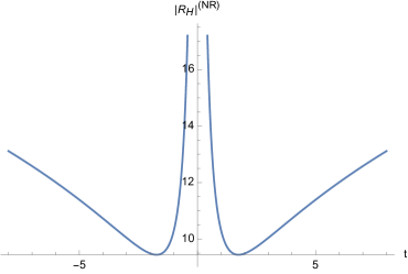
Figure 1: The absolute value of the comoving Hubble radius (6) for the nonrelativistic-matter solution and with $b=1$ and $t_{0}=4\sqrt{5}$. The suffix “NR” stands for “nonrelativistic” cosmological matter content.

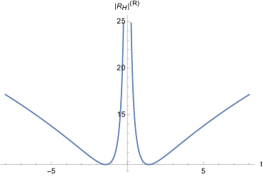
Figure 2: The absolute value of the comoving Hubble radius (6) for the relativistic-matter solution and with $b=1$ and $t_{0}=4\sqrt{5}$. The suffix “R” stands for “relativistic” cosmological matter content.

The plot of (the absolute value of) $R_{\rm H}(t)$ is displayed in Figs. 1 and 2. It is clear that the comoving Hubble radius diverges both at $t=0$ (which is a peculiar feature of all bouncing cosmologies) and, most importantly, at great distances from the defect. Therefore, the asymptotic behaviour of the comoving Hubble radius (6) is the same as the one predicted by those bouncing models characterized by primordial perturbation modes generated at very large negative cosmic times (see e.g. Nojiri et al. (2019)). The other viable picture occurs when $R_{\rm H}(t)$ vanishes asymptotically, resulting in perturbation modes produced near the bouncing epoch (see Ref. Odintsov et al. (2020) for further details).

In view of our forthcoming analysis, it will be crucial to define two different types of observers. First of all, we have the freely falling comoving observer known as the Eulerian observer. It is easy to show that for this observer, whose proper time will be indicated with $\tau$, the unit timelike four-velocity vector can be written as Misner et al. (1973)

$$\dfrac{{\rm d}x^{\alpha}}{{\rm d}\tau}\equiv n^{\alpha}=\dfrac{\sqrt{t^{2}+b^{2}}}{|t|}(1,0,0,0),$$ (7)

where we have introduced the usual notation $x^{\mu}=\left(t,x^{i}\right)$. It will soon be clear that the motion of the Eulerian observer is characterized by a vanishing conserved momentum $\Pi$ (see Eq. (10) below). We also note that Eq. (7) is not defined at $t=0$ (cf. Eq. (1d)). However, we will see that this fact will not prevent us from computing quantities we are interested in.

The second observer, which throughout the paper will be referred to as the “traveller”, is a generic freely falling non-comoving observer having a unit timelike four-velocity vector given by

$$\dfrac{{\rm d}x^{\alpha}}{{\rm d}\tau^{\prime}}\equiv v^{\alpha},$$ (8)

where $\tau^{\prime}$ denotes the traveller’s proper time. Due to the spatial maximal symmetry of (1a) and the associated conserved angular momentum, we will suppose that, without loss of generality, the traveller moves in the $(t,x)$-plane. Therefore, from the condition $\bm{v}\cdot\bm{v}=-1$ we obtain

$$\left(\dfrac{{\rm d}t}{{\rm d}\tau^{\prime}}\right)^{2}=\left(\dfrac{t^{2}+b^{2}}{t^{2}}\right)\left[1+a(t)^{2}\left(\dfrac{{\rm d}x}{{\rm d}\tau^{\prime}}\right)^{2}\right].$$ (9)

Furthermore, we can define the conserved momentum $\Pi$ along the traveller’s timelike geodesic as

$$\Pi=V^{(x)}_{\alpha}\dfrac{{\rm d}x^{\alpha}}{{\rm d}\tau^{\prime}}=a(t)^{2}\dfrac{{\rm d}x}{{\rm d}\tau^{\prime}},$$ (10)

$\bm{V}^{(x)}$ being the spacelike $x$-translational Killing vector. Therefore, the nonvanishing components of the traveller’s four velocity (8) read as

$$v^{t}=\sqrt{\left(\dfrac{t^{2}+b^{2}}{t^{2}}\right)\left(1+\dfrac{\Pi^{2}}{a(t)^{2}}\right)},$$ (11a)

$$v^{x}=\dfrac{\Pi}{a(t)^{2}}.$$ (11b)

Bearing in mind the above equations, if we consider a setup where the traveller moves along the increasing direction of the $x$-axis (i.e., $\Pi>0$ and ${\rm d}x/{\rm d}t>0$), then we can write the corresponding geodesic equation as

$$\dfrac{{\rm d}x(t)}{{\rm d}t}=\dfrac{|t|}{\sqrt{t^{2}+b^{2}}}\dfrac{1}{\sqrt{a(t)^{2}\left(1+a(t)^{2}/\Pi^{2}\right)}}.$$ (12)

We have solved Eq. (12) and have seen that the traveller’s timelike geodesics turn out to be well-behaved at $t=0$. This agrees with the analysis of null geodesics performed in Sec. IIIA of Ref. Klinkhamer and Wang (2019). However, it should be stressed that, since Levi-Civita connection of degenerate metrics is not unique, some ambiguities in the study of geodesic equation can arise (see Ref. Günther (September 2017) for further details).

3 Compressive forces acting on observers

In this section, we will evaluate the compressive forces felt by the Eulerian observer and the traveller as they travel towards the defect. In that regard, we will suppose to deal with human observers, meaning that we will assume that they are made of atoms.

In order to evaluate the abovementioned compressive forces, we will employ two different instantaneous rest frames: the proper reference frame $\mathbb{e}_{\hat{\alpha}}=(\mathbb{e}_{\hat{\tau}},\mathbb{e}_{\hat{x}},\mathbb{e}_{\hat{y}},\mathbb{e}_{\hat{z}})$ of the Eulerian observer and the proper reference frame $\mathbb{e}_{\hat{\alpha}^{\prime}}=(\mathbb{e}_{\hat{\tau}^{\prime}},\mathbb{e}_{\hat{x}^{\prime}},\mathbb{e}_{\hat{y}^{\prime}},\mathbb{e}_{\hat{z}^{\prime}})$ of the traveller. Such frames will be constructed in Eqs. (14)–(16) and (27) and (28), respectively. We are aware of the fact that in our model (1) the equivalence principle does not hold at $t=0$ and for this reason we will employ the limit $t\to 0$ to evaluate at $t=0$ the quantities we are interested in (details can be found in Ref. Günther (September 2017)).

The compressive forces felt by a (human) observer are measured via the components of the Riemann curvature tensor occurring in the geodesic deviation equation evaluated in his/her local orthonormal frame. We recall that the geodesic deviation equation can be written as Misner et al. (1973)

$$\Delta a^{\alpha}=-F^{\alpha}_{\rm compressive},$$ (13a)

$$F^{\alpha}_{\rm compressive}=R^{\alpha}_{\phantom{\alpha}\beta\gamma\delta}u^{\beta}\xi^{\gamma}u^{\delta},$$ (13b)

where $\Delta\bm{a}=\nabla_{\bm{u}}\nabla_{\bm{u}}\bm{\xi}$ is the relative acceleration of two freely falling test particles (i.e., two nearby geodesics) having separation vector $\bm{\xi}$ and four-velocity $\bm{u}$.

With the above premises, we are ready to construct the proper reference frame $\{\mathbb{e}_{\hat{\alpha}}\}$ of the Eulerian observer and to calculate compressive forces acting on him/her. We will see that we can get the traveller’s proper reference frame $\{\mathbb{e}_{\hat{\alpha}^{\prime}}\}$ by simply applying a Lorentz boost to Eulerian observer’s frame. Since both the Eulerian observers and the traveller are freely falling observers, their proper reference frames turn out to be local Lorentz frames all along their geodesics worldline (with the exclusion of $t=0$, i.e., the defect). The employed coordinates (which are Riemann normal coordinates with axes marked by gyroscopes, see Sec. 13.6 of Ref. Misner et al. (1973) and also Refs. Hartle (2003); Manasse and Misner (1963) for details) are know as Fermi normal coordinates (we have explicitly checked that the conditions $\nabla_{\bm{n}}\mathbb{e}_{\hat{\alpha}}=0$ and $\nabla_{\bm{v}}\mathbb{e}_{\hat{\alpha}^{\prime}}=0$ hold). By invoking the usual tetrad formalism Nakahara (2003) we obtain

$$\bm{g}=\eta_{\hat{\mu}\hat{\nu}}\,\bm{\theta}^{\hat{\mu}}\otimes\bm{\theta}^{\hat{\nu}},$$ (14a)

$$\bm{\theta}^{\hat{\tau}}=\sqrt{\dfrac{t^{2}}{t^{2}+b^{2}}}\,\mathbb{d}t,$$ (14b)

$$\bm{\theta}^{\hat{x}^{i}}=a(t)\,\mathbb{d}x^{i}.$$ (14c)

From the relations

$$\bm{\theta}^{\hat{\alpha}}=e^{\hat{\alpha}}_{\phantom{\hat{\alpha}}\mu}\,\mathbb{d}x^{\mu},$$ (15a)

$$e^{\hat{\alpha}}_{\phantom{\hat{\alpha}}\mu}e_{\hat{\beta}}^{{\phantom{\hat{\beta}}\mu}}=\delta^{\hat{\alpha}}_{\hat{\beta}},$$ (15b)

$$\mathbb{e}_{\hat{\alpha}}=e_{\hat{\alpha}}^{{\phantom{\hat{\alpha}}\mu}}\mathbb{e}_{\mu},$$ (15c)

we get (see Eq. (7))

$$\mathbb{e}_{\hat{\tau}}=\sqrt{\dfrac{t^{2}+b^{2}}{t^{2}}}\,\mathbb{e}_{t}=\bm{n},$$ (16a)

$$\mathbb{e}_{\hat{x}^{i}}=\dfrac{1}{a(t)}\mathbb{e}_{x^{i}}.$$ (16b)

The components $R_{\hat{\alpha}\hat{\beta}\hat{\gamma}\hat{\delta}}$ of the Riemann tensor in the proper reference frame $(\mathbb{e}_{\hat{\tau}},\mathbb{e}_{\hat{x}},\mathbb{e}_{\hat{y}},\mathbb{e}_{\hat{z}})$ can be obtained from those computed in the frame $\mathbb{e}_{\mu}=(\mathbb{e}_{t},\mathbb{e}_{x},\mathbb{e}_{y},\mathbb{e}_{z})$ through

$$R_{\hat{\alpha}\hat{\beta}\hat{\gamma}\hat{\delta}}=e_{\hat{\alpha}}^{\phantom{\hat{\alpha}}\alpha}e_{\hat{\beta}}^{\phantom{\hat{\beta}}\beta}e_{\hat{\gamma}}^{\phantom{\hat{\gamma}}\gamma}e_{\hat{\delta}}^{\phantom{\hat{\delta}}\delta}R_{\alpha\beta\gamma\delta},$$ (17a)

$$R^{\hat{\alpha}}_{\phantom{\hat{\alpha}}\hat{\beta}\hat{\gamma}\hat{\delta}}=\eta^{\hat{\alpha}\hat{\mu}}R_{\hat{\mu}\hat{\beta}\hat{\gamma}\hat{\delta}}.$$ (17b)

At this stage, we can analyze the compressive forces acting on the Eulerian human observer by evaluating the geodesic deviation equation in his/her proper reference. If we set $\bm{u}=\bm{n}$ in Eq. (13) and exploit Eqs. (16a) and (17) along with the condition $\bm{\xi}\cdot\bm{n}=-\xi^{\hat{\tau}}=0$, we obtain (no sum over $\hat{j}$):

$$\Delta a^{\hat{j}}=-R^{\hat{j}}_{\phantom{\hat{j}}\hat{\tau}\hat{j}\hat{\tau}}\,\xi^{\hat{j}},$$ (18a)

$$\Delta a^{\hat{j}}=\dfrac{{\rm d}^{2}}{{\rm d}\tau^{2}}\,\xi^{\hat{j}},$$ (18b)

$$-R^{\hat{j}}_{\phantom{\hat{j}}\hat{\tau}\hat{j}\hat{\tau}}=\left[\left(\dfrac{b^{2}+t^{2}}{t^{2}}\right)\dfrac{\ddot{a}}{a}+\left(-\dfrac{b^{2}}{t^{3}}\,\dfrac{\dot{a}}{a}\right)\right]\\ =\left\{\begin{array}[]{rl}&-\dfrac{2}{9\left(b^{2}+t^{2}\right)},\quad{\rm nonrelativistic\;matter},\\ &-\dfrac{1}{4\left(b^{2}+t^{2}\right)},\quad{\rm relativistic\;matter}.\end{array}\right.$$ (18c)

The fact that Eq. (18) depends on both first order and second order derivatives of $a(t)$ marks a difference with standard RW cosmology, which predicts compressive forces depending only on the ratio $\ddot{a}/a$. On the other hand, the minus sign occurring in front of the quantities contained inside the curly bracket in Eq. (18c) shows that we are dealing with compressive forces (cf. Eq. (13)), in strict analogy with standard RW cosmology Wald (1984), where Friedmann equations foretell a scale factor having $\ddot{a}<0$ as long as $\rho>0$ and $P\geq 0$ ($\rho$ and $P$ being, as pointed out in Sec. 2, the matter energy density and the matter pressure, respectively).

Equation (18c) implies that compressive forces acting at $t=0$ on the Eulerian human observer are given by

$$\begin{split}&\lim_{t\rightarrow 0}\left(-R_{\hat{x}\hat{\tau}\hat{x}\hat{\tau}}\right)=\lim_{t\rightarrow 0}\left(-R_{\hat{y}\hat{\tau}\hat{y}\hat{\tau}}\right)=\lim_{t\rightarrow 0}\left(-R_{\hat{z}\hat{\tau}\hat{z}\hat{\tau}}\right)\\ &=\left\{\begin{array}[]{rl}&-2/(9b^{2}),\quad{\rm nonrelativistic\;matter},\\ &-1/(4b^{2}),\quad{\rm relativistic\;matter},\end{array}\right.\end{split}$$ (19)

meaning that such observer is subjected to forces inversely proportional to the square of the length scale $b$ when he/she gets at the defect.

Let us analyze separately the two terms occurring in the square brackets of Eq. (18c). First of all, we have

$$\begin{split}\dfrac{\ddot{a}(t)}{a(t)}&=\left\{\begin{array}[]{rl}&\dfrac{2\left(3b^{2}-t^{2}\right)}{9\left(b^{2}+t^{2}\right)^{2}},\quad{\rm nonrelativistic\;matter},\\ &\dfrac{\left(2b^{2}-t^{2}\right)}{4\left(b^{2}+t^{2}\right)^{2}},\quad\,{\rm relativistic\;matter},\end{array}\right.\end{split}$$ (20)

which means that in a finite time interval around $t=0$ (i.e., near the defect) we have

$$\begin{split}\dfrac{\ddot{a}(t)}{a(t)}>0\Leftrightarrow&\left\{\begin{array}[]{rl}&-\sqrt{3}\,b<t<\sqrt{3}\,b,\quad\;{\rm nonrelativistic\;matter},\\ &-\sqrt{2}\,b<t<\sqrt{2}\,b,\quad\;{\rm relativistic\;matter}.\end{array}\right.\end{split}$$ (21)

Equations (20) and (21) imply that the factor $\ddot{a}/a$ occurring in Eq. (18c) produces stretching forces in the neighbourhood of the defect and compressive forces far from it. In particular, if we define

$$t^{\star}\equiv\sqrt{n}\,b,$$ (22a)

$$\begin{split}n=&\left\{\begin{array}[]{rl}&3,\quad{\rm nonrelativistic\;matter},\\ &2,\quad{\rm relativistic\;matter},\end{array}\right.\end{split}$$ (22b)

we can say that if $t<-t^{\star}$ (contracting-universe phase) or $t>t^{\star}$ (expanding-universe phase) the term $\ddot{a}/a$ generates a compressive force, whereas if $-t^{\star}<t<0$ (contracting epoch) or $0<t<t^{\star}$ (expanding epoch) $\ddot{a}/a$ leads to stretching forces. Here, we can appreciate the antigravitational action of the defect, which produces an accelerated contraction or expansion rate of the universe for $t\in\left(-t^{\star},t^{\star}\right)$.

The second term appearing in the square brackets of Eq. (18c) always causes compressive forces, since we have

$$\begin{split}-\dfrac{\dot{a}(t)}{a(t)}\dfrac{b^{2}}{t^{3}}&=\left\{\begin{array}[]{rl}&-\dfrac{2b^{2}}{3\left(b^{2}+t^{2}\right)},\quad{\rm nonrelativistic\;matter},\\ &-\dfrac{b^{2}}{2\left(b^{2}+t^{2}\right)},\quad{\rm relativistic\;matter}.\end{array}\right.\end{split}$$ (23)

However, we have already seen that the sum of the two contributions of Eq. (18c) amounts to a compressive force. This means that near the defect, where the terms $\ddot{a}/a$ and $[-(\dot{a}/a)(b^{2}/t^{3})]$ give opposite contributions, the modulus of $[-(\dot{a}/a)(b^{2}/t^{3})]$ “wins” against $\ddot{a}/a$ (which is positive for $-t^{\star}<t<t^{\star}$, cf. Eq. (21)) so that their sum gives a compressive force.

In principle, it could be possible to build a scenario where both compressive and stretching forces act on the Eulerian human observer in the vicinity of the defect. However, this would require, in the spacetime (1), a scale factor for which (at least) third-order time derivatives are nonvanishing at $t=0$. In other words, such a model would entail an odd $a(t)$ function.

For future purposes, it is important to express the components $R^{\hat{j}}_{\phantom{\hat{j}}\hat{\tau}\hat{j}\hat{\tau}}$ (no sum over $\hat{j}$) of the Riemann tensor appearing in Eq. (18) in an equivalent way. Indeed, the Riemann tensor written in terms of the Christoffel symbols $\Gamma^{\hat{\gamma}}_{\phantom{\hat{\gamma}}\hat{\alpha}\hat{\beta}}$ only reads as Nakahara (2003)

$$R^{\hat{\alpha}}_{\phantom{\hat{\alpha}}\hat{\beta}\hat{\gamma}\hat{\delta}}=\mathbb{e}_{\hat{\gamma}}\left[\Gamma^{\hat{\alpha}}_{\phantom{\hat{\alpha}}\hat{\delta}\hat{\beta}}\right]-\mathbb{e}_{\hat{\delta}}\left[\Gamma^{\hat{\alpha}}_{\phantom{\hat{\alpha}}\hat{\gamma}\hat{\beta}}\right]+\Gamma^{\hat{\epsilon}}_{\phantom{\hat{\epsilon}}\hat{\delta}\hat{\beta}}\Gamma^{\hat{\alpha}}_{\phantom{\hat{\alpha}}\hat{\gamma}\hat{\epsilon}}-\Gamma^{\hat{\epsilon}}_{\phantom{\hat{\epsilon}}\hat{\gamma}\hat{\beta}}\Gamma^{\hat{\alpha}}_{\phantom{\hat{\alpha}}\hat{\delta}\hat{\epsilon}}-\Gamma^{\hat{\alpha}}_{\phantom{\hat{\alpha}}\hat{\epsilon}\hat{\beta}}\left(\Gamma^{\hat{\epsilon}}_{\phantom{\hat{\epsilon}}\hat{\gamma}\hat{\delta}}-\Gamma^{\hat{\epsilon}}_{\phantom{\hat{\epsilon}}\hat{\delta}\hat{\gamma}}\right),$$ (24)

and the relation between the connection coefficients $\Gamma^{\hat{\gamma}}_{\phantom{\hat{\gamma}}\hat{\alpha}\hat{\beta}}$ in the basis $\{\mathbb{e}_{\hat{\alpha}}\}$ and $\Gamma^{\nu}_{\phantom{\nu}\mu\lambda}$ in the basis $\{\mathbb{e}_{\mu}\}$ is given by Nakahara (2003)

$$\Gamma^{\hat{\gamma}}_{\phantom{\hat{\gamma}}\hat{\alpha}\hat{\beta}}=e^{\hat{\gamma}}_{\phantom{\hat{\gamma}}\nu}e_{\hat{\alpha}}^{\phantom{\hat{\alpha}}\mu}\left(\partial_{\mu}e_{\hat{\beta}}^{\phantom{\hat{\beta}}\nu}+e_{\hat{\beta}}^{\phantom{\hat{\beta}}\lambda}\,\Gamma^{\nu}_{\phantom{\nu}\mu\lambda}\right).$$ (25)

Therefore, from Eqs. (24) and (25) we find

$$-R^{\hat{j}}_{\phantom{\hat{j}}\hat{\tau}\hat{j}\hat{\tau}}=\mathbb{e}_{\hat{\tau}}\left[\Gamma^{\hat{j}}_{\phantom{\hat{j}}\hat{j}\hat{\tau}}\right]+\left(\Gamma^{\hat{j}}_{\phantom{\hat{j}}\hat{j}\hat{\tau}}\right)^{2}=e_{\hat{\tau}}^{\phantom{\hat{\tau}}t}\,\mathbb{e}_{t}\left[e_{\hat{\tau}}^{\phantom{\hat{\tau}}t}\,\Gamma^{j}_{\phantom{j}jt}\right]+\left(e_{\hat{\tau}}^{\phantom{\hat{\tau}}t}\,\Gamma^{j}_{\phantom{j}jt}\right)^{2},\quad({\rm no\;sum\;over}\;\hat{j},j),$$ (26)

which, after having exploited Eqs. (14)–(16), leads to the same result as Eq. (18c).

The most important aspect of the above calculation is that Eq. (26) has no contribution from $\Gamma^{t}_{\phantom{t}tt}$ (i.e., the only Christoffel symbol of (1) which does not depend on $a(t)$ and its derivatives, see Eq. (4)). Indeed, this observation will be crucial in Sec. 4, where we will claim that compressive forces (18) show no substantial differences with respect to the corresponding standard cosmology case because the Eulerian observer cannot measure contributions related to $\Gamma^{t}_{\phantom{t}tt}$ in his/her proper reference frame (see the discussion below Eq. (62)).

At this stage, we are ready to move to the proper reference frame $(\mathbb{e}_{\hat{\tau}^{\prime}},\mathbb{e}_{\hat{x}^{\prime}},\mathbb{e}_{\hat{y}^{\prime}},\mathbb{e}_{\hat{z}^{\prime}})$ of the traveller by means of a boost along the $\mathbb{e}_{\hat{x}}$ direction. We can calculate the ordinary boost velocity $V^{\hat{x}}$ as

$$\begin{split}V^{\hat{x}}&=\dfrac{{\rm proper\,distance\,along\,}\mathbb{e}_{\hat{x}}\,{\rm as\,seen\,by\,the\,Eulerian\,observer}}{{\rm proper\,lapse\,time\,as\,seen\,by\,the\,Eulerian\,observer}}\\ &=\dfrac{\sqrt{g_{xx}}\,{\rm d}x}{\sqrt{-g_{tt}}\,{\rm d}t}=\dfrac{1}{\sqrt{1+a(t)^{2}/\Pi^{2}}}\equiv V,\end{split}$$ (27)

where we have exploited Eq. (11). In terms of the orthonormal bases $\{\mathbb{e}_{\hat{\alpha}}\}$ of the Eulerian observer and $\{\mathbb{e}_{\hat{\alpha}^{\prime}}\}$ of the traveller, the boost is expressed by

$$\left\{\begin{array}[]{rl}&\mathbb{e}_{\hat{\tau}^{\prime}}=\gamma\mathbb{e}_{\hat{\tau}}+\gamma V\mathbb{e}_{\hat{x}},\\ &\mathbb{e}_{\hat{x}^{\prime}}=\gamma V\mathbb{e}_{\hat{\tau}}+\gamma\mathbb{e}_{\hat{x}},\\ &\mathbb{e}_{\hat{y}^{\prime}}=\mathbb{e}_{\hat{y}},\\ &\mathbb{e}_{\hat{z}^{\prime}}=\mathbb{e}_{\hat{z}},\end{array}\right.$$ (28a)

$$\mathbb{e}_{\hat{\tau}^{\prime}}=\bm{v},$$ (28b)

$$\gamma=\dfrac{1}{\sqrt{1-V^{2}}}=\sqrt{1+\Pi^{2}/a(t)^{2}}.$$ (28c)

The components $R_{\hat{\alpha}^{\prime}\hat{\beta}^{\prime}\hat{\gamma}^{\prime}\hat{\delta}^{\prime}}$ of the Riemann tensor in the traveller’s proper frame can be obtained by applying the usual Lorentz transformation to the components $R_{\hat{\alpha}\hat{\beta}\hat{\gamma}\hat{\delta}}$ measured by the Eulerian observer in his/her proper frame. Moreover, since the separation vector $\bm{\xi}_{T}$ is purely spatial in the traveller’s frame, the geodesic deviation equation (13) can be written as

$$\Delta a^{\hat{i}^{\prime}}=\Delta a_{\hat{i}^{\prime}}=-R_{\hat{i}^{\prime}\hat{\tau}^{\prime}\hat{j}^{\prime}\hat{\tau}^{\prime}}\,\xi_{T}^{\hat{j}^{\prime}},$$ (29a)

$$\Delta a^{\hat{i}^{\prime}}=\dfrac{{\rm d}^{2}}{{\rm d}\tau^{\prime\,2}}\,\xi_{T}^{\hat{i}^{\prime}}.$$ (29b)

Bearing in mind the above equation, the compressive forces felt by the human traveller as he/she passes through the defect are given by

$$\lim_{t\rightarrow 0}\left(-R_{\hat{x}^{\prime}\hat{\tau}^{\prime}\hat{x}^{\prime}\hat{\tau}^{\prime}}\right)=\left\{\begin{array}[]{rl}&-2/(9b^{2}),\quad{\rm nonrelativistic\;matter},\\ &-1/(4b^{2}),\quad{\rm relativistic\;matter},\end{array}\right.$$ (30a)

$$\begin{split}&\lim_{t\rightarrow 0}\left(-R_{\hat{y}^{\prime}\hat{\tau}^{\prime}\hat{y}^{\prime}\hat{\tau}^{\prime}}\right)=\lim_{t\rightarrow 0}\left(-R_{\hat{z}^{\prime}\hat{\tau}^{\prime}\hat{z}^{\prime}\hat{\tau}^{\prime}}\right)=\\ &\left\{\begin{array}[]{rl}&-[2/(9b^{2})](1+3\Pi^{2}/a(0)^{2}),\quad\quad{\rm nonrelativistic\;matter},\\ &-[1/(4b^{2})](1+2\Pi^{2}/a(0)^{2}),\quad\quad{\rm relativistic\;matter}.\end{array}\right.\end{split}$$ (30b)

At this stage, if we take into account the hypothesis developed in Ref. Klinkhamer (2020a) according to which the defect length scale $b$ can be of order of the Planck length ${\ell}_{\rm P}$ and we also suppose that

$$t_{0}\gg b,$$ (31a)

$$\dfrac{|\Pi|t_{0}}{b}\gg 1,$$ (31b)

we can write (30b) approximately as

$$\begin{split}&\lim_{t\rightarrow 0}\left(-R_{\hat{y}^{\prime}\hat{\tau}^{\prime}\hat{y}^{\prime}\hat{\tau}^{\prime}}\right)=\lim_{t\rightarrow 0}\left(-R_{\hat{z}^{\prime}\hat{\tau}^{\prime}\hat{z}^{\prime}\hat{\tau}^{\prime}}\right)\approx\\ &\left\{\begin{array}[]{rl}&-[2\Pi^{2}(t_{0})^{4/3}]/[3b^{2}(b)^{4/3}],\quad\;{\rm nonrelativistic\;matter},\\ &-[\Pi^{2}\,|t_{0}|\,]/[2b^{3}],\quad\quad\quad\quad\quad\,{\rm relativistic\;matter}.\end{array}\right.\end{split}$$ (32)

Some comments on the results obtained so far are in order. First of all, Eqs. (19) and (30) show that compressive forces are finite at $t=0$ provided that $b\neq 0$. This may be seen as an equivalent proof of the fact that in the RW geometry (1) the big-bang singularity can be regularized via the introduction of the defect Klinkhamer (2019). Furthermore, the analysis of compressive forces acting on both the Eulerian observer and the traveller reveals that the spacetime defect can be identified as the three-dimensional spacelike hypersurface of the regularized RW spacetime where compressive forces become as intense as possible. This is clear from Fig. 3, where we have chosen to plot compressive forces experienced by the Eulerian observer in the case of nonrelativistic-matter solution (cf. Eq. (3)). Compressive forces on the Eulerian observer for the relativistic-matter solution and on the traveller (for both the matter-dominated and the radiation-dominated universe) display the same behaviour as the one in Fig. 3.

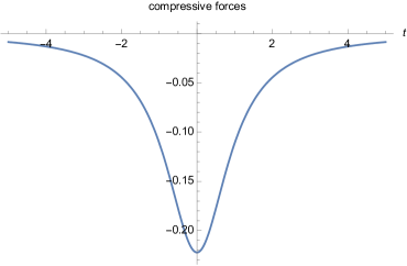
Figure 3: Compressive forces acting on the Eulerian observer for the nonrelativistic-matter solution (3) and with $b=1$ (cf. Eq. (18c)). A similar plot is obtained for compressive forces experienced by the traveller.

Moreover, Eqs. (19), (30) and (32) show that if $b\sim{\ell}_{\rm P}$ then both the Eulerian human observer and the human traveller are subjected to very large compressive forces proportional to $1/b$ as they pass the defect, which therefore amounts to a gravitational obstacle between two different universes, the one with $t<0$ and that with $t>0$. To have an idea, a rough calculation reveals that if we assume that a human body cannot withstand an acceleration gradient of ten times the Earth’s gravity (i.e., $10g_{\oplus}\approx 98$ m/s²) per metre, then Eq. (19) implies that the Eulerian human observer can survive the compressive forces generated at $t=0$ only if $b\gtrsim 10^{7}$ m. This suggests that the results of this section can concur with the analysis performed in Refs. Klinkhamer (2020a); Klinkhamer and Wang (2020); Klinkhamer (2020c) (see also Ref. Klinkhamer (2021, to appear in Acta Phys. Polon. B)) where a quantum origin of the defect length scale is proposed. Indeed, as spelled out in Ref. Klinkhamer (2021, to appear in Acta Phys. Polon. B), our model (1) could yield two possible scenarios, depending on the values assumed by the defect length scale $b$. The first pattern leads to a nonsingular-bouncing-cosmology model, whereas the second provides a new physics phase at $t=0$ which pair-produces a “universe” for $t>0$ and an “anti-universe” for $t<0$. The first framework is built on classical Einstein theory and hence may be possible if $b\gg{\ell}_{\rm P}$, whereas the second might apply if $b\sim{\ell}_{\rm P}$. Our investigation shares some similar features with this last situation since we have shown that if $b\sim{\ell}_{\rm P}$ then compressive forces become so large at $t=0$ that the universe having $t<0$ and the one with $t>0$ can be viewed as separated.

It should be stressed that Eqs. (18) and (29) (likewise those derivable thereof) will not hold exactly, since they do not account for the forces between the atoms comprising the observers. Nevertheless, when gravitational compressive forces become very strong such interatomic forces can be neglected and hence the equations derived above will be valid to good approximation. Therefore, we can conclude that when compressive forces tear the Eulerian human observer and the human traveller apart, the very atoms of which they are composed must ultimately undergo the same fate.

4 The energy of massive particles and photons

We have examined, in the previous section, compressive forces acting on the Eulerian human observer and the human traveller. In order to complete our physical description of the spacetime defect underlying the modified RW cosmology (1), we will now analyze the energy behaviour of both the Eulerian observer and the traveller during their motion. Furthermore, our investigation will involve the energy of photons. We also note that for these considerations we have no need to think of the Eulerian observer and the traveller as human observers.

First of all, we need to define the concept of massive particle or photon energy in a proper way. Before we set out this theme, let us describe two simple situations where we can safely define this physical quantity. As a first example, consider the Schwarzschild solution. In this case, it is possible to define the total energy of a massive particle or a photon due to the presence of a timelike Killing vector field related to the time-translation invariance of Schwarzschild geometry; moreover, in the case of timelike geodesics, this conserved quantity reduces, at large distances from the center of attraction, to the usual special relativistic formula for the total energy per unit mass of the particle Wald (1984). Another example is furnished by the energy of a massive particle or a photon with four-momentum $\bm{p}$ which is (locally) measured by a generic observer having four-velocity $\bm{u}_{\rm obs}$ in his/her proper reference frame (whose orthonormal basis four-vectors are such that $\mathbb{e}_{\hat{0}}=\bm{u}_{\rm obs}$). In this case, we find

$$E_{\rm measured}=-\bm{p}\cdot\bm{u}_{\rm obs}=p^{\hat{0}}=\langle\bm{\theta}^{\hat{0}},\bm{p}\rangle,$$ (33)

where $\{\bm{\theta}^{\hat{\alpha}}\}$ is the basis one-forms of the observer’s proper reference frame (cf. Eq. (14a)) and $\langle\cdot\,,\,\cdot\rangle$ is the usual inner product. However, in this case thre is a caveat: expression (33) only represents an intrinsic energy from motion and inertia, not the total energy of the massive particle or the photon. In that regard, we will see that in our model Eq. (33) yields, in agreement with the equivalence principle (which holds for all times except at $t=0$), an expression for the energy measured by the Eulerian observer where there is no room for the term $\Gamma^{t}_{\phantom{t}tt}$, which, as we have pointed out in Sec. 3, fulfils an important role in our analysis. Indeed, we will interpret this $\Gamma^{t}_{\phantom{t}tt}$ term as due to the (anti-)gravitational action of the defect (see comments above Eq. (54)).

To formulate an energy definition suitable for our model, we need to briefly recall some topics. It is well-known that the Hamiltonian formulation of general relativity as well as the analysis of the Cauchy (initial value) problem can be performed by employing the $3+1$ formalism, which relies on a theorem stating that any globally hyperbolic spacetime can be foliated by a constant-$t$ family $(\Sigma_{t})_{t\in\mathbb{R}}$ of spacelike (Cauchy) hypersurfaces Wald (1984); Gourgoulhon (2012); Choquet-Bruhat (2014); Hawking and Ellis (1973). Within this framework, the spacetime metric can be written as

$$g_{\mu\nu}=\begin{bmatrix}N_{i}N^{i}-N^{2}&N_{k}\\ N_{k}&h_{ik}\end{bmatrix},$$ (34)

where $N$, $N_{i}$ are the lapse function and the shift vector, respectively, while $h_{ik}$ is the (induced) 3-metric on the generic hypersurface $\Sigma_{t}$ belonging to the set $(\Sigma_{t})_{t\in\mathbb{R}}$. An inspection of Eq. (1a), reveals that in our model we have

$$N=\dfrac{|t|}{\sqrt{t^{2}+b^{2}}},$$ (35a)

$$N_{i}=0,$$ (35b)

$$h_{ik}=a(t)^{2}\delta_{ik}.$$ (35c)

Furthermore, in the context of the geometry of foliation the Eulerian observer four-velocity can be written in general as $n^{\alpha}=(\dfrac{1}{N},\dfrac{-N^{i}}{N})$ and it represents the timelike and future-oriented unit four-vector normal to the generic hypersurface $\Sigma_{t}$. In our modified RW setup, it follows from Eqs. (35a) and (35b) that Eq. (7) can be written equivalently as

$$n^{\alpha}=\dfrac{1}{N}(1,0,0,0).$$ (36)

An important object of the $3+1$ approach is the so-called normal evolution (four-)vector Gourgoulhon (2012), defined as the timelike vector field

$$\bm{m}\equiv N\bm{n},$$ (37)

which carries (or Lie drags) the hypersurface $\Sigma_{t}$ (defined, as pointed out before, by the condition $t={\rm const}$) to the neighbouring hypersurface $\Sigma_{t+{\rm d}t}$. In other words, the hypersurface $\Sigma_{t+{\rm d}t}$ can be obtained from the neighbouring $\Sigma_{t}$ by a small displacement $\bm{m}\,{\rm d}t$ of each point of $\Sigma_{t}$. From Eq. (36) we easily find that our regularized RW geometry is characterized by the following normal evolution (four-)vector:

$$\bm{m}=\mathbb{e}_{t}.$$ (38)

Bearing in mind the above results, we propose for model (1) the following definition of the total energy. We identify the total energy $E_{\rm tot}$ of a massive particle or a photon having four-momentum $\bm{p}$ with the projection of $\bm{p}$ along the normal evolution (four-)vector, i.e.,

$$E_{\rm tot}=-\bm{p}\cdot\bm{m}.$$ (39)

This is justified by the fact that, as explained before, the four-vector $\bm{m}$ regulates the temporal evolution of the spacetime (note however that this evolution is described in terms of the coordinate time variable $t$, see below). Therefore, the procedure underlying Eq. (39) turns out to be similar to the method adopted by an observer who measures the (intrinsic) energy of a massive particle/photon in his/her proper reference frame by simply projecting the massive particle/photon four-momentum $\bm{p}$ along $\mathbb{e}_{\hat{0}}=\bm{u}_{\rm obs}$, i.e., along the time direction defined by the observer’s clock (cf. Eq. (33)). In a similar way, we propose through Eq. (39) to define the total energy by projecting $\bm{p}$ along the four-vector $\bm{m}$ ruling the evolution of the spacetime. We will justify later in which sense (39) defines a total energy (see comments below Eq. (54)). However, in our definition (39) there is one important aspect which must be taken into account: while $\mathbb{e}_{\hat{0}}$ governs the flow of the observer’s proper time, $\bm{m}$ can be seen as the vector controlling the flow of the coordinate time.

We can analyze the consequences of our definition (39) by considering the form assumed by $E_{\rm tot}$ in the most general situations. Consider for instance the generic four-dimensional spacetime metric written as in Eq. (34). According to our definition (39), the total energy $\mathcal{E}$ of the Eulerian observer is given by (for the sake of simplicity, the rest masses of all observers are set to one)

$$\mathcal{E}=-\bm{n}\cdot\bm{m}=N=-n_{t}.$$ (40)

Now consider a generic particle having four-momentum $\bm{p}$. According to our prescription (39), the total energy will be

$$E_{\rm particle}=-\bm{p}\cdot\bm{m}=N^{2}p^{t}.$$ (41)

In this case, $E_{\rm particle}\neq-p_{t}$ since

$$-p_{t}=N^{2}p^{t}-N_{i}N^{i}p^{t}-N_{i}p^{i},$$ (42)

and hence

$$E_{\rm particle}=-p_{t}\Leftrightarrow N^{i}=0.$$ (43)

Equations (41)–(43) reveal the advantages of our definition (39). Indeed, Eq. (41) depends only on the gauge function $N$ (reflecting thus the fact that the energy is not a scalar and hence its expression changes according to the coordinates adopted), whereas (42) depends on both $N$ and $N^{i}$. However, this last circumstance would lead to an ill-defined concept of energy since the contributions due to $N^{i}$ can always be gauged away once comoving spatial coordinates are invoked. On the contrary, by adopting the definition (41), the energy does not depend on terms which can be set to zero by an appropriate coordinate transformation.

In model (1), the normal evolution (four-)vector is represented by Eq. (38) and hence we can define the total energy of the traveller and the photon as, respectively,

$$E=-\bm{v}\cdot\bm{m}=-v_{t},$$ (44a)

$$E_{\rm ph}=-\bm{k}\cdot\bm{m}=-k_{t},$$ (44b)

$\bm{k}$ being the photon four momentum. In addition, the total energy of the Eulerian observer will be represented by (40), which by means of Eq. (35a) reads as

$$\mathcal{E}=\sqrt{\dfrac{t^{2}}{t^{2}+b^{2}}}.$$ (45)

Let $E_{\rm local}$ represent the traveller energy as measured by the Eulerian observer in his/her proper reference frame $(\mathbb{e}_{\hat{\tau}},\mathbb{e}_{\hat{x}},\mathbb{e}_{\hat{y}},\mathbb{e}_{\hat{z}})$. Then we have from Eq. (33)

$$E_{\rm local}=-\bm{v}\cdot\bm{n}=-v_{\hat{\tau}}=v^{\hat{\tau}}=\langle\bm{\theta}^{\hat{\tau}},\bm{v}\rangle=\langle\bm{\theta}^{\hat{\tau}},v^{\nu}\mathbb{e}_{\nu}\rangle=\sqrt{-g_{tt}}\,\dfrac{{\rm d}t}{{\rm d}\tau^{\prime}}=\sqrt{1+\Pi^{2}/a(t)^{2}}=\gamma,$$ (46)

where we have exploited the well-known relation $\langle\mathbb{d}x^{\mu},\mathbb{e}_{\nu}\rangle=\delta^{\mu}_{\nu}$ and Eqs. (11a), (14b) and (28c). Similarly, the photon energy $E_{\rm ph,local}$ measured by the Eulerian observer in his/her proper reference frame is given by

$$E_{\rm ph,local}=-\bm{k}\cdot\bm{n}=-k_{\hat{\tau}}=k^{\hat{\tau}}=\sqrt{-g_{tt}}\,\dfrac{{\rm d}t}{{\rm d}s}=\dfrac{|\Pi_{\rm ph}|}{a(t)},$$ (47)

$s$ being the affine parameter along the photon’s null geodesics and $\Pi_{\rm ph}\equiv a(t)^{2}{\rm d}x/{\rm d}s$ the conserved momentum. Therefore, the total energy of the traveller and the photon reads as, respectively,

$$E=-v_{t}=\sqrt{-g_{tt}}\,E_{\rm local}=\sqrt{\dfrac{t^{2}}{t^{2}+b^{2}}}\left(\sqrt{1+\Pi^{2}/a(t)^{2}}\right),$$ (48a)

$$E_{\rm ph}=-k_{t}=\sqrt{-g_{tt}}\,E_{\rm ph,local}=\sqrt{\dfrac{t^{2}}{t^{2}+b^{2}}}\left(\dfrac{|\Pi_{\rm ph}|}{a(t)}\right).$$ (48b)

Equations (46)–(48) show that even if we reject our proposal of defining the total energy according to Eq. (39), we can at least say that the total energy $E$ of the traveller and the total energy $E_{\rm ph}$ of the photon make sense at great distances from the defect (i.e., if $|t|\gg b$), where they reduce to $E_{\rm local}$ and $E_{\rm ph,local}$, respectively. This is due to the fact that for large values of $t$ the lapse function (35a) is such that $N\to 1$, meaning that there is no difference between the Eulerian velocity $\bm{n}$ and the normal evolution (four-)vector $\bm{m}$ if $|t|\gg b$ (cf. Eqs. (36)–(38)). Therefore, we can write

$$E=-\bm{v}\cdot\bm{m}\xrightarrow[|t|\gg b]{}-\bm{v}\cdot\bm{n}=E_{\rm local},$$ (49a)

$$E_{\rm ph}=-\bm{k}\cdot\bm{m}\xrightarrow[|t|\gg b]{}-\bm{k}\cdot\bm{n}=E_{\rm ph,local}.$$ (49b)

The geodesic equation provides us with the equations governing the dynamical evolution of $E$ and $E_{\rm ph}$. After an easy calculation, we obtain

$$\dot{E}+\dfrac{\dot{a}}{a}E-\dfrac{\dot{a}}{a}\dfrac{1}{E}\left(\dfrac{t^{2}}{b^{2}+t^{2}}\right)=\Gamma^{t}_{\phantom{t}tt}E,$$ (50a)

$$\dot{E}_{\rm ph}+\dfrac{\dot{a}}{a}E_{\rm ph}=\Gamma^{t}_{\phantom{t}tt}E_{\rm ph}.$$ (50b)

A comparison with standard RW cosmology allows us to derive the equations ruling the dynamical behaviour of $E_{\rm local}$ and $E_{\rm ph,local}$, i.e.,

$$\dot{E}_{\rm local}+\dfrac{\dot{a}}{a}E_{\rm local}-\dfrac{\dot{a}}{a}\dfrac{1}{E_{\rm local}}=0,$$ (51a)

$$\dot{E}_{\rm ph,local}+\dfrac{\dot{a}}{a}E_{\rm ph,local}=0.$$ (51b)

The main difference between Eqs. (50) and (51) stems from the presence on the right hand side of the former of the connection coefficient $\Gamma^{t}_{\phantom{t}tt}$. As anticipated before, we will interpret this term as due to the (anti-)gravitational action generated by the defect. Furthermore, we note in Eqs. (50a) and (51a) a contribution proportional to the inverse of the energy originating from the nonvanishing magnitude of traveller’s four-velocity $\bm{v}$ via the condition $\bm{v}\cdot\bm{v}=-1$.

The plots of the traveller energy $E$ and the photon energy $E_{\rm ph}$ are shown in Figs. 4–7.

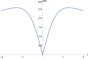
Figure 4: The traveller energy (48a) for the nonrelativistic-matter solution (3) and with $\Pi=1$, $b=1$, $t_{0}=4\sqrt{5}$. The suffix “NR” stands for “nonrelativistic” cosmological matter content.

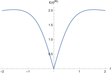
Figure 5: The traveller energy (48a) for the relativistic-matter solution (3) and with $\Pi=1$, $b=1$, $t_{0}=4\sqrt{5}$. The suffix “R” stands for “relativistic” cosmological matter content.

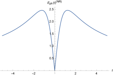
Figure 6: The photon energy (48b) for the nonrelativistic-matter solution (3) and with $\Pi_{\rm ph}=1$, $b=1$, $t_{0}=4\sqrt{5}$. The suffix “NR” stands for “nonrelativistic” cosmological matter content.

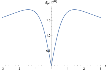
Figure 7: The photon energy (48b) for the relativistic-matter solution (3) and with $\Pi_{\rm ph}=1$, $b=1$, $t_{0}=4\sqrt{5}$. The suffix “R” stands for “relativistic” cosmological matter content.

From Figs. 4 and 5, it is clear that: in the negative-$t$ branch, the total energy of the traveller (48a) starts decreasing after a time interval during which it has increased; for $t>0$ we have the mirrored behaviour with respect to $t<0$; for $t=0$ the energy vanishes and $\lim\limits_{t\to\pm\infty}E=1$ (corresponding to the traveller’s rest mass). Moreover, apart from $t=0$, the energy (48a) is always positive. The traveller energy has thus a usual (i.e., standard) behaviour only away from the defect, where it increases (resp. decreases) while the universe contracts (resp. expands); on the contrary, near the defect the energy diminishes (resp. grows) as the universe undergoes a contracting (resp. expanding) era.

Something similar happens for the photon energy (48b), as Figs. 6 and 7 witness. In this case, $E_{\rm ph}$ is always positive except for $t=0$ and for large values of $|t|$, where it vanishes. In addition, the simple form assumed by Eq. (48b) permits to evaluate readily the sign of the time derivative $\dot{E}_{\rm ph}$. Indeed we find that (see Eq. (22))

$$\dot{E}_{\rm ph}>0\Leftrightarrow t<-\tilde{t}\;\;\cup\;\;0<t<\tilde{t},$$ (52a)

$$\tilde{t}\equiv\left\{\begin{array}[]{rl}&t^{\star}/\sqrt{2},\quad\quad{\rm nonrelativistic\;matter},\\ &t^{\star},\quad\quad\quad\quad{\rm relativistic\;matter}.\end{array}\right.$$ (52b)

Following Eq. (52), we see that the photon energy (48b) increases when $t<-\tilde{t}$ or $0<t<\tilde{t}$ and decreases if $-\tilde{t}<t<0$ or $t>\tilde{t}$. Thus, as for the traveller energy, $E_{\rm ph}$ has the usual behaviour only for $|t|\gg b$.

From the above analysis it is thus clear that the unusual character of the total energies $E$ and $E_{\rm ph}$ is due to the (anti-)gravitational action exerted by the defect through the term $\Gamma^{t}_{\phantom{t}tt}$, as Eq. (50) shows. Furthermore, the same nonstandard behaviour affects also the Eulerian observer energy $\mathcal{E}$ being, as it is clear from Eq. (45), monotonically decreasing for $t<0$ and monotonically increasing for $t>0$ (indeed the shape of the energy function $\mathcal{E}$ resembles the traveller energy displayed in Figs. 4 and 5).

We also note that we can interpret as a discontinuity in the (instantaneous) power the discontinuity of first kind that the total energy of the Eulerian observer, the traveller and the photon, Eqs. (45) and (48), shows at at $t=0$ (see Figs. 4–7).

At this stage, we can consider the traveller energy $E_{\rm local}$ and the photon energy $E_{\rm ph,local}$ as measured by the Eulerian observer in his/her proper reference frame $(\mathbb{e}_{\hat{\tau}},\mathbb{e}_{\hat{x}},\mathbb{e}_{\hat{y}},\mathbb{e}_{\hat{z}})$ (see Eqs. (46) and (47)). Their plots are shown in Figs. 8 and 9 and Figs. 10 and 11, respectively. It is thus clear that the energies (46) and (47) have always the usual character since, as we will show below, no contribution from $\Gamma^{t}_{\phantom{t}tt}$ can be measured by the Eulerian observer in his/her proper reference frame (however, a first clear evidence is given by Eq. (51)).

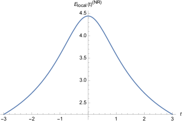
Figure 8: The traveller energy (46) for the nonrelativistic-matter solution (3) and with $\Pi=1$, $b=1$, $t_{0}=4\sqrt{5}$. It is clear that the maximum is reached at $t=0$. The suffix “NR” stands for “nonrelativistic” cosmological matter content.

Figure 9: The traveller energy (46) for the relativistic-matter solution (3) and with $\Pi=1$, $b=1$, $t_{0}=4\sqrt{5}$. It is clear that the maximum is attained when $t=0$. The suffix “R” stands for “relativistic” cosmological matter content.

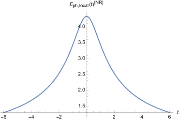
Figure 10: The photon energy (47) for the nonrelativistic-matter solution (3) and with $\Pi_{\rm ph}=1$, $b=1$, $t_{0}=4\sqrt{5}$. It is clear that the maximum is reached at $t=0$. The suffix “NR” stands for “nonrelativistic” cosmological matter content.

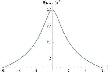
Figure 11: The photon energy (47) for the relativistic-matter solution (3) and with $\Pi_{\rm ph}=1$, $b=1$, $t_{0}=4\sqrt{5}$. It is clear that the maximum is reached at $t=0$. The suffix “R” stands for “relativistic” cosmological matter content.

By employing hypotheses (31), we have that

$$\lim_{t\rightarrow 0}E_{\rm local}=\sqrt{1+\Pi^{2}/a(0)^{2}}\approx\left\{\begin{array}[]{rl}&|\Pi|(t_{0}^{2})^{1/3}/(b^{2})^{1/3},\quad\quad\quad\quad\quad{\rm nonrelativistic\;matter},\\ &|\Pi|(t_{0}^{2})^{1/4}/(b^{2})^{1/4},\quad\quad\quad\quad\quad{\rm relativistic\;matter},\end{array}\right.$$ (53)

and hence it is clear that, at $t=0$, $E_{\rm local}$ is proportional to a fractional power of $1/b^{2}$ (see Figs. 8 and 9). This signifies an enormous amount of energy, if we suppose that $b$ is proportional to the Planck length $\ell_{\rm P}$. The same conclusions as those expressed by Eq. (53) hold also for the photon energy $E_{\rm ph,local}$ if we enforce (31a).

We have already seen (cf. Eq. (49)) that for large values of $t$ the total energies $E$ and $E_{\rm ph}$ reduce to the corresponding local intrinsic quantities $E_{\rm local}$ and $E_{\rm p,local}$, respectively. At this stage, we can provide a further explanation of this point. If we first consider the case of photon energy, we can see that if $|t|\gg b$ then, from Eq. (4), $\Gamma^{t}_{\phantom{t}tt}$ tends to zero and hence Eq. (50b) reduces to (51b), whose solution is represented by (47). The same holds also for the traveller energy, where in addition the term occurring in Eq. (50a), i.e.,

$$\dfrac{t^{2}}{t^{2}+b^{2}},$$

tends to one for large times and hence we can recover (51a), which in turn yields the expression (46).

As pointed out before, we can interpret $\Gamma^{t}_{\phantom{t}tt}$ as the term embodying the (anti-)gravitational action exerted by the defect. At this stage, we can account for this assumption. First of all, we have already explained that $\Gamma^{t}_{\phantom{t}tt}$ fulfils an important role in the equations governing the dynamical evolution of the total energy of the traveller and the photon (cf. Eq. (50)). Moreover, the fact that $\Gamma^{t}_{\phantom{t}tt}$ gets closer to zero if $|t|\gg b$ reflects that the action of the defect phases out as a particle travels away from it. Furthermore, $\Gamma^{t}_{\phantom{t}tt}$ diverges if $t\to 0$: the closer a particle gets to the defect, the stronger is the “force” it experiences. Moreover, it is possible to write $\Gamma^{t}_{\phantom{t}tt}$ as (cf. Eq. (4))

$$\Gamma^{t}_{\phantom{t}tt}=-\dfrac{1}{t}\dfrac{\rho_{\rm defect}}{\rho},$$ (54)

where (see Eq. (2.4c) in Ref. Klinkhamer and Wang (2020))

$$\rho_{\rm defect}\equiv-\dfrac{b^{2}\rho}{b^{2}+t^{2}}.$$ (55)

This means that the (anti-)gravitational “force” produced by the defect depends on the ratio between the effective energy density $\rho_{\rm defect}$ of the defect and the energy density $\rho$ of matter (or equivalently the ratio between their masses) as well as the inverse time separation from the defect.

The above analysis indicates also that $E$ and $E_{\rm ph}$ can be regarded as total energies since they take into account also the contribution due to $\Gamma^{t}_{\phantom{t}tt}$, unlike the intrinsic quantities $E_{\rm local}$ and $E_{\rm ph,local}$. Indeed, once $\Gamma^{t}_{\phantom{t}tt}$ vanishes, the energy will not contain the contributions coming from the gravitational action of the defect but it will include only those terms connected to the kinetic energy and the inertia. As a consequence, when $|t|\gg b$ the total energies reduce to the corresponding intrinsic expressions, as we have just demonstrated.

We have already seen that the proper reference frame of the Eulerian observer is a freely falling frame whose coordinates amount to be Fermi normal coordinates. In such a frame, the (Fermi normal) coordinates $x^{\hat{\mu}}$ of a generic point $\mathcal{P}$ located near the Eulerian observer’s worldline are given by

$$x^{\hat{\mu}}\left(\mathcal{P}\right)=\left(x^{\hat{\tau}},x^{\hat{j}}\right)=\left(\tau,s\,r^{\hat{j}}\right),$$ (56)

where $\bm{r}=r^{\hat{j}}\mathbb{e}_{\hat{j}}$ is the tangent vector to the (spacelike) geodesic originating from the Eulerian observer’s worldline at the specific (Eulerian observer’s) proper time $\tau$ and $s$ the proper length along such geodesic. If we employ the notation $f(x^{\hat{\tau}}=\tau,x^{\hat{j}}=0)\equiv\left.f\right|_{\mathcal{G}}$ to indicate that a quantity is evaluated along the Eulerian observer’s geodesic, we know from Ref. Manasse and Misner (1963) that Christoffel symbols satisfy the following relations:

$$\left.\partial_{\hat{\tau}}\Gamma^{\hat{\alpha}}_{\phantom{\hat{\alpha}}\hat{\mu}\hat{\nu}}\right|_{\mathcal{G}}=0,$$ (57a)

$$\left.\partial_{\hat{\nu}}\Gamma^{\hat{\alpha}}_{\phantom{\hat{\alpha}}\hat{\mu}\hat{\tau}}\right|_{\mathcal{G}}=\left.R^{\hat{\alpha}}_{\phantom{\hat{\alpha}}\hat{\mu}\hat{\nu}\hat{\tau}}\right|_{\mathcal{G}},$$ (57b)

$$\left.\partial_{\hat{k}}\Gamma^{\hat{\alpha}}_{\phantom{\hat{\alpha}}\hat{i}\hat{j}}\right|_{\mathcal{G}}=-\dfrac{1}{3}\left(\left.R^{\hat{\alpha}}_{\phantom{\hat{\alpha}}\hat{i}\hat{j}\hat{k}}\right|_{\mathcal{G}}+\left.R^{\hat{\alpha}}_{\phantom{\hat{\alpha}}\hat{j}\hat{i}\hat{k}}\right|_{\mathcal{G}}\right),$$ (57c)

from which we derive the following expansion for the Christoffel symbols:

$$\Gamma^{\hat{\alpha}}_{\phantom{\hat{\alpha}}\hat{\mu}\hat{\nu}}\left(\tau,x^{\hat{j}}\right)=\left.\partial_{\hat{k}}\Gamma^{\hat{\alpha}}_{\phantom{\hat{\alpha}}\hat{\mu}\hat{\nu}}\right|_{\mathcal{G}}x^{\hat{k}}+{\rm O}\left(|x^{\hat{k}}|^{2}\right).$$ (58)

From the above equation, we obtain the following relation, valid for our modified RW model:

$$\Gamma^{\hat{\tau}}_{\phantom{\hat{\tau}}\hat{\tau}\hat{\tau}}\left(\tau,x^{\hat{j}}\right)={\rm O}\left(|x^{\hat{k}}|^{2}\right).$$ (59)

This means that the connection coefficient $\Gamma^{\hat{\tau}}_{\phantom{\hat{\tau}}\hat{\tau}\hat{\tau}}$ vanishes not only along the geodesic $\mathcal{G}$ of the Eulerian observer but also in the neighbourhood of $\mathcal{G}$ (within the precision of ${\rm O}(|x^{\hat{k}}|)$). Accordingly, the energies $E_{\rm local}$ and $E_{\rm ph,local}$ measured by the Eulerian observer in his/her proper reference frame will not include the effects coming from $\Gamma^{\hat{\tau}}_{\phantom{\hat{\tau}}\hat{\tau}\hat{\tau}}$. This offers another explanation of the fact that, once the underlying computations are performed in the coordinate system $(t,x,y,z)$, the dynamical evolution of $E_{\rm local}$ and $E_{\rm ph,local}$ are ruled by Eq. (51), where no contribution from $\Gamma^{t}_{\phantom{t}tt}$ appears. In other words, the Eulerian observer will not take into account the gravitational action of the defect (represented, as we said before, by $\Gamma^{t}_{\phantom{t}tt}$) when he/she measures the energy of the photon or the massive particle.

We can also explain this point with a more direct approach. We know that, in Fermi normal coordinates, the geodesic equation can be written as

$$\dfrac{{\rm d^{2}}x^{\hat{\mu}}}{{\rm d}\lambda^{2}}+\Gamma^{\hat{\mu}}_{\phantom{\hat{\mu}}\hat{\nu}\hat{\alpha}}\left(\tau,x^{\hat{j}}\right)\dfrac{{\rm d}x^{\hat{\nu}}}{{\rm d}\lambda}\dfrac{{\rm d}x^{\hat{\alpha}}}{{\rm d}\lambda}=0,$$ (60)

where $\lambda$ is the affine parameter along the geodesic (which in the case of timelike geodesic can be identified with the particle’s proper time). Therefore, the energy $p^{\hat{\tau}}$ of a massive particle or a photon having four-momentum $p^{\hat{\alpha}}={\rm d}x^{\hat{\alpha}}/{\rm d}\lambda$ as measured by the Eulerian observer will obey the equation (we simply write $\Gamma^{\hat{\tau}}_{\phantom{\hat{\tau}}\hat{\nu}\hat{\alpha}}(\tau,x^{\hat{j}})\equiv\Gamma^{\hat{\tau}}_{\phantom{\hat{\tau}}\hat{\nu}\hat{\alpha}}$ in order to ease the notation)

$$\dfrac{{\rm d}p^{\hat{\tau}}}{{\rm d}\lambda}+\Gamma^{\hat{\tau}}_{\phantom{\hat{\tau}}\hat{\alpha}\hat{\beta}}p^{\hat{\alpha}}p^{\hat{\beta}}=0.$$ (61)

Bearing in mind Eqs. (14)–(16) and (25), we find that the coefficients $\Gamma^{\hat{\tau}}_{\phantom{\hat{\tau}}\hat{\alpha}\hat{\beta}}$ occurring in Eq. (61) are given by

$$\Gamma^{\hat{\tau}}_{\phantom{\hat{\tau}}\hat{\tau}\hat{\tau}}=\partial_{t}e_{\hat{\tau}}^{\phantom{\hat{\tau}}t}+e_{\hat{\tau}}^{\phantom{\hat{\tau}}t}\Gamma^{t}_{\phantom{t}tt}=0,$$ (62a)

$$\Gamma^{\hat{\tau}}_{\phantom{\hat{\tau}}\hat{\tau}\hat{i}}=e_{\hat{i}}^{\phantom{\hat{i}}j}\Gamma^{t}_{\phantom{t}tj}=0,$$ (62b)

$$\Gamma^{\hat{\tau}}_{\phantom{\hat{\tau}}\hat{i}\hat{\tau}}=e^{\hat{\tau}}_{\phantom{\hat{\tau}}t}e_{\hat{i}}^{\phantom{\hat{i}}i}\left(\partial_{i}e_{\hat{\tau}}^{\phantom{\hat{\tau}}t}+e_{\hat{\tau}}^{\phantom{\hat{\tau}}t}\Gamma^{t}_{\phantom{t}ti}\right)=0,$$ (62c)

$$\Gamma^{\hat{\tau}}_{\phantom{\hat{\tau}}\hat{i}\hat{j}}=e^{\hat{\tau}}_{\phantom{\hat{\tau}}t}e_{\hat{i}}^{\phantom{\hat{i}}i}e_{\hat{j}}^{\phantom{\hat{j}}j}\Gamma^{t}_{\phantom{t}ij}=\sqrt{\dfrac{b^{2}+t^{2}}{t^{2}}}\dfrac{\dot{a}(t)}{a(t)}\delta_{\hat{i}\hat{j}}.$$ (62d)

By means of Eq. (62), we can show that Eq. (61) reduces to Eq. (51) once all calculations are performed in $(t,x,y,z)$ coordinates. However, the most important point of this computation is that Eq. (62) clearly shows that $\Gamma^{\hat{\tau}}_{\phantom{\hat{\tau}}\hat{\tau}\hat{\tau}}$ is the only connection coefficient occurring in Eq. (61) which depends on $\Gamma^{t}_{\phantom{t}tt}$. Since $\Gamma^{\hat{\tau}}_{\phantom{\hat{\tau}}\hat{\tau}\hat{\tau}}$ vanishes, no contribution from $\Gamma^{t}_{\phantom{t}tt}$ appears in (51). As a result, the Eulerian observer will not measure the effects related to $\Gamma^{t}_{\phantom{t}tt}$, i.e., those contributions we are interpreting as due to the (anti-)gravitational action of the defect.

At this stage, let us stress another point. We have seen in Sec. 3 that compressive forces felt by the Eulerian (human) observer show no deviations from the expectations of standard cosmology. It is now clear that this result is due to the fact that the effects introduced by $\Gamma^{t}_{\phantom{t}tt}$ cannot be measured in the freely falling frame $(\mathbb{e}_{\hat{\tau}},\mathbb{e}_{\hat{x}},\mathbb{e}_{\hat{y}},\mathbb{e}_{\hat{z}})$, see Eq. (26) and comments below. Bearing in mind the previous analysis regarding the local energies (46) and (47), this means that physical quantities measured by the Eulerian observer do not display an unusual behaviour because in the proper reference frame $(\mathbb{e}_{\hat{\tau}},\mathbb{e}_{\hat{x}},\mathbb{e}_{\hat{y}},\mathbb{e}_{\hat{z}})$ no contribution from $\Gamma^{t}_{\phantom{t}tt}$ can appear.

In our analysis a final question must be answered. For the sake of clarity, in the following calculations we will keep the observers’ rest mass explicit. Accordingly, let $\mu_{\rm E}$ denote the Eulerian observer’s rest mass. We know that comoving coordinates $(t,x,y,z)$ introduced in Eqs. (1d) and (1e) allow for the description of the modified model of universe from the point of view of the Eulerian observer. Recalling that such observer is always at rest in these coordinates, we are thus led to wonder about the reasons for which our definition (39) of total energy leads to Eq. (40) instead of an expression like $\mathcal{E}=\mu_{\rm E}$. The answer is that (39) defines a total energy and hence it takes into account also the defect’s gravitational action. This means that the total energy of the Eulerian observer (40) (or equivalently (45)) receives a contribution from the defect such that $\mathcal{E}\neq\mu_{\rm E}$. Indeed, we simply have

$$\mathcal{E}=-\mu_{\rm E}\left(\bm{n}\cdot\bm{m}\right)=\mu_{\rm E}\sqrt{\dfrac{t^{2}}{t^{2}+b^{2}}}=\sqrt{\mu_{\rm E}^{2}+\mu_{\rm E}^{2}\dfrac{\rho_{\rm{defect}}}{\rho}}.$$ (63)

In other words, $\mathcal{E}$ differs from $\mu_{\rm E}$ by a term involving the ratio $\rho_{\rm defect}/\rho$, i.e., the same term occurring in the expression of $\Gamma^{t}_{\phantom{t}tt}$ (see Eq. (54)). Therefore, the presence of the defect makes $\mathcal{E}$ differ from the Eulerian observer’s rest mass $\mu_{\rm E}$. Similarly, the total energy of the traveller (48a) can be written as

$$E=-\mu_{\rm T}\left(\bm{v}\cdot\bm{m}\right)=\sqrt{\mu_{\rm T}^{2}+\mu_{\rm T}^{2}\dfrac{\rho_{\rm{defect}}}{\rho}}\sqrt{1+\dfrac{\Pi^{2}}{a(t)^{2}}},$$ (64)

$\mu_{\rm T}$ being the traveller’s rest mass. In this expression we can recognize both the defect’s gravitational action, represented by the term $\mu_{\rm T}\rho_{\rm defect}/\rho$ and the “kinetic” term proportional to $\Pi^{2}/a(t)^{2}$. Finally, the photon energy (48b) reads as

$$E_{\rm ph}=\sqrt{1+\dfrac{\rho_{\rm defect}}{\rho}}\,\dfrac{|\Pi_{\rm ph}|}{a(t)}.$$ (65)

In this case, we can interpret the “correction” term $\rho_{\rm defect}/\rho$ as a photon’s effective mass induced by the defect.

Equations (63)–(65) support, once again, our proposal of interpreting (39) as the total energy of a massive particle/photon with four-momentum $\bm{p}$. On the other hand, (33) denotes an intrinsic energy which does not take into account the defect’s gravitational force, represented by the term $\Gamma^{t}_{\phantom{t}tt}$. Indeed, in Eqs. (63)–(65) the term $\rho_{\rm defect}/\rho$, originating from $\Gamma^{t}_{\phantom{t}tt}$, appears explicitly. On the contrary, in Eqs. (46) and (47) no contribution coming from $\Gamma^{t}_{\phantom{t}tt}$ can occur, as we have explained before (cf. Eq. (51) and comments following Eqs. (59) and (62)).

5 Conclusions and open problems

The main purpose of this paper consists in seeking physical observables which can point out the presence of the spacetime defect characterizing the regularized RW geometry (1), where the big-bang singularity has been tamed by a nonzero length parameter $b$. Our description relies on the analysis of two physical quantities: the compressive forces acting on (human) observers and the energy of massive particles and photons crossing it. The first topic has been explored in Sec. 3. We have devised a reasonable criterion to single out the defect, which can be defined as the three-dimensional hypersurface where the modulus of compressive forces attain their maximum value (see Fig. 3). Furthermore, we have found that if we take the proposal $b\sim{\ell}_{\rm P}$ made in Appendix B of Ref. Klinkhamer (2020a) seriously, then the defect can be modelled as a gravitational obstacle with compressive forces proportional to $1/b$ (see Eqs. (19), (30) and (32)). A rough calculation reveals that a Eulerian human observer can withstand compressive forces generated at $t=0$ if $b\gtrsim 10^{7}$ m. This result can lead to interesting implications due to the possibility of having a quantum-inspired defect length scale. In particular, we have explained how our investigation seems to agree with the scenario drawn in Ref. Klinkhamer (2021, to appear in Acta Phys. Polon. B) suggesting that a new physics phase at $t=0$ could create a pair of separated universes.

In Sec. 4, we have provided a definition of a total energy suitable for our model (see comments accompanying Eqs. (39) and (49)) which differentiates it from the (local) intrinsic energy measured by the Eulerian observer (see comments below Eqs. (54) and (65)). We have seen that both the total energy of the generic freely falling observer and of the photon, defined according to (39) and given in Eq. (48), exhibit an unusual character over a finite time interval around $t=0$: they grow (resp. diminish) as the universe expands (resp. contracts); see Figs. 4–7. As an inspection of Eq. (50) reveals, this scenario is due to the effects introduced by the Christoffel symbol $\Gamma^{t}_{\phantom{t}tt}$ (cf. Eq. (4)), which we propose to interpret as the term embodying the (anti-)gravitational action exerted by the defect (see comments below Fig. 11). Furthermore, the same nonstandard behaviour affects also the Eulerian observer energy (45). On the other hand, the intrinsic energy of the generic freely falling traveller and of the photon, given in Eqs. (46) and (47), respectively, displays no unusual property (see Figs. 8–11 and comments therein). This absence of discrepancy with respect to standard cosmology predictions stems from the fact that the Eulerian observer cannot measure contributions related to the Christoffel symbol $\Gamma^{t}_{\phantom{t}tt}$ in his/her proper reference frame (see comments following Eqs. (59) and (62)).

A possible explanation of the nonstandard behaviour of the energy can come from the following hypothesis involving gravitationally repulsive negative masses. A negative mass is an exotic matter which would violate one or more energy conditions. It can be implemented in general relativity theory Bondi (1957), where the equivalence principle implies that the inertial mass equals the passive gravitational mass. Consider the situation depicted in Fig. 12, where, for simplicity, the gravitational positive-negative mass interaction is explored by means of Newtonian theory and the negative mass is supposed to be fixed. The gravitational repulsive force $\vec{F}_{g}$ experienced by the moving body and the resulting acceleration $\vec{a}$ point along the same direction. In panel (a), the positive mass approaches with velocity $\vec{v}$ the negative mass. Since the work done by $\vec{F}_{g}$ is negative, the positive mass slows down. In panel (b), the positive mass departs from the fixed body. In this case, it is clear that the kinetic energy of the moving body increases. Furthermore, the mechanical energy is conserved in both situations. This classical example can give us some insight into the nature of the defect. First of all, recall that in a generic spacetime there will not be a well-defined notion of gravitational potential energy (although in special cases it exists). In our relativistic model, if we conceive the defect as an object having negative (active gravitational) mass, then it is possible to account for the behaviour of the energy as shown in Figs. 4–7. Indeed, over a small time interval around the bounce, where anti-gravitational phenomena reveal an increasing importance, the energy of both massive particles and photons decreases for negative values of the time variable $t$ and grows when $t$ becomes positive. This reflects the behaviour of the kinetic energy in the classical example of Fig. 12. Moreover, at great distances from the defect, the energy displays its standard behaviour, meaning that antigravitational effects are negligible (as witnessed by the fact that $\Gamma^{t}_{\phantom{t}tt}$ goes to zero if $|t|\gg b$, see Eq. (4)). Furthermore, this scenario allows for the fact that the energy drops to zero at $t=0$: the defect drains the energy of particles until, at the bounce, it vanishes; after that, the defect gives to particles the required energy to carry on with their motion. Therefore, we can conclude that the effective NEC violation featuring the defect and the related antigravity effects represent the source of the nonstandard behaviour of the total energy shown in Figs. 4–7. Incidentally, the possibility of modelling the defect as an object having negative mass has been discussed also in Ref. Klinkhamer and Queiruga (2018). This hypothesis can open interesting prospectives. As an example, recently in Ref. Farnes (2018) gravitationally repulsive negative masses have been proposed as natural candidates for the description of both dark matter and dark energy. Thus, we might wonder if also the defect can represent such candidate.

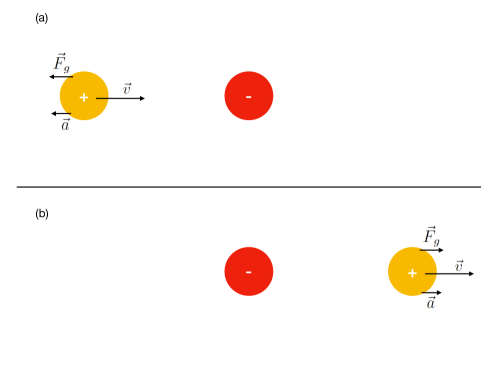
Figure 12: Gravitational repulsion experienced by a positive (yellow) mass due to the presence of a body with negative (red) mass, which is supposed to be fixed. The interaction is described through Newtonian theory. (a) The positive mass goes toward the fixed body with velocity $\vec{v}$; (b) the positive mass moves away from the fixed body with velocity $\vec{v}$. In both cases, the gravitational repulsive force $\vec{F}_{g}$ and the resulting acceleration $\vec{a}$ have the same direction and point away from the negative mass.

The analysis of Sec. 4 has shown that the nonstandard properties of massive particles and photons energy are not confined to the single point $t=0$, but they concern a finite time interval around the defect’s location which is of the order of the characteristic length scale $b$. This pattern is in accordance with the aforementioned proposed interpretation of the connection coefficient $\Gamma^{t}_{\phantom{t}tt}$ since, as we have explained in the comments above Eq. (54), this function attains large values in a region around $t=0$ (except for $t=0$, where it is not defined) and approaches zero as $|t|\gg b$. This means that the unusual energy’s behaviour configures as a sort of “spreading effect” able to encompass regions near the defect. This is not the first example of a “spreading effect” occurring in the modified RW geometry (1), the other one being represented by the effective NEC violation which, as reported in Refs. Klinkhamer (2020a); Klinkhamer and Wang (2020), can be extended to a finite interval around $t=0$. Therefore, these results lead quite naturally to one important (open) question: are there other “spreading phenomena” in nonsingular-bouncing-cosmology settings?

Another fascinating issue to be addressed, especially in light of the outcome of this paper, regards the origin of the defect length scale $b$. Indeed, if its quantum origin were proven, then an intriguing task would consists in trying to reconcile this fact with the arguments spelled out in our paper. On the other hand, a broader investigation is performed in Ref. Klinkhamer (2020c), where it is argued that $b$ could be a remnant of a new (not necessarily quantum) physics phase replacing Einstein gravity (see also Ref. Klinkhamer (2021, to appear in Acta Phys. Polon. B)). It would be interesting to determine if there exists a connection between the physical effects discussed in this paper and the new phase mentioned in Ref. Klinkhamer (2020c).

Finally, the rich mathematical structure underlying regularized RW geometry (1) (likewise degenerate metrics in general, see Ref. Günther (September 2017)) still deserves further investigation. Indeed, this can represent, on the one hand, a way to find other physical phenomena associated with the defect, and, on the other, we can expect to obtain equivalent explanations for the physical effects described in this paper.

References

- Klinkhamer (2019) F. R. Klinkhamer, “Regularized big bang singularity,” Phys. Rev. D 100, 023536 (2019), arXiv:1903.10450 .
- Klinkhamer (2020a) F. R. Klinkhamer, “More on the regularized big bang singularity,” Phys. Rev. D 101, 064029 (2020a), arXiv:1907.06547 .
- Klinkhamer and Wang (2019) F. R. Klinkhamer and Z. L. Wang, “Nonsingular bouncing cosmology from general relativity,” Phys. Rev. D 100, 083534 (2019), arXiv:1904.09961 .
- Klinkhamer and Wang (2020) F. R. Klinkhamer and Z. L. Wang, “Nonsingular bouncing cosmology from general relativity: Scalar metric perturbations,” Phys. Rev. D 101, 064061 (2020), arXiv:1911.06173 .
- Klinkhamer (2020b) F. R. Klinkhamer, “Another model for the regularized big bang,” (2020b), arXiv:2005.12157 .
- Ashtekar (2009) A. Ashtekar, “Loop Quantum Cosmology: An Overview,” Gen. Rel. Grav. 41, 707–741 (2009), arXiv:0812.0177 .
- Lidsey et al. (2000) J. E. Lidsey, D. Wands, and E. J. Copeland, “Superstring cosmology,” Phys. Rept. 337, 343–492 (2000), arXiv:9909061 .
- Klinkhamer (2020c) F. R. Klinkhamer, “IIB matrix model and regularized big bang,” PTEP 2021, 063 (2020c), arXiv:2009.06525 .
- Klinkhamer (2021) F. R. Klinkhamer, “IIB matrix model: Emergent spacetime from the master field,” PTEP 2021, 013B04 (2021), arXiv:2007.08485 .
- Klinkhamer (2021, to appear in Acta Phys. Polon. B) F. R. Klinkhamer, “M-theory and the birth of the Universe,” in 27th Cracow Epiphany Conference on Future of particle physics (2021, to appear in Acta Phys. Polon. B) arXiv:2102.11202 .
- Becker et al. (2006) K. Becker, M. Becker, and J. H. Schwarz, String theory and M-theory: A modern introduction (Cambridge University Press, 2006).
- Günther (September 2017) M. Günther, Skyrmion spacetime defect, degenerate metric, and negative gravitational mass (Master Thesis, KIT, Karlsruhe, September 2017).
- Wald (1984) R. M. Wald, General relativity (Chicago University Press, Chicago, 1984).
- Misner et al. (1973) C. W. Misner, K. S. Thorne, and J. A. Wheeler, Gravitation (W. H. Freeman, San Francisco, 1973).
- Akrami et al. (2020) Y. Akrami et al. (Planck), “Planck 2018 results. X. Constraints on inflation,” Astron. Astrophys. 641, A10 (2020), arXiv:1807.06211 .
- Nojiri et al. (2019) Shin’ichi Nojiri, S. D. Odintsov, V. K. Oikonomou, and Tanmoy Paul, “Nonsingular bounce cosmology from Lagrange multiplier gravity,” Phys. Rev. D 100, 084056 (2019), arXiv:1910.03546 .
- Elizalde et al. (2020) E. Elizalde, S. D. Odintsov, V. K. Oikonomou, and Tanmoy Paul, “Extended matter bounce scenario in ghost free gravity compatible with GW170817,” Nucl. Phys. B 954, 114984 (2020), arXiv:2003.04264 .
- Odintsov et al. (2020) S. D. Odintsov, V. K. Oikonomou, and Tanmoy Paul, “From a Bounce to the Dark Energy Era with Gravity,” Class. Quant. Grav. 37, 235005 (2020), arXiv:2009.09947 .
- Belinsky et al. (1970) V. A. Belinsky, I. M. Khalatnikov, and E. M. Lifshitz, “Oscillatory approach to a singular point in the relativistic cosmology,” Adv. Phys. 19, 525–573 (1970).
- Bunch and Davies (1978) T. S. Bunch and P. C. W. Davies, “Quantum Field Theory in de Sitter Space: Renormalization by Point Splitting,” Proc. Roy. Soc. Lond. A 360, 117–134 (1978).
- Birrell and Davies (1984) N. D. Birrell and P. C. W. Davies, Quantum Fields in Curved Space, Cambridge Monographs on Mathematical Physics (Cambridge Univ. Press, Cambridge, 1984).
- Hartle (2003) J. B. Hartle, Gravity: An Introduction to Einstein’s General Relativity (Addison-Wesley, San Francisco, 2003).
- Manasse and Misner (1963) F. K. Manasse and C. W. Misner, “Fermi normal coordinates and some basic concepts in differential geometry,” Journal of Mathematical Physics 4, 735–745 (1963).
- Nakahara (2003) M. Nakahara, Geometry, topology and physics, Graduate student series in physics (Hilger, Bristol, 2003).
- Gourgoulhon (2012) E. Gourgoulhon, 3+1 Formalism in General Relativity: Bases of Numerical Relativity, Lecture Notes in Physics (Springer, Berlin, 2012).
- Choquet-Bruhat (2014) Y. Choquet-Bruhat, Introduction to General Relativity, Black Holes, and Cosmology (Oxford University Press, Oxford, 2014).
- Hawking and Ellis (1973) S. W. Hawking and G. F. R. Ellis, The Large Scale Structure of Space-Time, Cambridge Monographs on Mathematical Physics (Cambridge University Press, Cambridge, 1973).
- Bondi (1957) H. Bondi, “Negative Mass in General Relativity,” Rev. Mod. Phys. 29, 423–428 (1957).
- Klinkhamer and Queiruga (2018) F. R. Klinkhamer and J. M. Queiruga, “Antigravity from a spacetime defect,” Phys. Rev. D 97, 124047 (2018), arXiv:1803.09736 .
- Farnes (2018) J. S. Farnes, “A unifying theory of dark energy and dark matter: Negative masses and matter creation within a modified CDM framework,” Astron. Astrophys. 620, A92 (2018), arXiv:1712.07962 .