Controlling Photoluminescence Spectra of hBN Color Centers by Selective Phonon-Assisted Excitation: A Theoretical Proposal
Abstract
Color centers in hexagonal boron nitride (hBN) show stable single photon emission even at room temperature, making these systems a promising candidate for quantum information applications. Besides this remarkable property, also their interaction with longitudinal optical (LO) phonons is quite unique because they lead to dominant phonon sidebands (PSBs), well separated from the zero phonon line (ZPL). In this work we utilize this clear spectral separation to theoretically investigate the influence of phonon decay dynamics on time-dependent photoluminescence (PL) signals. Our simulations show, that by using tailored optical excitation schemes it is possible to create a superposition between the two LO modes, leading to a phonon quantum beat that manifests in the time-dependent PL signal.
Accepted manuscript for publication in Materials for Quantum Technology (CC BY 4.0).
https://doi.org/10.1088/2633-4356/abcbeb
1 Introduction
A few years ago the family of solid state single photon emitters (SPEs) was joined by a promising new group in the form of color centers in hexagonal boron nitride (hBN) [1]. These systems show single photon emission even at room temperature [1, 2, 3, 4, 5]. Despite rapid intense investigations the exact atomic structure is still under debate [1, 3, 6, 7, 8, 9, 10]. However a few candidates have been identified to likely contain carbon [6, 7, 11]. Beyond its characterization, recent studies have focused on the coherent optical control [12] and the manipulation of spin states with external magnetic fields [9, 13].
All solid state SPEs unavoidably interact with lattice distortions and therefore couple to phonons [14, 15]. In this context many former studies have focused on minimizing the impact of the phonon coupling on SPEs [16, 17]. This could in principle be possible in hBN color centers by reducing the dipole moment of the emitter wave function [18]. Here, we follow a different approach by making direct use of this interaction to control the emitter by tailored phonon-assisted excitations.
The coupling between phonons and the hBN-SPEs has some unique properties, compared to other emitters, like semiconductor quantum dots (QDs) or NV centers in diamond. In QDs the exciton-phonon interaction is rather weak, leading to emission spectra that are dominated by the zero phonon line (ZPL) [19, 20, 21, 22, 23]. The QD excitons couple predominantly to acoustic phonons [21], which often render a limiting factor to coherent control [22, 16, 24, 23]. In NV centers in diamond the optical response is dominated by phonon sidebands (PSBs) which mainly stem from local mode oscillations with energies of a few ten meVs [25, 26, 27]. Especially at room temperature the PSBs strongly overlap and make a separation from the ZPL challenging [28, 29]. Compared to these two types of SPEs the phonon coupling of hBN color centers is quite unique. Because of the strong polarity of the hBN crystal and the color centers therein coupling to longitudinal optical (LO) modes is remarkably strong. It results in peaks that are well separated from the ZPL by approximately 200 meV and that can reach heights of up to half the ZPL [18].
It has been shown that optical excitation of SPEs via phonon-assisted processes is very efficient. While in QDs typically excitation via acoustic PSBs is chosen [30, 31, 32], in hBN the LO-PSBs provide an efficient excitation channel [18, 33]. This makes these modes excellent candidates to investigate the underlying interplay with the color center in more detail and study the influence of phonon dynamics. So far only equilibrium spectra of color centers in hBN have been studied in detail in the literature [5, 18, 34]. Here, we go a step further and simulate time-dependent photoluminescence (PL) spectroscopy signals. We model an actual experimental realization of this dynamically and spectrally resolved PL measurement. There we focus on the phonons’ effect on non-equilibrium dynamics of PL spectra after a pulsed laser excitation. In practice we study the thermalization process and quantum beats of the LO phonons. This is a first important step towards more advanced quantum state preparation of the phonons by tailored optical excitation schemes of the color center [35, 36, 37].
2 Theory
In this work we calculate time-dependent PL spectra of a hBN color center after a phonon-assisted excitation with a short laser pulse. The color center inevitably interacts with the LO phonons of the host lattice. Further dephasing and decay of the emitter, as well as decay of the LO modes due to anharmonicities, are accounted for by Lindblad dissipators.
2.1 The model
For the states of the hBN color center we assume a two-level system (TLS) consisting of a ground state and an excited state . Although some studies suggest additional dark states that lie below the optically active one [1, 4, 38], we restrict our model to the TLS for the following reasons. It was shown that this approach allows to reproduce optical spectra [18] and we are here only interested in (sub-)picosecond dynamics, which is much faster than typical transitions involving the dark states [38].
In Ref. [18] it was shown that the independent boson model is suitable to calculate absorption spectra of single color centers. Therefore we start with the Hamiltonian [39, 21]
| (1) | |||||
where is the transition operator from the excited to the ground state with an energy splitting that is typically in the optical range. is the frequency of the -th phonon mode with annihilation and creation operators and , respectively. The coupling constants are given by , where the index collectively denotes all quantum numbers, that are used to label the phonon modes, i.e., branch index and momentum. Low energy phonons like acoustic and local modes are hard to separate from the ZPL contribution at room temperature because of their significant spectral overlap. But the LO modes in hBN have energies of up to 200 meV, which makes them easy to isolate spectrally even at room temperature. For simplicity we assume dispersionless LO branches, which already led to excellent results in Ref. [18]. In this case, we can describe a single LO branch by a single collective boson mode [40].
The coupling of the emitter to the electrical field of a laser pulse is described within the usual dipole and rotating wave approximation via the interaction Hamiltonian
| (2a) | |||||
| where the effective laser field reads | |||||
| (2b) | |||||
and and are the dipole operator and the real envelope of the electrical field of the laser pulse, respectively. We choose the effective laser field to be a Gaussian pulse with temporal width , centered around time , with the dimensionless pulse area .
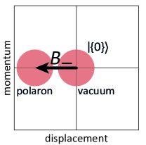
The full unitary dynamics of the system is described by the Hamiltonian . In absence of the laser field, the Hamiltonian reduces to , which can be diagonalized by the so-called polaron transformation [39, 41, 42, 43]. With this transformation one can find the eigenstates of to be
| (2ca) | |||
| where is an arbitrary multi-mode Fock state and | |||
| (2cb) | |||
are multi-mode displacement operators, displacing each phonon mode by in phase space. We see that the ground state of the phonon subsystem is the multi-mode vacuum , in the case that the TLS is in the ground state . However for the case, that it is in the excited state , the ground state for the phonon subsystem is the displaced vacuum . As schematically depicted in Fig. 1 this simply describes that, induced by an excitation of the TLS, the lattice relaxes to a new equilibrium position forming the so-called polaron [44, 45]. It also leads to a renormalization of the transition energy by the polaron-shift to . Consequently also the coupling to the laser field is renormalized, such that the pulse area changes as , where is the expectation value of with respect to the initial thermal phonon state [46, 43]. Note, that is the same for and because it is just given by the overlap between the displaced and the original thermal distribution in phase space. Therefore it is independent of the direction of the displacement.
2.2 Dissipation
We describe the non-unitary dynamics of the system by a set of Lindblad dissipators, i.e., we restrict ourselves to Markovian dynamics [47]. Decay and pure dephasing of the TLS are described by the dissipators [48]
| (2cda) | |||
| and | |||
| (2cdb) | |||
respectively, acting on the density matrix . Here, is the excited state decay time, i.e., the lifetime of the emitter and the additional pure dephasing time. Note that the decay automatically includes a dephasing time . It is known that the lifetime of the hBN emitters is in the nanosecond range independent of temperature while the detected dephasing time is much shorter. Therefore the additional pure dephasing has to be considered here.
We will later focus on the dynamics of the high energy LO modes. For these modes two aspects are important: (A) Due to their energies way above 100 meV they are thermally unoccupied even at room temperature and (B) they typically have lifetimes of a few ps [49]. To account for (B) we use a dissipator, describing the decay of a single LO mode with the rate , given by
| (2cde) | |||||
The dissipator from Eq. (2cde) consists of three parts: describes the relaxation of the mode LOj to its vacuum, in the case that the emitter is in the ground state . is more involved and describes the relaxation into the displaced vacuum , i.e., the polaron configuration, when the emitter is in the excited state . does not lend itself to such an easy interpretation, but we see that it only acts on the polarization of the TLS, i.e., density matrix elements proportional to or , leaving the state of the TLS unchanged. As discussed in the next section, the PL spectrum is determined only by the occupation of the TLS, i.e., density matrix elements proportional to , apart from the time during the laser pulse interaction. Since the laser pulse duration that is chosen in this work is fs, much shorter than typical values of the LO phonon lifetime [49], this part of the dissipator is of minor importance. This has been checked by comparing numerical calculations of spectra with and without . The derivation of Eq. (2cde) is given in the Supplementary Material (SM). Finally, the Lindblad equation that governs the dynamics of the system is given by
2.3 Time-dependent spectroscopy
To model time-dependent PL spectra, we consider a filter, e.g. a Fabry-Perot interferometer, that selects the light emitted from the hBN defect, before the intensity of the filtered light field is detected as a function of time. The spectral width of the filter will at the same time yield a finite temporal resolution due to time-energy uncertainty. The time-dependent PL spectrum of the emitter, using a filter with a Lorentzian spectrum, is given by [50, 51]
| (2cdg) | |||||
A short derivation of this formula is given in the SM. We see, that the spectral width of the spectrometer leads to a finite spectral resolution, due to its appearance in the -integration. At the same time it appears as a finite integration time over the history of the system up until time , which results in the finite time resolution mentioned before. Consequently, a perfect spectral and temporal resolution cannot be achieved at the same time. By integrating Eq. (2cdg) over the time , we obtain the (time-integrated) PL spectrum of the emitter. The central quantity to determine the time-dependent PL spectrum is the causal two-time correlation function of the TLS. We will calculate this quantity numerically, applying the quantum regression theorem, together with Eq. (2.2) [47]. The regression theorem can be applied here because the dynamics of our TLS+LO phonon system is described by a Lindblad equation and is therefore Markovian (see SM for more details). We perform the calculations in a truncated Hilbert space limiting the maximum number of phonons per mode. An important property of this correlation function is that, if and are times after the interaction with the laser pulse, only the part of the density matrix proportional to contributes to the PL signal, since does not lead to any transitions in the TLS. This is true even in the presence of the dissipators in Eq. (2.2), as discussed in the SM. Thus, the subspace of the system, in which the state is occupied, entirely determines the spectrum, apart from contributions during the laser pulse interaction.
3 Results
Before coming to the characteristic two–LO-mode structure of hBN color centers we simplify the system and consider just a single LO mode. This reduced model allows us to instructively explain the influence of a phonon-assisted excitation and the decay of the LO phonon mode on the PL signal dynamics. We furthermore neglect the influence of low energy phonons like acoustic modes. Therefore we will not get an asymmetric broadening of the ZPL and additional broadenings of the PSBs. However, since all phonon modes couple independently to the TLS, this will not influence the dynamics induced by the LO modes significantly. Due to the possible LO energies between meV and meV [18] we can safely assume the thermal equilibrium state for these modes to be the vacuum state even at room temperature.
In the following we choose the ZPL energy to be eV. While the lifetime of the emitter ns is considered to be independent of the temperature, the dephasing time changes with temperature and we choose fs at 300 K, fs at 70 K, and fs at 4 K [18]. This reported temperature dependence might originate from nonlinear phonon coupling effects [52] or spectral diffusion induced by charge fluctuations [53]. The LO phonon lifetime is typically of a few ps [49] and we choose ps for all LO modes at all temperatures. In principle the phonon lifetime arising from anharmonicities should also depend on temperature. However, for the sake of clarity and due to lack of experimental evidence we consider a fixed LO phonon lifetime. It is important to note that the qualitative behavior of the system does not depend on the exact numerical value of the phonon lifetime, as long as its order of magnitude is correct. For the spectrometer we choose a resolution of meV, which corresponds to a temporal resolution of fs. We will excite the system with a pulse of duration fs, i.e., a spectral width of meV. The renormalized pulse area is set to , well within the linear response regime.
3.1 Single LO mode - reduced model
We start the discussion with the simplified model of a single phonon mode coupling to the emitter. In this case the sums over all phonon modes in Eqs. (1), (2cb), and (2.2) reduce to a single term. For the energy of this single mode we choose the average of the two modes in hBN, i.e., meV. The effective coupling strength to the emitter is chosen to be .
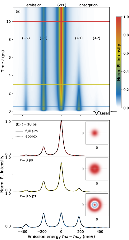
For this reduced model we consider an excitation with a pulse that is detuned by above the ZPL and restrict ourselves to a temperature of K. The simulated PL intensity is shown in Fig. 2(a) color coded as a function of photon emission energy relative to the ZPL and of the time . The most prominent vertical line is the ZPL at energy with additional lines showing phonon emission sidebands () at smaller and absorption sidebands () at higher energies, where marks the number of phonons involved. The laser pulse is spectrally indicated by the black Gaussian at the bottom of the plot and temporally by the arrow on the right.
As explicitly shown in the SM, this detuned excitation drives the phonon subsystem associated with the excited state of the emitter into the state , where is the two-phonon Fock state of the single LO mode. This phonon state is reached with a high fidelity when dephasing and decay, as described by the dissipators in Eq. (2.2), can be neglected during the laser pulse interaction. For the TLS decay time of a few nanoseconds this is definitely fulfilled. But the faster TLS dephasing at room temperature and the phonon decay lead to a less pure phonon state and addmixtures of and are present after the pulse. However, for short times after the pulse in Fig. 2(a) the PSB (+2) is slightly visible, proving that the absorption of two phonons is possible. Due to the decay of the phonons this PSB vanishes within under 2 ps. The same holds for the PSB (+1) which survives significantly longer and is visible until almost 10 ps after the pulse. The reason for the faster decay of the PSB (+2) is, that the transition from the state to the state via the phonon dissipator from Eq. (2cde) is double as fast as the transition from to the displaced vacuum . The probability to lose a phonon is doubled, when there are double as many phonons present.
In contrast to the absorption side, the PSBs on the phonon emission side do not disappear for long times although they initially shrink in amplitude. The reason is that spontaneous and stimulated emission processes contribute to these signals. So as long as phonons are present in the system, stimulated emission makes these processes more likely. When the LO mode is fully decayed into the equilibrium , only spontaneous emission takes place. While all PSBs lose in amplitude, the ZPL increases for two reasons. On the one hand the decay of the excited state happens on a much longer timescale than depicted here and can therefore not be resolved. On the other hand the total PL intensity at a given time, i.e., the spectrally integrated signal of Eq. (2cdg) only depends on the occupation of the TLS, integrated over the spectrometer’s response time . Hence it is constant after the laser pulse on the timescale depicted in Fig. 2. This can be seen by integrating the PL spectrum in Eq. (2cdg) over frequency , forcing . Thus a reduction of the PSBs has to lead to an increase of the ZPL.
To develop a more quantitative picture in Fig. 2(b) we show PL spectra at the specific times marked in (a) by horizontal lines with colors corresponding to the ones in (b). Additionally to each cut an inset depicts the Wigner function of the phonon state associated with the excited state of the TLS, i.e., in the subspace. Focusing first on ps after the pulse (bottom, blue) we see that the phonon absorption sidebands have almost the same height as the emission sidebands. This shows that stimulated processes are more likely than spontaneous ones. The depicted Wigner function has two clear nodes demonstrating that a majority of the phonon occupation is indeed in the state , making the PSB (+2) clearly visible. Moving to a larger time at ps (center, yellow) the PSB (+2) has vanished and the Wigner function shows that already a significant part of the phonon occupation has reached the displaced vacuum state. For a dominating contribution of the state the Wigner function would go to negative values in the middle of the depicted circular distribution. But we find that it only slightly drops, the reason for this being the dominating contribution from the displaced vacuum . For long times at ps (top, red) the phonon absorption sidebands have entirely vanished because the phonons have reached the displaced vacuum state as confirmed by the Gaussian Wigner function. After these 10 ps a quasi-stationary limit is reached whose shape does not change anymore. Only the amplitude of the entire spectrum shrinks further for larger times due to the decay of the excited state of the TLS on a nanosecond timescale. If the signal from Eq. (2cdg) is integrated over time, yielding the typical stationary PL spectrum, it will agree very well with the quasi-stationary limit, since the initial nonequilibrium dynamics of the phonons on a picosecond timescale are negligible compared to the nanosecond timescale of the emitter lifetime.
To understand the PSB dynamics in a slightly more quantitative manner, we take a closer look at the correlation function for times later than the pulse. As explained in detail in the SM, only the phonon part of the density matrix associated with the excited state, i.e., , contributes to the correlation function. We finally obtain an analytical expression that depends on the phonon configuration. For the moment we neglect TLS and LO decay between times and , as they are on a nanosecond and a picosecond timescale, respectively, while the timescale for the delay is given by , which is below 100 fs. We will here only give the expressions for the phonon occupations, i.e., for the case that with being the occupation of the respective displaced Fock state. is the occupation of the TLS, which is taken to be constant after the laser pulse on the picosecond timescale depicted in Fig. 2. Some comments on phonon coherences, i.e., non-diagonal elements of the phonons’ density matrix will be given below. The correlation function associated with the phonon subsystem being in a displaced Fock state at a time after the pulse is given by
| (2cdh) |
as derived in the SM, where the LO decay is neglected between and . We see, that the sum vanishes for and we are left with the result from Ref. [18]. Expanding the exponential function into a series we see that only terms () appear. Therefore no frequencies larger than are possible, meaning that there is no absorption from the phononic vacuum. At , the -term also leads to absorption PSBs. We also see that the correlation function is independent of because the are eigenstates of , and therefore stationary in the absence of decay and laser pulses.
Coherences like lead to a correlation function, that oscillates in with the frequency , as discussed in the SM. Thus, coherences between the eigenstates of in the subspace where is occupied lead to time-dependences of the PL spectrum, in addition to the LO decay. The following two arguments explain why we do not see any such modulations in Fig. 2(a): (A) the phonons are prepared in a state, where there is no coherence, as can be seen in the Wigner functions in Fig. 2(b). Coherences would lead to distributions that depend on the angle [54]. But we only find ones that are symmetric around the center at . These coherences could be created by a laser pulse that has significant spectral overlap with other PSBs or the ZPL, i.e., a laser pulse of duration shorter than fs. The creation of such phonon coherences and phonon quantum beats of optical signals has been achieved in semiconductor quantum wells, coupling to a single LO mode [55, 56, 57]. (B) The smallest frequency of such oscillations in would be with a period of around 23 fs which is significantly shorter than the integration time in Eq. (2cdg). The oscillations would at least be smeared out significantly, reducing their visibility.
To compare with the analytic result from Eq. (3.1) for a given time we insert this result into the correlation function in Eq. (2cdg). We can do so because when is later than the laser pulse and as long as the LO and TLS decay can be neglegted during the delay . At a given time the spectra are added up for each according to the phonon occupation from the numerical simulation. The results are plotted in Fig. 2(b) as dashed black lines. We find an excellent agreement for all considered times. Thus, we conclude that for each time the spectrum can be understood as a superposition of the spectra from each phonon occupation , where we neglect the TLS and LO decay during the integrations over and in Eq. (2cdg). The reason is that the integration time of the filter is relatively short compared to the TLS and LO phonon lifetimes.
3.2 Two LO modes - modelling hBN PL spectra
Our next task is to consider a more realistic model to calculate PL spectra for the hBN emitters. We now assume two dispersionless LO modes, called LO1 and LO2 at energies meV and meV, respectively [18]. The couplings are chosen to be meV, such that . By this choice the ratio between the area under the PSBs and the area under the ZPL is the same as for the single mode case discussed before. We still keep the temperature at K.
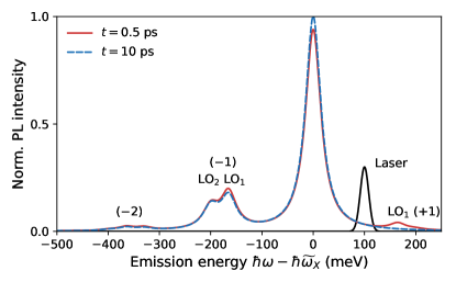
Although the model in the previous section, where only a single LO mode was excited, was introduced as a reduced model, in the following we will demonstrate that by an appropriate optical excitation we can manage to occupy mainly one of the two modes. As depicted in Fig. 3 we use a laser pulse that is detuned by 100 meV above the ZPL and therefore 65 meV below the lower LO1 mode’s PSB (+1). The picture shows two PL spectra, the red solid one is shortly after the laser pulse at ps and the dashed blue one at ps when the excited phonons are entirely decayed. We directly see that both spectra nicely resemble the double peaked PSBs () below the ZPL well known from hBN color centers. Also the characteristic triple peak structure for the () sidebands shows up which is also found in experiment [18]. Focusing on the phonon absorption PSB (+1) above the ZPL we only find a single peak which is the one for the LO1 mode. Obviously mainly this mode gets occupied by the phonon-assisted laser pulse excitation. The LO2 mode at 200 meV is not affected due to its vanishing overlap with the laser and consequently does not show up in the PSB (+1). The fact that mainly LO1 is occupied shortly after the laser pulse can also be seen on the phonon emission side in the PSB (). Here we find that the red curve is slightly larger than the blue dashed one only at the LO1-PSB () energy due to the additional stimulated emission processes of this mode.
The naturally following question is what happens when the laser pulse is tuned exactly between the two first absorption PSBs (+1). The resulting PL spectra directly after the laser pulse at ps are plotted for three different temperatures in Fig. 4(a). The laser pulse spectrum is shown in black, the spectrum at K in red, at 70 K in yellow and at 4 K in blue. All curves represent typical hBN color center spectra with two additional phonon absorption peaks (+1) at 165 meV and 200 meV above the ZPL. Due to the longer dephasing times at lower temperature two features can be identified: (A) All peaks get sharper for lower temperatures and (B) the entire PL signal increases for larger temperatures. While (A) is clear, the reason for (B) lies in the different line widths. The given laser pulse spectrum has a larger overlap with the PSBs (+1) when the lines are broader. This allows for a more efficient off-resonant excitation of the TLS resulting in a stronger PL signal.
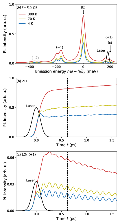
While the resulting spectra are rather obvious, their dynamics provide interesting new aspects. Figures 4(b) and (c) show the temporal evolution of the ZPL and the LO2-PSB (+1), respectively, as marked in (a) by the arrows. The colors correspond to the temperatures in (a). We find that all signals oscillate in time with a period of approximately 0.1 ps. The origin of this is that in the phonon subsystem, associated with the excited state of the TLS, a superposition of the two states and is created. As discussed in the SM, the approximated correlation function in Eq. (3.1) can be extended to multiple modes. As already mentioned in the context of Eq. (3.1), the coherence between the two excited phonon states contributes to the PL signal. For the present case, the quantum beat oscillates with the energy difference between the two states, i.e., with meV which corresponds to a period of 0.12 ps, long enough to be observed despite the finite time resolution of approximately fs.
Comparing the signals for different temperatures, the visibility of the oscillations is better for lower temperatures. The reason is that the dephasing of the TLS during the interaction with the pulse results in a reduction of the purity of the phonon state, as already discussed in the context of the state preparation in the reduced model. The same holds for the coherence resolved here, the faster dephasing at elevated temperatures results in a reduced coherence and consequently in a reduced visibility of the quantum beat. In our model we have not assumed an additional pure dephasing of the phonon modes apart from the dephasing due to their decay. Such an additional dephasing would reduce the visibility on a shorter timescale.
The last aspect to discuss becomes visible when comparing the dynamics of the ZPL in Fig. 4(b) with that of the PSB in (c). Note, that the intensity scale in (c) is much smaller than the one in (b). To compare the dynamics more easily, the vertical dashed lines mark the same time and appear at minima in (b) and at maxima in (c). This shows that the two signals oscillate exactly anti-phased. This effect can be understood when remembering that the full PL signal, integrated over the entire spectrum, only depends on the occupation of the excited state of the TLS, integrated over the spectrometer’s temporal resolution. As the occupation of the excited state decays on a nanosecond timescale, it is virtually constant on the picosecond timescale depicted here. Therefore, when the emission in the PSBs is enhanced, the emission from the ZPL has to be reduced and vice versa. For the same reason all curves in (b) rise after the laser pulse, while the respective sideband in (c) slowly decreases. The dynamics of the remaining PSBs from Fig 4(a) is displayed in the SM for K, showing the in-phase oscillation of all PSBs.
4 Conclusions
In this work we have theoretically investigated the influence of LO phonons on time-dependent PL spectra of a hBN color center. We have first considered a reduced model with only a single LO mode coupling to the color center. In this setting we have studied the influence of phonon decay due to anharmonicities on the PL spectra, focusing mainly on the dynamics of the PSBs. We have found excellent agreement between numerical simulations and a semi-analytical model, which allows us to gain more insight into the role of phonon occupations and phonon coherences on the dynamics of the PL spectra. In a more realistic model we have taken both LO modes with energies of 165 meV and 200 meV into account. This model leads to the characteristic two-peak PSB () known from time-integrated PL spectra of hBN color centers [18]. By using tailored optical excitation schemes we have shown that it is possible to (A) isolate one of the two modes and (B) create coherences between them. In (B) the dynamics of PL spectra exhibit quantum beats due to the 35 meV energy splitting of the two modes. A phonon quantum beat of similar frequency has been measured in semiconductor quantum wells, coupling to a single LO mode with an energy of approximately 35 meV [55]. Our results demonstrate that time-dependent PL spectroscopy is a powerful tool to investigate hBN-SPEs at the same time spectrally and temporally, giving insight into the phonon dynamics of the system.
References
References
- [1] Tran T T, Bray K, Ford M J, Toth M and Aharonovich I 2016 Nat. Nanotechnol. 11 37–41
- [2] Tran T T, Zachreson C, Berhane A M, Bray K, Sandstrom R G, Li L H, Taniguchi T, Watanabe K, Aharonovich I and Toth M 2016 Phys. Rev. Appl. 5 034005
- [3] Tran T T, Elbadawi C, Totonjian D, Lobo C J, Grosso G, Moon H, Englund D R, Ford M J, Aharonovich I and Toth M 2016 ACS Nano 10 7331–7338
- [4] Martínez L J, Pelini T, Waselowski V, Maze J R, Gil B, Cassabois G and Jacques V 2016 Phys. Rev. B 94 121405
- [5] Exarhos A L, Hopper D A, Grote R R, Alkauskas A and Bassett L C 2017 ACS Nano 11 3328–3336
- [6] Tawfik S A, Ali S, Fronzi M, Kianinia M, Tran T T, Stampfl C, Aharonovich I, Toth M and Ford M J 2017 Nanoscale 9 13575–13582
- [7] Sajid A, Reimers J R and Ford M J 2018 Phys. Rev. B 97 064101
- [8] Abdi M, Chou J P, Gali A and Plenio M B 2018 ACS Nano 5 1967–1976
- [9] Gottscholl A, Kianinia M, Soltamov V, Orlinskii S, Mamin G, Bradac C, Kasper C, Krambrock K, Sperlich A, Toth M, Aharonovich I and Dyakonov V 2020 Nat. Mater. 19 540–545
- [10] Sajid A, Ford M J and Reimers J R 2020 Rep. Prog. Phys. 83 044501
- [11] Mendelson N, Chugh D, Reimers J R, Cheng T S, Gottscholl A, Long H, Mellor C J, Zettl A, Dyakonov V, Beton P H, Novikov S V, Jagadish C, Tan H H, Ford M J, Toth M, Bradac C and Aharonovich I 2020 Nat. Mater.
- [12] Konthasinghe K, Chakraborty C, Mathur N, Qiu L, Mukherjee A, Fuchs G D and Vamivakas A N 2019 Optica 6 542–548
- [13] Kianinia M, White S, Fröch J E, Bradac C and Aharonovich I 2020 ACS Photonics 7 2147–2152
- [14] Grosso G, Moon H, Lienhard B, Ali S, Efetov D K, Furchi M M, Jarillo-Herrero P, Ford M J, Aharonovich I and Englund D 2017 Nat. Commun. 8 705
- [15] Mendelson N, Doherty M, Toth M, Aharonovich I and Tran T T 2020 Adv. Mater. 32 1908316
- [16] Axt V M, Machnikowski P and Kuhn T 2005 Phys. Rev. B 71 155305
- [17] Grange T, Somaschi N, Antón C, De Santis L, Coppola G, Giesz V, Lemaître A, Sagnes I, Auffèves A and Senellart P 2017 Phys. Rev. Lett. 118 253602
- [18] Wigger D, Schmidt R, Del Pozo-Zamudio O, Preuß J A, Tonndorf P, Schneider R, Steeger P, Kern J, Khodaei Y, Sperling J, Michaelis de Vasconcellos S, Bratschitsch R and Kuhn T 2019 2D Mater. 6 035006
- [19] Besombes L, Kheng K, Marsal L and Mariette H 2001 Phys. Rev. B 63 155307
- [20] Borri P, Langbein W, Schneider S, Woggon U, Sellin R L, Ouyang D and Bimberg D 2001 Phys. Rev. Lett. 87 157401
- [21] Krummheuer B, Axt V M and Kuhn T 2002 Phys. Rev. B 65 195313
- [22] Förstner J, Weber C, Danckwerts J and Knorr A 2003 Phys. Rev. Lett. 91 127401
- [23] Jakubczyk T, Delmonte V, Fischbach S, Wigger D, Reiter D E, Mermillod Q, Schnauber P, Kaganskiy A, Schulze J H, Strittmatter A, Langbein W, Kuhn T, Reitzenstein S and Kasprzak J 2016 ACS Photonics 3 2461–2466
- [24] Ramsay A J, Gopal A V, Gauger E M, Nazir A, Lovett B W, Fox A M and Skolnick M S 2010 Phys. Rev. Lett. 104 017402
- [25] Zaitsev A M 2000 Phys. Rev. B 61 12909
- [26] Huxter V M, Oliver T A A, Budker D and Fleming G R 2013 Nat. Phys. 9 744–749
- [27] Kehayias P, Doherty M W, English D, Fischer R, Jarmola A, Jensen K, Leefer N, Hemmer P, Manson N B and Budker D 2013 Phys. Rev. B 88 165202
- [28] Jelezko F, Tietz C, Gruber A, Popa I, Nizovtsev A, Kilin S and Wrachtrup J 2001 Single Mol. 2 255–260
- [29] Beha K, Batalov A, Manson N B, Bratschitsch R and Leitenstorfer A 2012 Phys. Rev. Lett. 109 097404
- [30] Glässl M, Barth A M and Axt V M 2013 Phys. Rev. Lett. 110 147401
- [31] Reiter D E, Kuhn T, Glässl M and Axt V M 2014 J. Phys. Condens. Matter 26 423203
- [32] Quilter J H, Brash A J, Liu F, Glässl M, Barth A M, Axt V M, Ramsay A J, Skolnick M S and Fox A M 2015 Phys. Rev. Lett. 114 137401
- [33] Khatri P, Ramsay A J, Malein R N E, Chong H M H and Luxmoore I J 2020 Nano Lett. 20 4256–4263
- [34] Grosso G, Moon H, Ciccarino C J, Flick J, Mendelson N, Mennel L, Toth M, Aharonovich I, Narang P and Englund D 2020 ACS Photonics 7 1410–1417
- [35] Sauer S, Daniels J M, Reiter D E, Kuhn T, Vagov A and Axt V M 2010 Phys. Rev. Lett. 105 157401
- [36] Chu Y, Kharel P, Yoon T, Frunzio L, Rakich P T and Schoelkopf R J 2018 Nature 563 666–670
- [37] Hahn T, Groll D, Kuhn T and Wigger D 2019 Phys. Rev. B. 100 024306
- [38] Kianinia M, Bradac C, Sontheimer B, Wang F, Tran T T, Nguyen M, Kim S, Xu Z, Jin D, Schell A W, Lobo C J, Aharonovich I and Toth M 2018 Nat. Commun. 9 1–8
- [39] Mahan G D 2013 Many-particle physics (Springer Science & Business Media, New York)
- [40] Stauber T, Zimmermann R and Castella H 2000 Phys. Rev. B 62 7336
- [41] Alicki R 2004 Open Syst. Inf. Dyn. 11 53–61
- [42] Roszak K and Machnikowski P 2006 Phys. Lett. A 351 251–256
- [43] Nazir A and McCutcheon D P S 2016 J. Phys. Condens. Matter 28 103002
- [44] Wigger D, Lüker S, Reiter D E, Axt V M, Machnikowski P and Kuhn T 2014 J. Phys. Condens. Matter 26 355802
- [45] Wigger D, Karakhanyan V, Schneider C, Kamp M, Höfling S, Machnikowski P, Kuhn T and Kasprzak J 2020 Opt. Lett. 45 919–922
- [46] Krügel A, Axt V M, Kuhn T, Machnikowski P and Vagov A 2005 Appl. Phys. B 81 897–904
- [47] Breuer H P and Petruccione F 2002 The Theory of Open Quantum Systems (Oxford University Press, Oxford)
- [48] Roy C and Hughes S 2011 Phys. Rev. X 1 021009
- [49] Cuscó R, Artús L, Edgar J H, Liu S, Cassabois G and Gil B 2018 Phys. Rev. B 97 155435
- [50] Mollow B R 1969 Phys. Rev. 188
- [51] Eberly J H and Wodkiewicz K 1977 J. Opt. Soc. Am. 67 1252–1261
- [52] Machnikowski P 2006 Phys. Rev. Lett. 96 140405
- [53] Spokoyny B, Utzat H, Moon H, Grosso G, Englund D and Bawendi M G 2020 J. Phys. Chem. Lett. 11 1330–1335
- [54] Wigger D, Gehring H, Axt V M, Reiter D E and Kuhn T 2016 J. Comput. Electron. 15 1158–1169
- [55] Bányai L, Thoai D B T, Reitsamer E, Haug H, Steinbach D, Wehner M U, Wegener M, Marschner T and Stolz W 1995 Phys. Rev. Lett. 75 2188–2191
- [56] Steinbach D, Kocherscheidt G, Wehner M U, Kalt H, Wegener M, Ohkawa K, Hommel D and Axt V M 1999 Phys. Rev. B 60 12079
- [57] Axt V M, Herbst M and Kuhn T 1999 Superlattice. Microst. 26 117–128