An Experimental Study of Semantic Continuity for Deep Learning Models

Abstract

Deep learning models suffer from the problem of semantic discontinuity: small perturbations in the input space tend to cause semantic-level interference to the model output. We argue that the semantic discontinuity results from these inappropriate training targets and contributes to notorious issues such as adversarial robustness, interpretability, etc. We first conduct data analysis to provide evidence of semantic discontinuity in existing deep learning models, and then design a simple semantic continuity constraint which theoretically enables models to obtain smooth gradients and learn semantic-oriented features. Qualitative and quantitative experiments prove that semantically continuous models successfully reduce the use of non-semantic information, which further contributes to the improvement in adversarial robustness, interpretability, model transfer, and machine bias.

1 Introduction

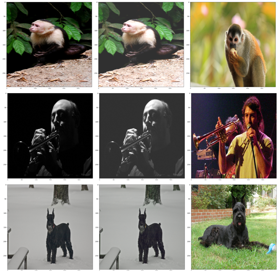
Figure 1: The first column is the original sample $x_{A}$, the second column is the data augmented sample $x_{A^{\prime}}$ by slightly adjusting the brightness, contrast, saturation and hue. And the third column is the picture $x_{B}$ found in the same category. The representation distance between $x_{A}$ and $x_{A^{\prime}}$ is greater than that between $x_{A}$ and $x_{B}$.

The deep learning models can achieve state-of-the-art performance in a wide range of computer vision tasks. However, there are still many weaknesses in deep learning models, one of which is small perturbation can disrupt the models’ outputs. For example, adversarial attacks can cause a devastating diversity of output.

In this paper, we find that many common non-semantic perturbations can also lead to semantic-level interference to the model output, as shown in Fig. 1. The phenomenon shows that the deep learning model is discontinuous in semantic space. The derived samples with the same semantic information should have been in neighborhood  of original samples, and now it is mapped far away from original samples in the models’ output space.

Specifically, semantic continuity means that when the semantic change of the input information is very small, the output of the model will be weakly changed.

In the semantic neighborhood of one sample, there are still a large number of samples that confuse the models or even let the models judge them as wrong categories. The reason is that deep learning models do not make full use of training data.

In deep learning algorithms the utilization of data neighborhood can be divided into two stages. (1) Neighborhood sampling. Data augmentation [1, 2, 18, 27] and adversarial training [14, 7, 3] are the two most typical neighborhood sampling methods. Data augmentation greatly alleviates the overfitting and improves the generalization of deep neural networks. Adversarial training is proposed to solve the problem of adversarial attacks. Adversarial training is a method of injecting adversarial samples into the training set so that the model can fit the original sample and the adversarial sample at the same time. The data augmentation and adversarial training can improve the generalization and robustness of the model to a certain extent, respectively. Many new discoveries prove that adversarial training can bring many additional effects [30, 33, 20, 25, 6, 5, 8, 23, 24, 31, 29], which proves that the reasonable use of the neighborhood samples can make the models perform better. (2) Neighborhood continuity. The neighborhood sampling method generates many semantically similar images, but the outputs of the model to these samples are not similar. We define semantic neighborhood continuity as under the slight perturbation of semantics, the output change of the model is small as well. There is some work that initially utilizes the continuity of the sample neighborhood. For example, with the help of neighborhood continuity, the effect of image similarity search is improved [34]. For example, adversarial logits pairing greatly improves the effect of adversarial training with the help of neighborhood continuity [11].

The goal of this work is to explore in-depth how semantic continuity affects the models. The research on semantic neighborhood continuity is still at a very preliminary stage. The method of neighborhood sampling is just a preliminary use of neighborhood data to improve the generalization of the model. The model trained by the neighborhood sampling method does not learn the relationship between the original data and the data derived from the neighborhood sampling process. The model simply believes that the newly generated data has nothing to do with the original data. The existing neighborhood continuity methods do not explain in-depth why neighborhood continuity has an effect on the model, nor do they find the potential value of neighborhood continuity to the model in multiple fields. Therefore, it is urgent to improve the semantic continuity of deep learning models.

This work discusses the problem of semantic continuity in deep learning models, with the following main contributions:

• We position the semantic discontinuity problem in existing deep learning models and introduce a simple semantic continuity constraint to obtain a smooth gradient and semantic-oriented feature

• We conduct series of experiments and validate the effectiveness of the proposed constraint in increasing semantic continuity and Consequently contribute to improvement in robustness, interpretability, model transfer, and machine bias.

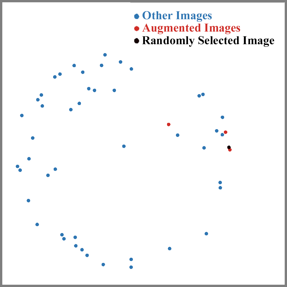
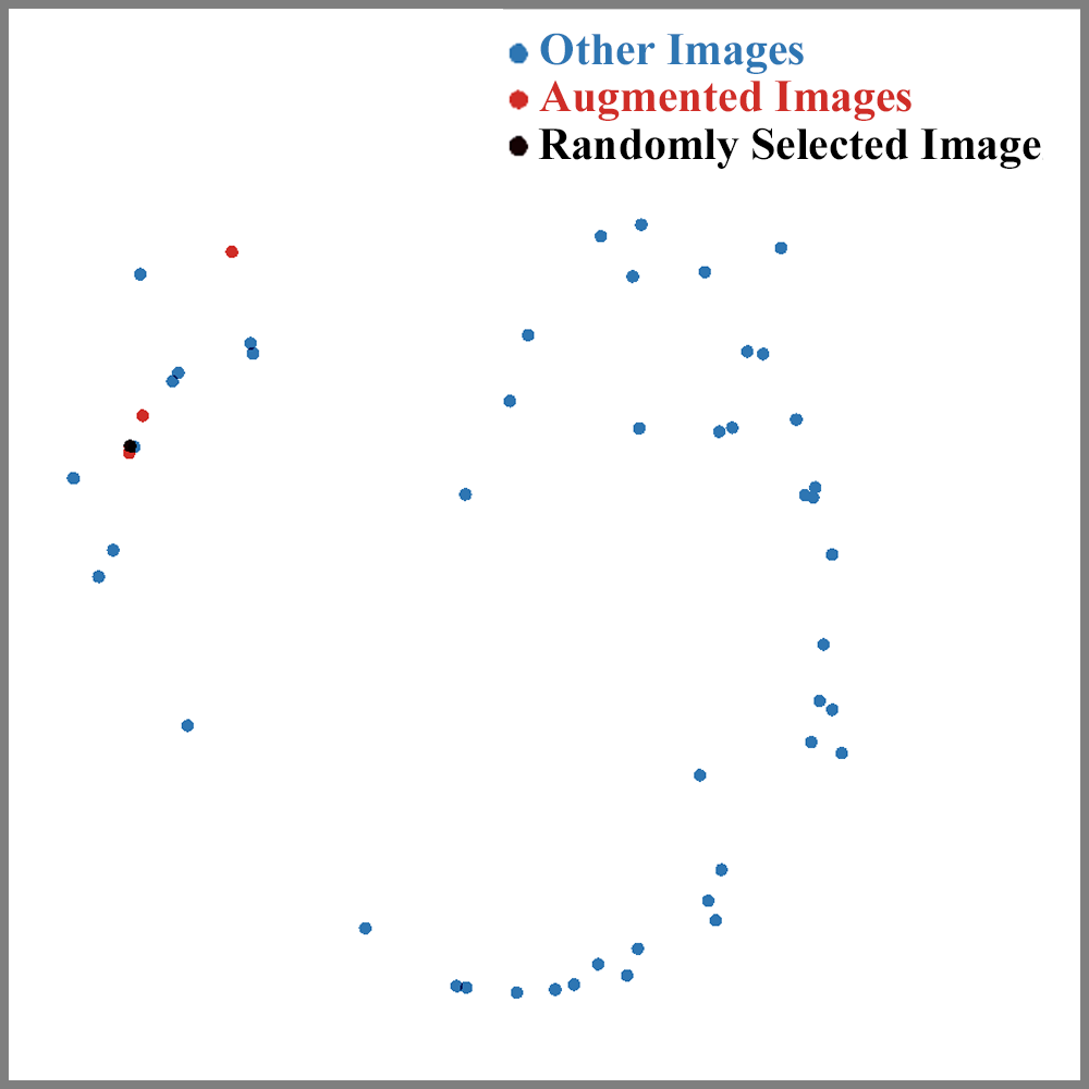
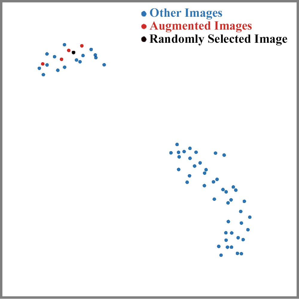
Figure 2: Two-dimensional visualization of the representation of all samples in a certain category of ImageNet Val set. The figure in the left was obtained by PCA, the middle one is the TSNE result, and the right one is the result of UMAP.

2 Semantic Discontinuity is Common

Previous work [3] demonstrated that adversarial samples lead to severe semantic discontinuity problems. This section reports the data analysis results to justify that semantic discontinuity is common which also exists in read-world normal samples under different types of non-semantic perturbations.

2.1 Definition

Before our experiments, we first define some key items to be used in this paper:

1. Image Representation: In this work, the activation value of the Logits layer of the model is specified as the representation of the sample. $F(\cdot)$ is the function to obtain the image representation.

2. Representation Distance: We define Logits Difference(LD) as the distance vector between image representations.

   $$LD(x,x^{\prime})=F(x^{\prime})-F(x)$$ (1)

3. We define Distance Score(DS) as the distance between the two representations.

   $$DS(x,x^{\prime})=||LD(x,x^{\prime})||_{2}^{2}$$ (2)

In this part, we use Resnet50 [9] to conduct experiments in the val set of ImageNet2012 [22, 4].

2.2 Semantic Discontinuity in Normal Samples

Some traditional data augmentation methods can be regarded as non-semantic perturbations, including changing the brightness, contrast, saturation and hue of the image. In our first experiment, we select a picture $x_{A}$ in the Imagenet val set, and randomly choose one of the above four non-semantic perturbations to generate data augmentation sample $x_{A’}$. As shown in Fig 1, it is easy to find samples $x_{B}$ in the same category of $x_{A}$, which satisfies $DS(x_{A},x_{A’})\textgreater DS(x_{A},x_{B})$. This means that the problem of semantic discontinuity is not limited to adversarial samples. During the ordinary training process, the model did not learn the relationship between the sample pairs, only fitted two types of samples.

We further analyze this phenomenon by visualizing the derived representation. We randomly select an image $x_{A}$ in the Imagenet val set, and perform the four data augmentation operations that modify the four attributes of $x_{A}$ respectively. Then we combine the original image $x_{A}$, the four images after data augmentation $\{x_{A^{\prime}_{1}},x_{A^{\prime}_{2}},x_{A^{\prime}_{3}},x_{A^{\prime}_{4}}\}$, and the remaining images of the same category to form a new set $\mathcal{I}_{visualize}$. We send $\mathcal{I}_{visualize}$ to Resnet50 to obtain the image representation. Finally, we visualize the image representation of $\mathcal{I}_{visualize}$ with PCA [32], TSNE [16] and UMAP [17]. It can be seen from Fig. 2 that for all the three visualization methods, the perturbated samples are not the closest samples to the original sample in the representation space. This demonstrates that during the representation learning process, deep models generally lose the correspondence between the original image and its perturbated images. This further justifies the semantic discontinuity existed in the normal image samples.

3 Semantic Continuity Constraints

The semantic discontinuity phenomenon of deep learning models is contrary to human intuition. It is desirable that the deep models understand things in a similar way as humans. To address this goal, we introduce the semantic continuity constraint as the general case for many existing neighborhood continuity methods, and analyze its benefit to the model learning and performance.

We have previously observed that the representation distance(DS) between image pairs becomes unreasonably large under changes that do not affect image semantic information such as data augmentation and adversarial attacks. So we intuitively use DS to constrain the model to improve semantic continuity.

When calculating DS, semantically identical data pairs x and x’ are required, where x refers to the original image and x’ refers to the sample generated by non-semantic perturbation. Here we define in detail how to generate x’:

$$x^{\prime}=P(x),$$ (3)

where $P(\cdot)$ refers to the non-semantic perturbation: data augmentation or adversarial attack.

Based on the above discussion, we design a semantic continuity constraint method based on the Logits layer, and choose data augmentation and adversarial attack as tools to generate non-semantic perturbations.

$$Loss_{continuity}=DS(x,x^{\prime})$$ (4)

Total loss can be defined as:

$$Loss=Loss+\alpha*Loss_{continuity}$$ (5)

where $\alpha$ is the weight of $Loss_{continuity}$.

It is noted that previous neighborhood continuity methods [34, 11] can be seen as special cases of the semantic constraint. Here we give an explanation based on higher-order Taylor decomposition, elaborate on why the semantic continuity constraint can bring gains to the model.

Through the second-order Taylor decomposition, the previously defined LD can be transformed into:

$$LD(x,x^{\prime})=F(x^{\prime})-F(x)=\frac{\partial F}{\partial x}\Delta x+\Delta x^{T}\frac{\partial^{2}F}{\partial x^{2}}\Delta x+R$$ (6)

where R is the remainder of Taylor formula.

At present, data augmentation and adversarial attacks can meet the premise of not changing the semantic information.

In adversarial training, $\Delta x$ can be approximately expressed as:

$$\Delta x=\frac{\partial Loss}{\partial x}\alpha=\alpha\frac{\partial Loss}{\partial F}\frac{\partial F}{\partial x}$$ (7)

Under the semantic continuity constraint, no matter what kind of non-semantic perturbation method is adopted, it will constrain $\frac{\partial F}{\partial x}$ and the higher-order derivative of the term to $x$. The physical meaning of those items represents the impact of a single-pixel on the activation layer. The constraints on those items can limit the models rely on individual pixels, and in turn encourage the models to learn more complex semantic features.

From the Equ. 7 we can see that when adversarial training is used, the constraints on $\frac{\partial F}{\partial x}$ are further enhanced, so the adversarial training will further help the improvement of interpretable phenomena.

It can be seen from the above analysis that semantic continuity leads to smooth input gradients. Smoothing the input gradient will weaken the influence of irrelevant areas and individual pixels, so theoretically semantic continuity can improve the interpretability and robustness of the model, and the robustness will play a role in transfer learning, image generation, feature visualization and other fields [33, 20, 25, 6, 5, 8, 24, 31, 29].

4 Semantic Continuity Improves Deep Learning Models

4.1 Experiment Setting

We carried out experiments on ImageNet2012 and Cifar100 [4, 22, 13], and used Cifar10, SVHN, and MNIST data sets [13, 19, 15] to provide experimental support. We trained four Resnet50 [9] models on ImageNet, common Resnet50, semantic-continuity-constrained Resnet50C, Resnet50ADV for adversarial training and Resnet50ADV+C for semantic continuity adversarial training . On Cifar100, we used Resnet18 to train the above four models. We used the Adam [12] algorithm to optimize; the learning rate was set to 1e-5, $\alpha=1.0$, and PGD [3] was used to generate adversarial samples for adversarial training, and the attack step size was 2pix on Cifar100, $\epsilon=8pix$, 10 iterations; the attack step on ImageNet was 2pix, $\epsilon=16pix$, and it iterated for 10 rounds.

4.2 On Semantic Continuity

For classification tasks, the human decision-making process is insensitive to the image’s brightness, contrast, saturation, and hue transformations. In other words, those changes will not affect the semantic information of the image, but the output of the deep learning model will be affected by these non-semantic perturbations. The semantic continuity loss constraint can effectively improve this deficiency of the deep learning model. We tested the semantic continuity of the four models Resnet18, Resnet18C, Resnet18ADV, and Resnet18ADV+C under the four augmentation methods including brightness, contrast, saturation, and hue. We defined these four augmentation methods with 4 levels as Table 1, and tested the DS of these four models on these 4 level perturbations, as shown in Fig. LABEL:fig:diff_result. It can be clearly seen that the DS of the model with semantic continuity constraints is smaller than that of the original model. In other words, the addition of semantic continuity constraints can diminish the influence on these four non-semantic perturbations, so the semantic continuity of the model has been greatly improved.

Levels	Bright	Contrast	Saturation	Hue
1	16	1.25	1.25	0.1
2	32	1.50	1.50	0.2
3	48	1.75	1.75	0.3
4	64	2.0	2.0	0.4

Table 1: Parameters of different perturbation levels.

In the method designed in this work, the semantic continuity’s weight is represented by the parameter $\alpha$. We measured the accuracy and semantic continuity of Resnet18 with different $\alpha$ in Cifar100. We used the sum of DS under four augmentation methods at level1 to measure the semantic continuity of the models. From Fig. 4, as $\alpha$ increases, the accuracy of the model decreases slightly, but the semantic continuity of the model is significantly improved. For this reason, we finally set $\alpha=1.0$.

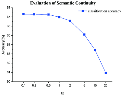
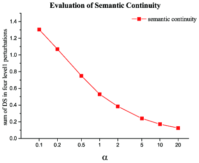
Figure 4: The semantic continuity and classification accuracy under the different setting of $\alpha$. The left figure shows the accuracy of models under different $\alpha$, the right figure shows the semantic continuity of models under different $\alpha$.

4.3 On Semantic Feature

In Sec. 3, we proved that the semantic continuity constraint could make the model’s gradient smoother, and we analyzed that the smooth gradient could make the model less dependent on a single-pixel. Because the single pixel does not have semantic information, we design three experiments to explore whether the semantic-continuity-constrained models use more semantic features.

4.3.1 RGB Channels Translating

As the convolutional neural network has the character of translation invariance, we designed the method of translating RGB three channels to destroy the semantic information of the picture, as shown in Fig. 5. The disturbed image maintains translation invariance on each channel but loses the semantic information.

First, let the R channel translate to the lower right by N pixels, and the G channel to the lower right by N/2 pixels. At the same time, the part that moves out of the edge of the image is added to the upper left of each channel. As the translating distance increases, the picture gradually loses semantic information and becomes a color block that is difficult for people to understand. However, the models can still recognize this type of image.

From Table 6, it can be seen from the comparative experiment that the model with stronger continuity makes less use of this unreasonable translational invariant information, and instead pays more attention on whether there are objects in the image, that is, the model pays more attention to semantic information.

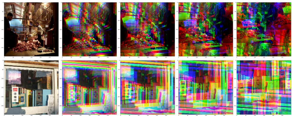
Figure 5: The schematic image of RGB channels translating, the leftmost is the original image, and then the image with N=1/32, 1/16, 1/8, 1/4 side length.

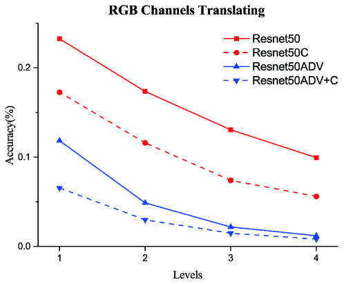
Figure 6: We compared the accuracy of the four models on translated RGB channel images and found that the models with semantic continuity constraints are sensitive to the semantic perturbation.

4.3.2 Randomization Center Area

We observed and counted images in the ImageNet Val set, and found that there are more than 95% pictures in which the task-related information is in the center. So we designed an experiment to disrupt the pixels in the center of the images to eliminate task-related information, as shown in Fig. 7. After disrupting the pixels in the center of the images, most of the task-related information has been destroyed. Although there is a small part of images which have task-related information, we can still see whether the model uses the task-unrelated information. By examining the results in Table 8, it can be determined that the accuracy of the semantic-continuity-constrained model has been more affected, indicating that the semantic-continuity-constrained model pays more attention to the foreground of the images, and uses less task-unrelated information.

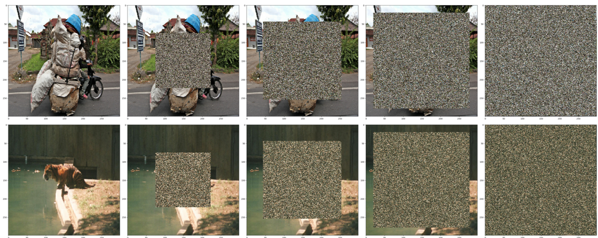
Figure 7: On the left is the original image, followed by schematic images of the image after disrupting 25%,50%,75%,100% of the central part of the images.

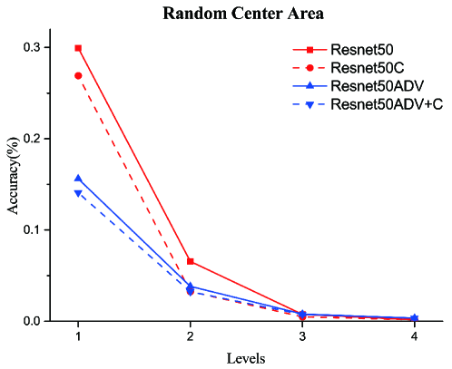
Figure 8: We show the accuracy of the four models for Random Center Area images. The model with higher accuracy uses more task-unrelated information. It can be seen that models with semantic continuity constraint are more dependent on task-related information.

4.3.3 Sliding Puzzle

Inspired by the paper [33], we designed a similar experiment. We divided the image into N image blocks, and disrupted the position of the image blocks as shown in Fig. 9, and then detected the classification accuracy of the re-spliced images by the models. In the case of severe disruption, the image has lost its original semantic information, but the model still has a certain ability to classify the image as shown in Table 10, indicating that the model uses non-semantic information, such as texture information.

It can be seen from the results of the comparative experiment that the model with semantic continuity concentrate decreases its sensitivity to non-semantic information and pays more attention to the semantic information in the image.

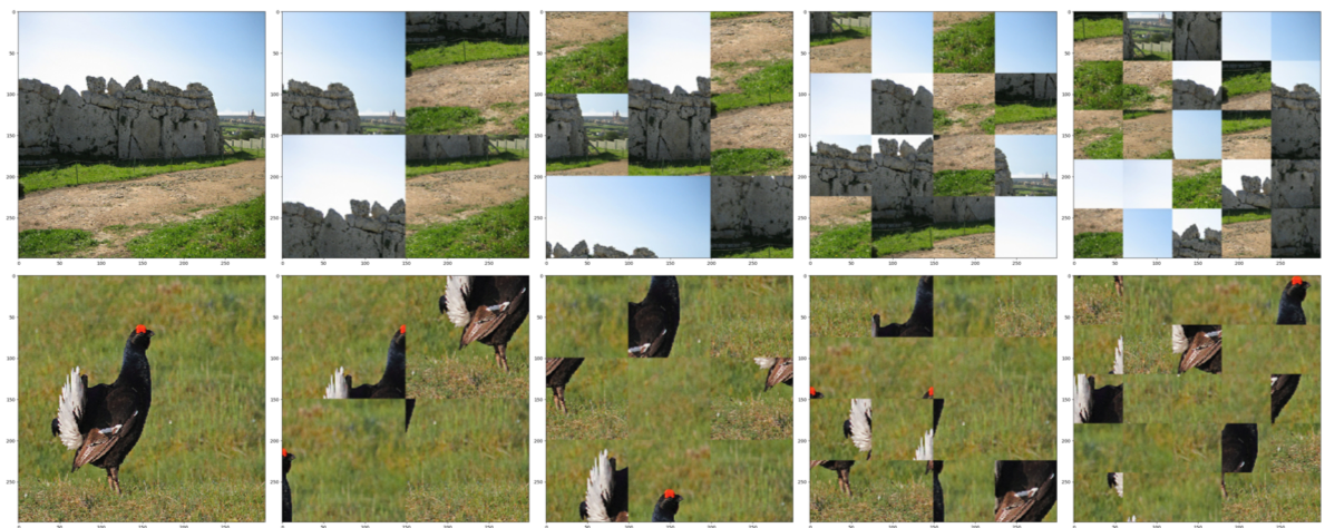
Figure 9: As the number of disturbed image blocks increases, the image gradually loses semantic information. The rapid decline in the classification accuracy of the re-spliced image of the model with the added semantic continuity constraint can explain its reduced dependence on non-semantic information.

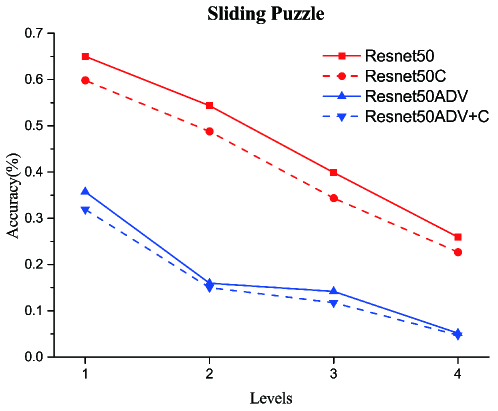
Figure 10: As the number of disturbed image blocks increases, the image gradually loses semantic information. The rapid decline in the classification accuracy of the re-spliced image of the model with continuity constraints can explain its reduced use of non-semantic information.

4.4 On Adversarial Robustness

The analysis in Sec. 3 shows that models with semantic continuity can reduce the impact of a single pixel, and the adversarial attack mainly pixel-level perturbations. Consequently, the model with improved semantic continuity can also improve the adversarial robustness. Thus, we used the PGD algorithm to generate white box adversarial samples to evaluate the model’s adversarial robustness. For the ImageNet2012 and Cifar100 datasets, we set the step size to 2pix, iterating 10 rounds, with an attack setting of $\epsilon=8pix$.

We tested the classification accuracy of adversarial samples on four models derived from the Resnet50 and Resnet18 network structures respectively. Table 2 shows that by adding semantic continuity constraint, the robustness of the adversarially trained model has been greatly improved. Besides, the ordinary training model with semantic continuity will also have a certain defensive effect on adversarial samples. Therefore, the semantic continuity has a huge contribution on models robustness.

	clean accuracy	adv accuracy
Resnet18	66.99%	9.34%
Resnet18C	67.01%	16.01%
Resnet18ADV	63.80%	44.30%
Resnet18ADV+C	59.62%	54.04%

	clean accuracy	adv accuracy
Resnet50	73.42%	0.49%
Resnet50C	72.01%	0.94%
Resnet50ADV	55.43%	8.25%
Resnet50ADV+C	50.66%	32.55%

Table 2: Comparison of the robustness of ordinary training and semantic-continuity-constrained training, clean accuracy represents the classification accuracy on the original images, and adv accuracy represents the classification accuracy on the adversarial samples.

4.5 On Interpretability

In Sec. 4.3, we provide three experiments demonstrating the semantic continuity constraint can increase the models’ usage of semantic features and task-related information. In addition, the semantic continuity constraint can weaken the influence of a single-pixel by smoothing the gradient. Combining the above two points, we speculate that semantic continuity constraint can also bring about an interpretability improvement. In order to verify our conjecture, we choose three interpretable algorithms including Integrated Gradients [28], GradCAM [26] and LIME [21] to observe the improvement of the interpretability of the model by semantic continuity constraint.

4.5.1 Integrated Gradients

Integrated Gradients Method [28] is the improvement of the traditional Saliency Map [10], which is widely used in interpretable tasks nowadays. It uses gradient integration to eliminate the gradient saturation, and the gradient learned by the model can be intuitively seen by this method.

Compared with the traditional Saliency Map, Integrated Gradients Method has a better visualization effect. We tested the performance of the Resnet18 and Resnet50 network structures in the Cifar100 and ImageNet datasets, respectively. Fig. 11 lists some representative interpretable images. Take the third row of ImageNet results as an example. Compared with Resnet50, Resnet50C focuses more on the dog, and at the same time, the gradient perturbations decrease distinctly so that the gradients become smoother. For Resnet50ADV+C, this improvement is more obvious.

As directly recognized from the results, the addition of semantic continuity constraint makes the gradient obtained by the model smoother and more concentrated in the recognized object, thereby greatly improving the interpretability of the model.

Figure 11: The first column is the original image and the second to fifth columns are the gradient saliency maps of the common model, semantic continuity model, robust model, and semantic continuity robust model.

4.5.2 GradCAM

The GradCAM [26] is an algorithm that uses gradient and activation information to visualize the region of interest of the model. We use the GradCAM to observe the model’s attention area to the image under different training constraints. Results respectively show the activation maps of Resnet18 and Resnet50 on the Cifar100 dataset and ImageNet dataset in Fig. 12. Take the first row of data in ImageNet as an example, the Resnet50 model pays more attention to identifying the sky above the snow, while the Resnet50C model focuses more on the snowmobiles and people. This phenomenon is more obvious in Resnet50ADV and Resnet50ADV+C. The area of Resnet50ADV’s attention is looser and more distributed in the background area. In contrast, Resnet50ADV+C’s attention is more focused on the target object. This can prove that the semantic continuity constraint will modify the model’s attention on task-related information and make the model more interpretable.

Figure 12: The first column is the original image and the second to fifth columns are the GradCAM results of the common model, semantic continuity model, robust model, and semantic continuity robust model.

4.5.3 LIME

LIME is a method of analyzing image correlation based on output probability. LIME can evaluate the model output in an objective way. The result is shown in Fig. 13. We take the third row of ImageNet results as an example to analyse the performance of these models. Compared with Resnet50, Resnet50C can be affected by more areas in the bread, indicating that the model is more dependent on the information in the bread. Similarly, it is apparent that Resnet50ADV+C relies on more information in the bread than Resnet50ADV does. This proves that by adding semantic continuity constraint, the result of LIME gets better. The model is more dependent on the information of the task-related information to produce output, while the influence of the task-unrelated information is weakened.

Figure 13: The first column is the original image and the second to fifth columns are the LIME results of the common model, semantic continuity model, robust model, and semantic continuity robust model.

4.6 On Transferability

Robust models always transfer better [24, 31, 29]. The experiments in Sec. 4.4 prove that the semantic continuity constraint can improve the models’ robustness. So we speculate the semantic-continuity-constrained models will have good transferability. Therefore, we tested the transferability of these four models. We use the four Resnet18 models trained by Cifar100 to fine-tunning on the three data sets of Cifar10, SVHN, and MNIST. We find that the model with semantic continuity constraint has a higher accuracy rate, which shows that the model with semantic continuity constraint is helpful to model transferability.

Transfer	Cifar10	SVHN	MNIST
Resnet18	84.61%	94.25%	99.32%
Resnet18C	84.78%	94.60%	99.37%
Resnet18ADV	85.17%	94.66%	99.50%
Resnet18ADV+C	86.40%	94.90%	99.50%

Table 3: The performance of normal training and semantic continuity constraint training in model transfer.

4.7 On Algorithm Fairness

The machine bias has attracted researchers more attention in recent years. The reason for the bias lies in the imbalance of training data. The model will learn the bias and imbalance in data and produce unreasonable outputs, such as gender discrimination. We believe that the key to solving this problem is to let the model minimize the use of task-unrelated information (such as gender) and focus more on task-related information. Previous experiments reveal that semantic continuity constraint can increase the model’s use of semantic information and task-related information. Therefore, we speculate that semantic continuity constraint should also be helpful to the data bias.

We designed a Colorful MNIST dataset to verify our conjecture. The background of 95% data for the training set is red, and that of the left 5% is blue; at the same time, the background of 95% data for testing is blue, and that of the left 5% is red. We use normal training and semantic continuity training methods to fit the training set, and test their performance in the test set. The experimental results are shown in the Table 3.

It shows that the model with semantic continuity constraint uses less task-unrelated information (such as color), and the semantic continuity constraint is helpful to solve the problem of the machine bias.

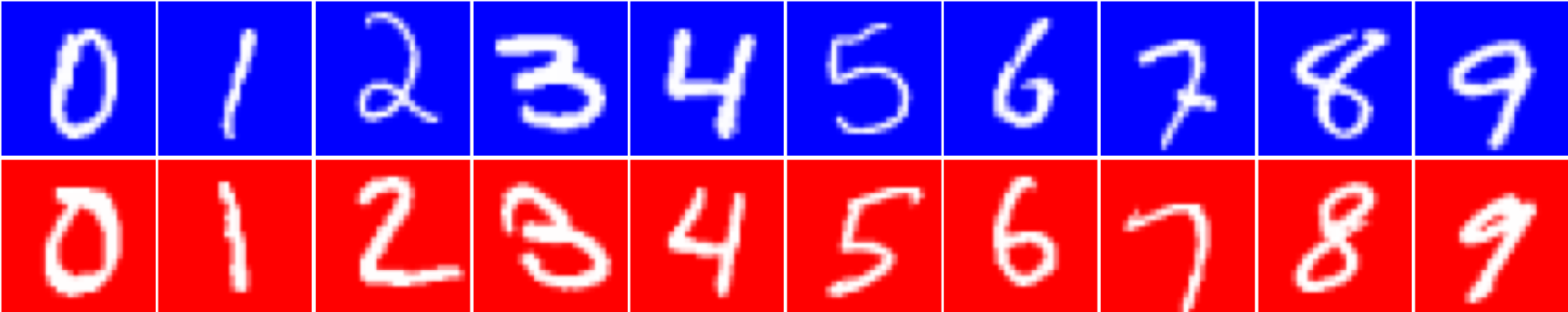
Figure 14: Schematic image of samples in the Color MNIST dataset.

	Color MNIST
Resnet18	96.01%
Resnet18C	97.54%

Table 4: Test performance of ordinary training and semantic continuity constraint training on the Colorful MNIST dataset.

5 Conclusions

This paper systematically analyzes the impact of semantic continuity on deep learning models, and proves the improvement of semantic continuity in terms of robustness, interpretability, model transfer and fairness by experiments. We believe that semantic continuity makes the model’s perception closer to humans’. We will continue to explore the underlying reasons why model semantic continuity improves model performance, and continue to explore the impact of model semantic continuity in the areas of one/few-shot learning, zero-shot learning, and image reconstruction.

References

- [1] Philippe Baecke and Dirk Van den Poel. Data augmentation by predicting spending pleasure using commercially available external data. J. Intell. Inf. Syst., 36(3):367–383, 2011.
- [2] Alexander V. Buslaev, A. Parinov, Eugene Khvedchenya, V. Iglovikov, and A. Kalinin. Albumentations: fast and flexible image augmentations. Inf., 11:125, 2020.
- [3] Nicholas Carlini and David A. Wagner. Towards evaluating the robustness of neural networks. pages 39–57, 2017.
- [4] Jia Deng, W. Dong, R. Socher, L. Li, K. Li, and Li Fei-Fei. Imagenet: A large-scale hierarchical image database. In CVPR 2009, 2009.
- [5] L. Engstrom, Andrew Ilyas, Shibani Santurkar, D. Tsipras, Brandon Tran, and A. Madry. Adversarial robustness as a prior for learned representations. arXiv: Machine Learning, 2019.
- [6] L. Engstrom, Andrew Ilyas, Shibani Santurkar, D. Tsipras, B. Tran, and A. Madry. Learning perceptually-aligned representations via adversarial robustness. ArXiv, abs/1906.00945, 2019.
- [7] Ian Goodfellow, Jonathon Shlens, and Christian Szegedy. Explaining and harnessing adversarial examples. 2015.
- [8] Sachin Goyal, Aditi Raghunathan, Moksh Jain, H. Simhadri, and Prateek Jain. Drocc: Deep robust one-class classification. ArXiv, abs/2002.12718, 2020.
- [9] Kaiming He, X. Zhang, Shaoqing Ren, and Jian Sun. Deep residual learning for image recognition. 2016 IEEE Conference on Computer Vision and Pattern Recognition (CVPR), pages 770–778, 2016.
- [10] T. Kadir and M. Brady. Saliency, scale and image description. International Journal of Computer Vision, 45:83–105, 2004.
- [11] Harini Kannan, A. Kurakin, and Ian J. Goodfellow. Adversarial logit pairing. ArXiv, abs/1803.06373, 2018.
- [12] Diederik P. Kingma and Jimmy Ba. Adam: A method for stochastic optimization. In Yoshua Bengio and Yann LeCun, editors, 3rd International Conference on Learning Representations, ICLR 2015, San Diego, CA, USA, May 7-9, 2015, Conference Track Proceedings, 2015.
- [13] A. Krizhevsky. Learning multiple layers of features from tiny images. 2009.
- [14] Alexey Kurakin, Ian J. Goodfellow, and Samy Bengio. Adversarial examples in the physical world. abs/1607.02533, 2016.
- [15] Y. LeCun, L. Bottou, Yoshua Bengio, and P. Haffner. Gradient-based learning applied to document recognition. 1998.
- [16] L. V. D. Maaten and Geoffrey E. Hinton. Visualizing data using t-sne. Journal of Machine Learning Research, 9:2579–2605, 2008.
- [17] Leland McInnes, John Healy, Nathaniel Saul, and Lukas Großberger. UMAP: uniform manifold approximation and projection. J. Open Source Softw., 3(29):861, 2018.
- [18] Agnieszka Mikołajczyk and M. Grochowski. Data augmentation for improving deep learning in image classification problem. 2018 International Interdisciplinary PhD Workshop (IIPhDW), pages 117–122, 2018.
- [19] Yuval Netzer, T. Wang, A. Coates, A. Bissacco, B. Wu, and A. Ng. Reading digits in natural images with unsupervised feature learning. 2011.
- [20] A. Noack, Isaac Ahern, D. Dou, and Boyang Li. Does interpretability of neural networks imply adversarial robustness? ArXiv, abs/1912.03430, 2019.
- [21] Marco Tulio Ribeiro, Sameer Singh, and Carlos Guestrin. ”why should i trust you?”: Explaining the predictions of any classifier. Proceedings of the 22nd ACM SIGKDD International Conference on Knowledge Discovery and Data Mining, 2016.
- [22] Olga Russakovsky, J. Deng, H. Su, J. Krause, S. Satheesh, S. Ma, Zhiheng Huang, A. Karpathy, A. Khosla, Michael S. Bernstein, A. Berg, and Li Fei-Fei. Imagenet large scale visual recognition challenge. International Journal of Computer Vision, 115:211–252, 2015.
- [23] M. Salehi, Atrin Arya, Barbod Pajoum, Mohammad Otoofi, Amirreza Shaeiri, Mohammad H. Rohban, and H. R. Rabiee. Arae: Adversarially robust training of autoencoders improves novelty detection. ArXiv, abs/2003.05669, 2020.
- [24] Hadi Salman, Andrew Ilyas, L. Engstrom, A. Kapoor, and A. Madry. Do adversarially robust imagenet models transfer better? ArXiv, abs/2007.08489, 2020.
- [25] Shibani Santurkar, D. Tsipras, B. Tran, Andrew Ilyas, L. Engstrom, and A. Madry. Computer vision with a single (robust) classifier. ArXiv, abs/1906.09453, 2019.
- [26] R. R. Selvaraju, Abhishek Das, Ramakrishna Vedantam, Michael Cogswell, D. Parikh, and Dhruv Batra. Grad-cam: Visual explanations from deep networks via gradient-based localization. International Journal of Computer Vision, 128:336–359, 2019.
- [27] Connor Shorten and Taghi M. Khoshgoftaar. A survey on image data augmentation for deep learning. J. Big Data, 6:60, 2019.
- [28] Mukund Sundararajan, Ankur Taly, and Qiqi Yan. Gradients of counterfactuals. CoRR, abs/1611.02639, 2016.
- [29] M. Terzi, A. Achille, M. Maggipinto, and Gian Antonio Susto. Adversarial training reduces information and improves transferability. ArXiv, abs/2007.11259, 2020.
- [30] D. Tsipras, Shibani Santurkar, L. Engstrom, A. Turner, and A. Madry. Robustness may be at odds with accuracy. arXiv: Machine Learning, 2019.
- [31] F. Utrera, Evan Kravitz, N. Erichson, Rekha Khanna, and M. W. Mahoney. Adversarially-trained deep nets transfer better. ArXiv, abs/2007.05869, 2020.
- [32] Svante Wold, Kim Esbensen, and Paul Geladi. Principal component analysis. Chemometrics and intelligent laboratory systems, 2(1-3):37–52, 1987.
- [33] Tianyuan Zhang and Zhanxing Zhu. Interpreting adversarially trained convolutional neural networks. ArXiv, abs/1905.09797, 2019.
- [34] Stephan Zheng, Yang Song, Thomas Leung, and Ian J. Goodfellow. Improving the robustness of deep neural networks via stability training. 2016 IEEE Conference on Computer Vision and Pattern Recognition (CVPR), pages 4480–4488, 2016.