Multipolar exchange interaction and complex order in insulating lanthanides

Abstract

In insulating lanthanides, unquenched orbital momentum and weak crystal-field (CF) splitting of the atomic $J$ multiplet at lanthanide ions result in a highly ranked (multipolar) exchange interaction between them and a complex low-temperature magnetic order not fully uncovered by experiment. Explicitly correlated ab initio methods proved to be highly efficient for an accurate description of CF multiplets and magnetism of individual lanthanide ions in such materials. Here we extend this ab initio methodology and develop a first-principles microscopic theory of multipolar exchange interaction between $J$-multiplets in $f$ metal compounds. The key point of the approach is a complete account of Goodenough’s exchange mechanism along with traditional Anderson’s superexchange and other contributions, the former being dominant in many lanthanide materials. Application of this methodology to the description of the ground-state order in the neodymium nitride with rocksalt structure reveals the multipolar nature of its ferromagnetic order. We found that the primary and secondary order parameters (of $T_{1u}$ and $E_{g}$ symmetry, respectively) contain non-negligible $J$-tensorial contributions up to the ninth order. The calculated spin-wave dispersion and magnetic and thermodynamic properties show that they cannot be simulated quantitatively by confining to the ground CF multiplet on the Nd sites. Our results demonstrate that the ab initio approach to the low-energy Hamiltonian represents a powerful tool for the study of materials with complex magnetic order.

I Introduction

Magnetic insulators with strong spin-orbit coupling on magnetic sites often exhibit unconventional magnetic phases characterized by magnetic multipole moments. Contrary to pure spin systems, the unquenched orbital momentum renders relevant high-ranked components in the magnetic moments of the corresponding magnetic centers, resulting in unconventional magnetic orders and quantum spin liquids. Such multipolar phases can appear in lanthanide and actinide compounds [1, 2, 3, 4, 5, 6, 7, 8, 9, 10, 11, 12, 13, 5, 14, 15, 16, 17, 18, 19], in heavy transition metal systems [20, 21, 22, 23, 24, 25, 26], and possibly in cold atom systems [27].

The multipolar order is often difficult to characterize experimentally because of the lack of response of high-rank multipoles to external perturbations. This situation, for example, has prevented from unraveling the nature of the hidden order phase in URu₂Si₂ for a long time [6]. Another difficulty is the large number of parameters characterizing the intersite multipolar interactions. For example, the total number of independent parameters characterizing the exchange interaction between $J$ multiplets of magnetic centers with open $f$ orbital shells (e.g., lanthanide ions) can be as large as 2079. Besides, the high-rank multipolar structure of magnetic centers gives rise to a complicate tensorial form of electron-lattice coupling which increases the complexity of the low-energy states [28, 8, 1]. From theoretical side, a reliable modeling of multipolar phase also faces problems because only a few interactions are usually considered. For instance, the quadrupole ordering in CeB₆ [7] and the triakontadipole order in NpO₂ [9] have been investigated in this manner. Phenomenological approaches always encounter the following issues: (1) it is not possible to know a priori the dominant contribution among the multipolar interactions and (2) it is unclear what is the actual impact of the remaining part of the interactions.

The multipolar order could be, in principle, quantitatively analyzed by combining the microscopic theory and quantum chemistry approaches. Attempts to build such connection have been undertaken in the past for various compounds [29, 30, 31, 32, 33, 34, 8, 35]. Recently, a microscopic theory of the superexchange interaction between the ground atomic $J$ multiplets has been developed for the $f$ metal compounds [1, 36]. The developed microscopic model in combination with first principles calculations enables to accurately determine all multipolar interactions from several tens of input microscopic parameters. By this approach, the multipolar interactions in a family of lanthanide-radical single-molecule magnets were determined and on this basis the relaxation path of magnetization was established [37, 38]. It appears very tempting to extend this approach to the ab initio study of multipolar order in lanthanide based magnetic insulators.

In lanthanides, the multiconfigurational structure of low-lying multiplets arises from a subtle competition between electrostatic and covalent effects in the crystal field (CF) of surrounding ligands [39]. While such level of treatment of the electronic structure cannot be attained by single-determinant methods like Hartee-Fock approximation (HF) or density functional theory (DFT), explicitly correlated ab initio post Hartree-Fock (HF) methods based on complete active space self-consistent field (CASSCF) [40, 41] were recently found highly efficient for accurate description of CF multiplets and magnetism of lanthanide (Ln) centres in various materials [39, 42, 43]. This approach cannot be directly applied at the same level of accuracy to complexes and fragments with more than one Ln ion, which has hampered a straightforward derivation of low-energy Hamiltonian describing their multipolar exchange interaction. However, given a very strong localization of multiplets’ wave functions at Ln centers, second-order electron transfer processes involving Ln $4f$ orbitals are sufficient for an adequate description of kinetic contribution to exchange interaction [1, 36]. Such electron transfer processes between Ln $4f$ orbitals have been recently considered for the investigation of exchange interaction in Ln-radical pairs [37, 38]. However, for a quantitative description of Ln-Ln exchange interaction, besides virtual electron transfer between magnetic $4f$ orbitals, it is indispensable also to take into account the electrons delocalization from them to $5d$ and other empty Ln orbitals at neighbor magnetic centers, which gives rise to the Goodenough’s exchange contribution.

We would like to stress the major difference between the exchange interaction in transition metal and lanthanide magnetic insulators. In the former, the usual situation is that the antiferromagnetic Anderson’s superexchange is absolutely dominant when not forbidden by symmetry rules, exceeding by ca an order of magnitude all other exchange contributions and leading, therefore, to strong antiferromagnetism. A known example in this paradigm is, e.g., the strong antiferromagnetism in La₂CuO₄ [44]. Exceptions arise when the overlap of magnetic orbitals is weak or exactly zero on symmetry grounds (Goodenough-Kanamori-Anderson rules [45, 46, 47]) and when Anderson’s description of exchange interaction is not appropriate [48]. Then materials may become ferromagnetic due to dominating potential exchange and/or ligands’ spin polarization mechanism in the former case and kinetic ferromagnetic superexchange in the latter case. On the contrary, in lanthanides the Goodenough’s exchange mechanism is often dominant because of a much stronger hybridization of magnetic $4f$ orbitals with empty orbitals of excited Ln shells due to a strong admixture of bridging ligands’ orbitals. When the geometry of the bridge and the symmetry of magnetic $4f$ orbitals favor strong orbital interaction with empty Ln orbitals, a relatively strong ferromagnetism arises due to this Goodenough’s mechanism as, e.g. in the series of Dy_nSc_3-nN@C₈₀, $n$ = 1,2,3, complexes [49, 50]. Note that this scenario is valid for Ln-Ln pairs and not for Ln-radical ones which can exhibit a very strong antiferromagnetism [51, 52, 37, 53, 54]. Along with exchange interaction, a dipolar magnetic interaction should be considered too when treating the pairs of lanthanide ions. None of the mentioned interactions can be neglected a priori in this case and should, therefore, be accounted for as contributions to the overall multipolar magnetic coupling. Such a comprehensive treatment of exchange contributions and multipolar magnetic interaction has never been attempted by ab initio methods so far.

Here we extend the ab initio approach proved successful for the description of mononuclear lanthanide complexes and fragments to the treatment of exchange interaction and develop on its basis a first-principles microscopic theory of multipolar magnetic coupling between $J$-multiplets in $f$ metal compounds. The key point of the approach is a complete account of Goodenough’s exchange mechanism along with traditional Anderson’s superexchange and other contributions.

The developed theory is applied to the investigation of the multipolar order in prototypical lanthanide magnetic insulator, neodymium nitride NdN, a member of a vast family of lanthanide nitrides exhibiting ferromagnetism with high critical (Curie) temperature of about a few tens K [55]. The ferromagnetic transition does not change the x-ray diffraction patterns, indicating the irrelevance of electron-lattice interaction [56]. Besides, the magnetism in the entire family does not depend much on the kind of rare-erath ions, suggesting the primary role of intersite magnetic interaction rather than single-ion properties and prompting simple models for the explanation of its ferromagnetism [57]. Despite this apparent simplicity, our analysis unravel a complex magnetic order in NdN described by primary and secondary order parameters and containing non-negligible $J$-tensorial contributions up to the ninth order. At the same time the first-principles theory reproduces well the known experimental data on the observed ferromagnetic phase. Finally, the fingerprints of multipolar order in the low-energy excitations and magnetic and thermodynamic properties are analyzed and explored.

II Multipolar superexchange interaction

Because of a strong localization of magnetic $4f$ orbitals, the multipolar exchange interaction Hamiltonian for lanthanide magnetic insulators can be derived from a microscopic Hamiltonian within Anderson’s superexchange theory [45, 58]. In Sec. II.1, the microscopic Hamiltonian is introduced. In Sec. II.2, the local crystal-field model is derived. Due to a strong localization of $4f$ orbitals and their weak hybridization with ligands’ orbitals, the low-energy electronic states at Ln sites are well described by weakly crystal-field (CF) split atomic $J$ multiplets [59]. The corresponding CF operators are conveniently represented by irreducible tensor operators defined on the corresponding $J$ multiplets, hereafter referred to as crystal-field model. In Sec. II.3, the intersite interaction model acting on the ground $J$ multiplets on Ln sites is derived. Previous microscopic theory [36] is extended here to include the Goodenough’s contribution [60, 47] due to virtual electron transfers between the partially filled $f$ and empty $d$ and other orbitals. The derived exchange interaction is transformed into the irreducible tensor form, i.e., the multipolar exchange interaction Hamiltonian.

II.1 Microscopic Hamiltonian

The microscopic Hamiltonian $\hat{H}$ for an insulating $f$ metal compound contains all the essential interactions. The Hamiltonian is written as

$$\hat{H} = \sum_{i}\hat{H}^{i}_{\text{loc}}+\hat{H}_{\text{C}}+\hat{H}_{\text{PE}}+\hat{H}_{\text{t}}.$$ (1)

The first term $\hat{H}_{\text{loc}}^{i}$ contains the single $f$ ion Hamiltonians at site $i$,

$$\hat{H}^{i}_{\text{loc}} = \hat{H}^{i}_{\text{orb}}+\hat{H}^{i}_{\text{C}}+\hat{H}^{i}_{\text{SO}}.$$ (2)

These terms include the orbital splittings, on-site Coulomb, and spin-orbit couplings, respectively. The other terms are intersite Coulomb ($\hat{H}_{\text{C}}$), potential exchange ($\hat{H}_{\text{PE}}$), and electron transfer ($\hat{H}_{\text{t}}$) interactions. The present model includes only the orbitals on magnetic centers in the spirit of Anderson’s theory [45]. The relevant orbitals are partially filled $f$ $(l_{f}=3)$ and empty $d$ $(l_{d}=2)$ and $s$ $(l_{s}=0)$ orbitals.

The explicit form of the local Hamiltonian $\hat{H}_{\text{loc}}$ (2) is the following. The first term ($\hat{H}_{\text{orb}}^{i}$) includes the atomic orbital energies and the CF splitting,

$$\hat{H}_{\text{orb}}^{i} = \sum_{lmm^{\prime}}\left(H^{i}_{l}\right)_{mm^{\prime}}\hat{a}_{ilm\sigma}^{\dagger}\hat{a}_{ilm^{\prime}\sigma}.$$ (3)

Here $l$ and $m$ are the quantum numbers for the atomic orbital angular momentum $\hat{\bm{l}}^{2}$ and its $z$ component $\hat{l}_{z}$, respectively, $\hat{a}_{ilm\sigma}^{\dagger}$ ($\hat{a}_{ilm\sigma}$) are the electron creation (annihilation) operators in the orbital $lm$ with the component of electron spin $\sigma$ ($=\pm 1/2$) on site $i$ , and $(H_{l})_{mm^{\prime}}$ are the matrix elements of the one-electron Hamiltonian. The second term ($\hat{H}_{\text{C}}^{i}$) in Eq. (2) consists of the atomic electrostatic interaction between the electrons in the $f$ shell and those between the $f$ and the $d$ or $s$ orbitals (see for concrete expressions Sec. II in Ref. [62]). The last term ($\hat{H}_{\text{SO}}^{i}$) of Eq. (2) is the spin-orbit coupling,

$$\hat{H}_{\text{SO}}^{i} = \sum_{lm\sigma m^{\prime}\sigma^{\prime}}\lambda_{l}\langle lms\sigma|\hat{\bm{l}}\cdot\hat{\bm{s}}|lm^{\prime}s\sigma^{\prime}\rangle\hat{a}^{\dagger}_{ilm\sigma}\hat{a}_{ilm^{\prime}\sigma^{\prime}},$$ (4)

where $\lambda_{l}$ is the spin-orbit coupling parameter for the $l$ orbital, $s=1/2$ is electron spin, $\hat{\bm{s}}$ the electron spin operator, and $|lms\sigma\rangle$ are the spin-orbital decoupled states. Among the local interactions (2), only $\hat{H}_{\text{orb}}^{i}$ may break the spherical symmetry of the model.

The explicit form of the intersite interactions in Eq. (1) is the following. The intersite $\hat{H}_{\text{C}}$ and $\hat{H}_{\text{PE}}$ are, respectively,

$$\hat{H}_{\text{C/PE}}= \frac{1}{2}\sideset{}{{}^{\prime}}{\sum}_{ij(i\neq j)}\hat{H}_{\text{C/PE}}^{ij},$$ (5)

$$\hat{H}_{\text{C}}^{ij}= \sum_{lm\sigma}(ilm,jl^{\prime}m^{\prime}|\hat{g}|iln,jl^{\prime}n^{\prime})$$

$$\times\hat{a}_{ilm\sigma}^{\dagger}\hat{a}_{iln\sigma}\hat{a}_{jl^{\prime}m^{\prime}\sigma^{\prime}}^{\dagger}\hat{a}_{jl^{\prime}n^{\prime}\sigma^{\prime}},$$ (6)

$$\hat{H}_{\text{PE}}^{ij}= \sum_{lm\sigma}-(ilm,jl^{\prime}m^{\prime}|\hat{g}|jl^{\prime}n^{\prime},iln)$$

$$\times\hat{a}_{ilm\sigma}^{\dagger}\hat{a}_{iln\sigma^{\prime}}\hat{a}_{jl^{\prime}m^{\prime}\sigma^{\prime}}^{\dagger}\hat{a}_{jl^{\prime}n^{\prime}\sigma}.$$ (7)

Here $\sum_{lm\sigma}$ is the sum over all orbital and spin angular momenta, $\hat{g}$ is the Coulomb interaction operator between electrons, and $(ilm,jl^{\prime}m^{\prime}|\hat{g}|iln,jl^{\prime}n^{\prime})$ and $(ilm,jl^{\prime}m^{\prime}|\hat{g}|jl^{\prime}n^{\prime},iln)$ are the matrix elements. The electron transfer interaction is expressed by

$$\hat{H}_{\text{t}} = \sideset{}{{}^{\prime}}{\sum}_{ij(i\neq j)}\sum_{lml^{\prime}m^{\prime}\sigma}t^{ij}_{lm,l^{\prime}m^{\prime}}\hat{a}_{ilm\sigma}^{\dagger}\hat{a}_{jl^{\prime}m^{\prime}\sigma},$$ (8)

where $t^{ij}_{lm,l^{\prime}m^{\prime}}$ indicate the electron transfer parameters between sites $i$ and $j$.

The knowledge on the energy scales of the microscopic interactions is decisive to construct the low-energy states in Sec. II.2.2 and II.3. In the case of the lanthanide systems, the on-site Coulomb interaction is the strongest (5-7 eV) [63], which is followed by the on-site spin-orbit coupling ($\lambda_{f}\approx$ 0.1 eV) [59], and the $4f$ orbital splitting due to the hybridization with the environment (3) [64, 39] and the electron transfer interaction parameters (8) between $f$-shells (about 0.1-0.3 eV). The intersite Coulomb interaction (6) is expected to be a few times weaker than the on-site Coulomb interaction and the intersite potential exchange interaction (7) will be a few orders of magnitude smaller than the Coulomb interaction. The local interactions and the intersite Coulomb interaction are much stronger than the remaining intersite interactions. The situation is similar to those of actinide compounds. Therefore, the same approach applies to actinides [1], though the stronger delocalization of the $5f$ orbitals than the $4f$ orbitals weakens the intrasite interactions, while enhances the CF and intersite interactions [59].

II.2 Crystal field model

In this section, the low-energy eigenstates of single $f^{N}$ ion are derived, and on this basis the CF model is constructed. Among the microscopic interactions in the model (1), the eigenstates of a $f^{N}$ ion are in the first place determined by the intra-atomic Coulomb interaction and then by the spin-orbit coupling. Thus derived atomic states are weakly CF split. As mentioned above, the CF splitting of the atomic $J$ multiplet is described through irreducible tensor operators acting in the space of this multiplet.

Throughout Sec. II.2, the index for site $i$ is omitted for simplicity.

II.2.1 Crystal-field states

The degeneracy of $f^{N}$ configurations is lifted by the intra-atomic exchange (Hund) coupling in $\hat{H}_{\text{C}}$. The eigenstates of $\hat{H}_{\text{C}}$, the $LS$-terms, are characterized by the total orbital $\hat{\bm{L}}$ and spin $\hat{\bm{S}}$ angular momenta because of the spherical symmetry of $\hat{H}_{\text{C}}$:

$$\hat{H}_{\text{C}}|f^{N}\alpha LM_{L}SM_{S}\rangle=E_{\text{C}}(f^{N}\alpha LS)|f^{N}\alpha LM_{L}SM_{S}\rangle,$$

(9)

Here $L$ ($S$) is the quantum number for the orbital (spin) angular momentum, $M_{L}$ ($M_{S}$) is the eigenvalue of $\hat{L}_{z}$ ($\hat{S}_{z}$), $\alpha$ distinguishes the repeated $LS$-terms and $E_{\text{C}}(f^{N}\alpha LS)$ is the eigenenergy. $LS$-terms are $[L][S]$-fold degenerate, where $[x]=2x+1$.

The $LS$-terms are split into $J$-multiplets by the spin-orbit coupling $\hat{H}_{\text{SO}}$:

$$\left(\hat{H}_{\text{C}}+\hat{H}_{\text{SO}}\right)|f^{N}\alpha JM_{J}\rangle=E_{J}(f^{N}\alpha J)|f^{N}\alpha JM_{J}\rangle.$$

(10)

Here $J$ and $M_{J}$ are, respectively, the quantum numbers for the total angular momentum operators, $\hat{\bm{J}}=\hat{\bm{L}}+\hat{\bm{S}}$ and $\hat{J}_{z}$, respectively, and $\alpha$ distinguishes the repeated $J$-multiplets, .

The ground $J$-multiplet states $|f^{N}\alpha JM_{J}\rangle$ are approximated by linear combinations of the lowest $LS$-terms when the hybridization between the ground and the excited $LS$-terms by $\hat{H}_{\text{SO}}$ can be ignored:

$$|f^{N}JM_{J}\rangle = \sum_{M_{L}M_{S}}|f^{N}LM_{L}SM_{S}\rangle(JM_{J}|LM_{L}SM_{S}).$$

(11)

Here $(JM|LM_{L}SM_{S})$ are the Clebsch-Gordan coefficients [66, 67] . $\alpha$ is not written in Eq. (11) because each $J$ appears only once. This approximation is often adequate for the description of the ground states of the lanthanide and actinide ions. Eq. (11) becomes the basis for the description of the low-energy states of embedded $f$ ion (hereafter $L$, $S$, and $J$ stand for the angular momenta for the ground $LS$-term and the ground $J$ multiplet of the $f$ metal ion, respectively).

The ground $J$ multiplets are slightly split by the weak hybridization between the $f$ orbitals and the surrounding ligands. The local quantum states are obtained by solving the equation:

$$\left(\hat{H}_{\text{loc}}+\hat{H}_{\text{int}}\right)|f^{N}\nu\rangle = E(f^{N}\nu)|f^{N}\nu\rangle.$$ (12)

$\hat{H}_{\text{int}}$ stands for a potential which originates from some parts of Coulomb and potential exchange interactions from the environment of the Ln ion. The splitting of the $J$ multiplet occurs due to the low-symmetric components in $\hat{H}_{\text{orb}}$ and $\hat{H}_{\text{int}}$. The low-energy CF states $|f^{N}\nu\rangle$ can be expressed by the linear combinations of the ground atomic $J$ multiplet states,

$$|f^{N}\nu\rangle = \sum_{M_{J}}|f^{N}JM_{J}\rangle C_{JM_{J},\nu},$$ (13)

with the expansion coefficients $C_{JM_{J},\nu}$ ($\nu=0,1,...,2J$), which define a $[J]$-dimensional unitary transformation matrix from $|f^{N}JM_{J}\rangle$ to $|f^{N}\nu\rangle$ states. This transformation assumes negligible mixing of the ground and excited $J$-multiplets ($J$-mixing), which is often fulfilled in lanthanide and actinide systems because the energy gaps between the ground and the excited $J$ multiplets ($\gtrsim\lambda_{f}J$) are much larger than the CF splitting. The weakly CF split $J$ mutiplet (13) is employed in the derivation of analytical form of the exchange interaction below, whereas the not-explicitly-included effects of the $J$-mixing are recovered at the level of derivation of model parameters from ab initio calculations of Ln fragments.

II.2.2 Model CF Hamiltonian

The CF Hamiltonian is derived by transforming the low-energy part of the local Hamiltonian into irreducible tensor form within the ground $J$ multiplets [59]. The transformation consists of two steps: projection of the local Hamiltonian ($\hat{H}_{\text{loc}}+\hat{H}_{\text{int}}$) into the space of the ground atomic $J$ multiplets,

$$\mathcal{H}_{J}=\{|f^{N}JM_{J}\rangle|M_{J}=-J,-J+1,...,J\},$$ (14)

and the expansion of the Hamiltonian with the irreducible tensor operators. First, the local Hamiltonian in Eq. (12) is projected into the Hilbert space $\mathcal{H}_{J}$:

$$\hat{H}_{\text{CF}}=\hat{P}_{J}\left(\hat{H}_{\text{loc}}+\hat{H}_{\text{int}}\right)\hat{P}_{J},$$ (15)

where $\hat{P}_{J}$ is the projection operator into $\mathcal{H}_{J}$ (14),

$$\hat{P}_{J}=\sum_{M_{J}}|f^{N}JM_{J}\rangle\langle f^{N}JM_{J}|.$$ (16)

This procedure entails the approximation employed in Eq. (13). Then introducing the irreducible tensor operators [1, 69, 67] (see also Sec. I E in SM [62]) ,

$$\hat{T}_{kq}= \sum_{M_{J}N_{J}}(-1)^{J-N_{J}}(kq|JM_{J}J-N_{J})$$

$$\times|f^{N}JM_{J}\rangle\langle f^{N}JN_{J}|,$$ (17)

Eq. (15) is rewritten as

$$\hat{H}_{\text{CF}} = \sum_{kq}\mathcal{B}_{kq}\hat{T}_{kq}.$$ (18)

From the triangle inequality for the Clebsch-Gordan coefficients in Eq. (17), ranks $k$ are integers satisfying

$$0\leq k\leq 2J.$$ (19)

The CF parameters $\mathcal{B}_{kq}$ are calculated as

$$\mathcal{B}_{kq} = \text{Tr}\left[\hat{T}_{kq}^{\dagger}\hat{H}_{\text{CF}}\right]$$ (20)

with $\hat{H}_{\text{CF}}$ from Eq. (15). The trace (Tr) is on $\mathcal{H}_{J}$ (14).

The symmetry properties of $\hat{H}_{\text{CF}}$ are imprinted in $\mathcal{B}_{kq}$. The Hermiticity of $\hat{H}_{\text{CF}}$, $\hat{H}_{\text{CF}}^{\dagger}=\hat{H}_{\text{CF}}$, leads to

$$\mathcal{B}_{kq}^{*} = (-1)^{q}\mathcal{B}_{k-q}.$$ (21)

The time-eveness, $\Theta\hat{H}_{\text{CF}}\Theta^{-1}=\hat{H}_{\text{CF}}$ [59], makes $\mathcal{B}_{kq}\neq 0$ if and only if

$$k\in\text{even positive integers}$$ (22)

under the constraint (19). If the CF Hamiltonian is given by the $f$ shell model, the upper bound of $k$ becomes $\min(2J,2l_{f}+1)$. When $2J>2l_{f}+1$ as occurs in many $f$ elements, the number of CF parameters is at most 27, i.e., much less than the number of the matrix elements of general $2J$-dimensional Hermitian matrices. The number is further reduced when the system has spatial symmetry.

The CF Hamiltonian is sometimes expressed by the tesseral tensors introduced below instead of $\hat{T}_{kq}$. $\hat{T}_{kq}$ (17) may be transformed into “real” and “imaginary” (tesseral) tensors [see Eq. (10) in Ref. [1]]. For $q=0$,

$$\hat{O}^{0}_{k} = \hat{T}_{k0},$$ (23)

and for $q>0$,

$$\hat{O}^{-q}_{k} = \frac{i}{\sqrt{2}}\left[-(-1)^{q}\hat{T}_{k-q}+\hat{T}_{kq}\right],$$

$$\hat{O}^{q}_{k} = \frac{1}{\sqrt{2}}\left[\hat{T}_{k-q}+(-1)^{q}\hat{T}_{kq}\right].$$ (24)

In the follwing sections, the tesseral tensor form is sometimes used.

II.3 Effective intersite interaction

Starting from the microscopic Hamiltonian (1), first, the effective low-energy model is derived in Sec. II.3.1. Subsequently, the low-energy model is cast into the irreducible tensor (multipolar) form (Sec. II.3.2).

II.3.1 General form

The microscopic Hamiltonian (1) is transformed into an effective model on a low-energy Hilbert space,

$$\mathcal{H}_{0}=\bigotimes_{i}\mathcal{H}_{J}^{i},$$ (25)

using the Anderson’s superexchange approach [45, 58], which is appropriate for insulating lanthanides as mentioned above. Here $\mathcal{H}_{J}^{i}=\{|f^{N_{i}}J_{i}M_{J}\rangle\}$, Eq. (14). The microscopic Hamiltonian (1) is divided into the unperturbed $\hat{H}_{0}$ and perturbation $\hat{V}$ parts:

$$\hat{H}_{0} = \sum_{i}\left(\hat{H}_{d}^{i}+\hat{H}_{s}^{i}+\hat{H}_{\text{C}}^{i}+\hat{H}_{\text{SO}}^{i}\right)+\hat{H}_{\text{C}}^{(0)},$$ (26)

$$\hat{V} = \sum_{i}\hat{H}_{f}^{i}+\left(\hat{H}_{\text{C}}-\hat{H}_{\text{C}}^{(0)}\right)+\hat{H}_{\text{PE}}+\hat{H}_{\text{t}}.$$ (27)

Here the orbital term $\hat{H}_{\text{orb}}$ (3) is divided into the $f$, $d$, and $s$ terms ($\hat{H}_{f}$, $\hat{H}_{d}$, and $\hat{H}_{s}$, respectively), and $\hat{H}_{\text{C}}^{(0)}$ is the classical intersite Coulomb interaction $u^{\prime}\hat{n}_{i}\hat{n}_{j}$, where $u^{\prime}$ is the intersite Coulomb repulsion parameter and $\hat{n}_{i}=\sum_{m\sigma}\hat{a}_{ifm\sigma}^{\dagger}\hat{a}_{ifm\sigma}$. $\hat{H}_{0}$ in (26) is defined in a form that ensures the degeneracy of its eigenvalues within $\mathcal{H}_{0}$:

$$\hat{H}_{0}\hat{P}_{0}=E_{0}\hat{P}_{0},$$ (28)

where $\hat{P}_{0}=\bigotimes_{i}\hat{P}_{J}^{i}$ and $\hat{P}_{J}^{i}$ is given by Eq. (16). Applying the second order perturbation theory, the effective Hamiltonian $\hat{H}_{\text{eff}}$ is derived (see, e.g., Ch. XVI in Ref. [71]):

$$\hat{H}_{\text{eff}} =E_{0}\hat{P}_{0}+\hat{P}_{0}\hat{V}\hat{P}_{0}+\hat{P}_{0}\hat{V}\frac{\hat{Q}_{0}}{a}\hat{V}\hat{P}_{0}.$$ (29)

$$\frac{\hat{Q}_{0}}{a} =\sum_{\kappa\notin\mathcal{H}_{0}}\hat{P}_{\kappa}\frac{1}{E_{0}-\hat{H}_{0}}\hat{P}_{\kappa}.$$ (30)

Here $\kappa$ denotes quantum states not included in $\mathcal{H}_{0}$, i.e., excited (non-magnetic) $f^{N}$ states on Ln sites and one-electron transferred states. Substituting $\hat{H}_{0}$ (26) and $\hat{V}$ (27) into $\hat{H}_{\text{eff}}$ (29), the following form of the effective Hamiltonian is derived:

$$\hat{H}_{\text{eff}} = \hat{H}_{\text{CF}}+\Delta\hat{H}_{\text{C}}+\Delta\hat{H}_{\text{PE}}+\hat{H}_{\text{KE}}.$$ (31)

Here $\hat{H}_{\text{CF}}=\sum_{i}\hat{H}_{\text{CF}}^{i}$, and $\Delta\hat{H}_{\text{C}}$ and $\Delta\hat{H}_{\text{PE}}$ are the intersite Coulomb and exchange interactions with $\hat{H}_{\text{int}}$ (12) subtracted. $\Delta\hat{H}_{\text{C/PE}}$ reads as $\hat{P}_{0}\Delta\hat{H}_{\text{C/PE}}\hat{P}_{0}$ ($\hat{P}_{0}$ is omitted in (31) for simplicity). The kinetic exchange interaction $\hat{H}_{\text{KE}}$ is given by

$$\hat{H}_{\text{KE}} = \hat{P}_{0}\hat{H}_{\text{t}}\frac{\hat{Q}_{0}}{a}\hat{H}_{\text{t}}\hat{P}_{0}.$$ (32)

This term contains the contributions from the virtual one electron transfer processes, e.g., $f^{N}-f^{N^{\prime}}\rightarrow f^{N-1}-f^{N^{\prime}}l^{\prime 1}\rightarrow f^{N}-f^{N^{\prime}}$ ($l^{\prime}=f,d,s$ and $f^{N^{\prime}}f^{1}=f^{N^{\prime}+1}$). Accordingly, the kinetic exchange interaction is divided into three terms:

$$\hat{H}_{\text{KE}} = \hat{H}_{ff}+\hat{H}_{fd}+\hat{H}_{fs},$$ (33)

where $\hat{H}_{fl^{\prime}}$ stands for the term involving the electron transfer interaction between the orbitals $f$ and $l^{\prime}$. The first term is the standard Anderson’s kinetic contribution and the last two terms are Goodenough’s weak ferromagnetic contributions (see Sec. II.3.2 for details).

The derived low-energy model $\hat{H}_{\text{eff}}$ (31) is transformed into the irreducible tensor form. Following the same procedure as for $\hat{H}_{\text{CF}}$ (18), the intersite interactions (the second, third, and fourth terms in $\hat{H}_{\text{eff}}$) are transformed:

$$\hat{H}_{X} = \frac{1}{2}\sideset{}{{}^{\prime}}{\sum}_{ij}\sum_{k_{i}q_{i}k_{j}q_{j}}\left(\mathcal{I}^{ij}_{X}\right)_{k_{i}q_{i}k_{j}q_{j}}\hat{T}^{i}_{k_{i}q_{i}}\hat{T}^{j}_{k_{j}q_{j}}.$$ (34)

Here subscript $X$ stands for Coulomb (C), potential exchange (PE), kinetic (KE or $ff$, $fd$, $fs$) contributions, and $(\mathcal{I}^{ij}_{X})_{k_{i}q_{i}k_{j}q_{j}}$ are the interaction parameters. Each component of $\mathcal{I}^{ij}_{X}$ is calculated as [see Eq. (20)]:

$$\left(\mathcal{I}^{ij}_{X}\right)_{k_{i}q_{i}k_{j}q_{j}} = \text{Tr}_{ij}\left[\left(\hat{T}^{i}_{k_{i}q_{i}}\otimes\hat{T}^{j}_{k_{j}q_{j}}\right)^{\dagger}\hat{H}^{ij}_{X}\right],$$ (35)

where $\hat{H}^{ij}_{X}$ is the second, third, or fourth term in Eq. (31) and the trace (Tr_ij) is over $\mathcal{H}_{J}^{i}\otimes\mathcal{H}_{J}^{j}$. The explicit form of Eq. (35) for different contributions is shown in Sec. II.3.2 and Sec. III of SM [62].

The nature of $\hat{H}_{X}$ is reflected in $\mathcal{I}_{X}$. The Hermiticity of $\hat{H}_{X}$ gives

$$\left(\mathcal{I}^{ij}\right)_{k_{i}q_{i}k_{j}q_{j}}^{*} = (-1)^{q_{i}+q_{j}}\left(\mathcal{I}^{ij}\right)_{k_{i}-q_{i}k_{j}-q_{j}}.$$ (36)

The time-evenness of $\hat{H}_{X}$ leads to the rule that $(\mathcal{I}^{ij})_{k_{i}q_{i}k_{j}q_{j}}$ is nonzero if and only if

$$k_{i}+k_{j}\in\text{even positive integers}$$ (37)

for which Eq. (19) is fulfilled. In the case that one of the $k$’s is zero, the relations (36) and (37) reduce to those for the crystal-field parameters $\mathcal{B}_{X}$, (21) and (22), respectively.

The interaction parameter (35) for each contribution is divided into three physically different components. The first one corresponds to the case when the ranks on both sites are zero, $\mathcal{C}^{ij}=(\mathcal{I}_{X}^{ij})_{0000}$. This component is a constant $\mathcal{C}^{ij}$ within $\mathcal{H}_{0}$. Since $\hat{T}_{00}$ is proportional to the identity operator on $\mathcal{H}_{J}$, the corresponding Eq. (35) reduces to

$$\mathcal{C}^{ij}_{X} = \frac{1}{[J_{i}][J_{j}]}\text{Tr}_{ij}\left[\hat{H}_{X}^{ij}\right].$$ (38)

The second component corresponds to the terms whose rank is zero only on one site. This term reduces to CF contribution $\mathcal{B}^{ij}$, and hence it is added to $\hat{H}_{\text{CF}}$ (18) on site $i$ ($j$) when $k_{i}>0$ and $k_{j}=0$ ($k_{i}=0$, $k_{j}>0)$. From Eq. (35), $\mathcal{B}_{ij}$ reads

$$\left(\mathcal{B}^{ij}_{X}\right)_{k_{i}q_{i}} = \frac{1}{[J_{j}]}\text{Tr}_{ij}\left[\left(\hat{T}_{k_{i}q_{i}}^{i}\right)^{\dagger}\hat{H}_{X}^{ij}\right].$$ (39)

The last component corresponds to $\mathcal{I}_{X}^{ij}$ with $k_{i},k_{j}>0$. This term is the exchange contribution $\mathcal{J}_{X}^{ij}$. The sum of all contributions yields for $\hat{H}_{X}$ in Eq. (34):

$$\hat{H}_{X}^{ij} = \mathcal{C}_{X}^{ij}+\sideset{}{{}^{\prime}}{\sum}_{k_{i}q_{i}}\left(\mathcal{B}^{ij}_{X}\right)_{k_{i}q_{i}}\hat{T}^{i}_{k_{i}q_{i}}+\sideset{}{{}^{\prime}}{\sum}_{k_{j}q_{j}}\left(\mathcal{B}^{ij}_{X}\right)_{k_{j}q_{j}}\hat{T}^{j}_{k_{j}q_{j}}$$ (40)

$$+\sideset{}{{}^{\prime}}{\sum}_{k_{i}q_{i}k_{j}q_{j}}\left(\mathcal{J}^{ij}_{X}\right)_{k_{i}q_{i}k_{j}q_{j}}\hat{T}^{i}_{k_{i}q_{i}}\hat{T}^{j}_{k_{j}q_{j}},$$

where summations go over positive $k$ ($1\leq k\leq 2J$).

II.3.2 Irreducible tensor form of the Goodenough’s contribution

A microscopic expression of the kinetic exchange contributions is obtained by substituting the perturbation $\hat{H}_{\text{t}}$ (8) into Eq. $\hat{H}_{fd}$ (32). Then we distinguish two contributions (1) $f-f$, involving virtual electron transfer between $4f$ Anderson’s magnetic orbitals on the two sites (Anderson’s superexchange mechanism), and (2) $f-d$, involving virtual electron transfer between $4f$ magnetic and $5d$ (and other) orbitals on the two sites (Goodenough’s mechanism). The derivation of these microscopic expressions (and for all other contributions to intersite magnetic interactions) as well as of their irreducible tensor form are given in Sec. III of SM [62]. Here we present the results for the Goodenough’s contribution only. Its microscopic evaluation was not done in the past whereas, as mentioned above, it plays a crucial role in lanthanide materials explaining in particular their ferromagnetism.

Using only $f-d$ electron transfer terms in Eqs. (8) and (32), a microscopic form of Goodenough’s contribution is obtained as follows:

$$\hat{H}_{fd}^{ij}= \sum_{\bar{\alpha}_{i}\bar{J}_{i}}\sum_{\tilde{\nu}_{j}}\sum_{mn\sigma}\sum_{m^{\prime}n^{\prime}\sigma^{\prime}}\frac{-t^{ij}_{fm,dm^{\prime}}t^{ji}_{dn^{\prime},fn}}{U_{fd}^{i\rightarrow j}+\Delta E_{i}(f^{N_{i}-1}\bar{\alpha}_{i}\bar{J}_{i})+\Delta E_{j}(f^{N_{j}}d^{1}\tilde{\nu}_{j})}$$

$$\times\left(\hat{a}_{ifm\sigma}^{\dagger}\hat{P}_{i}(f^{N_{i}-1}\bar{\alpha}_{i}\bar{J}_{i})\hat{a}_{ifn\sigma^{\prime}}\right)\left(\hat{a}_{jdm^{\prime}\sigma}\hat{P}_{j}(f^{N_{j}}d^{1}\tilde{\nu}_{j})\hat{a}_{jdn^{\prime}\sigma^{\prime}}^{\dagger}\right)$$

$$+\sum_{\tilde{\nu}_{i}}\sum_{\bar{\alpha}_{j}\bar{J}_{j}}\sum_{mn\sigma}\sum_{m^{\prime}n^{\prime}\sigma^{\prime}}\frac{-t^{ji}_{dm^{\prime},fm}t^{ij}_{fn,dn^{\prime}}}{U_{fd}^{j\rightarrow i}+\Delta E_{i}(f^{N_{i}}d^{1}\tilde{\nu}_{i})+\Delta E_{j}(f^{N_{j}-1}\bar{\alpha}_{j}\bar{J}_{j})}$$

$$\times\left(\hat{a}_{idm\sigma}\hat{P}_{i}(f^{N_{i}}d^{1}\tilde{\nu}_{i})\hat{a}_{idn\sigma^{\prime}}^{\dagger}\right)\left(\hat{a}_{jfm^{\prime}\sigma}^{\dagger}\hat{P}_{j}(f^{N_{j}-1}\bar{\alpha}_{j}\bar{J}_{j})\hat{a}_{jfn^{\prime}\sigma^{\prime}}\right).$$ (41)

$\hat{H}_{fd}^{ij}$ is understood as an operator on $\mathcal{H}_{0}$ (25) [$\hat{P}_{0}$ in Eq. (32) is omitted for simplicity]. In the microscopic form (41), $\hat{P}(f^{N-1}\bar{\alpha}\bar{J})$ and $\hat{P}(f^{N}d^{1}\tilde{\nu})$ are the local projection operators into the electronic states shown in the parentheses. The quantum numbers for the $f^{N-1}$ and $f^{N}d^{1}$ configurations are denoted with bar and tilde, e.g., $\bar{J}$ and $\tilde{\nu}$, respectively. $U_{fd}^{i\rightarrow j}$ in the denominator is the minimal activation energy for the virtual electron transfer processes, and $\Delta E_{i}(f^{N_{i}-1}\bar{\alpha}\bar{J}_{i})$ and $\Delta E_{j}(f^{N_{j}}d^{1}\tilde{\nu}_{j})$ are the local excitation energies with respect to the ground energies of the corresponding electron configurations. The energies of eigenstates of $f^{N_{j}}d^{1}\tilde{\nu}_{j}$ are approximated by atomic multiplet states $\tilde{\alpha}_{j}\tilde{J}_{j}$ when the effect of orbital splitting (3) is small compared with the $J$ multiplet splittings, which always applies to $f^{N_{i}-1}$. On the other hand, the splitting of the $5d$ orbital is comparable to the $LS$ term splitting, and hence the orbital splitting effect has to be included in the calculations of the intermediate states $\tilde{\nu}_{j}$.

The microscopic expression (41) is transformed into the irreducible tensor form (40). First, each of the electronic operators in the parentheses in Eq. (41) is expanded with $\hat{T}_{kq}$, and then the coefficients are simplified. The intermediate states of an $f^{N}d^{1}$ ion are expanded with the atomic $J$ multiplets $|f^{N}d^{1}\tilde{\alpha}\tilde{J}\tilde{M}_{J}\rangle$ as

$$|f^{N}d^{1}\nu\rangle = \sum_{\tilde{\alpha}\tilde{J}\tilde{M}_{J}}|f^{N}d^{1}\tilde{\alpha}\tilde{J}\tilde{M}_{J}\rangle C_{\tilde{\alpha}\tilde{J}\tilde{M}_{J},\tilde{\nu}}.$$ (42)

Substituting the intermediate states (42) into $\hat{H}_{fd}$ (41), the exchange parameters become

$$\left(\mathcal{I}^{ij}_{fd}\right)_{k_{i}q_{i}k_{j}q_{j}}= \sum_{\bar{\alpha}_{i}\bar{J}_{i}}\sum_{\tilde{\nu}_{j}}\sum_{x_{i}\xi_{i}}\sum_{y_{i}\eta_{i}}\sum_{x_{j}\xi_{j}}\sum_{y_{j}\eta_{j}}\frac{-(-1)^{k_{i}+\eta_{i}+\xi_{j}}\tau_{fd}^{ij}(x_{i}\xi_{i},x_{j}\xi_{j})\left(\tau_{fd}^{ij}(y_{i}\eta_{i},y_{j}\eta_{j})\right)^{*}(k_{i}q_{i}|x_{i}\xi_{i}y_{i}-\eta_{i})}{U_{fd}^{i\rightarrow j}+\Delta E_{i}(f^{N_{i}-1}\bar{\alpha}_{i}\bar{J}_{i})+\Delta E_{j}(f^{N_{j}}d^{1}\tilde{\nu}_{j})}$$

$$\times\bar{\Xi}_{f}^{i}(\bar{\alpha}_{i}\bar{L}_{i}\bar{S}_{i}\bar{J}_{i},x_{i}y_{i}k_{i})\tilde{Z}_{\tilde{\nu}_{j}}^{j}(x_{j}\xi_{j},y_{j}\eta_{j},k_{j}q_{j})+(i\leftrightarrow j),$$ (43)

where $\tau_{fd}$ are related to the electron transfer parameters,

$$\tau_{fd}^{ij}(x_{i}\xi_{i},x_{j}\xi_{j}) = \sum_{mm^{\prime}\sigma}t_{fm,dm^{\prime}}^{ij}(x_{i}\xi_{i}|l_{f}ms\sigma)(x_{j}\xi_{j}|l_{d}m^{\prime}s\sigma).$$ (44)

$\bar{\Xi}_{f}$ and $\tilde{Z}_{\tilde{\nu}}$ are related to the information on on-site quantum states:

$$\bar{\Xi}_{f}^{i}(\bar{\alpha}_{i}\bar{L}_{i}\bar{S}_{i}\bar{J}_{i},x_{i}y_{i}k_{i})= (-1)^{J_{i}+\bar{J}_{i}}\left[\prod_{z=x_{i}y_{i}}\bar{X}_{f}^{i}(\bar{\alpha}_{i}\bar{L}_{i}\bar{S}_{i}\bar{J}_{i},z)\right]\begin{Bmatrix}x_{i}&\bar{J}_{i}&J_{i}\\ J_{i}&k_{i}&y_{i}\end{Bmatrix},$$ (45)

$$\bar{X}_{f}^{i}(\bar{\alpha}_{i}\bar{L}_{i}\bar{S}_{i}\bar{J}_{i},x_{i})= (-1)^{N_{i}-1}\sqrt{N_{i}}(f^{N_{i}}L_{i}S_{i}\{|f^{N_{i}-1}(\bar{\alpha}_{i}\bar{L}_{i}\bar{S}_{i})f,L_{i}S_{i})\sqrt{[L_{i}][S_{i}][J_{i}][\bar{J}_{i}][x_{i}]}\begin{Bmatrix}L_{i}&S_{i}&J_{i}\\ \bar{L}_{i}&\bar{S}_{i}&\bar{J}_{i}\\ l_{f}&s&x_{i}\end{Bmatrix},$$ (46)

and

$$\tilde{Z}_{\tilde{\nu}_{j}}^{j}(x_{j}\xi_{j},y_{j}\eta_{j},k_{j}q_{j})= \sum_{M_{J}^{\prime}N_{J}^{\prime}}(-1)^{J_{j}-M_{J}^{\prime}-\xi^{\prime}}(k_{j}-q_{j}|J_{j}N_{J}^{\prime}J_{j}-M_{J}^{\prime})$$

$$\times\sum_{\tilde{\alpha}\tilde{J}}(-1)^{\tilde{L}+\tilde{S}}\sqrt{[\tilde{L}][\tilde{S}][\tilde{J}][J_{j}]}\left[\sum_{\tilde{M}_{J}}C_{\tilde{\alpha}\tilde{J}\tilde{M}_{J},\tilde{\nu}_{j}}(x_{j}\xi_{j}|J_{j}-M_{J}^{\prime}\tilde{J}\tilde{M}_{J})\right]\begin{Bmatrix}L_{j}&S_{j}&J_{j}\\ \tilde{L}&\tilde{S}&\tilde{J}\\ l_{d}&s&x_{j}\end{Bmatrix}$$

$$\times\sum_{\tilde{\alpha}^{\prime}\tilde{J}^{\prime}}(-1)^{-\tilde{L}^{\prime}-\tilde{S}^{\prime}}\sqrt{[\tilde{L}^{\prime}][\tilde{S}^{\prime}][\tilde{J}^{\prime}][J_{j}]}\left[\sum_{\tilde{M}_{J}^{\prime}}C_{\tilde{\alpha}^{\prime}\tilde{J}^{\prime}\tilde{M}_{J}^{\prime},\tilde{\nu}_{j}}^{*}(y_{j}\eta_{j}|J_{j}-N_{J}^{\prime}\tilde{J}^{\prime}\tilde{M}_{J}^{\prime})\right]\begin{Bmatrix}L_{j}&S_{j}&J_{j}\\ \tilde{L}^{\prime}&\tilde{S}^{\prime}&\tilde{J}^{\prime}\\ l_{d}&s&y_{j}\end{Bmatrix}.$$ (47)

Here $(f^{N}LS\{|f^{N-1}(\bar{\alpha}\bar{L}\bar{S})fLS)$ are coefficients of fractional parentage (c.f.p.) [73, 74, 75] and $6j$ and $9j$ symbols [67] are used.

From the structure of $\mathcal{I}_{fd}$ (43), additional constraints on the allowed ranks are derived. The ranges of the ranks $k_{i}$ and $k_{j}$ in the first term of $\mathcal{I}_{fd}$ (43) become, respectively,

$$0 \leq k_{i}\leq\text{min}[2(l_{f}+s),2J_{i}],$$

$$0 \leq k_{j}\leq\text{min}[2(l_{d}+s)+2\tilde{M},2J_{j}],$$ (48)

due to the approximation employed in above derivation. Here $\tilde{M}$ is the largest projection $\hat{J}_{z}$ involved in the intermediate states (42). In the second term of Eq. (43), the ranges of ranks (48) are interchanged. In a special case of degeneracy of $5d$ orbitals, the intermediate states (42) reduce to the $J$ multiplets $|f^{N}d^{1}\tilde{\alpha}\tilde{J}\tilde{M}_{J}\rangle$, and $\tilde{M}$ in Eq. (48) becomes 0, and consequently, the maximum allowed rank $k_{j}$ for the site $j$ becomes 5 (when $J_{j}>5/2$).

III Application to neodymium nitride

The developed theoretical framework in combination with first-principles calculations is applied to a microscopic analysis of magnetism in NdN. The latter is a ferromagnet with rocksalt structure ($Fm\bar{3}m$), where Nd ions form a face centered cubic sublattice. First, the CF (18) and multipolar exchange parameters (43) are determined. Then on their basis the multipolar magnetic order is investigated.

III.1 Ab initio CF model

Table 1: Ab initio energy levels $E_{\Gamma}$ and CF parameters $\mathcal{B}_{k}$ for NdN (meV).

$E_{\Gamma_{8}^{(2)}}$	0	$\mathcal{B}_{0}$	61.652
$E_{\Gamma_{6}}$	18.844	$\mathcal{B}_{4}$	$-32.260$
$E_{\Gamma_{8}^{(1)}}$	39.318	$\mathcal{B}_{6}$	$-12.781$
		$\mathcal{B}_{8}$	1.064

The CF states of an embedded Nd ions were derived based on the ab initio CASSCF method (see Appendix A.1). The low-lying spin-orbit multiplets of the neodymium fragment originate from the CF splitting of the ground atomic multiplet $J=9/2$ of Nd³⁺ ion as shown in Table 1. The order of the three CF multiplets, $\Gamma_{8}$ ($\Gamma_{8}^{(2)}$), $\Gamma_{6}$ and $\Gamma_{8}$ ($\Gamma_{8}^{(1)}$) agrees with the previous reports [77, 78].

Using the ab initio energies and wave functions of these CF multiplets, the CF Hamiltonian $\hat{H}_{\text{CF}}$ (18) for Nd sites was uniquely derived [79, 42, 43]:

$$\hat{H}_{\text{CF}} = \mathcal{B}_{0}\hat{O}_{0}^{0}+\mathcal{B}_{4}\left(\hat{O}_{4}^{0}+\sqrt{\frac{5}{7}}\hat{O}_{4}^{4}\right)+\mathcal{B}_{6}\left(\hat{O}_{6}^{0}-\sqrt{7}\hat{O}_{6}^{4}\right)$$ (49)

$$+\mathcal{B}_{8}\left(\hat{O}_{8}^{0}+\frac{2}{3}\sqrt{\frac{7}{11}}\hat{O}_{8}^{4}+\frac{1}{3}\sqrt{\frac{65}{11}}\hat{O}_{8}^{8}\right),$$

where tesseral tensor operators (24) are used. In the present case, the transformation was done using the algorithm developed for the cubic systems [80]. The calculated CF parameters are listed in Table 1. The derived CF model contains 8th rank terms at variance to the traditional $f$ shell model [81, 59], albeit their contribution is rather small .

The magnetic moments in the states of the ground $\Gamma_{8}$ multiplet, $\langle\Gamma_{8}m|\hat{\mu}_{z}|\Gamma_{8}m\rangle$, are $\pm 0.0134\mu_{\text{B}}$ for $m=\mp 3/2$ and $\mp 2.0156\mu_{\text{B}}$ for $m=\mp 1/2$, respectively. They are thus obtained much smaller than the free ion’s value of $g_{J}J=3.27$. The reduction is explained by the strong admixture in the states of the ground $\Gamma_{8}$ multiplet of $|J,\pm M\rangle$ components with low value of angular momentum projection $M$:

$$\left|\Gamma_{8},\pm\frac{3}{2}\right\rangle = \pm 0.800\left|{J},\pm\frac{3}{2}\right\rangle\pm 0.600\left|{J},\mp\frac{5}{2}\right\rangle,$$

$$\left|\Gamma_{8},\pm\frac{1}{2}\right\rangle = \pm 0.789\left|{J},\pm\frac{9}{2}\right\rangle\mp 0.607\left|{J},\pm\frac{1}{2}\right\rangle$$ (50)

$$\mp 0.096\left|{J},\mp\frac{7}{2}\right\rangle.$$

In addition, due to relatively weak spin-orbit coupling at Nd³⁺ in comparison with other Ln³⁺ in the lanthanide row, there is a strong CF admixture of states from excited atomic $J$ multiplets [80]. The calculated reduced magnetic moment $\approx 2\mu_{\text{B}}$ agrees well with experimental saturated magnetic moment $M_{\text{sat}}$ (Table 2).

III.2 Band structure and tight-binding model

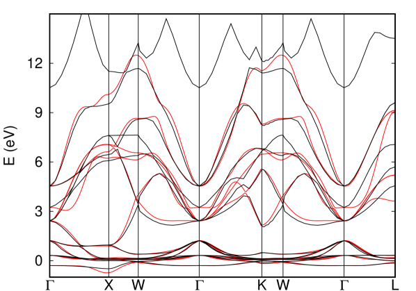
Figure 1: Electronic bands structure of NdN. Black lines correspond to DFT calculation and red lines are the result of the calculation with maximally localized Wannier functions. The Fermi level corresponds to zero energy.

A tight-binding electron model ($\hat{H}_{\text{orb}}+\hat{H}_{\text{t}}$) in the basis of maximally localized Wannier orbitals [83, 84] was derived from the DFT electronic bands around the Fermi level (see Appendix A.2). To reproduce the DFT bands with the tight-binding model (the red lines in Fig. 1), the Wannier functions of $4f$, $5d$ and $6s$ type had to be included, which was achieved by including the bands from the energy interval of 2$\div$12 eV (Fig. 1). The energies of the derived Wannier orbitals in one unit cell are given in Table 3 and the electron transfer parameters in Table S5 of SM [62]. Among the calculated DFT parameters, the $4f$ orbital energy levels are less accurate (Appendix B), and we do not use them in our analysis below.

The calculated band (Fig. 1) indicates a metallic ground state despite the fact that NdN is an insulator, whereas the nature of the solution does not give significant influence on $\hat{H}_{\text{t}}$ because the electron transfer parameters are basically determined by the overlap of the atomic orbitals of neighboring ions. The nature of the ground state is fully taken into consideration at the stage of the treatment of the entire model Hamiltonian. The derived transfer parameters are by several tens times smaller than Coulomb repulsion [63], clearly indicating that the ground state of our model Hamiltonian is deep in the correlated insulating phase. On this basis, the exchange interaction is derived by employing Anderson’s superexchange theory [45] in the next section.

III.3 Multipolar kinetic exchange interactions

(a)		(b)

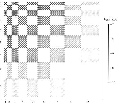
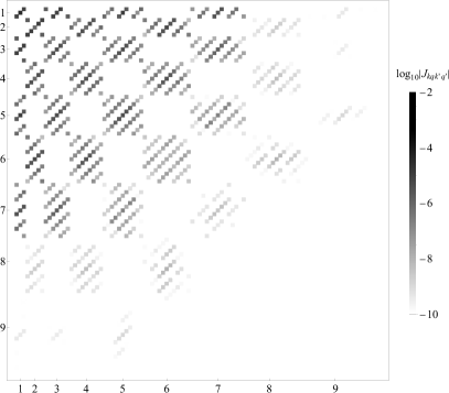
Figure 2: Magnitude of calculated exchange parameters $(\mathcal{J}_{fd})_{kqk^{\prime}q^{\prime}}$ in the logarithmic scale ($\log_{10}|(\mathcal{J}_{fd})_{kqk^{\prime}q^{\prime}}/\text{meV}|$) for allowed values of $kq$ and $k^{\prime}q^{\prime}$ for the nearest neighbor (a) and the next nearest neighbor (b) Nd pairs in NdN . The $\mathcal{J}_{fd})$ parameters presented here correspond to the tesseral tensor operators and are obtained by applying the transformation (24) to the corresponding parameters $\mathcal{I}_{fd}$ in Eq. (43). The ticks are for $kq$ in the increasing order of $k$ and $q$.

(a)		(b)

Figure 3: The spectrum of eigenstates of the exchange (a) and CF (b) parts of the $\hat{H}_{fd}$ operator (40) for the nearest neighbor Nd-Nd pair. The spectrum for a given value of $k$ corresponds to the case when terms up to $k$-th rank are included in the corresponding operator.

(a)		(b)

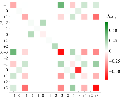
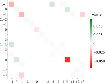
Figure 4: The exchange parameters $(\mathcal{J}_{fd})_{kqk^{\prime}q^{\prime}}$ between the $\Gamma_{8}$ multiplets of Nd³⁺ (in meV) for the nearest (a) and the next nearest (b) neighbors. The $\mathcal{J}$ parameters correspond to the tesseral representation of the downfolded exchange interaction between the $J$ multiplets of the coresponding Nd pairs with exchange parameters given in Fig. 2. The red and green squares correspond to ferromagnetic and antiferromagnetic contributions.

The multipolar magnetic interaction in NdN is investigated within the developed formalism in Sec. II using the input from the first-principles calculations. As we already mentioned, the whole family of the lanthanide nitrides LnN (Ln = Nd, Sm, Gd, Tb, Dy, Ho, Er) displays ferromagnetism with close Curie temperatures ($T_{\text{C}}$) despite strong differences in the structure of the lowest multiplets of Ln³⁺ ions. The latter have less than half-filled $f$ shells in NdN and SmN, exactly half-filled in GdN, and more than half-filled in DyN and HoN [55] implying large difference in the structure of their CF multiplets. The absence of the essential difference in $T_{\text{C}}$ among the LnN compounds suggests that the Goodenough’s contribution $\hat{H}_{fd}$ is dominant. In this subsection we analyse the Goodenough’s exchange contribution arising from $\hat{H}_{fd}$ in Eq. (41). The other kinetic exchange contributions and the dipolar magnetic interaction within Nd-Nd pairs are given in Sec. V of SM [62].

The exchange parameters $\mathcal{I}_{fd}$ (43) were calculated by substituting the first principles data (see Sec. A) and $U_{fd}$ into the the expressions derived in Sec. II.3.2. We have chosen the values $U_{fd}=3$ eV and 5 eV for the nearest and the next nearest neighbor Nd pairs, respectively, with which the experimental magnetic data are reproduced (see Sec. III.4). These values of $U_{fd}$ can be justified as follows. $U_{fd}$ is roughly estimated as $U_{fd}\approx(\epsilon_{d}-\epsilon_{f})+N(u_{fd}-u_{ff})-u^{\prime}$, where $N=3$ is the number of $4f$ electrons in Nd³⁺. The DFT values of the orbital energy gaps $(\epsilon_{d}-\epsilon_{f})$ between the $5d$ and the $4f$ are ca 4.3-7.6 eV (Table 3). The intra atomic Coulomb repulsion $u_{fd}$ is smaller than $u_{ff}\approx$ 5-7 eV [63] because of the diffuseness of the $5d$ orbitals. Indeed, the first-principles Slater-Condon $fd$ parameters were found several times smaller than the $ff$ ones (see Table S4 in SM [62]). The intersite classical Coulomb repulsion in vacuum is estimated 4 eV for the nearest neighbors and 2.8 eV for the next nearest neighbors, which are reduced few times by the screening effects. With these estimates, $U_{fd}$ amounts to 4-6 eV or less. All components of the calculated $\mathcal{J}_{fd}$ are shown in Fig. 2. The parameters corresponding to other exchange contributions are given in Figs. S3-S6 of SM [62].

It is easily seen that the range of possible ranks for nonzero exchange parameters (48) is satisfied in the plots of Fig. 2. The maximum rank becomes 9 ($=2J$) due to the ligand-field splitting of the $5d$ orbital levels at Nd [see Eq. (48)] . It emerges also that $\mathcal{J}_{fd}$ are zero whenever the ranks $k_{i}$ and $k_{j}$ are of different parity, i.e., when Eq. (37) is not fulfilled. Figure 2 shows that actually there are more cases of $(\mathcal{J}_{fd})_{k_{i}q_{i}k_{j}q_{j}}=0$ than those required by the parity of the ranks $k_{i}$ and $k_{j}$, which is explained by the spatial symmetry of the interacting ion pair (see for details Sec. V.A.1 in SM [62]). Furthermore, the nearest neighbor pairs have two-fold rotational symmetry, which gives an additional condition for nonzero $(\mathcal{J}_{fd})_{k_{i}q_{i}k_{j}q_{j}}$ that $q_{i}+q_{j}$ is even . The next nearest neighbor pairs have four-fold rotational symmetry, resulting in the condition for finite $(\mathcal{J}_{fd})_{k_{i}q_{i}k_{j}q_{j}}$ that $q_{i}+q_{j}$ is a multiple of 4. The derived interaction parameters are consistent with these symmetry requirements as well as with the constraints imposed by Eq. (48).

The multipolar interactions have non-negligible high-order terms. Fig. 2 shows that the lower rank exchange parameters tend to be larger (darker in the figure) than the higher rank ones, whereas a vast number of the high rank exchange coupling terms are nonzero, and their sum could result in non-negligible effects. The significance of the high-order terms was examined by calculating the exchange spectrum of the pairs within models gradually including higher ranked exchange interactions ($k=1,2,...9$) (Fig. 3). Besides, the kinetic contributions to the CF on Nd sites [the second and third terms in Eq. (40)] were analysed in the same manner. The exchange splitting shows that the first rank contribution ($k_{i}=k_{j}=1$) is dominant [Fig. 3 (a)]. This contribution differs from an isotropic Heisenberg exchange model $2\mathcal{J}_{\text{Heis}}\hat{\bm{J}}_{i}\cdot\hat{\bm{J}}_{j}$ by several additional terms . The calculated spectra display clear changes with the increase of the rank of added terms in the model up to $k=7$ for the exchange spectrum [Fig. 3 (a)] and $k=6$ for the CF spectrum on sites [Fig. 3 (b)]. This analysis suggests the importance of the high-order terms in $\hat{H}_{fd}$ for the magnetic properties of NdN and eventually other lanthanide nitrides.

The multipolar interactions also contribute to a scalar stabilization of the pair via the constant term $\mathcal{C}_{fd}$ (38) in $\hat{H}_{fd}$ (the first term in Eq. 40). The value of this term can amount as much as ca 10 times of the overall exchange splitting. The CF kinetic contribution described by the parameters (39) energetically is also significant [cf. Fig. 3 (b)]. Again, this CF contribution is stronger than the exchange one, which becomes evident when analysing the Goodenough’s exchange mechanism [60, 47]. Indeed, the expression for the exchange parameter corresponding to this mechanism contains an additional quenching factor $J_{\text{H}}/(U^{\prime}+\Delta_{fd})$ compared to the destabilization energy of $4f$ orbitals due to $f$-$d$ hybridization, $\approx t^{2}/(U^{\prime}+\Delta_{fd})$, where $t$, $\Delta_{fd}$, $U^{\prime}$ and $J_{\text{H}}$ are the electron transfer parameter, the energy gap between the $4f$ and $5d$ orbitals, and intrasite Coulomb and Hund couplings, respectively.

The negligible effect of magnetic dipolar interaction in NdN (and probably in other lanthanide nitrides) is in sharp contrast with its dominant contribution to the exchange interaction in many polynuclear lanthanide complexes [88]. The Ln ions are usually found in a low-symmetric environment favoring axial CF components w.r.t. some quantization axis which, at its turn, stabilize a CF multiplet with a maximal projection of magnetic moment on this axis [89]. Thus, in most dysprosium complexes the saturated magnetic moment at Dy³⁺ is $\approx$ 10 $\mu_{B}$ (being, of cause, highly anisotropic). Given the obtained magnetic moment on Nd³⁺ in NdN of 2.2 $\mu_{B}$, the dipolar magnetic interaction in the former is expected to be $\approx$ 20 times larger than in Nd for equal separation between Ln ions.

The evaluated exchange interaction suggests that the ferromagnetic order of NdN is of multipolar type. To obtain further physical insight, the exchange model was projected into the space of the ground $\Gamma_{8}$ multiplets, and transformed into the tesseral tensor form. The derived $\Gamma_{8}$ model shows that the strength of the nearest neighbor interaction is about one order of magnitude stronger than that of the next nearest neighbour one (Fig. 4). The interactions contain both ferro- (red) and antiferromultipolar (green) contributions, the ferromagnetic contributions being overall dominant. In particular, the interactions between octupole moments ($k=3$) are found to be the strongest. One may conclude that the exchange interaction is of ferro-octupolar type.

We have derived the multipolar exchange parameters by combining the DFT data and formula (43) rather than using other DFT based approaches because the applicability of the existing methods largely differs from that of the present method. The exchange interaction parameters have been often derived from the DFT band states by using Green’s function based approach [90], which is implemented in e.g. TB2J [91]. The approach uses one-particle Green’s function constructed on top of the DFT band structure, which naturally is suitable for the description of the systems that can be well described by band states: Simple magnetic metals (Fe, Ni, Co) and alloys, and some correlated insulators SrMnO₃, BiFeO₃ and La₂CuO₄ which could be well described within DFT+U method with spin polarization. In these systems, the multiplet electronic structures would not play significant role. On the other hand, it is difficult to utilize the Green’s function based method to study the multipolar exchange interactions of the compounds containing heavy transition metal, lanthanide, and actinide ions because in the latter systems explicit consideration of multiplet electronic structure is required.

III.4 Magnetic phase

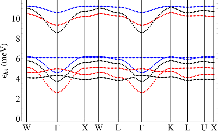
Figure 5: Low-energy part of the spin-wave dispersion (meV). The spectra in black, red and blue are derived with the full multipolar model, the $\Gamma_{8}$ model, and the Heisenberg model, respectively.

(a)		(b)	(c)
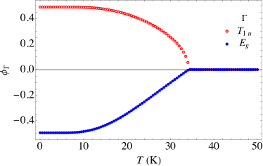
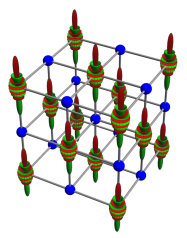
(d)		(e)

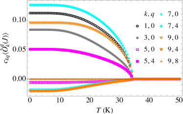
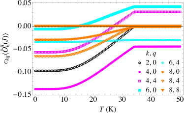
Figure 6: Primary ($T_{1u}$) and secondary ($E_{g}$) order parameters (a) and the largest components in the primary order parameters (b) and (c). Blue spheres are nitrogen atoms. The products of the expectation values $\langle\hat{O}_{k}^{q}\rangle$ and $c_{kq}$ for $\phi_{T_{1u}}$ (d) and $\phi_{E_{g}}$ (e), respectively.

With the derived multipolar interaction and CF at Nd sites, we next investigate the magnetic order of NdN within the mean-field approximation. In particular, the question on the origin of the ferromagnetism of NdN (and the entire family of lanthanide nitrides) is now addressed . To establish the correct nature of the multipolar magnetic phase, the primary order parameters should be first determined by employing the Landau theory for systems with multiple components.

The mean-field Hamiltonian for a single ion has the following form [Sec. VI.A.1 in SM [62]]:

$$\hat{H}_{\text{MF}}^{i} = C^{i}_{\text{MF}}+\hat{H}_{\text{CF}}^{i}+\sum_{k_{i}q_{i}}\hat{T}_{k_{i}q_{i}}^{i}\mathcal{F}_{k_{i}q_{i}}^{i},$$ (51)

where $C^{i}_{\text{MF}}$ is given by

$$C^{i}_{\text{MF}}=-\frac{1}{2}\sum_{k_{i}q_{i}}\langle\hat{T}_{k_{i}q_{i}}^{i}\rangle\mathcal{F}_{k_{i}q_{i}}^{i},$$ (52)

and the molecular field $\mathcal{F}_{kq}^{i}$ on site $i$ is defined as

$$\mathcal{F}_{k_{i}q_{i}}^{i} = \sideset{}{{}^{\prime}}{\sum}_{j(\neq i)}\sum_{k_{j}q_{j}}\left(\mathcal{I}^{ij}\right)_{k_{i}q_{i}k_{j}q_{j}}\langle\hat{T}_{k_{j}q_{j}}^{j}\rangle,$$ (53)

where $\langle\hat{T}_{k_{j}q_{j}}^{j}\rangle$ is the expectation value of the irreducible tensor operator (multipole moment) in thermal equilibrium. Diagonalizing Eq. (51), we obtain the eigenstates:

$$\hat{H}_{\text{MF}}|\mu\rangle=\epsilon_{\mu}|\mu\rangle,$$ (54)

where $\mu=0,1,...,9$ and $\epsilon_{0}\leq\epsilon_{1}\leq...\leq\epsilon_{9}$. The mean-field solutions were obtained self-consistently so that the $\langle\hat{T}_{k_{j}q_{j}}^{j}\rangle$ entering $\hat{H}_{\text{MF}}$ and the ones calculated with its eigenstates $|\mu\rangle$ coincide. The most stable magnetic order was found to be the ferromagnetic one with all magnetic moments aligned along one of the crystal axes, e.g., $c$, in full agreement with the neutron diffraction data [56].

The stability of the calculated ferromagnetic phase was confirmed by calculations of spin-wave dispersion. The magnon Hamiltonian was derived by employing the generalized Holstein-Primakoff transformation on top of the mean-field solutions [93, 20, 94] (Sec. V.A.2 in SM [62]). In this approach, each mean-field single-site state $|\mu\rangle$ is regarded as a one boson state, $\hat{b}_{\mu}^{\dagger}|0\rangle$, and the constraint on the number of magnon per site, $\sum_{\mu}\hat{b}_{\mu}^{\dagger}\hat{b}_{\mu}=1$, is imposed. Using the magnon creation $\hat{b}_{\mu}^{\dagger}$ and annihilation $\hat{b}_{\mu}$ operators, the tensor operators in $\hat{H}_{fd}$ are transformed, and the terms up to quadratic w.r.t. the magnon operators are retained. The obtained magnon Hamiltonian can be diagonalized by applying Bogoliubov-Valatin transformation [95, 96, 94]. The low-energy part of the calculated magnon band $\epsilon_{\bm{k}\lambda}$ shows the presence of the gap between the ground and the first excited states (the black lines in Fig. 5). Therefore, the stability of the mean-field ferromagnetic solution was confirmed [for entire spin-wave spectra, see Fig. S9 in SM [62]]. The ground state is stabilized by only 0.12 meV per site by including the zero point energy correction.

The obtained ferromagnetic phase is characterized by non-negligible high-order multipole moments. The order parameters were derived by employing Landau theory to mean-field Helmholtz free energy. Within this approach the second derivative of the free energy w.r.t. the primary order parameter becomes zero at the critical temperature. The Hessian of the mean-field free energy w.r.t. the multipole moments $\hat{T}_{kq}(\Gamma_{8})$ defined within the ground $\Gamma_{8}$ multiplet states was calculated. One of the eigenvalues of the Hessian becomes zero at $T=$ 29 K (the other is positive). Using the corresponding eigenvector, the primary $\phi_{T_{1u}}$ and the secondary $\phi_{E_{g}}$ order parameters were determined:

$$\phi_{T_{1u}} =0.454\langle\hat{T}_{10}(\Gamma_{8})\rangle+0.891\langle\hat{T}_{30}(\Gamma_{8})\rangle,$$ (55)

$$\phi_{E_{g}} =\langle\hat{T}_{20}(\Gamma_{8})\rangle.$$ (56)

The temperature evolution of the order parameters is shown in Fig. 6(a). These order parameters can be expanded through tesseral tensors $\hat{O}_{k}^{q}$, $\phi=\sum_{kq}c_{kq}\langle\hat{O}_{k}^{q}\rangle$ (24):

$$\phi_{T_{1u}}= -0.316\langle\hat{O}_{1}^{0}\rangle-0.313\langle\hat{O}_{3}^{0}\rangle+0.026\langle\hat{O}_{5}^{0}\rangle$$

$$+0.228\langle\hat{O}_{5}^{4}\rangle-0.257\langle\hat{O}_{7}^{0}\rangle+0.534\langle\hat{O}_{7}^{4}\rangle$$

$$-0.517\langle\hat{O}_{9}^{0}\rangle-0.355\langle\hat{O}_{9}^{4}\rangle+0.075\langle\hat{O}_{9}^{8}\rangle,$$ (57)

$$\phi_{E_{g}}= -0.397\langle\hat{O}_{2}^{0}\rangle-0.408\langle\hat{O}_{4}^{0}\rangle+0.483\langle\hat{O}_{4}^{4}\rangle$$

$$+0.336\langle\hat{O}_{6}^{0}\rangle+0.127\langle\hat{O}_{6}^{4}\rangle-0.308\langle\hat{O}_{8}^{0}\rangle$$

$$+0.462\langle\hat{O}_{8}^{4}\rangle+0.076\langle\hat{O}_{8}^{8}\rangle.$$ (58)

The expectation values of the components $(c_{kq}\langle\hat{O}_{k}^{q}\rangle)$ show that the largest contributions to the primary order parameter $\phi_{T_{1u}}$ come from $\hat{O}_{7}^{4}$, $\hat{O}_{1}^{0}$, and $\hat{O}_{9}^{0}$, and those to the secondary order parameter $\phi_{E_{g}}$ are also from almost all terms [Figs. 6 (d) and (e)]. The structures of the seventh and ninth moments are displayed in Figs. 6 (b) and (c). This analysis indicates that the ferromagnetic phase is of nontrivial multipolar type, mainly characterized by the tensor operators of ranks 7 and 9 along with the usual rank 1.

III.5 Magnetic and thermodynamic quantities

Table 2: Magnetic properties of NdN in the paramagnetic and ferromagnetic phases: the Curie-Weiss constant $T_{0}$, the effective magnetic moment ($M_{\text{eff}}$), the Curie temperature ($T_{\text{C}}$) and the saturated magnetic moment $M_{\text{sat}}$. The free ion data are $M_{\text{eff}}=g_{J}\sqrt{J(J+1)}$ and $M_{\text{sat}}=g_{J}J$ with $g_{J}=8/11$ and $J=9/2$.

	Paramagnetic		Ferromagnetic
	$T_{0}$ (K)	$M_{\text{eff}}$ ($\mu_{\text{B}}$)	$T_{\text{C}}$ (K)	$M_{\text{sat}}$ ($\mu_{\text{B}}$)
Theory (Present)	17.9	3.70	34.5	2.22
Free ion	-	3.62	-	3.27
Anton et al. [78]	$3\pm 4$	$3.6\pm 0.1$	$43\pm 1$	$1.0\pm 0.2$
Olcese [97]	10	3.63
Schobinger-Papamantellos et al. [56]				2.7
Busch et al. [98, 99]	24	3.65-4.00	32	3.1
Schumacher and Wallace [100]	15	3.70	35	2.15
Veyssie et al. [101]	19	Free ion	27.6	2.2

(a)	(b)
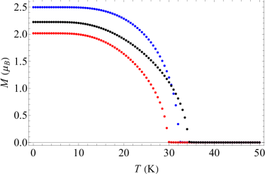
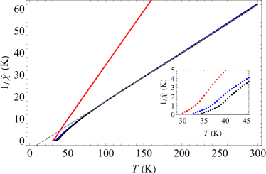
(c)	(d)

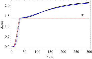
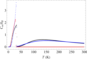
Figure 7: Magnetic and thermodynamic properties calculated with the full multipolar model (black), the model involving only the ground $\Gamma_{8}$ multiplet (red), and the Heisenberg exchange model (blue). (a) Magnetization $M$ ($\mu_{B}$), (b) magnetic susceptibility $\chi=(\mu_{\text{B}}^{2}/k_{\text{B}})\tilde{\chi}$, (c) magnetic entropy, (d) magnetic specific heat as functions of temperature $T$ (K). All quantities are in rapport to one unit cell.

The derived multipolar magnetic phase and its excitations are used for the calculation of magnetic and thermodynamic quantities of NdN [Figs. 6 and 7] (see also Sec. VI.B in SM [62]). These quantities include the magnetization $M$, magnetic susceptibility $\chi$, magnetic entropy $S_{m}$, and the magnetic part of specific heat.

The calculated saturated magnetic moment and the Curie temperature are close to the experimental data. The temperature dependence of the magnetic moment $M=\langle\hat{\mu}_{z}\rangle$ displays a second order phase transition at Curie point $T_{\text{C}}=$ 34.5 K [Fig. 7 (a)]. This agrees well with experimental data [100] (see Table 2.) . The saturated magnetic moment $M_{\text{sat}}$ at $T=0$ K is 2.22 $\mu_{\text{B}}$, which is slightly enhanced by the multipolar interaction compared with the post HF value (Sec. III.1). The enlargement of $M_{\text{sat}}$ w.r.t. the post HF value is explained by the hybridization of the ground and excited $\Gamma$ multiplets mainly due to the CF contribution in $\hat{H}_{fd}$ (40). In terms of the local $\Gamma$ multiplets [the eigenstates of the first-principles $\hat{H}_{\text{CF}}$ (49)], the lowest four mean-field solutions $|\mu\rangle$ ($\mu=$ 0-3) are written as

$$|0\rangle = 0.993\left|\Gamma_{8}^{(2)},-\frac{1}{2}\right\rangle+0.076\left|\Gamma_{6},-\frac{1}{2}\right\rangle$$

$$-0.087\left|\Gamma_{8}^{(1)},-\frac{1}{2}\right\rangle,$$

$$|1\rangle = 0.975\left|\Gamma_{8}^{(2)},+\frac{3}{2}\right\rangle-0.223\left|\Gamma_{8}^{(1)},+\frac{3}{2}\right\rangle,$$

$$|2\rangle = 1.000\left|\Gamma_{8}^{(2)},-\frac{3}{2}\right\rangle+0.018\left|\Gamma_{8}^{(1)},-\frac{3}{2}\right\rangle,$$

$$|3\rangle = 0.978\left|\Gamma_{8}^{(2)},+\frac{1}{2}\right\rangle+0.136\left|\Gamma_{6},+\frac{1}{2}\right\rangle$$ (59)

$$-0.157\left|\Gamma_{8}^{(1)},+\frac{1}{2}\right\rangle.$$

The admixture of the excited CF states in the four eigenstates (59) are 1.3, 5.0, 0.0 and 4.3 %, respectively, and the corresponding magnetic moments $\langle\hat{\mu}_{z}\rangle$ are 2.22, 0.67, 0.04 and $-$1.60 $\mu_{\text{B}}$.

The other calculated magnetic properties such as the Curie-Weiss constant and the effective magnetic moment also agree well with the experimental data derived from magnetic susceptibility. Using the calculated $M$, the magnetic susceptibility $\chi$ was calculated [Fig. 7 (b)]. The susceptibility in the high-temperature domain (80-300 K) was fit by the Curie-Weiss formula, from which the effective magnetic moment $M_{\text{eff}}$ and the Curie-Weiss constant $T_{0}$ were extracted, $M_{\text{eff}}=3.7\mu_{\text{B}}$ and $T_{0}=18$ K. $M_{\text{eff}}$ is close to the free ion value, suggesting that all CF multiplets contribute to the magnetic moment in the high-temperature domain. $T_{0}$ is obtained smaller than $T_{\text{C}}$, which is also in line with the experimental reports (Table 2). The calculated inverse magnetic susceptibility shows a ferrimagnetic-like nonlinear behavior around $35\lesssim T\lesssim 70$ K [Fig. 7 (a)], in agreement with experimental data [78]. In usual ferrimagnetic systems the magnetic moment of a unit cell drops at the transition temperature because the magnetic moments of different sublattices partially cancel each other below $T_{\text{C}}$, while they do not in the paramagnetic phase. Similar change in magnetic moment arises in NdN too albeit by a different mechanism: the thermal population of the excited CF multiplets with large magnetic moments enhances the $M_{\text{eff}}$ above $T_{\text{C}}$. The impact of the excited CF levels becomes visible when comparing the data with (the black lines) and without (the red lines) including them in the calculation (Fig. 7).

The calculated magnetic entropy $S_{\text{m}}$ is zero at $T=0$ K and rapidly grows as temperature rises [Fig. 7 (c)]. It reaches the value of $k_{\text{B}}\text{ln}4$ at $T=T_{\text{C}}$, which is the entropy from the ground $\Gamma_{8}$ quartet, and displays a kink. Above $T_{\text{C}}$, the entropy gradually increases. The magnetic part of the specific heat $C_{\text{m}}$ grows from $T=0$ K and displays a sharp peak at $T_{\text{C}}$ (Fig. 7 d). Above $T_{\text{C}}$, $C_{\text{m}}$ has a broad peak as expected from $S_{\text{m}}$. The temperature evolution of $S_{\text{m}}$ and $C_{\text{m}}$ above $T_{\text{C}}$ is explained by the thermal population of the excited CF multiplets, similarly to $M_{\text{eff}}$. The importance of the excited CF multiplets for the calculated properties becomes evident from a comparison with the results of the corresponding calculations in which they are not included [red lines in Figs. 7(c), (d)].

III.6 Fingerprint of multipolar ordering

The signs of multipolar character of the ferromagnetic phase appears in the magnon spectra. To evidence them, the magnon spectrum calculated within the multipolar exchange model was compared with the one calculated within the isotropic Heisenberg model, $2\mathcal{J}_{\text{Heis}}^{ij}\hat{\bm{J}}_{i}\cdot\hat{\bm{J}}_{j}$. The Heisenberg exchange parameters were chosen to match the overall exchange splitting given by the multipolar model [Fig. 3(a)], $\mathcal{J}_{\text{Heis}}=-3.51$ and $-0.28$ meV for the nearest and the next nearest neighbor pairs, respectively. The CF Hamiltonian was kept the same as in the multipolar calculations. Fig. 7 shows (blue lines) that the Heisenberg model gives similar behaviour of magnetic and thermodynamic quantities with the multipole model. Notable differences are seen in the low-energy part of the spin-wave spectrum (Fig. 5). Thus the Heisenberg magnon band (blue) at about 6 meV is flat, while the multipolar one (black) is not. Moreover, the two Heisenberg bands on X-W-L and K-L-U-X paths are quasi degenerate, while those of the multipolar model are largely split.

Hence the excitation spectra can give a straightforward information on the multipolar order and interactions, however, in the NdN they have not been experimentally investigated. In order to get insight into the multipolar order and to check the predictions given here experimental studies such as inelastic neutron scattering are most desired.

IV Conclusions

In this work, on the basis of explicitly correlated ab initio approaches and DFT calculations a first-principles microscopic theory of multipolar magnetic coupling between $J$-multiplets in $f$-electron magnetic insulators was developed. Besides conventional contributions to the exchange coupling, an important ingredient of the present theory is a complete first-principles description of Goodenough’s exchange mechanism, which is of primary importance for the magnetic coupling in lanthanide materials. The theory was applied to the investigation of multipolar exchange interaction and magnetic order in neodymium nitride. Despite the apparent simplicity of this material exhibiting a collinear ferromagnetism, our analysis reveal the multipolar nature of its magnetic order, described by primary and secondary order parameters and containing non-negligible $J$-tensorial contributions up to the ninth order. The first-principles theory reproduces well the known experimental data on its octupolar-ferromagnetic phase. We predict that the fingerprints of the multipolar order in this material can be found in the spin-wave dispersion and should be observable, e.g., in inelastic neutron scattering. The developed first principles framework for the calculation of multipolar exchange parameters can become an indispensable tool in future investigations of lanthanide and actinide based magnetic insulators.

Acknowledgement

N.I. was partly supported by the GOA program from KU Leuven and the scientific research grant R-143-000-A80-114 of the National University of Singapore during this project. Z.H. gratefully acknowledges funding by the China Scholarship Council. I.N. thanks the Theoretical and Computational Chemistry European Master Program (TCCM) for financial support. The computational resources and services used in this work were provided by the VSC (Flemish Supercomputer Center) funded by the Research Foundation - Flanders (FWO) and the Flemish Government - department EWI.

Appendix A Computational method

A.1 Post HF calculations

The CF states of embedded Nd³⁺ were calculated employing a post HF approach (CASSCF). To this end fragment calculations of NdN have been performed by cutting a mononuclear cluster from the experimental structure of NdN [97]. The cluster has $O_{h}$ symmetry and consists of a central Nd and 6 nearest neighbor N atoms which were treated fully quantum mechanically with atomic-natural orbital relativistic-correlation consistent-valence quadruple zeta polarization (ANO-RCC-VQZP) basis, and neighboring 32 N and 42 Nd with ANO-RCC-minimal basis (MB) and ab initio embedding model potential [103], respectively. This cluster was surrounded by 648 point charges. For the calculations of multiplet structures, CASSCF method and subsequently spin-orbit restricted-active-space state interaction (SO-RASSI) approach [40] were employed. The CASSCF/SO-RASSI calculations of the cluster were performed with 3 electrons in 14 active orbitals ($4f$ and $5f$ types) . The atomic two-electron integrals were computed using Cholesky decomposition with a threshold of $1.0\times 10^{-9}$ $E_{h}$. The inversion symmetry was used. All the calculations were carried out with Molcas 8.2 package [105].

Based on the calculated low-energy SO-RASSI states, the CF Hamiltonian was derived. By a unitary transformation of the lowest 10 SO-RASSI states, the $J$-pseudospin states ($J=9/2$) were uniquely defined [79, 42, 43]. With the obtained $J$ pseudospin states and the energy spectrum, the first-principles based CF model [42, 43, 39] was derived employing the algorithm developed for $O_{h}$ systems [80]. The CF parameters $\mathcal{B}_{kq}$ were mapped into an effective $4f$ orbital model to extract the effective orbital energy levels as in Ref. [106].

The post HF approach was also used for isolated Nd ions to derive the Coulomb interaction (Slater-Condon) parameters and spin-orbit couplings. The CASSCF calculations of isolated Ndⁿ⁺ ions $(n=$2-4) were performed for all possible spin multiplicities to determine the $LS$-term energies. The calculated energies were fit to the electrostatic Hamiltonian for the $f^{N}$ ion tabulated in Ref. [75] or those for the $f^{N}d^{1}$ or $f^{N}s^{1}$ ions [107] (see Sec. II.D in SM [62]). The eigenstates of the electrostatic Hamiltonian give the relation between the symmetrized $LS$ states [75] and the $LS$-term states, with which the c.f.p. were transformed. The $J$ multiplet states were obtained by performing the SO-RASSI calculations on top of the CASSCF states. By fitting the SO-RASSI levels to the model atomic Hamiltonian, the spin-orbit parameters (4) were determined (see Sec. II. E in Ref. [62]).

A.2 DFT band calculations

The band calculations were performed with full potential linearized augmented plane wave (LAPW) approach implemented in Wien2k [108] allowing an accurate treatment of heavy elements. The generalized gradient approximation (GGA) functional parameterized by Perdew, Burke, and Ernzerhof [109] were employed. For the LAPW basis functions in interstitial region, a plane wave cut-off of $k_{\text{max}}=8.5/R_{\text{mt}}$ was chosen, where $R_{\text{mt}}$ is the smallest atomic muffin-tin radius in the unit cell. The muffin-tin radii were set to 2.50 $a_{0}$ for Nd and 2.11 $a_{0}$ for N, where $a_{0}$ is the Bohr radius. A $6\times 6\times 6$ $k$ point sampling for Brillouin zone integral was used in the self-consistent calculation.

Based on the obtained band structure, maximally localized Wannier functions [83, 84] were derived using Wien2wannier [110], for which a $3\times 3\times 3$ $k$ sampling was employed. In the present case the target bands entangle with other irrelevant bands, so that to derive the Wannier functions the strategy used in Ref. [111] was employed: This consists with including all the bands within the energy window of [$-$0.5, 12.5] eV with an inner energy window [$-$0.5, 10] eV (the Fermi level is set to zero of energy), and projecting the target bands onto $4f$, $5d$ and $6s$ orbitals of Nd atom. The symmetry of the obtained Wannier functions was slightly lowered, and hence they were symmetrized by comparing the obtained tight-binding model with the Slater-Koster model [112, 113].

Table 3: Orbital energy levels extracted from the post HF and band calculations (eV). The irreducible representations (irrep.) of the $O_{h}$ group are shown in the parenthesis. The lowest post HF orbital energy level is set at zero energy.

$nl$	irrep.	Post HF	DFT
$4f$	$a_{2u}$	0	0.0297
	$t_{1u}$	0.0941	0.3175
	$t_{2u}$	0.0191	0.2793
$5d$	$t_{2g}$	-	4.3216
	$e_{g}$	-	7.5913
$6s$	$a_{1g}$	-	8.6130

Appendix B Orbital energy levels

The validity of the $4f$ orbital levels from ab initio and DFT calculations can be checked by making use of a relaiton between the CF levels and $4f$ orbital levels. Assuming that the CF originates from single electron potential, the CF Hamiltonian $\hat{H}_{\text{CF}}$ (18) can be mapped into a single-electron model $\hat{H}_{\text{loc}}$ (2) and vice versa (see Sec. II.B in SM [62]). The calculated effective orbital energy levels are given in Table 3.

The $4f$ orbital energy levels derived from the post HF and DFT calculations differ much. The ab initio $4f$ orbital splitting is estimated to be only 94 meV, which is much smaller than the other intrasite interactions (2). The order of the CF split $4f$ orbitals are consistent with the post HF data, whereas the quantities are a few times larger than the latter. By using the same relation, we found that the DFT $4f$ orbital levels gives qualitatively wrong CF levels: The calculated DFT CF levels are 0 ($\Gamma_{6}$), 86 ($\Gamma_{8}$) and 120 ($\Gamma_{8}$) meV. The discrepancy between DFT data and post HF calculations could be explained by an exaggerated hybridization of the $4f$ orbitals with the ligand environment in the DFT calculations at GGA level.

References

- Santini et al. [2009] P. Santini, S. Carretta, G. Amoretti, R. Caciuffo, N. Magnani, and G. H. Lander, Multipolar interactions in -electron systems: The paradigm of actinide dioxides, Rev. Mod. Phys. 81, 807 (2009).
- Kuramoto et al. [2009] Y. Kuramoto, H. Kusunose, and A. Kiss, Multipole orders and fluctuations in strongly correlated electron systems, J. Phys. Soc. Jpn. 78, 072001 (2009).
- Onimaru and Kusunose [2016] T. Onimaru and H. Kusunose, Exotic Quadrupolar Phenomena in Non-Kramers Doublet Systems - The Cases of PrT2Zn20 (T = Ir, Rh) and PrT2Al20 (T = V, Ti) -, J. Phys. Soc. Jpn. 85, 082002 (2016).
- Suzuki et al. [2018] M.-T. Suzuki, H. Ikeda, and P. M. Oppeneer, First-principles Theory of Magnetic Multipoles in Condensed Matter Systems, J. Phys. Soc. Jpn. 87, 041008 (2018).
- Rau and Gingras [2019] J. G. Rau and M. J. Gingras, Frustrated Quantum Rare-Earth Pyrochlores, Annu. Rev. Condens. Matter Phys. 10, 357 (2019).
- Mydosh et al. [2020] J. A. Mydosh, P. M. Oppeneer, and P. S. Riseborough, Hidden order and beyond: an experimental—theoretical overview of the multifaceted behavior of URu2Si2, J. Phys.: Condens. Matter 32, 143002 (2020).
- Shiina et al. [1997] R. Shiina, H. Shiba, and P. Thalmeier, Magnetic-Field Effects on Quadrupolar Ordering in a -Quartet System CeB6, J. Phys. Soc. Jpn. 66, 1741 (1997).
- Mironov et al. [2003a] V. S. Mironov, L. F. Chibotaru, and A. Ceulemans, First-order Phase Transition in UO2: The Interplay of the - Superexchange Interaction and Jahn–Teller Effect, in Adv. Quant. Chem., Adv. Quant. Chem., Vol. 44 (Academic Press, 2003) pp. 599 – 616.
- Santini et al. [2006] P. Santini, S. Carretta, N. Magnani, G. Amoretti, and R. Caciuffo, Hidden Order and Low-Energy Excitations in , Phys. Rev. Lett. 97, 207203 (2006).
- Kusunose [2008] H. Kusunose, Description of Multipole in f-Electron Systems, J. Phys. Soc. Jpn. 77, 064710 (2008).
- Rau and Gingras [2015] J. G. Rau and M. J. P. Gingras, Magnitude of quantum effects in classical spin ices, Phys. Rev. B 92, 144417 (2015).
- Watanabe and Yanase [2018] H. Watanabe and Y. Yanase, Group-theoretical classification of multipole order: Emergent responses and candidate materials, Phys. Rev. B 98, 245129 (2018).
- Rau and Gingras [2018] J. G. Rau and M. J. P. Gingras, Frustration and anisotropic exchange in ytterbium magnets with edge-shared octahedra, Phys. Rev. B 98, 054408 (2018).
- Dudarev et al. [2019] S. L. Dudarev, P. Liu, D. A. Andersson, C. R. Stanek, T. Ozaki, and C. Franchini, Parametrization of for noncollinear magnetic configurations: Multipolar magnetism in , Phys. Rev. Materials 3, 083802 (2019).
- Pourovskii and Khmelevskyi [2019] L. V. Pourovskii and S. Khmelevskyi, Quadrupolar superexchange interactions, multipolar order, and magnetic phase transition in , Phys. Rev. B 99, 094439 (2019).
- Hallas et al. [2020] A. M. Hallas, W. Jin, J. Gaudet, E. M. Tonita, D. Pomaranski, C. R. C. Buhariwalla, M. Tachibana, N. P. Butch, S. Calder, M. B. Stone, G. M. Luke, C. R. Wiebe, J. B. Kycia, M. J. P. Gingras, and B. D. Gaulin, Intertwined magnetic dipolar and electric quadrupolar correlations in the pyrochlore Tb2Ge2O7 (2020), arXiv:2009.05036 [cond-mat.str-el] .
- Gritsenko et al. [2020] Y. Gritsenko, S. Mombetsu, P. T. Cong, T. Stöter, E. L. Green, C. S. Mejia, J. Wosnitza, M. Ruminy, T. Fennell, A. A. Zvyagin, S. Zherlitsyn, and M. Kenzelmann, Changes in elastic moduli as evidence for quadrupolar ordering in the rare-earth frustrated magnet Tb2Ti2O7, Phys. Rev. B 102, 060403 (2020).
- Sibille et al. [2020] R. Sibille, N. Gauthier, E. Lhotel, V. Porée, V. Pomjakushin, R. A. Ewings, T. G. Perring, J. Ollivier, A. Wildes, C. Ritter, T. C. Hansen, D. A. Keen, G. J. Nilsen, L. Keller, S. Petit, and T. Fennell, A quantum liquid of magnetic octupoles on the pyrochlore lattice, Nat. Phys. 16, 546 (2020).
- Pourovskii and Khmelevskyi [2021] L. V. Pourovskii and S. Khmelevskyi, Hidden order and multipolar exchange striction in a correlated -electron system, Proc. Nat. Acad. Sci. 118, e2025317118 (2021).
- Chen et al. [2010] G. Chen, R. Pereira, and L. Balents, Exotic phases induced by strong spin-orbit coupling in ordered double perovskites, Phys. Rev. B 82, 174440 (2010).
- Chen and Balents [2011] G. Chen and L. Balents, Spin-orbit coupling in ordered double perovskites, Phys. Rev. B 84, 094420 (2011).
- Romhányi et al. [2017] J. Romhányi, L. Balents, and G. Jackeli, Spin-Orbit Dimers and Noncollinear Phases in Cubic Double Perovskites, Phys. Rev. Lett. 118, 217202 (2017).
- Ishikawa et al. [2019] H. Ishikawa, T. Takayama, R. K. Kremer, J. Nuss, R. Dinnebier, K. Kitagawa, K. Ishii, and H. Takagi, Ordering of hidden multipoles in spin-orbit entangled ta chlorides, Phys. Rev. B 100, 045142 (2019).
- Maharaj et al. [2020] D. D. Maharaj, G. Sala, M. B. Stone, E. Kermarrec, C. Ritter, F. Fauth, C. A. Marjerrison, J. E. Greedan, A. Paramekanti, and B. D. Gaulin, Octupolar versus Néel Order in Cubic Double Perovskites, Phys. Rev. Lett. 124, 087206 (2020).
- Hirai et al. [2020] D. Hirai, H. Sagayama, S. Gao, H. Ohsumi, G. Chen, T.-h. Arima, and Z. Hiroi, Detection of multipolar orders in the spin-orbit-coupled Mott insulator , Phys. Rev. Research 2, 022063 (2020).
- Wahab et al. [2021] D. A. Wahab, M. Augustin, S. M. Valero, W. Kuang, S. Jenkins, E. Coronado, I. V. Grigorieva, I. J. Vera-Marun, E. Navarro-Moratalla, R. F. L. Evans, K. S. Novoselov, and E. J. G. Santos, Quantum Rescaling, Domain Metastability, and Hybrid Domain-Walls in 2D CrI3 Magnets, Adv. Mater. 33, 2004138 (2021).
- Yamamoto et al. [2020] D. Yamamoto, C. Suzuki, G. Marmorini, S. Okazaki, and N. Furukawa, Quantum and Thermal Phase Transitions of the Triangular SU(3) Heisenberg Model under Magnetic Fields, Phys. Rev. Lett. 125, 057204 (2020).
- Kaplan and Vekhter [1995] M. D. Kaplan and B. G. Vekhter, Cooperative Phenomena in Jahn-Teller Crystals (Plenum Press, New York and London, 1995).
- Levy [1964] P. M. Levy, Rare-Earth-Iron Exchange Interaction in the Garnets. I. Hamiltonian for Anisotropic Exchange Interaction, Phys. Rev. 135, A155 (1964).
- Levy [1966] P. M. Levy, Rare-Earth-Iron Exchange Interaction in the Garnets. II. Exchange Potential for Ytterbium, Phys. Rev. 147, 311 (1966).
- Hartmann-Boutron [1968] F. Hartmann-Boutron, Interactions de superéchange en présence de dégénérescence orbitale et de couplage spin-orbite, J. Phys. France 29, 212 (1968).
- Elliott and Thorpe [1968] R. J. Elliott and M. F. Thorpe, Orbital Effects on Exchange Interactions, J. Appl. Phys. 39, 802 (1968).
- Baker et al. [1968] J. M. Baker, R. J. Birgeneau, M. T. Hutchings, and J. D. Riley, High-Degree Exchange Interaction Between Rare-Earth Ions, Phys. Rev. Lett. 21, 620 (1968).
- Birgeneau et al. [1969] R. J. Birgeneau, M. T. Hutchings, J. M. Baker, and J. D. Riley, High-Degree Electrostatic and Exchange Interactions in Rare-Earth Compounds, J. Appl. Phys. 40, 1070 (1969).
- Mironov et al. [2003b] V. S. Mironov, L. F. Chibotaru, and A. Ceulemans, Exchange interaction in the mixed dimer: The origin of a strong exchange anisotropy, Phys. Rev. B 67, 014424 (2003b).
- Iwahara and Chibotaru [2015] N. Iwahara and L. F. Chibotaru, Exchange interaction between multiplets, Phys. Rev. B 91, 174438 (2015).
- Vieru et al. [2016] V. Vieru, N. Iwahara, L. Ungur, and L. F. Chibotaru, Giant exchange interaction in mixed lanthanides, Sci. Rep. 6, 24046 (2016).
- Nguyen and Ungur [2021] G. T. Nguyen and L. Ungur, Understanding the magnetization blocking mechanism in N-radical-bridged dilanthanide single-molecule magnets, Phys. Chem. Chem. Phys. , (2021).
- Ungur and Chibotaru [2017] L. Ungur and L. F. Chibotaru, Ab Initio Crystal Field for Lanthanides, Chem. Eur. J. 23, 3708 (2017).
- Roos et al. [2016] B. O. Roos, R. Lindh, P.-A. Malmqvist, V. Veryazov, and P.-O. Widmark, Multiconfigurational Quantum Chemistry (John Wiley & Sons, Inc., New Jersey, 2016).
- Aquilante et al. [2020] F. Aquilante, J. Autschbach, A. Baiardi, S. Battaglia, V. A. Borin, L. F. Chibotaru, I. Conti, L. De Vico, M. Delcey, I. Fdez. Galván, N. Ferré, L. Freitag, M. Garavelli, X. Gong, S. Knecht, E. D. Larsson, R. Lindh, M. Lundberg, P. Å. Malmqvist, A. Nenov, J. Norell, M. Odelius, M. Olivucci, T. B. Pedersen, L. Pedraza-González, Q. M. Phung, K. Pierloot, M. Reiher, I. Schapiro, J. Segarra-Martí, F. Segatta, L. Seijo, S. Sen, D.-C. Sergentu, C. J. Stein, L. Ungur, M. Vacher, A. Valentini, and V. Veryazov, Modern quantum chemistry with [Open]Molcas, J. Chem. Phys. 152, 214117 (2020).
- Chibotaru and Ungur [2012] L. F. Chibotaru and L. Ungur, Ab initio calculation of anisotropic magnetic properties of complexes. I. Unique definition of pseudospin Hamiltonians and their derivation, J. Chem. Phys. 137, 064112 (2012).
- Chibotaru [2013] L. F. Chibotaru, Ab Initio Methodology for Pseudospin Hamiltonians of Anisotropic Magnetic Complexes, in Adv. Chem. Phys. (John Wiley & Sons, Ltd, 2013) Chap. 6, pp. 397–519.
- Imada et al. [1998] M. Imada, A. Fujimori, and Y. Tokura, Metal-insulator transitions, Rev. Mod. Phys. 70, 1039 (1998).
- Anderson [1959] P. W. Anderson, New Approach to the Theory of Superexchange Interactions, Phys. Rev. 115, 2 (1959).
- Kanamori [1959] J. Kanamori, Superexchange interaction and symmetry properties of electron orbitals, J. Phys. Chem. Solids 10, 87 (1959).
- Goodenough [1963] J. B. Goodenough, Magnetism and the Chemical Bond (Interscience, New York, 1963).
- Huang et al. [2020] Z. Huang, D. Liu, A. Mansikkamäki, V. Vieru, N. Iwahara, and L. F. Chibotaru, Ferromagnetic kinetic exchange interaction in magnetic insulators, Phys. Rev. Research 2, 033430 (2020).
- Vieru et al. [2013] V. Vieru, L. Ungur, and L. F. Chibotaru, Key Role of Frustration in Suppression of Magnetization Blocking in Single-Molecule Magnets, J. Phys. Chem. Lett. 4, 3565 (2013).
- Westerström et al. [2014] R. Westerström, J. Dreiser, C. Piamonteze, M. Muntwiler, S. Weyeneth, K. Krämer, S.-X. Liu, S. Decurtins, A. Popov, S. Yang, L. Dunsch, and T. Greber, Tunneling, remanence, and frustration in dysprosium-based endohedral single-molecule magnets, Phys. Rev. B 89, 060406 (2014).
- Rinehart et al. [2011a] J. D. Rinehart, M. Fang, W. J. Evans, and J. R. Long, Strong exchange and magnetic blocking in N-radical-bridged lanthanide complexes, Nat. Chem. 3, 538 (2011a).
- Rinehart et al. [2011b] J. D. Rinehart, M. Fang, W. J. Evans, and J. R. Long, A N Radical-Bridged Terbium Complex Exhibiting Magnetic Hysteresis at 14 K, J. Am. Chem. Soc. 133, 14236 (2011b).
- Demir et al. [2017] S. Demir, M. I. Gonzalez, L. E. Darago, W. J. Evans, and J. R. Long, Giant coercivity and high magnetic blocking temperatures for N radical-bridged dilanthanide complexes upon ligand dissociation, Nat. Commun. 8, 2144 (2017).
- Goodwin et al. [2020] C. A. P. Goodwin, B. L. L. Réant, G. F. Vettese, J. G. C. Kragskow, M. J. Giansiracusa, I. M. DiMucci, K. M. Lancaster, D. P. Mills, and S. Sproules, Heteroleptic Samarium(III) Chalcogenide Complexes: Opportunities for Giant Exchange Coupling in Bridging - and -Radical Lanthanide Dichalcogenides, Inorg. Chem. 59, 7571 (2020).
- Natali et al. [2013] F. Natali, B. J. Ruck, N. O. V. Plank, H. J. Trodahl, S. Granville, C. Meyer, and W. R. L. Lambrecht, Rare-earth mononitrides, Prog. Mater. Sci. 58, 1316 (2013).