Fast Cooling of Trapped Ion in Strong Sideband Coupling Regime

Abstract

Trapped ion in the Lamb-Dicke regime with the Lamb-Dicke parameter $\eta\ll 1$ can be cooled down to its motional ground state using sideband cooling. Standard sideband cooling works in the weak sideband coupling limit, where the sideband coupling strength is small compared to the natural linewidth $\gamma$ of the internal excited state, with a cooling rate much less than $\gamma$. Here we consider cooling schemes in the strong sideband coupling regime, where the sideband coupling strength is comparable or even greater than $\gamma$. We derive analytic expressions for the cooling rate and the average occupation of the motional steady state in this regime, based on which we show that one can reach a cooling rate which is proportional to $\gamma$, while at the same time the steady state occupation increases by a correction term proportional to $\eta^{2}$ compared to the weak sideband coupling limit. We demonstrate with numerical simulations that our analytic expressions faithfully recover the exact dynamics in the strong sideband coupling regime.

I Introduction

Trapped ions display rich physical phenomena due to its high degree of controllability and abundant degrees of freedom. In the context of quantum simulations, trapped ions can be used to realize quantum spin systems Porras and Cirac (2004a), the Bose-Hubbard chain Porras and Cirac (2004b), the Jaynes-Cummings model Leibfried et al. (2003) with tunable interactions, as well as to study energy and particle transport far from equilibrium Bermúdez et al. (2013); Ruiz et al. (2014); Ramm et al. (2014); Guo et al. (2015); Guo and Poletti (2016, 2017a, 2017b, 2018). Trapped ions system is also a promising candidate to build quantum computers Lanyon et al. (2011); Kielpinski et al. (2002), where the internal degrees of freedom are used to encode the qubits and the external (motional) degrees of freedom are used to induce effective couplings between those qubits Cirac and Zoller (1995). The motional degrees of freedom of trapped ions play a central role in realizing all the above systems or schemes, being used either directly or indirectly. Particularly, in the context of quantum computing, cooling the motional degrees of freedom down to their ground states is a central step for coherent manipulation of the quantum state Wineland et al. (1998).

Sideband cooling is one of the first and still widely used cooling scheme Diedrich et al. (1989); Monroe et al. (1995); Roos et al. (1999). The key ideas of sideband cooling are summarized as follows, which are also helpful for understanding other cooling schemes using static lasers. First we assume that an ion with two internal states, say a metastable ground state $|g\rangle$ and an unstable excited state $|e\rangle$ with a lifetime $\tau=1/\gamma$ ($\gamma$ is the linewidth and we have set $\hbar=1$), is trapped in a way that the motional degree of freedom of the ion is described by a harmonic oscillator with equidistant energy levels $|n\rangle$ of energies $(n+\frac{1}{2})\nu$, where $\nu$ is the trap frequency. A laser with Rabi frequency $\Omega$ is then applied onto the ion with detuning $\Delta$ which, in the first order of the Lamb-Dicke (LD) parameter $\eta$, induces a carrier transition $|g,n\rangle\leftrightarrow|e,n\rangle$ with strength $\Omega$, a red sideband $|g,n\rangle\leftrightarrow|e,n-1\rangle$ and a blue sideband $|g,n\rangle\leftrightarrow|e,n+1\rangle$ with strengths $\eta\Omega\sqrt{n}$ and $\eta\Omega\sqrt{n+1}$, respectively. For this first order picture to be valid, the following conditions need to be satisfied: 1) the Lamb-Dicke condition $\eta\ll 1$, which requires the oscillations of the trapped ion to be much smaller than the wave length of the cooling laser, 2) resolved sideband condition, which requires $\eta\Omega,\gamma\ll\nu$. The laser is often tuned to red sideband resonance, namely $\Delta=-\nu$, such that the blue sideband is far-detuned compared to the red sideband and can often be neglected. The red sideband together with the natural decay $|e\rangle\rightarrow|g\rangle$ form a dissipative cascade Cohen-Tannoudji et al. (1998) which makes the cooling possible. Most existing cooling schemes works in the weak sideband coupling (WSC) regime, which requires additionally $\eta\Omega\ll\gamma$, so that the states $|e,n-1\rangle$ decay to $|g,n-1\rangle$ immediately once pumped up from $|g,n\rangle$ by the red sideband. As a result the states $|e,n-1\rangle$ can be adiabatically eliminated from the cascade and one gets an effective decay from $|g,n\rangle$ to $|g,n-1\rangle$ with a rate

$$W_{{\rm WSC}}\propto\frac{\eta^{2}\Omega^{2}}{\gamma}.$$ (1)

The weak sideband coupling condition thus sets a cooling rate which is much less than the natural linewidth $\gamma$.

Subsequent proposals using static lasers mainly aim to improve the quality of the steady state by suppressing the heating effects due to the carrier transition or the blue sideband Cirac et al. (1992); Morigi et al. (2000); Morigi (2003); Retzker and Plenio (2007), or both of them Evers and Keitel (2004); Cerrillo et al. (2010, 2018); Albrecht et al. (2011); Zhang et al. (2012, 2014); Lu et al. (2015), by adding more lasers as well as more internal energy levels. As an outstanding example, cooling by electromagnetically induced transparency (EIT) eliminates the carrier transition Morigi et al. (2000); Morigi (2003), which has been demonstrated in various experiments due to its simplicity and effectiveness Roos et al. (2000); Lin et al. (2013); Kampschulte et al. (2014); Lechner et al. (2016); Scharnhorst et al. (2018); Jordan et al. (2019); Feng et al. (2020); Qiao et al. (2020). Quantum control has also been applied in recent years to numerically find an optimal sequence of pulsed lasers which drives the trapped ion towards its motional ground state Machnes et al. (2010). An advantage of cooling with pulsed lasers is that the lasers could often be tuned such that fast cooling can be achieved compared to sideband cooling, while the drawbacks are that the time-dependence of the lasers adds more difficulty for the experimental implementation, and that the initial motional state is often required to be known precisely in such schemes.

In this work, we focus on cooling schemes using static lasers. In particular, we aim to improve the cooling rate set by Eq.(1), which is essential in all applications to reduce the associated dead time Scharnhorst et al. (2018). For this goal, we consider cooling schemes in the strong sideband coupling (SSC) regime, where $\eta\Omega$ is comparable with or even larger than $\gamma$, namely $\eta\Omega\geq\gamma$. Eq.(1) fails in the SSC regime, which effect has been observed both numerically Albrecht et al. (2011); Zhang et al. (2014); Lu et al. (2015); Cerrillo et al. (2018) and experimentally Scharnhorst et al. (2018). In particular, we consider both the standing wave sideband cooling and the EIT cooling schemes in the SSC regime such that the heating effects due to the carrier transitions are suppressed. In both cases, we show analytically and numerically that we can reach a cooling rate $W_{\textrm{SSC}}\propto\gamma$ in the SSC regime, independent of the sideband coupling strength $\eta\Omega$. The price to pay is a correction term to the steady state occupation of the motional degree of freedom which is proportional to $\eta^{2}$. This paper is organized as follows. We first consider the standing wave sideband cooling in the SSC regime in Sec. II. We derive analytic expressions for the dynamics of the average occupation of the motional state as well as its steady state value, which are verified by comparison to exact numerical results. In Sec.III, we further generalize those expressions to EIT cooling in the SSC regime. We conclude in Sec. IV.

II Standing wave sideband cooling in the SSC regime

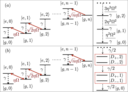
Figure 1: (a) Standing wave sideband cooling in the weak sideband coupling regime. The laser resonantly couples $|g,n\rangle$ to $|e,n-1\rangle$, which then decays to $|g,n-1\rangle$ immediately without oscillating back into $|g,n\rangle$. Therefore the time to stay in the state $|e,n-1\rangle$ is negligible and $|e,n-1\rangle$ is adiabatically eliminated, resulting in an effective decay from $|g,n\rangle$ to $|g,n-1\rangle$ as shown in the box on right-hand side, with a rate in Eq.(1). (b) Standing wave sideband cooling in the strong sideband coupling regime. The occupation oscillates between $|g,n\rangle$ and $|e,n-1\rangle$ before decaying into $|g,n-1\rangle$. The cooling dynamics can be understood using the two dressed states $|D_{+},n\rangle$ and $|D_{-},n\rangle$ defined in Eqs.(9), which forms a sub-block as shown in the box on the right hand side. Each sub-block decays to a lower block with an effective rate $\gamma/2$.

Standing wave sideband cooling is conceptually the simplest cooling scheme where the carrier transition is suppressed Cirac et al. (1992). Here we first consider this scheme both due to its simplicity and that it is also helpful for understanding other cooling schemes that based on a dark state. In standing wave sideband cooling scheme a trapped ion with a mass $m$ and two internal states, a metastable ground state $|g\rangle$ with energy $\omega_{g}$ and an unstable excited state $|e\rangle$ with linewidth $\gamma$ and energy $\omega_{e}$, is coupled to a standing wave laser with frequency $\omega_{L}$, wave number $k$ and Rabi frequency $\Omega$. The ion is assumed to be trapped in a harmonic potential with a trap frequency $\nu$ and at the same time located at the node of the standing wave laser such that the carrier transition vanishes. The equation of motion is described by the Lindblad master equation Gorini et al. (1976); Lindblad (1976)

$$\frac{\textrm{d}}{\textrm{d}t}\hat{\rho}=-{\rm i}\left[\hat{H}_{\textrm{SW}},\hat{\rho}\right]+\mathcal{D}_{\textrm{SW}}(\hat{\rho}),$$ (2)

where the Hamiltonian $\hat{H}_{\textrm{SW}}$ takes the form

$$\hat{H}_{\textrm{SW}}= -\Delta|e\rangle\langle e|+\nu\hat{a}^{\dagger}\hat{a}$$

$$+\frac{\Omega}{2}(|g\rangle\langle e|+|e\rangle\langle g|)\sin(k\hat{x}).$$ (3)

Here $\Delta=\omega_{L}-\left(\omega_{e}-\omega_{g}\right)$ is the detuning, $\hat{a}^{\dagger}$ and $\hat{a}$ are the creation and annihilation operators for the motional state (the phonons), $\hat{x}=\frac{1}{\sqrt{2m\nu}}(\hat{a}^{\dagger}+\hat{a})$ is the position operator. The dissipation takes the form

$$\mathcal{D}_{\textrm{SW}}(\hat{\rho})= \gamma\int_{-1}^{1}d\left(\cos(\theta)\right)\left(\frac{3}{4}\left(1+\cos^{2}(\theta)\right)\right)|g\rangle\langle e|$$

$$e^{{\rm i}k\hat{x}\cos(\theta)}\hat{\rho}e^{-{\rm i}k\hat{x}\cos(\theta)}|e\rangle\langle g|-\frac{\gamma}{2}\{|e\rangle\langle e|,\hat{\rho}\},$$ (4)

In the LD regime, the Hamiltonian $\hat{H}_{\textrm{SW}}$ can be approximated as

$$\hat{H}_{\textrm{SW}}^{{\rm LD}}= -\Delta\left|e\right\rangle\left\langle e\right|+\nu\hat{a}^{\dagger}\hat{a}$$

$$+\frac{\eta\Omega}{2}\left(\left|g\right\rangle\left\langle e\right|+\left|e\right\rangle\left\langle g\right|\right)\left(\hat{a}+\hat{a}^{\dagger}\right)$$ (5)

by expanding $\sin(k\hat{x})$ to the first order of the LD parameter $\eta=k/\sqrt{2m\nu}$ in Eq.(II). The dissipator $\mathcal{D}_{\textrm{SW}}$ is often kept to the zeroth order of $\eta$, which is

$$\mathcal{D}_{\textrm{SW}}^{{\rm LD}}(\hat{\rho})=\gamma\left(\left|g\right\rangle\left\langle e\right|\hat{\rho}\left|e\right\rangle\left\langle g\right|-\frac{1}{2}\{\hat{\rho},\left|e\right\rangle\left\langle e\right|\}\right),$$ (6)

since the higher orders terms only contributes in order $\eta^{4}$ Albrecht et al. (2011). When the standing wave laser is tuned to red sideband resonance, namely $\Delta=-\nu$, we further neglect the blue sideband as a first approximation since it is far-detuned compared to the red sideband in the resolved sideband regime. Thus we are left with the following approximate Hamiltonian in the interacting picture

$$\hat{H}_{\textrm{SW}}^{{\rm LDR}}=\frac{\eta\Omega}{2}\left(|g\rangle\langle e|\hat{a}^{\dagger}+|e\rangle\langle g|\hat{a}\right).$$ (7)

As a result, Eq.(2) is approximated by

$$\frac{\textrm{d}}{\textrm{d}t}\hat{\rho}=-{\rm i}\left[\hat{H}_{\textrm{SW}}^{{\rm LDR}},\hat{\rho}\right]+\mathcal{D}_{\textrm{SW}}^{{\rm LD}}(\hat{\rho}).$$ (8)

In the WSC regime, namely when $\eta\Omega\ll\gamma$, the time required by the transition between the state $|g,n\rangle$ and the state $|e,n-1\rangle$ is much larger than the life time of $|e,n-1\rangle$, which means that once the state $|e,n-1\rangle$ is populated by the red sideband, it immediately decays to the state $|g,n-1\rangle$ without being pumped back into $|g,n\rangle$, as shown in the left hand side box of Fig. 1(a). The state $|e,n-1\rangle$ can thus be adiabatically eliminated and one obtains an effective decay from $|g,n\rangle$ to $|g,n-1\rangle$ with an effective decay rate as in Eq.(1), which is also shown in the right hand side box of Fig. 1(a). In contrast, in the SSC regime, the state $|e,n-1\rangle$ may oscillate back into the state $|g,n\rangle$ before decay into $|g,n-1\rangle$ as shown in the left hand side box of Fig. 1(b). Therefore it is more convenient to work in the dressed state representation with

$$|D_{+},n\rangle =\frac{\sqrt{2}}{2}\left(|g,n\rangle+|e,n-1\rangle\right);$$ (9a)

$$|D_{-},n\rangle =\frac{\sqrt{2}}{2}\left(|g,n\rangle-|e,n-1\rangle\right),$$ (9b)

such that the two states $|D_{+},n\rangle$ and $|D_{-},n\rangle$ are eigenstates of $\hat{H}_{\textrm{SW}}^{{\rm LDR}}$. To solve Eq.(8) in the SSC regime, we further assume that the quantum state $\hat{\rho}$ can be approximated by the following ansatz

$$\hat{\rho}(t)=a_{0}\left(t\right)\left|g,0\right\rangle\left\langle g,0\right|+\sum_{n=1}^{\infty}\left(b_{+,n}\left(t\right)\left|D_{+},n\right\rangle\left\langle D_{+},n\right|\right.$$

$$\left.+b_{-,n}\left(t\right)\left|D_{-},n\right\rangle\left\langle D_{-},n\right|\right),$$ (10)

that is, only the diagonal terms in the dressed state representation is considered. To this end, we note that the elimination of the carrier transition is important since otherwise $|g,n\rangle$ will form a dressed state with $|e,n\rangle$ instead of $|e,n-1\rangle$ due to the fact that the carrier transition is much stronger than the red sideband, in which case our ansatz in Eq.(II) will no longer be valid. Substituting Eq.(II) into Eq.(8), we get the equations for $b_{+,n}$, $b_{-,n}$ and $a_{0}$

$$\frac{\textrm{d}}{\textrm{d}t}b_{+,n} =-\frac{\gamma}{2}b_{+,n}+\frac{\gamma}{4}\left(b_{+,n+1}+b_{-,n+1}\right);$$ (11a)

$$\frac{\textrm{d}}{\textrm{d}t}b_{-,n} =-\frac{\gamma}{2}b_{-,n}+\frac{\gamma}{4}\left(b_{+,n+1}+b_{-,n+1}\right);$$ (11b)

$$\frac{\textrm{d}}{\textrm{d}t}a_{0} =\frac{\gamma}{2}\left(b_{+,1}+b_{-,1}\right).$$ (11c)

Now we define $p_{n}=b_{+,n}+b_{-,n}$ and get the equation for $p_{n}$

$$\frac{\textrm{d}}{\textrm{d}t}p_{0} =\frac{\gamma}{2}p_{1};$$ (12a)

$$\frac{\textrm{d}}{\textrm{d}t}p_{n} =\frac{\gamma}{2}p_{n+1}-\frac{\gamma}{2}p_{n}\quad\left(n>0\right).$$ (12b)

The equation of motion for the average phonon number, defined as $\bar{n}(t)={\rm tr}(n\hat{\rho}(t))=\sum_{n=1}^{\infty}\left(n-\frac{1}{2}\right)p_{n}(t)$, is then

$$\frac{\textrm{d}}{\textrm{d}t}\bar{n}(t)=-\frac{\gamma}{2}\left(1-p_{0}\left(t\right)\right)+\frac{1}{2}\frac{\textrm{d}}{\textrm{d}t}p_{0}\left(t\right).$$ (13)

In the following we assume that the initial state of the trapped ion is

$$\hat{\rho}_{0}=\left|g\right\rangle\left\langle g\right|\otimes\hat{\rho}_{\textrm{th}}^{e},$$ (14)

where $\hat{\rho}_{\textrm{th}}^{e}=\sum_{n=0}^{\infty}c_{n}\left|n\right\rangle\left\langle n\right|$ is a thermal state for the motional degree of freedom with average phonon number $n_{0}$, that is, $c_{n}=n_{0}^{n}/\left(1+n_{0}\right)^{n+1}$ Roos (2000). Due to the strong sideband coupling, the state $|g,n\rangle$ will be rapidly mixed with the state $|e,n-1\rangle$ at the beginning of the cooling dynamics. As a result, after this very short initial dynamics, the system will look as if it starts from another initial state

$$\hat{\rho}_{0}^{\prime}= c_{0}\left(0\right)\left|g,0\right\rangle\left\langle g,0\right|$$

$$+\sum_{n=1}^{\infty}\frac{c_{n}}{2}\left(\left|D_{+},n\right\rangle\left\langle D_{+},n\right|+\left|D_{-},n\right\rangle\left\langle D_{-},n\right|\right).$$ (15)

Compared to our ansatz in Eq.(II), we can see that $a_{0}(0)=c_{0}$, $b_{+,n}(0)=b_{-,n}(0)=c_{n}/2$. Then we can solve Eqs.(12) with the initial conditions $p_{0}(0)=c_{0}$, $p_{n}(0)=c_{n}$, and get

$$p_{0}\left(t\right) =1-\frac{n_{0}}{1+n_{0}}e^{-\frac{\gamma}{2}\frac{1}{1+n_{0}}t}.$$ (16)

Then we have

$$\bar{n}(t)=n_{0}^{\prime}e^{-\frac{\gamma}{2}\frac{1}{1+n_{0}}t}$$ (17)

with $n_{0}^{\prime}=\left(n_{0}-\frac{n_{0}}{2(1+n_{0})}\right)$. We can identify from Eq.(17) that the cooling rate in the SSC regime is

$$W_{{\rm SSC}}^{{\rm SW}}=\frac{\gamma}{2}\frac{1}{n_{0}+1}.$$ (18)

There are several important differences between Eq.(18) derived in the SSC limit and Eq.(1) derived in the WSC limit. First, $W_{{\rm SSC}}^{{\rm SW}}$ is proportional to the natural linewidth $\gamma$ and is independent of the sideband coupling $\eta\Omega$. This is because the effect of $\eta\Omega$ has already been absorbed into the ansatz in Eq.(II), where $|g,n\rangle$ is fully mixed with $|e,n-1\rangle$. Moreover, the dressed states $|D_{\pm,n}\rangle$ decay to $|D_{\pm,n-1}\rangle$ with an effective decay rate of $\gamma/4$. As a result each $p_{n}$ (with $n\geq 1$) decays with a rate proportional to $\gamma/2$, as shown in the right hand side box of Fig. 1(b). Second, $W_{{\rm SSC}}^{{\rm SW}}$ is inversely proportional to the initial average photon number $n_{0}$, while in the WSC limit the cooling rate is independent of $n_{0}$.

The steady state occupation predicted by Eq.(17) is $\bar{n}_{{\rm st}}=\bar{n}(\infty)=0$, this is because we have neglected all the heating terms in Eq.(2). In fact, when $\bar{n}(t)$ approaches $0$, the blue sideband can no longer be neglected since there is no red sideband for the state $|g,0\rangle$. To reasonably evaluate $\bar{n}_{{\rm st}}$, we first assume that the trapped ion has already been cooled close to the ground state, namely $\bar{n}(t)\approx 0$, such that we can limit ourself to the subspace spanned by $\left\{\left|g,0\right\rangle,\left|g,1\right\rangle,\left|e,0\right\rangle,\left|e,1\right\rangle\right\}$. Then we can employ the $4-$level Bloch equation for this subspace, which is,

$$\frac{d}{dt}\rho_{g0,g0} =\frac{\eta\Omega}{2}\sigma_{g0,e1}^{y}+\gamma\rho_{e0,e0}$$ (19a)

$$\frac{d}{dt}\rho_{e0,e0} =\frac{\eta\Omega}{2}\sigma_{e0,g1}^{y}-\gamma\rho_{e0,e0}$$ (19b)

$$\frac{d}{dt}\sigma_{g0,e1}^{y} =-2\nu\sigma_{g0,e1}^{x}-\eta\Omega\rho_{g0,g0}+\eta\Omega\rho_{e1,e1}-\frac{\gamma}{2}\sigma_{g0,e1}^{y}$$ (19c)

$$\frac{d}{dt}\sigma_{g0,e1}^{x} =2\nu\sigma_{g0,e1}^{y}-\frac{\gamma}{2}\sigma_{g0,e1}^{x}$$ (19d)

$$\frac{d}{dt}\rho_{e1,e1} =-\frac{\eta\Omega}{2}\sigma_{g0,e1}^{y}-\gamma\rho_{e1,e1}$$ (19e)

$$\frac{d}{dt}\sigma_{e0,g1}^{y} =\eta\Omega\left(\rho_{g1,g1}-\rho_{e0,e0}\right)-\frac{\gamma}{2}\sigma_{e0,g1}^{y}.$$ (19f)

Here we have used $\rho_{a,a}=\textrm{Tr}\left(\hat{\rho}\left|a\right\rangle\left\langle a\right|\right)$, $\sigma_{a,b}^{y}=\textrm{Tr}\left(\hat{\rho}\left(i\left|a\right\rangle\left\langle b\right|-i\left|b\right\rangle\left\langle a\right|\right)\right)$, $\sigma_{a,b}^{x}=\textrm{Tr}\left(\hat{\rho}\left(\left|a\right\rangle\left\langle b\right|+\left|b\right\rangle\left\langle a\right|\right)\right)$, with $g0,g1,e0,e1$ standing for the states $\left|g,0\right\rangle$, $\left|g,1\right\rangle$, $\left|e,0\right\rangle$, $\left|e,1\right\rangle$ respectively. By solving Eqs.(19), we get the steady state populations for $\rho_{e0,e0}$, $\rho_{g1,g1}$, $\rho_{e1,e1}$ as

$$\rho_{e0,e0} =\frac{\left(\eta\Omega\right)^{2}}{\left(\eta\Omega\right)^{2}+16\nu^{2}+\gamma^{2}}\rho_{g0,g0}$$ (20a)

$$\rho_{g1,g1} =\frac{\left(\eta\Omega\right)^{2}+\gamma^{2}}{\left(\eta\Omega\right)^{2}+16\nu^{2}+\gamma^{2}}\rho_{g0,g0}$$ (20b)

$$\rho_{e1,e1} =\frac{\left(\eta\Omega\right)^{2}}{\left(\eta\Omega\right)^{2}+16\nu^{2}+\gamma^{2}}\rho_{g0,g0}.$$ (20c)

Since the system has already been cooled close to its motional ground state, i.e, $\rho_{g0,g0}\approx 1$, and under the condition that $\nu\gg\eta\Omega,\gamma$, the steady state phonon occupation is

$$\bar{n}_{\textrm{st,SSC}}^{{\rm SW}} =\rho_{g1,g1}+\rho_{e1,e1}=\frac{1}{8}\left(\frac{\eta\Omega}{\nu}\right)^{2}+\frac{\gamma^{2}}{16\nu^{2}}.$$ (21)

The last term in Eq.(21), $\frac{\gamma^{2}}{16\nu^{2}}$, is exactly the steady state occupation of standing wave sideband cooling in the WSC regime, namely $\bar{n}_{\textrm{st},\textrm{WSC}}^{{\rm SW}}=\frac{\gamma^{2}}{16\nu^{2}}$. The $\eta^{2}$ correction term also persists for $\bar{n}_{\textrm{st},\textrm{WSC}}^{{\rm SW}}$ but is often neglected since in the WSC regime it is much smaller compared to $\frac{\gamma^{2}}{16\nu^{2}}$. Eq.(17) can thus be corrected as

$$\bar{n}(t)=\left(n_{0}^{\prime}-\bar{n}_{\textrm{st, SSC}}^{{\rm SW}}\right)e^{-\frac{\gamma}{2}\frac{1}{1+n_{0}}t}+\bar{n}_{\textrm{st,SSC}}^{{\rm SW}}.$$ (22)

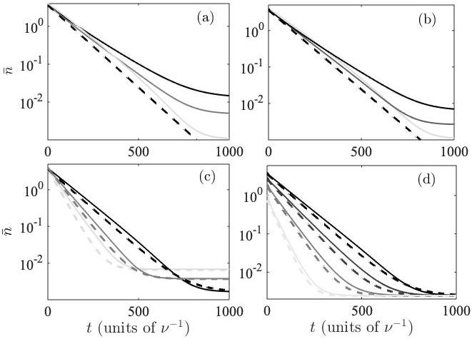
Figure 2: Average phonon occupation $\bar{n}$ for the standing wave sideband cooling as a function of time $t$. In all the panels $\Delta=-\nu$. (a) The black lines from darker to lighter stand for the exact dynamics at $\eta=0.2,0.12,0.04$, while the black dashed line is our analytic prediction. The other parameters used are $n_{0}=4$, $\Omega=1.5\nu$, $\gamma=0.1\nu$. (b) The black lines from darker to lighter stand for the exact dynamics at $\Omega=2.1\nu,1.25\nu,0.6\nu$ respectively, while the black dashed line is our analytic prediction. The other parameters used are $n_{0}=4$, $\eta=0.1$, $\gamma=0.1\nu$. (c) The black lines from darker to lighter stand for the exact dynamics at $\gamma=0.1\nu,0.15\nu,0.2\nu$ respectively with $\Omega=9\gamma$, while the dashed lines from darker to lighter are the corresponding analytic predictions. The other parameters used are $n_{0}=4$, $\eta=0.1$. (d) The black lines from darker to lighter stand for the exact dynamics at $n_{0}=4,3,2,1$ respectively, while the dashed lines from darker to lighter are the corresponding analytic predictions. The other parameters used are $\eta=0.08$, $\Omega=1.5\nu$, $\gamma=0.1\nu$.

To verify our physical picture in the SSC regime, we compare our analytic expression in Eq.(22) with the numerical solutions of the exact Lindblad equation as in Eq.(2). Concretely, We plot the dependence of $\bar{n}$ as a function of time $t$ in Fig. 2 for different values of $\eta$ (panel a), $\Omega$ (panel b), $\gamma$ (panel c) and $n_{0}$ (panel d) respectively. From Fig. 2(a, b) we can see that our analytic expression works better for smaller values of $\eta\Omega/\nu$, which is as expected since Eq.(22) is derived based on the resolved sideband condition. In Fig. 2(c), we have chosen different values of $\gamma$ such that $\eta\Omega/\nu=0.9\gamma/\nu\ll 1$ is satisfied, and we can see that the dynamics predicted by Eq.(22) agrees well with the exact numerical solutions, except that Eq.(22) predicts a slightly faster decay since heating due to the blue sideband is neglected in Eq.(8). In Fig.2(d), we fix $\eta\Omega/\nu=1.2\gamma/\nu=0.12$ and we can see that the cooling rate indeed has a strong dependence on $\bar{n}_{0}$ as predicted by Eq.(21). The numerical simulations throughout this work are done using the open source numerical package QuTiP Johansson et al. (2012).

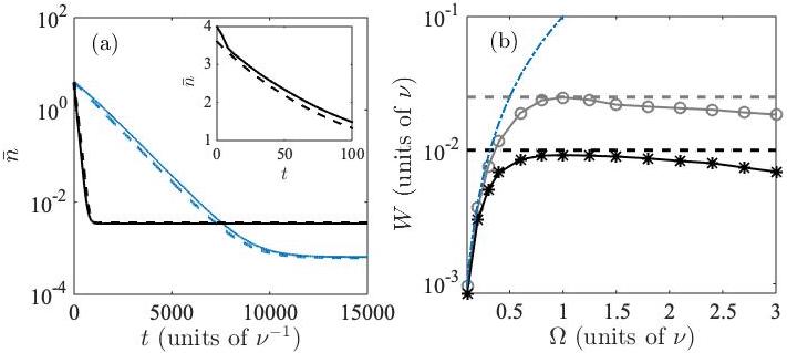
Figure 3: Average phonon occupation $\bar{n}$ as a function of time $t$ for the standing wave sideband cooling. The black line and black dashed line are exact and analytic results in the strong sideband coupling limit with $\Omega=1.5\nu$. The blue line and blue dashed line are exact and analytic results in the weak sideband coupling limit with $\Omega=0.1\nu$. The inset highlights the short time dynamics in the strong sideband coupling limit. We have used $n_{0}=4$ in this panel. (b) The darker black line with star and the darker black dashed line show the exact and analytic cooling rate $W$ as a function of $\Omega$ with $n_{0}=4$, where the exact cooling rate is computed from the exponential fitting of the exact dynamics. The lighter black line with circle and the the lighter black dashed line show the exact and analytic cooling rate $W$ as a function of $\Omega$ with $n_{0}=1$. The blue dot-dashed line is the cooling rate predicted in the weak sideband coupling limit by Eq.(1), which is independent of $n_{0}$. The other parameters used in both panels are $\eta=0.1$, $\Delta=-\nu$, $\gamma=0.1\nu$.

To highlight the sharp differences between the SSC limit and the WSC limit, we compare the dynamics as well as the steady state phonon occupation in both regimes. In Fig. 3(a), we plot $\bar{n}$ as a function of $t$ in the SSC limit (the black line with $\eta\Omega=1.5\gamma$) and in the WSC limit (the blue line with $\eta\Omega=0.1\gamma$), the black and blue dashed lines are the corresponding analytic predictions. In particular, we can see that the cooling rate in the SSC limit is $10$ times larger than in the WSC limit, while the steady state phonon occupation is $5.5$ times larger. In the inset of Fig. 3(a), we plot the short time dynamics in the SSC regime, from which we can see that at the beginning of the cooling dynamics, there is indeed a sudden drop of the average phonon occupation due to the formation of dressed states by rapidly mixing $|g,n\rangle$ with $|e,n-1\rangle$. In Fig. 3(b) we plot the cooling rate, which results from an exponential fitting of the exact dynamics, as a function of the Rabi frequency $\Omega$. The darker black line with star corresponds to $n_{0}=4$ while the lighter black line with circle corresponds to $n_{0}=1$. The darker and lighter black dashed lines are the corresponding analytic predictions from Eq.(18). The blue dot-dashed line is the prediction from Eq.(1). We can see that Eq.(1) agrees well with the numerical fitting when $\Omega/\nu<0.5$, where the WSC condition is satisfied, and then for $1<\Omega/\nu<1.5$, the analytic predictions from Eq.(18) agree well with the numerical fitting. For even larger $\Omega$ such that $\Omega/\nu>2$, the derivation between Eq.(18) and the numerical fitting becomes larger since the resolved sideband condition is no longer satisfied.

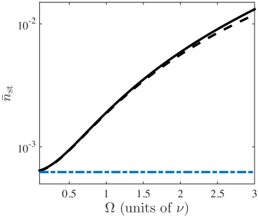
Figure 4: The steady state phonon occupation $\bar{n}_{{\rm st}}$ as a function of the Rabi frequency $\Omega$. The black line and black dashed lines are exact numerical results and our analytic predictions in the strong sideband coupling regime, while the blue dot-dashed represents the analytic results predicted in the weak sideband coupling regime. The other parameters used are $n_{0}=4$, $\eta=0.1$, $\gamma=0.1\nu$, $\Delta=-\nu$.

Finally in Fig. 4, we plot the steady state phonon occupation $\bar{n}_{{\rm st}}$ as a function of $\Omega$. Interestingly, we can see that our analytic prediction in Eq.(21) agrees well with the exact numerical results in all regimes (the derivations which happen for large $\Omega/\nu$ is because that the resolved sideband condition is no longer satisfied.). This is because that to derive Eq.(21) we have kept both the red sideband and the blue sideband terms, and only assumed that the final occupation is close to $0$. The large derivation of $\bar{n}_{\textrm{st},\textrm{WSC}}^{{\rm SW}}$ (the blue dot-dashed line) from the exact result (the black line) again signifies that the $\eta^{2}$ correction term can no longer be neglected when the WSC condition is not satisfied.

III EIT cooling in the SSC limit

Standing wave sideband cooling, being conceptually simple, may have several drawbacks in experimental implementations: 1) The standing wave laser may not be easy to implement and 2) the natural linewidth $\gamma$ is not a tunable parameter and thus the resolved sideband condition $\gamma\ll\nu$ may not be satisfied. The EIT cooling scheme overcomes both difficulties, while at the same time eliminates the carrier transition.

A standard EIT cooling scheme uses a $\Lambda-$type three-level internal structure with an excited state $\left|e\right\rangle$ of linewidth $\gamma$, and two metastable ground states $|g\rangle$ and $|r\rangle$. Two lasers are used, which induce transitions $|g\rangle\leftrightarrow|e\rangle$ and $|r\rangle\leftrightarrow|e\rangle$, with frequencies $\omega_{g}$ and $\omega_{r}$, wave numbers $k_{g}$ and $k_{r}$, Rabi frequencies $\Omega_{g}$ and $\Omega_{r}$ respectively. The internal level structure of EIT cooling is shown in Fig. 5(a). The Hamiltonian of EIT cooling can thus be written as

$$\hat{H}_{{\rm EIT}}= -\Delta|e\rangle\langle e|+\nu\hat{a}^{\dagger}\hat{a}$$

$$+\frac{\Omega_{g}}{2}\left(|g\rangle\langle e|e^{-{\rm i}k_{g}\hat{x}}+|e\rangle\langle g|e^{{\rm i}k_{g}\hat{x}}\right)$$

$$+\frac{\Omega_{r}}{2}\left(|r\rangle\langle e|e^{-{\rm i}k_{r}\hat{x}}+|e\rangle\langle r|e^{{\rm i}k_{r}\hat{x}}\right),$$ (23)

with $\eta_{g}=k_{g}/\sqrt{2m\nu}$ and $\eta_{r}=k_{r}/\sqrt{2m\nu}$, and $\Delta$ being the detuning for both lasers. Similar to Eq.(II), the dissipative part of the EIT cooling can be written as

$$\mathcal{D}_{\textrm{EIT}}(\hat{\rho})$$

$$= \sum_{j=g,r}\gamma_{j}\int_{-1}^{1}d\left(\cos(\theta)\right)\left(\frac{3}{4}\left(1+\cos^{2}(\theta)\right)\right)|j\rangle\langle e|$$

$$e^{{\rm i}k_{j}\hat{x}\cos(\theta)}\hat{\rho}e^{-{\rm i}k_{j}\hat{x}\cos(\theta)}|e\rangle\langle j|-\frac{\gamma_{g}}{2}\{|e\rangle\langle e|,\hat{\rho}\}.$$ (24)

where $\gamma_{g}$ and $\gamma_{r}$ are the decay rates from $|e\rangle$ to $|g\rangle$ and $|r\rangle$ respectively.

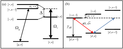
Figure 5: (a) The level diagram of EIT cooling. Two lasers couples $|g\rangle$ and $|r\rangle$ with strengths $\Omega_{g}$ and $\Omega_{r}$ to $|e\rangle$, with the same detuning $\Delta$. The internal Hamiltonian containing the three levels $|g\rangle$, $|r\rangle$ and $|e\rangle$ is diagonalized and results in three dressed state $|d\rangle$, $|+\rangle$ and $|-\rangle$ with energies $\omega_{d}$, $\omega_{+}$, $\omega_{-}$, from lower to higher, as in Eqs.(25, 26). The red sideband resonance condition is satisfied in the dressed state picture by choosing $\omega_{+}=\nu$. (b) After neglecting the far-off resonant coupling from $|d,n\rangle$ to $|-,n\rangle$, the EIT cooling forms a dissipative cascade similar to the standing wave sideband cooling. Strong sideband coupling condition is satisfied if $\eta\Omega\gg\gamma_{{\rm eff}}$.

The internal degrees of freedom of $\hat{H}_{{\rm EIT}}$ can be diagonalized with three eigenstates Fleischhauer et al. (2005)

$$\left|+\right\rangle =\sin\phi\left|e\right\rangle-\cos\phi\left(\sin\vartheta\left|g\right\rangle+\cos\vartheta\left|r\right\rangle\right);$$ (25a)

$$\left|-\right\rangle =\cos\phi\left|e\right\rangle+\sin\phi\left(\sin\vartheta\left|g\right\rangle+\cos\vartheta\left|r\right\rangle\right);$$ (25b)

$$\left|d\right\rangle =\cos\vartheta\left|g\right\rangle-\sin\vartheta\left|r\right\rangle$$ (25c)

with energies

$$\omega_{+} =\frac{1}{2}\left(-\Delta+\sqrt{\Omega_{r}^{2}+\Omega_{g}^{2}+\Delta^{2}}\right);$$ (26a)

$$\omega_{-} =\frac{1}{2}\left(-\Delta-\sqrt{\Omega_{r}^{2}+\Omega_{g}^{2}+\Delta^{2}}\right);$$ (26b)

$$\omega_{d} =0.$$ (26c)

Here, the angles $\phi$ and $\vartheta$ are defined by

$$\tan 2\phi =-\frac{\sqrt{\Omega_{r}^{2}+\Omega_{g}^{2}}}{\Delta};$$ (27)

$$\tan\vartheta =\frac{\Omega_{g}}{\Omega_{r}}.$$ (28)

The EIT cooling condition is chosen as $\omega_{+}=\nu$ such that effective red sideband $\left|d,n\right\rangle\rightarrow\left|+,n-1\right\rangle$ is resonant. In the dressed state basis as defined in Eqs.(25), and neglecting the far-detuned state $\left|-\right\rangle$ as well as the effective blue sideband $|d,n\rangle\leftrightarrow|+,n+1\rangle$, we get an effective Hamiltonian in the interacting picture

$$\hat{H}_{{\rm EIT}}^{{\rm LDR}}=i\eta_{D}\frac{\Omega_{+}}{2}\left(\left|d\right\rangle\left\langle+\right|\hat{a}^{\dagger}-\left|+\right\rangle\left\langle d\right|\hat{a}\right),$$ (29)

with $\eta_{D}=\eta_{g}-\eta_{r}$, and $\Omega_{+}=\frac{\Omega_{g}\Omega_{r}}{\sqrt{\Omega_{r}^{2}+\Omega_{g}^{2}}}\sin\phi$. The effective dissipation in the dressed state basis is

$$\mathcal{D}_{{\rm EIT}}^{{\rm LD}}(\hat{\rho})=\gamma_{\textrm{eff}}\left(\left|d\right\rangle\left\langle+\right|\hat{\rho}\left|+\right\rangle\left\langle d\right|-\frac{1}{2}\{\hat{\rho},\left|+\right\rangle\left\langle+\right|\}\right)$$ (30)

with

$$\gamma_{\textrm{eff}}=\frac{\sin^{2}\phi}{2}\left(\gamma_{g}\cos^{2}\vartheta+\gamma_{r}\sin^{2}\vartheta\right).$$ (31)

Comparing Eqs.(29, 30) with Eqs.(7, 6), we can see that the EIT cooling is equivalent to the standing wave sideband cooling, by making the substitutions $\eta\rightarrow\eta_{D}$, $\Omega\rightarrow\Omega_{+}$ $\gamma\rightarrow\gamma_{{\rm eff}}$, which is shown in Fig. 5(b). As a result, the cooling rate and the steady state phonon occupation for EIT cooling in the SSC regime $\eta_{D}\Omega_{+}\geq\gamma_{\textrm{eff}}$ can be read from Eqs.(18, 21) as

$$W_{\textrm{SSC}}^{{\rm EIT}} =\frac{\gamma_{\textrm{eff}}}{2}\frac{1}{1+n_{0}};$$ (32)

$$\bar{n}_{\textrm{st,SSC}}^{{\rm EIT}} =\frac{1}{8}\left(\frac{\eta_{D}\Omega_{\text{+}}}{\nu}\right)^{2}+\bar{n}_{\textrm{st,WSC}}^{{\rm EIT}}.$$ (33)

with $\bar{n}_{\textrm{st,WSC}}^{{\rm EIT}}=\left(\frac{\gamma}{4\Delta}\right)^{2}$ being steady state average phonon occupation of EIT cooling in WSC regime.

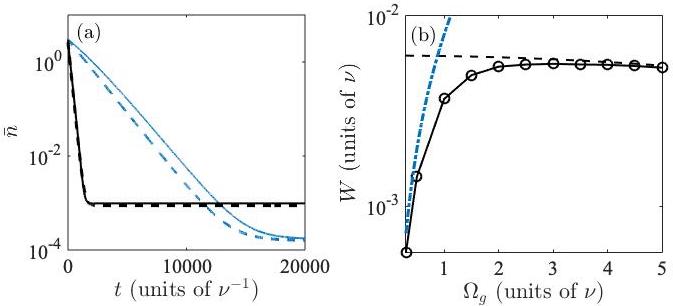
Figure 6: (a) The average photon number $\bar{n}$ as a function of $t$ for EIT cooling. The black and black dashed lines are exact and analytic results in the strong sideband coupling limit with $\Omega_{g}=4\nu$. The blue and blue dashed lines are exact and analytic results in the weak sideband coupling limit with $\Omega_{g}=0.3\nu$. (b) Cooling rate $W$ as a function of the Rabi frequency $\Omega$. The black dashed line represents the analytic predictions from Eq.(34) and the black line with circuit represent the cooling rate from an exponential fitting of the exact dynamics. The blue dashed line is the cooling rate in the weak sideband coupling limit as in Eq.(35). The other parameters used in both panels are $n_{0}=3$, $\eta_{g}=0.1$, $\eta_{r}=-0.1$, $\Delta=103\nu$, $\gamma_{g}=5\nu$, $\gamma_{r}=0$, $\Omega_{r}=20\nu$.

In the experimental implementations of EIT cooling, the coupling strengths are usually chosen such that $\Omega_{g}\ll\Omega_{r}$ Morigi et al. (2000); Roos et al. (2000). As a result the internal dark state $|d\rangle\approx\left|g\right\rangle$. Therefore, we have $\gamma_{\textrm{eff}}\approx\frac{\nu}{\Delta}\gamma_{g}$ and $\Omega_{+}\approx\frac{\Omega_{g}\Omega_{r}}{2\Delta}$, and the cooling rate in SSC regime becomes

$$W_{\textrm{SSC}}^{{\rm EIT}}\approx\frac{\gamma_{g}\nu}{2\Delta}\frac{1}{1+n_{0}}.$$ (34)

Similar to Eq.(18), we can see that the cooling rate is mainly determined by $\gamma_{g}$. In contrast, in the WSC regime, the cooling rate is related to $\gamma=\gamma_{g}+\gamma_{r}$ as

$$W_{\textrm{WSC}}^{{\rm EIT}}\approx\eta_{D}^{2}\frac{\Omega_{g}^{2}}{\gamma},$$ (35)

where in the condition $\Omega_{g}\ll\Omega_{r}$ has been used in deriving the above equation.

Similar to Fig. 3, we compare the sharp difference between EIT cooling in the SSC limit and in the the WSC limit in Fig. 6. In Fig. 6(a), we plot the $\bar{n}$ as a function of time in the SSC limit (the black line with $\eta_{D}\Omega_{+}\approx 3.3\gamma_{{\rm eff}}$) and in the WSC limit (the blue line with $\eta_{D}\Omega_{+}=0.25\gamma_{{\rm eff}}$), the black and blue dashed lines are the corresponding analytic predictions, where we can see that our analytic expressions in Eqs.(32, 33) agree very well with the exact numerical results, and that the cooling rate in the SSC regime is indeed much faster than that in the WSC regime. In Fig. 6(b) we plot the cooling rate resulting from an exponential fitting of the exact dynamics as a function of the Rabi frequency $\Omega_{g}$. We note that in such parameters settings we have $\Omega_{g}\approx\frac{2\Omega_{+}\Delta}{\Omega_{r}}\approx 10\Omega_{+}$ and $\gamma_{{\rm eff}}\approx 0.05\nu$. The black line with circle and the black dashed line correspond to the exact numerical results and the analytic predictions from Eq.(34) respectively, with $n_{0}=3$. The blue dot-dashed line stands for the analytical predictions from Eq.(35). We can see that Eq.(35) agrees well with the exact numerical results when $\Omega_{g}/\nu<0.5$ (corresponding to $\eta_{D}\Omega_{+}/\gamma_{{\rm eff}}<0.2$ where the WSC condition is satisfied). While for $\Omega_{g}/\nu>3$ (corresponding to $\eta_{D}\Omega_{+}/\gamma_{{\rm eff}}>1.2$ where the SSC condition is satisfied), our analytic predictions from Eq.(34) agree well with the exact numerical results.

IV Conclusion

In summary, we have studied standing wave sideband cooling and EIT cooling of trapped ion in the strong sideband coupling regime. We derived analytic expressions for the cooling dynamics as well as for the steady state occupation of the motional state in the strong sideband coupling regime, showing that in this regime we could reach a cooling rate which is proportional to the linewidth $\gamma$ of the excited state , and which also depends on the initial occupation $n_{0}$ of the motional state. This is in comparison with current weak sideband coupling based cooling schemes where the cooling rate is much smaller than $\gamma$ and is independent of $n_{0}$. Additionally, the steady state occupation of the motional state increases by a term proportional to $\eta^{2}$ compared to the weak sideband coupling limit. The analytic expressions are verified against the numerical results by solving the exact Lindblad master equation, showing that they could faithfully recover both the short time and long time dynamics for the motional state of the trapped ion. Our results could be experimentally implemented to speed up the cooling of a trapped ion by a factor of $10$ compared to current weak sideband coupling based schemes such as EIT cooling, and can be easily extended to other dark-state based cooling schemes.

V Acknowledgement

S. Z acknowledges support from National Natural Science Foundation of China under Grant No. 11504430. C. G acknowledges support from National Natural Science Foundation of China under Grant No. 11805279.

References

- Porras and Cirac (2004a) D. Porras and J. I. Cirac, Physical Review Letters 92, 207901 (2004a).
- Porras and Cirac (2004b) D. Porras and J. I. Cirac, Physical Review Letters 93, 263602 (2004b).
- Leibfried et al. (2003) D. Leibfried, R. Blatt, C. Monroe, and D. Wineland, Reviews of Modern Physics 75, 281 (2003).
- Bermúdez et al. (2013) A. Bermúdez, M. Bruderer, and M. B. Plenio, Physical Review Letters 111, 040601 (2013).
- Ruiz et al. (2014) A. Ruiz, D. Alonso, M. B. Plenio, and A. del Campo, Physical Review B 89, 214305 (2014).
- Ramm et al. (2014) M. Ramm, T. Pruttivarasin, and H. Häffner, New Journal of Physics 16, 063062 (2014).
- Guo et al. (2015) C. Guo, M. Mukherjee, and D. Poletti, Physical Review A 92, 023637 (2015).
- Guo and Poletti (2016) C. Guo and D. Poletti, Physical Review A 94, 033610 (2016).
- Guo and Poletti (2017a) C. Guo and D. Poletti, Physical Review A 95, 052107 (2017a).
- Guo and Poletti (2017b) C. Guo and D. Poletti, Physical Review B 96, 165409 (2017b).
- Guo and Poletti (2018) C. Guo and D. Poletti, Physical Review A 98, 052126 (2018).
- Lanyon et al. (2011) B. P. Lanyon, C. Hempel, D. Nigg, M. Müller, R. Gerritsma, F. Zähringer, P. Schindler, J. T. Barreiro, M. Rambach, G. Kirchmair, et al., Science 334, 57 (2011).
- Kielpinski et al. (2002) D. Kielpinski, C. Monroe, and D. J. Wineland, Nature 417, 709 (2002).
- Cirac and Zoller (1995) J. I. Cirac and P. Zoller, Physical Review Letters 74, 4091 (1995).
- Wineland et al. (1998) D. J. Wineland, C. Monroe, W. M. Itano, D. Leibfried, B. E. King, and D. M. Meekhof, Journal of Research of the National Institute of Standards and Technology 103, 259 (1998).
- Diedrich et al. (1989) F. Diedrich, J. Bergquist, W. M. Itano, and D. Wineland, Physical Review Letters 62, 403 (1989).
- Monroe et al. (1995) C. Monroe, D. Meekhof, B. King, S. R. Jefferts, W. M. Itano, D. J. Wineland, and P. Gould, Physical Review Letters 75, 4011 (1995).
- Roos et al. (1999) C. Roos, T. Zeiger, H. Rohde, H. Nägerl, J. Eschner, D. Leibfried, F. Schmidt-Kaler, and R. Blatt, Physical Review Letters 83, 4713 (1999).
- Cohen-Tannoudji et al. (1998) C. Cohen-Tannoudji, J. Dupont-Roc, and G. Grynberg, Atom-photon interactions: basic processes and applications (1998).
- Cirac et al. (1992) J. I. Cirac, R. Blatt, P. Zoller, and W. D. Phillips, Physical Review A 46, 2668 (1992).
- Morigi et al. (2000) G. Morigi, J. Eschner, and C. H. Keitel, Physical Review Letters 85, 4458 (2000).
- Morigi (2003) G. Morigi, Physical Review A 67, 033402 (2003).
- Retzker and Plenio (2007) A. Retzker and M. Plenio, New Journal of Physics 9, 279 (2007).
- Evers and Keitel (2004) J. Evers and C. H. Keitel, EPL (Europhysics Letters) 68, 370 (2004).
- Cerrillo et al. (2010) J. Cerrillo, A. Retzker, and M. B. Plenio, Physical Review Letters 104, 043003 (2010).
- Cerrillo et al. (2018) J. Cerrillo, A. Retzker, and M. B. Plenio, Physical Review A 98, 013423 (2018).
- Albrecht et al. (2011) A. Albrecht, A. Retzker, C. Wunderlich, and M. B. Plenio, New Journal of Physics 13, 033009 (2011).
- Zhang et al. (2012) S. Zhang, C.-W. Wu, and P.-X. Chen, Physical Review A 85, 053420 (2012).
- Zhang et al. (2014) S. Zhang, Q.-H. Duan, C. Guo, C.-W. Wu, W. Wu, and P.-X. Chen, Physical Review A 89, 013402 (2014).
- Lu et al. (2015) Y. Lu, J.-Q. Zhang, J.-M. Cui, D.-Y. Cao, S. Zhang, Y.-F. Huang, C.-F. Li, and G.-C. Guo, Physical Review A 92, 023420 (2015).
- Roos et al. (2000) C. Roos, D. Leibfried, A. Mundt, F. Schmidt-Kaler, J. Eschner, and R. Blatt, Physical Review Letters 85, 5547 (2000).
- Lin et al. (2013) Y. Lin, J. P. Gaebler, T. R. Tan, R. Bowler, J. D. Jost, D. Leibfried, and D. J. Wineland, Physical Review Letters 110, 153002 (2013).
- Kampschulte et al. (2014) T. Kampschulte, W. Alt, S. Manz, M. Martinez-Dorantes, R. Reimann, S. Yoon, D. Meschede, M. Bienert, and G. Morigi, Physical Review A 89, 033404 (2014).
- Lechner et al. (2016) R. Lechner, C. Maier, C. Hempel, P. Jurcevic, B. P. Lanyon, T. Monz, M. Brownnutt, R. Blatt, and C. F. Roos, Physical Review A 93, 053401 (2016).
- Scharnhorst et al. (2018) N. Scharnhorst, J. Cerrillo, J. Kramer, I. D. Leroux, J. B. Wübbena, A. Retzker, and P. O. Schmidt, Physical Review A 98, 023424 (2018).
- Jordan et al. (2019) E. Jordan, K. A. Gilmore, A. Shankar, A. Safavi-Naini, J. G. Bohnet, M. J. Holland, and J. J. Bollinger, Physical Review Letters 122, 053603 (2019).
- Feng et al. (2020) L. Feng, W. Tan, A. De, A. Menon, A. Chu, G. Pagano, and C. Monroe, Physical Review Letters 125, 053001 (2020).
- Qiao et al. (2020) M. Qiao, Y. Wang, Z. Cai, B. Du, P. Wang, C. Luan, W. Chen, H.-R. Noh, and K. Kim, arXiv preprint arXiv:2003.10276 (2020).
- Machnes et al. (2010) S. Machnes, M. B. Plenio, B. Reznik, A. Steane, and A. Retzker, Physical Review Letters 104, 183001 (2010).
- Gorini et al. (1976) V. Gorini, A. Kossakowski, and E. C. G. Sudarshan, J. Math. Phys. 17, 821 (1976).
- Lindblad (1976) G. Lindblad, Comm. Math. Phys. 48, 119 (1976).
- Roos (2000) C. Roos, Controlling the quantum state of trapped ions, Ph.D. thesis (2000).
- Johansson et al. (2012) J. R. Johansson, P. D. Nation, and F. Nori, Computer Physics Communications 183, 1760 (2012).
- Fleischhauer et al. (2005) M. Fleischhauer, A. Imamoglu, and J. P. Marangos, Reviews of Modern Physics 77, 633 (2005).