StressNet: Detecting Stress in Thermal Videos

Abstract

Precise measurement of physiological signals is critical for the effective monitoring of human vital signs. Recent developments in computer vision have demonstrated that signals such as pulse rate and respiration rate can be extracted from digital video of humans, increasing the possibility of contact-less monitoring. This paper presents a novel approach to obtaining physiological signals and classifying stress states from thermal video. The proposed network–”StressNet”–features a hybrid emission representation model that models the direct emission and absorption of heat by the skin and underlying blood vessels. This results in an information-rich feature representation of the face, which is used by spatio-temporal network for reconstructing the ISTI ( Initial Systolic Time Interval : a measure of change in cardiac sympathetic activity that is considered to be a quantitative index of stress in humans). The reconstructed ISTI signal is fed into a stress-detection model to detect and classify the individual’s stress state (i.e. stress or no stress). A detailed evaluation demonstrates that StressNet achieves estimated the ISTI signal with 95% accuracy and detect stress with average precision of 0.842. The source code is available on Github

Keywords:

Stress Detection, rPPG, ISTI signal, physiological signal measurement, ECG, ICG, Deep learning model

1 Introduction

As the world has come to a standstill due to a deadly pandemic [33], the need for non-contact, non-invasive health monitoring systems has become imperative. Remote photoplethysmography (rPPG) provides a way to measure physiological signals remotely without attaching sensors, requiring only video recorded with a high-resolution camera to measure the physiological signals of human health. Much of the recent research in the area of rPPG [50] has focussed on leveraging modern computer vision based systems  [8, 54, 25, 5] to monitor human vitals such as heart rate and breathing rate. More recent work has expanded these methods to detecting more complex human physiological signals and using them to classify stress states  [54, 25, 5].

Figure 1: Example of ECG and $\partial Z/\partial t$ waveforms computed from the present data. $\partial Z/\partial t$ represents the change in impedance recorded by ICG (Z) signal with time. After each ECG peak value there exists an $\partial Z/\partial t$ peak value. The time difference between these two values is known as the initial systolic time interval (ISTI).

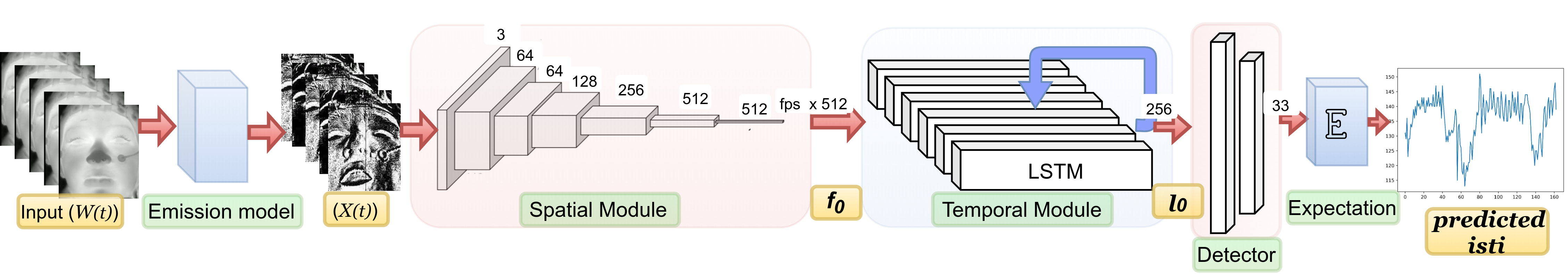
Figure 2: Model Architecture. Green boxes are the different modules of the model. Yellow boxes are the variables throughout the model. The Emission model processes the raw input data which is then fed into spatial and temporal modules. The Detector network predicts ISTI value for each of the frames from the output of these modules. This ISTI signal is used as input in our stress detection network.

Whereas all recent datasets for rPPG only collect electrocardiogram (ECG) as the cardiovascular ground truth signal, here we recorded both ECG and impedance cardiography (ICG). ICG is a noninvasive technology measuring total electrical conductivity of the thorax. It is the measure of change in impedance due to blood flow. With these two signals, we have the ability to estimate more accurate quantifiers of cardiac sympathetic activity [38]. Two common metrics are pre-ejection time (PEP) and initial systolic time interval (ISTI).

PEP is the strongest cue for cardiac sympathetic activity. It is defined as the interval from the onset of left ventricular depolarization, reflected by the Q-wave onset in the ECG, to the opening of the aortic valve, reflected by the B-point in the $\partial Z/\partial t$ (derivative of ICG or Z) signal [32, 52] as can be seen in Figure 1. Unfortunately, measuring PEP from ECG and $\partial Z/\partial t$ signals is quite difficult as the Q and B points that define PEP are subtle and very difficult to pinpoint [37, 46]. Accuracy of methods to estimate PEP are low and precision differs highly among studies [24, 37]. Instead, ISTI can be used as a reliable index of cardiac sympathetic activity [38]. ISTI is a straightforward calculation defined as the time difference between the consecutive peaks of ECG and $\partial Z/\partial t$. ISTI is considered a strong index of myocardial contractility  [46, 26] and numerous efforts have shown that ISTI can be used to analyze different physiological phenomena e.g. stress, blood pressure [26, 51, 47, 26].

Here we introduce StressNet, a non-contact based approach to estimating ISTI. To the best of our knowledge this approach is the first of it’s kind. StressNet leverages the ISTI signal to classify whether a person is experiencing stress or not. To estimate the ISTI signal, a spatial-temporal deep neural network has been developed along with an emission representation model. Other physiological signals like heart rate (HR) or heart rate variability (HRV) cannot measure the changes in contractility, which are influenced by sympathetic, but not by parasympathetic activity, in humans [28].

Recently a number of studies have applied deep learning methods to the detection of HR or HRV from face videos  [54, 8, 19, 29]. Most of these methods either fail to correctly identify the peak information in ECG or do not properly exploit the temporal relations in the face videos  [54]. Recent work by  [54] has developed a spatial-temporal deep network to measure rPPG signals such as heart rate variability (HRV) and average heart rate (AHR). Although these measurements are important, we show that in our experimental setup, the ground-truth ISTI signals allow for more accurate classification of stress state than AHR or HRV.

In addition, thermal images mitigate some privacy concerns because the true likeness of the face is not being stored unlike RGB based models [15].

StressNet is an end-to-end spatial-temporal network that estimates ISTI signal and attempts to classify stress states based on thermal video recordings of the human face. An extensive analysis of the detailed dataset developed for this work has shown correlation between the estimated signal and ground truth. The effectiveness of this predicted ISTI signal is further validated by the model’s ability to accurately classify an individual’s stress state.

Technical Contributions:

• An emission representation module is proposed that can be applied to infrared videos to model variations in emitted radiation due to motion of blood and head movements.

• A spatial temporal deep neural network is developed to estimate ISTI.

• A simple classifier is then trained to estimate the stress level from the computed ISTI signal. To the best of our knowledge this is the first attempt to directly estimate ISTI and stress from thermal video.

2 Related Works

ISTI has been proposed as an effective, quantitative measure of psychological and physiological stress  [21, 31, 12, 18, 6]. Measurement of ISTI requires both the ECG and $\partial Z/\partial t$ signals. Heart rate variability has also been used in several studies to index psychological and physiological stress [54, 8, 19, 29]. Different camera modalities have also been used, namely, infrared, visible RGB, and five-channel multi-spectral [3, 8, 54, 5, 53]. A distinction is also made between research that takes place under laboratory and real-world settings. In the latter, environmental variables can complicate the detection and/or estimation task.

While no other works have included ISTI estimation or the ICG signal in their frameworks, the common video and ECG inputs lend themselves to similar network designs.

Several works for estimation of heart rate rely solely upon registration and classical signal processing techniques. For example, work from [23] registered a region of interest on the face, took the mean of the green channel, and passed that signal through a bandpass filter to estimate the heartbeat signal. At its time of publication in 2014, it achieved state-of-the-art performance on the MAHNOB-HCI dataset with a mean-squared error of 7.62 bpm [23].

Several studies have investigated heart rate variability estimation, using a variety of sensor types [25, 5, 27, 4].

The first end-to-end trainable neural network for rPPG was DeepPhys [8]. It replaced the classical face detection methods with a deep learning attention mechanism. Temporal frame differences are fed to the model, in addition to the current frame, to allow the network to learn motion compensation.

A more recent model built on DeepPhys is PhysNet [54]. This work incorporated a recurrent neural network (RNN), specifically long short term memory (LSTM) over the temporal domain. For tasks such as heart rate detection and pulse detection, modest gains were observed over DeepPhys. The addition of the LSTM also allowed the network to be trained on the task of atrial fibrillation detection.

3 Approach

Using raw thermal videos, our emission representation model generates the input for the spatial-temporal network. This network, along with the detection network predicts the ISTI signal from the raw input thermal videos. Our proposed model architecture is shown in Figure  2.

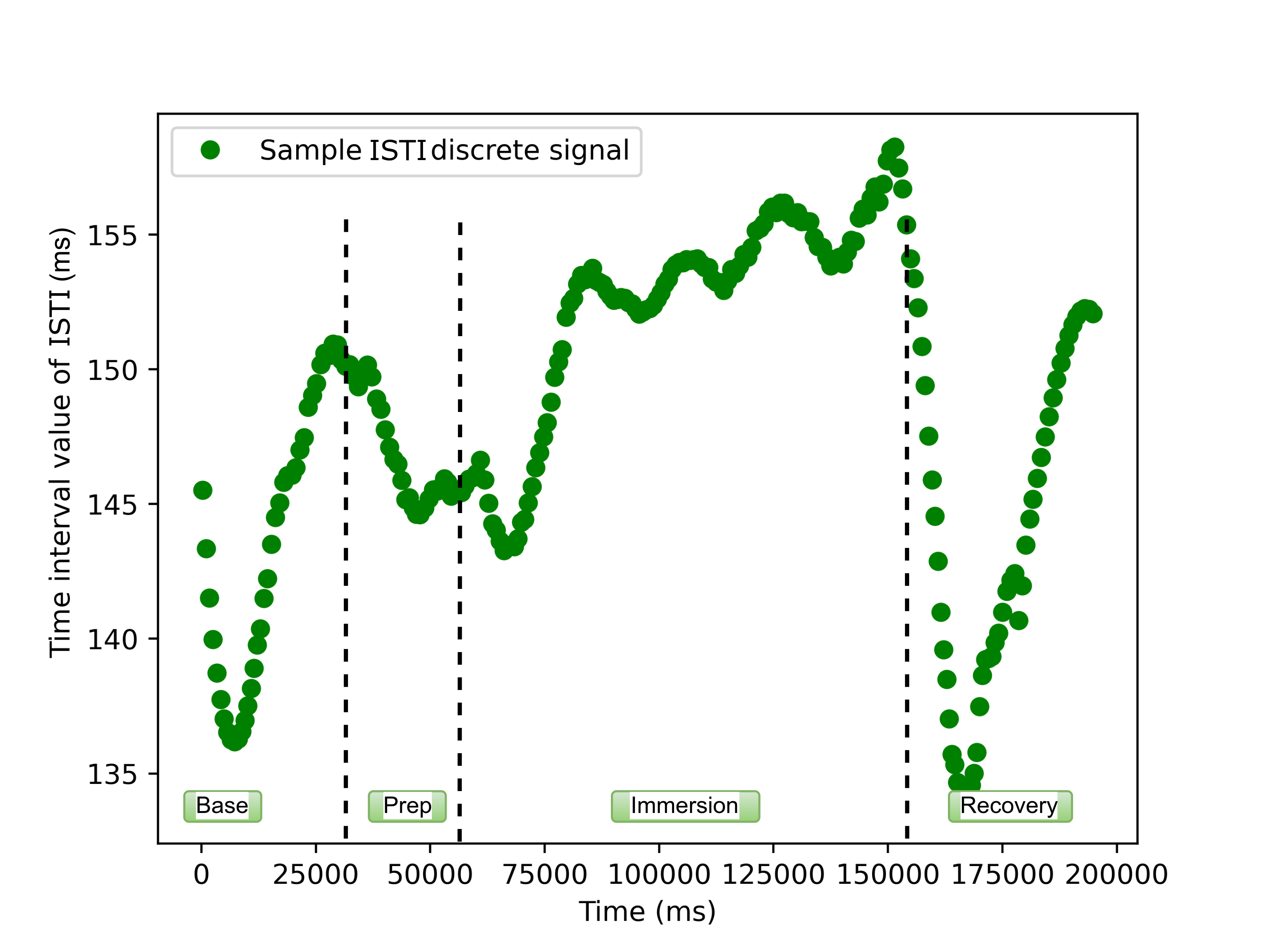
Figure 3: Discrete ISTI values are plotted against the peak positions of the ECG signal for a single participant. The ”Base”, ”Prep”, ”Immersion” and ”Recovery” labels refer to different phases of our stress induction protocol, whereby participants immerse their feet in either ice-water (”stress” condition) or lukewarm water (”no-stress” condition). The data shown were randomly selected from the ”no-stress” condition. See section  4.1 for a detailed description of the protocol.

3.1 Generating ISTI signal

Electrocardiography (ECG) and Impedance cardiography’s (ICG or Z) derivative ($\partial Z/\partial t$) act as the gold-standard physiological signals. ISTI is defined as the interval from the onset of left ventricular depolarization, reflected by the Q-wave onset in the ECG, to the peak blood flow volume through aortic valve, reflected by the Z-point in the $\partial Z/\partial t$ signal. This time interval is computed from each peak of ECG and corresponding $\partial Z/\partial t$ peak. The discrete time interval value of ISTI is plotted at corresponding ECG peak positions as shown in Figure 3 and then interpolated with cubic interpolation to form a continuous signal. In Figure 3, the x-axis represents time (ms) while y-axis values represent the ISTI value (ms) for a particular ECG peak at that time of the video. The interpolated continuous ISTI signal is used as the ground truth for ISTI prediction.

3.2 Emission Representation Model

According to [50], RGB video based physiological signal measurement involves modeling the reflection of external light by skin tissue and blood vessels underneath. However, in the case of thermal videos, the radiation received by the camera involves direct emissions from skin tissue and blood vessels, absorption of radiation from surrounding objects, and absorption of radiation by atmosphere [35, 1]. Here, we build our learning model based on Shafer’s dichromatic reflection model (DRM) [50] as it provides a basic idea to structure our problem of modeling emissions and absorption. We can define the radiation received by the camera at each pixel location $(x,y)$ in the image as a function of time:

$$\textit{{W}}^{x,y}(t)=E_{ems}^{x,y}(t)+E_{abs}^{x,y}(t)+E_{atm}^{x,y}(t)$$ (1)

where $\textit{{W}}(t)$ is an energy vector (we drop the $(x,y)$ pixel location index in the following for simplicity.) $E_{ems}(t)$ is the total emissions from skin tissue and blood vessels; $E_{abs}(t)$ is absorption of radiations by skin tissue and blood vessels; $E_{atm}(t)$ is the absorption of radiation by atmosphere. In current experimental setup the person is in a closed environment and 3ft from thermal camera, therefore the atmospheric absorption is negligible. According to [16], human skin behaves as a black-body radiator, therefore the reflections are close to zero and emission is almost equivalent to absorption.

This implies that the only variation in energy comes from the head motion and from blood flow underneath skin. If we decompose the $E_{ems}(t)$ and $E_{abs}(t)$ into stationary and time-dependent components:

$$E_{ems}(t)=E_{o}\>.\>(\epsilon_{s}+\epsilon_{b}\>.\>f_{1}(m(t),\>p(t))$$ (2)

where $E_{o}$ is the energy emitted by a black body at constant temperature, it is modulated by two components: $\epsilon_{s}$, is the emissivity of skin and $\epsilon_{b}$, is the emissivity of blood. $f_{1}(m(t),\>p(t))$ represents the variations observed by thermal camera;  [8, 50] $m(t)$ denotes all non-physiological variations like head rotations and facial expressions; $p(t)$ is the blood volume pulse (BVP). In a perfect black body, emissivity is equal to absorbtivity, therefore the absorbed energy is:

$$E_{abs}(t)=E_{ab}(t)\>.\>(\epsilon_{s}+\epsilon_{b}\>.\>p(t))$$ (3)

where $E_{ab}$ is the energy absorbed that changes with surrounding objects and their positions with respect to skin tissue.

$$E_{ab}(t)=E_{o}\>.\>(1+f_{2}(m(t),\>p(t)))$$ (4)

where $f_{2}(m(t),\>p(t))$ represents the variation observed by the skin tissue. After substituting (4), (3), (2) in equation (1) and fusing constants; then neglecting the product of $f_{1}$ and $f_{2}$ as it is generally complex non-linear functions. Neglecting product of varying terms, we get an approximate $\textit{{W}}(t)$ as :

$$\begin{split}\textit{{W}}(t)\approx K+E_{o}\>.\>\epsilon_{b}\>.\>(p(t)+f_{1}(m(t),\>p(t)))\\ +E_{o}\>.\>\epsilon_{s}\>.\>f_{2}(m(t)\>,p(t))\end{split}$$ (5)

where K is 2$E_{o}\>.\>\epsilon_{s}$. We can get rid of this constant by taking first order derivative in the temporal domain.

$$\begin{split}\textit{{W}}^{\prime}(t)=p^{\prime}(t)\>.\>E_{o}\>.\>(\epsilon_{b}+\epsilon_{b}\>.\>\frac{\partial f_{1}}{\partial p}+\epsilon_{s}\>.\>\frac{\partial f_{2}}{\partial p})\\ +m^{\prime}(t)\>.\>E_{o}\>.\>(\epsilon_{b}\>.\>\frac{\partial f_{1}}{\partial m}+\epsilon_{s}\>.\>\frac{\partial f_{2}}{\partial m})\end{split}$$ (6)

This representation encompasses all the factors contributing to variations in radiation due to blood and face motion captured by the camera. Thus, we can suppress all possible non-necessary elements from data recorded by the camera. We use $\log$ non-linearity on each pixel to suppress any outlier in each image and separate the $E_{o}$, as its spatial distribution does not contribute to the physiological signal. The non-linearity looks as follows.

$$\textit{{X}}(t)=sign(\textit{{W}}^{\prime}(t))\>.\>\log(1+\mod\textit{{W}}^{\prime}(t))$$ (7)

To remove high frequency components, we do a Gaussian filtering with $\sigma=3$ in the spatial domains, and $\sigma=4$ in the temporal domain. This filtered $\textit{{X}}(t)$ is the input to our deep learning model.

3.3 Deep Learning Model

Spatial-Temporal Network: Spatial-Temporal networks are highly successful in action detection and recognition tasks  [45, 44, 49]. More recently, such networks have been used to process multispectral signals [55, 43, 22] The input to our spatial-temporal network is the stacked features from the emission representation model, which are then fed to a backbone network (e.g. resnet-50 [17]). This backbone network serves as a feature extractor. We mainly tested with object detection networks without the classification blocks as backbone networks.

Weights of these backbone networks are initialized with ImageNet pretrained values so that they can converge quickly on thermal videos. Global average pooling operation follows by the backbone block.

Figure 4: Stress detection network. Estimated ISTI signal is directly fed into the classifier network to predict the probability that the subject is under stress.

$$\textbf{f}_{0}=GAP(B\>(\textit{{X}}(t))$$ (8)

where $B(\>.\>)$ stands for the backbone network, $GAP$ is global average pooling operation, $\textit{{X}}(t)$ is from equation[ 7] (all processed frames stacked horizontally) and $\textbf{f}_{o}$ is the output feature vector.

The backbone network is followed by long short term memory (LSTM) [42, 14] network, which captures the temporal contextual connection information from the extracted spatial features. LSTM [36] units include a ’memory cell’ that capture long range temporal context. A set of gates is used to control the flow of information which in turn helps the LSTM network learn temporal relations among the input features. The extracted feature vector from the backbone network is fed to the LSTM network.

$$\textbf{l}_{o}=L_{STM}\>(\textbf{f}_{0})$$ (9)

where $\textbf{l}_{o}$ is the feature output from LSTM network, $L_{STM}(\>.\>)$ stands for LSTM network and $f_{0}$ is the extracted feature vector from the backbone network.

Detection Network: Instead of directly predicting the continuous value of the ISTI signal from the output of LSTM network, we have divided the whole range [0,1] of ISTI values in $n$ number of bins following [34]. To obtain the exact value of the ISTI signal ($\widehat{\textbf{ISTI}}$) from each frame the expectation of the probability is taken for over all bins ($\widehat{\textbf{isti}}_{bins}$),

$$\begin{split}\widehat{\textbf{isti}}_{bins}=D\>(\textbf{l}_{o});\>\>\widehat{\textbf{ISTI}}=\operatorname{\mathbb{E}}\>(\widehat{\textbf{isti}}_{bins})\end{split}$$ (10)

where D stands for detection network which consists of fully connected layers, $\widehat{\textbf{isti}}_{bins}$ is the probability of each bin, $\operatorname{\mathbb{E}}$ is the Expected value, $\widehat{\textbf{ISTI}}$ is the predicted ISTI value of each frame. This two stage approach makes our network more robust.

The predicted $\widehat{\textbf{ISTI}}$ signal is fed to stress detection network which consists of fully connected layers, see Figure 4. The output of this network is probability of stress for the subject whose ISTI signal is estimated by our spatial-temporal network.

3.4 Multi Loss Approach

Previous works which predicted heart rate, breathing rate, or blood volume pulse mostly use mean squared error (MSE) loss. Another approach bins the regression output, and modifies the network output layer to be a multi-class classification. This method provides more stability to outliers than MSE, but its accuracy is limited by the number of bins. So for the ISTI signal prediction model, we use the multi loss approach used by [34]. This type of loss is a combination of two components: a binned ISTI classification and an ISTI regression loss.

$$\begin{split}\textbf{L}\>(\Theta)=BCE\>(\widehat{\textbf{isti}}_{bins},\>\textbf{isti}_{bins})\>\>+\\ \alpha\>.\>MSE(\widehat{\textbf{ISTI}},\>\textbf{ISTI})\end{split}$$ (11)

For the stress detection network only binary cross entropy (BCE) is used as loss function.

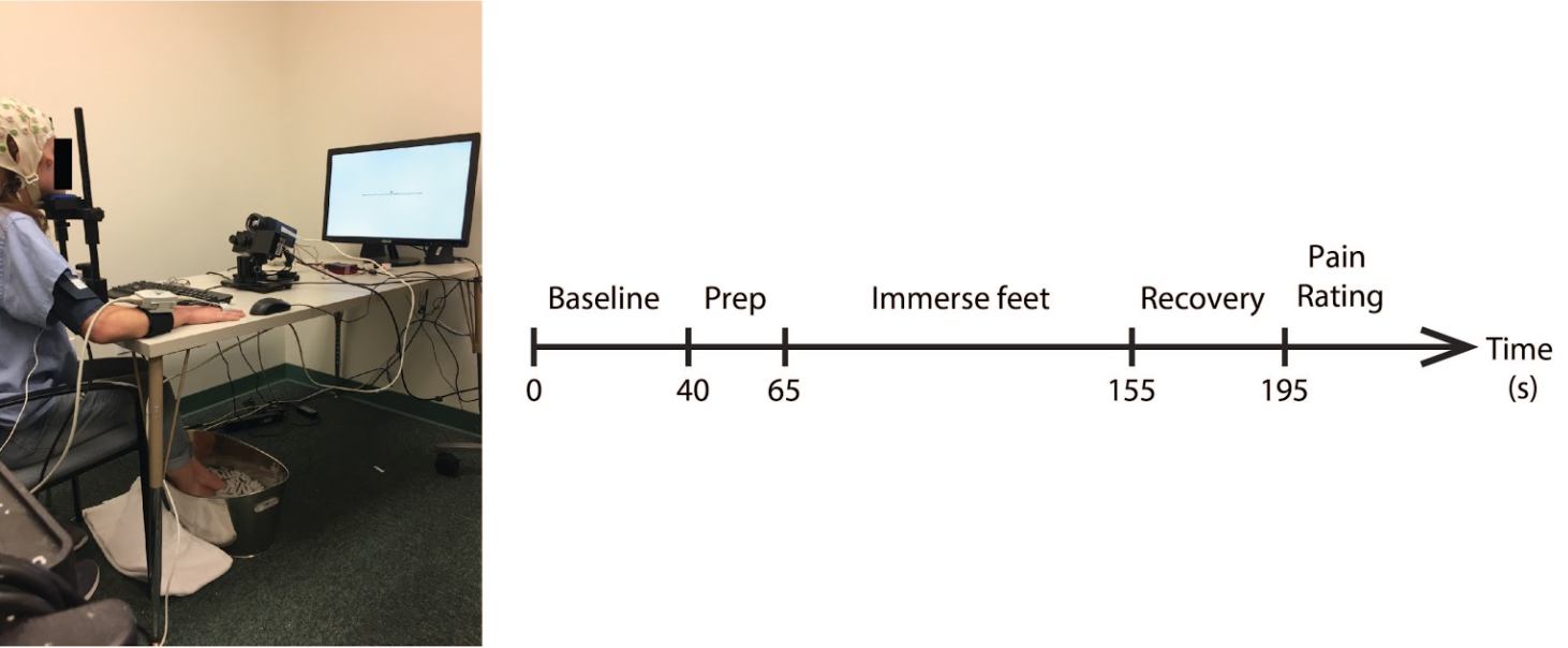
Figure 5: CPT/WPT Setup and Protocol. An example of a fully instrumented participant is shown. Participants followed instructions for the protocol presented on a computer monitor. After the baseline period the participant is instructed to position both feet on the edge of the bucket and prepare for immersion (prep). They then immerse the feet for 90s, then withdraw the feet and rest them on a towel for a 40 s recovery period.

4 Experiments

4.1 Dataset

42 healthy adults (22 males, mean age 20.35 years) were recruited as part of the Biomarkers of Stress States (BOSS) study run at UC Santa Barbara, designed to investigate how different types of stress impact human brain, physiology and behavior. Participants were considered ineligible if any of the following criteria applied: heart condition or joint issues, recent surgeries that would inhibit movement, BMI $>$ 30, currently taking blood pressure medication or any psychostimulants or antidepressants. Informed consent was provided at the beginning of each session, and all procedures were approved by Western IRB and The U.S. Army Human Research Protection Office, and conformed to UC Santa Barbara Human Subjects Committee policies.

Participants attended the lab for five sessions on five separate days as part of the BOSS protocol. For collection of impedance cardiography (ICG), 8 electrodes were placed on the torso and neck, two on each side of the neck and two on each side of the torso. For electrocardiogram (ECG), 2 electrodes were placed on the chest, one under the right collarbone. For videos, thermal camera (Model A655sc, Flir Systems, Wilsonville, OR, USA),was positioned $\sim$65 cm from the participant’s face and set to record at 640 $\times$ 240 pixels and 15 Hz frame rate. A large metal bucket was then positioned in front of the participant’s feet. In the Cold Pressor Test (CPT) session, the bucket was filled with ice water ($\sim$ 0.5 ^∘ C), whereas the in the control session (Warm Pressor Test; WPT), the bucket was filled with lukewarm water ($\sim$ 34 ^∘ C). In each session, participants were required to immerse their feet in the water five times for 90 s, following the test protocol outlined in Figure 5. The CPT is popular method for inducing acute stress in humans in the laboratory. It causes pain and a multiplex of physiological responses e.g. elevated heart rate and blood pressure and increased circulating levels of epinephrine and norepinephrine [56, 2]. The WPT was devised as an ”active” control task, designed such that participants engaged in exactly the same protocol as with the CPT, but without the discomfort of cold-water immersion. This ensured that any psychological or physiological effects induced by engaging in the protocol and immersing the feet in water, were controlled for. Each of the five CPT/WPT immersions were separated by $\sim$ 25 minutes. Between immersions, participants completed tests designed to measure performance across a range of cognitive domains (these data are not reported in this paper). Session order was counterbalanced between participants.

Nine participants’ data were excluded due to technical failures (the thermal imaging camera failed to record one or more sessions). Thirty-three participants’ data were used for modeling. This sample is similar in size to existing public data sets of a similar nature  [40, 20].

4.2 Evaluation Metrics

Performance metrics for evaluating ISTI prediction are Mean Squared Error (MSE) and Pearson’s correlation coefficient (R). For stress detection, average precision (AP) is used as the validation metric.

Mean Squared Error is a model evaluation metric used for regression tasks. The main reason for using MSE as evaluation metric is that the precise value of predicted ISTI signal is important.

Pearson Correlation coefficients are used in statistics to measure how strong a relationship is between two signals. It is defined as covariance of the two signals divided by the product of their standard deviations. Pearson correlation is also used here as an extra validator on the predicted ISTI signal, signifying that the shape of predicted curve also corresponds well with the ground-truth.

$$\rho_{X,Y}=\frac{cov(\>X,\>Y)}{\sigma_{X}\>.\>\sigma_{Y}}$$

Average Precision (AP) is the most commonly used evaluation metric for object detection tasks [10]. It estimates the area under the curve of precision and recall plot. Precision measures how many predictions are correct. Recall calculates the correctly predicted portion of the ground truth values.

4.3 Implementation Details

In experiments, the effectiveness of the spatio-temporal network is evaluated. The dataset is split as follows: 80% training, 10% validation and 10% testing set. The input video frames are cropped to 360 $\times$ 240 to remove the lateral blank areas before being fed to our emission representation model.

For backbone model, experiments with different architectures of resnet were performed, those are resnet18, resnet34, resnet50, resnet101. In the final model resnet50 is used as feature extractor. The output of resnet50 is average-pooled instead of max-pooling operation. The reason for that is removing a less important feature from important feature (max-pool operation) can reduce the signal-to-noise ratio in physiological measurement, so average pooling is used to keep even the less important feature vector information. Before feeding to temporal network, the average-pooled feature vector is reshaped so that each input sequence to LSTM consists of 1 second of time information. The reasoning was that since the peaks of ECG and $\partial Z/\partial t$ signal occurs almost once per second, the LSTM network will better captures the relation between adjacent peaks. For the temporal network, we experimented with a number of LSTM layers (2-8), 6 LSTM layers are best suited for capturing the temporal contextual information. Hidden unit size is kept at half the feature vector length from the spatial network (resnet50), $hidden\_unit\_size$ is 256 $\times$ $frame\_rate$, ensuring that the number of memory cells is sufficient enough to transfer information from previous LSTM cell to next. The number of fully connected layers following LSTM is two, with ReLU added as non-linearity. The output of the final fully connected layer is 33 bins output. 33 bins is an empirical value.

The emission representation model works online in the pipeline and is loaded on the same machine on which deep learning model is trained. Each video is approximately of size (frames $\times$ H $\times$ W) 2500 $\times$ 640 $\times$ 240 with 16bit depth information per pixel. Due to memory constraints on the GPU, $batch\_size$ is kept at 500 frames. The learning rate for resnet50 is started at 0.001, for LSTM and FC layers at 0.01, which reduces after every 10 epochs by a factor of 0.1. Stochastic Gradient Descent is used as optimizer for the network.

Name of the Method	PC Coefficient	MSE
Baseline	0.170	103.829
DeepPhys  [8]	0.575	47.530
I3D  [7] + Detection Network	0.84	5.227
StressNet	0.843	5.845

Table 1: StressNet’s performance in predicting ISTI signal. The performance is measured on Pearson-Correlation Coefficient(PC Coefficient) and mean square error. Our model clearly outperforms the existing methods by a good margin.

5 Results

The proposed method is evaluated in two main criteria. First we evaluated the quality of our predicted ISTI signal, then we tested the effectiveness of the predicted ISTI signal in detecting stress.

Figure 6: Quality of our predicted ISTI signal in stress and no-stress conditions. Data shown are examples from a single participant’s data (selected at random). The ”Base”, ”Prep”, ”Immersion” and ”Recovery” labels refer to the different phases of the CPT/WPT procedure.

Predicting ISTI Signal: For the first part, as mentioned in the evaluation metrics section, the model performance is evaluated on Mean Squared Error (MSE) and Pearson Correlation coefficient (PC Coefficient). In Table 1 our model’s performance can be seen compared to the other methods. Our model outperforms the other methods in both of the evaluation metrics with a good margin. As shown in Figure 6, our model agrees well with the ground truth signal in both stress and no-stress cases.

Since no work has been done on detecting the ISTI signal before, to validate our model we have implemented DeepPhys [8]. As can be seen in Table 1 our implementation of DeepPhys model [8] did not perform well in detecting the ISTI signal. This poor performance mostly stems from two main reasons. First, DeepPhys model is designed to predict periodic physiological signals and since ISTI is non-periodic in nature, loss in DeepPhys does not suit this particular task. Second, the skin reflection model in [8] does not expand properly for modeling the infrared radiation. For baseline methods, ECG signal is extracted from the face using simple statistical filtering methods. According to [9, 13, 48] temperature changes in the tip of the nose and forehead can index different stress states, so for our baseline approach we tracked these regions and then band-pass filtered to extract the signal. This signal is quite noisy which contributes to our baseline’s poor performance.

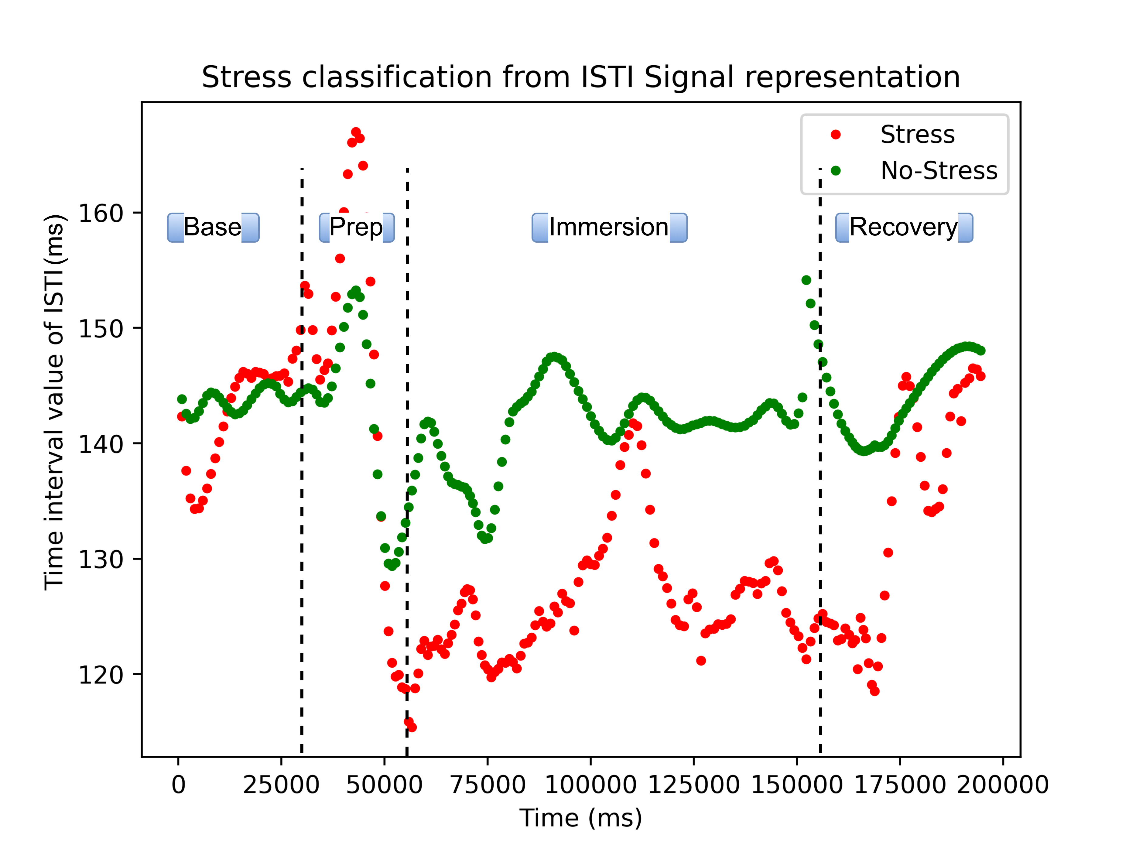
Figure 7: Importance of ISTI signal in detecting stress. Ground truth ISTI data from a single participant (randomly selected) are shown. Clearly, ISTI signal in the stress condition is different from the ISTI signal in no-stress condition. The ”Base”, ”Prep”, ”Immersion” and ”Recovery” labels refer to the different phases of the CPT/WPT procedure.

Input Signal	AP (Average Precision)
Heart Rate (HR)	0.753
Heart Rate Variability(HRV)	0.814
ISTI (Ground Truth Signal)	0.902
ISTI (StressNet Predicted)	0.842

Table 2: StressNet can classify stress state with greater AP using contact-less ISTI estimates when compared to other commonly used contact-less signal estimates (HR and HRV).

Detecting Stress: For the second part of stress detection, we evaluate whether the ISTI signal provides a robust index for stress detection.

An example of the ISTI response to CPT/WPT in a single participant is shown in Figure  7. Here, we observe a clear distinction in ISTI in anticipation of cold- vs. warm- water immersion (i.e. during the prep period) as well as during immersion and recovery.

To evaluate the predictive validity of the ISTI signal, we compare it to heart rate  (HR) and heart rate variability  (HRV) by entering these alternative signals into our model. We compare ISTI with HR and HRV because these measures are considered to be reliable indices of stress [41] and have been used in many stress classification studies [5, 30]. Here, we compute them from the ground truth ECG signal. HR is computed by counting number of beats in a sliding window approach with window size 15 (seconds) and stride 1 (seconds). For HRV, time between R peaks is recorded over a defined time interval (15 seconds) and then HRV is computed according to the Root Mean Square of Successive Differences (RMSSD) method [11].

In Table  2 we can see how our predicted ISTI signal is better in detecting stress state than HR (12% higher AP) and HRV (4 % higher AP). Also, higher AP with the ground truth ISTI signal confirms that ISTI is the most reliable index of stress state in the context of our dataset.

Name of the Backbone	PC Coefficient	MSE
vgg19  [39]	0.605	33.164
resnet18  [17]	0.749	15.095
resnet34  [17]	0.815	6.223
resnet50  [17]	0.843	5.845
resnet101  [17]	0.779	14.373

Table 3: Comparison of different backbones’ performance. In the task of estimating ISTI signal resnet50 is better than all other backbones.

5.1 Ablation Study

Analysis of Emission Representation Model: The overall architecture of StressNet consists of three main models: the emission representation model, the spatial-temporal model and the detection model. To evaluate how each model affects the overall performance, we evaluated the spatial-temporal model with and without the emission representation model. The fully pre-trained network was tested without the emission representation model and we observed a 1.119 increase in the mean squared error in predicting the ISTI signal. The best results for ISTI signal prediction as mentioned in table 1 are obtained using all three models mentioned above.

Analysis with Backbone CNNs: The spatial-temporal model is evaluated with all the ResNet models [17]. We also tested with VGG19 [39] as our backbone. The performance comparison is shown in table 3.

Analysis with Breathing signal: The breathing signal is captured by tracking the area under the nostrils for changes in temperature. The computed time series signal is passed through band-pass filter with low and high cutoff frequencies of 0.1 Hz and 0.85 Hz, respectively. This breathing signal is also used as an input to our stress detection model and the predictions from this model are multiplied with the predicted ISTI signal input. This process boosts the stress detection results by 0.1774 AP. This shows how ISTI can be combined with other physiological signals to detect stress.

Limitations of the Model: Despite being instructed to stay still, participants occasionally made large head movements and/or obscured their face with a hand (see Figure 8). There were also occasions where the ECG/ICG signal was noisy due to movement or bad electrode connections. In these instances the model fails to detect ISTI.

Different Spatial Temporal Network: To validate the effectiveness of spatial temporal networks in detecting ISTI signal, we implemented I3D  [7] architecture, a 3D convolution based spatial-temporal network proposed for action recognition. We replaced the classification branch in I3D with our detection network. The performance is similar to StressNet’s performance.

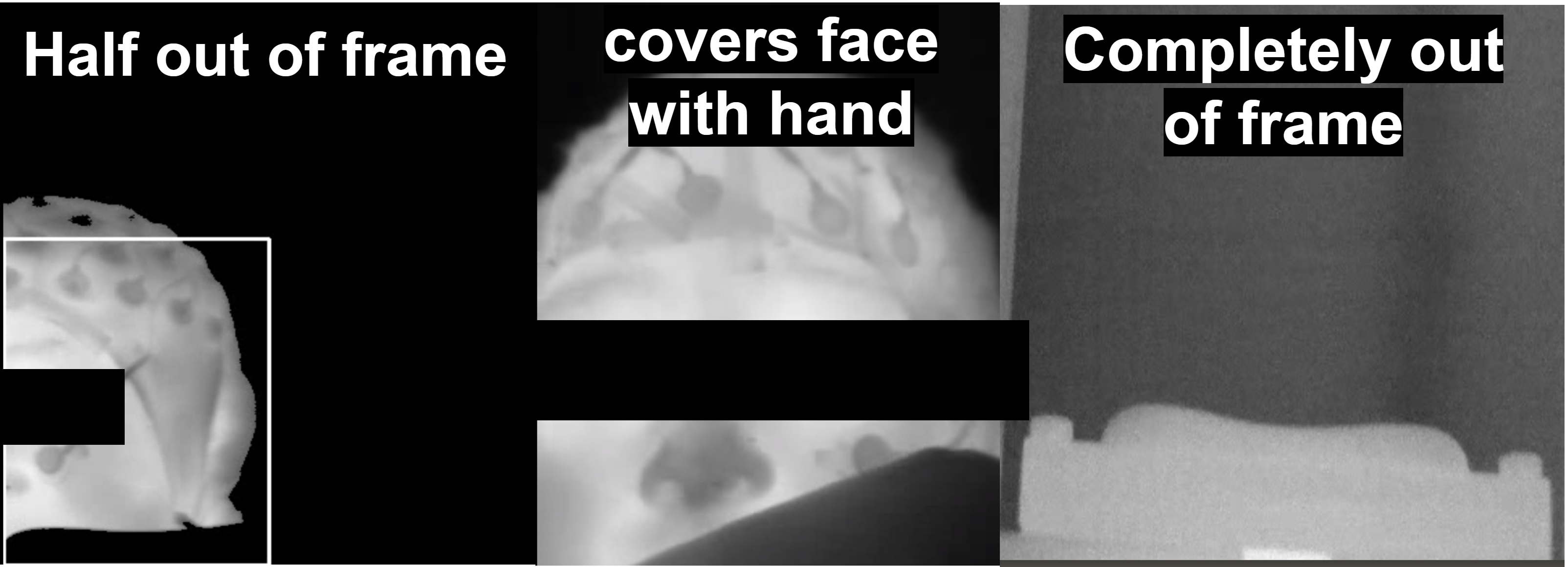
Figure 8: Example StressNet failure cases. Network performance is impaired when the face is outside the video frame or obscured.

6 Conclusion

Here we present a novel method for the estimation of ISTI from thermal video and provide evidence suggesting ISTI is a better index for stress classification than HRV or HR. Overall, our method is more accurate than existing methods when performing binary stress classification on thermal video data.

Our model achieved state-of-the-art performance, and performance could potentially be boosted even further by using different spatial-temporal models. The most successful backbone model used only spatial data from each frame independently, compared to the I3D network [7] that employed simultaneous processing of both spatial and temporal information. However, to test this we require larger dataset, that would allow for improved pre-trained initialization of the spatial-temporal backbones and better transfer learning performance.

This work has several limitations. First, it is unclear whether StressNet’s performance can generalize to the classification of different forms of stress e.g. social stress, physical and mental fatigue. Second, it is possible that exposure to lukewarm-water in the control condition may have induced eustress (beneficial stress), meaning that StressNet is actually classifying distress vs. eustress, not distress vs. neutral states, and this may impact performance. Third, the data used to test StressNet were collected under controlled laboratory conditions, so it is unclear how performance may be impacted in real world use case scenarios that may by subject to increased atmospheric noise and movement artifacts. Further testing with a diverse range of datasets collected under different stress conditions and scenarios is required to determine the efficacy and generalizability of StressNet in the real world.

7 Acknowledgements

This research is supported in part by NSF Award number 1664172 and by the SAGE Junior Fellows Program. The dataset was collected for the UC Santa Barbara Biomarkers of Stress States project, supported by the Institute for Collaborative Biotechnologies through contract W911NF-09-D-0001, and cooperative agreement W911NF-19-2-0026, both from the U.S. Army Research Office.

References

- [1] Kurt Ammer. Temperature effects of thermotherapy determined by infrared measurements. Physica medica, 20:64–66, 2004.
- [2] Petra Bachmann, Xinwei Zhang, Mauro F Larra, Dagmar Rebeck, Karsten Schönbein, Klaus P Koch, and Hartmut Schächinger. Validation of an automated bilateral feet cold pressor test. International Journal of Psychophysiology, 124:62–70, 2018.
- [3] Cristian Paul Bara, Michalis Papakostas, and Rada Mihalcea. A deep learning approach towards multimodal stress detection. In Proceedings of the AAAI-20 Workshop on Affective Content Analysis, New York, USA, AAAI, 2020.
- [4] Timon Blöcher, Johannes Schneider, Markus Schinle, and Wilhelm Stork. An online ppgi approach for camera based heart rate monitoring using beat-to-beat detection. In 2017 IEEE Sensors Applications Symposium (SAS), pages 1–6. IEEE, 2017.
- [5] Frédéric Bousefsaf, Choubeila Maaoui, and Alain Pruski. Remote assessment of the heart rate variability to detect mental stress. In 2013 7th International Conference on Pervasive Computing Technologies for Healthcare and Workshops, pages 348–351. IEEE, 2013.
- [6] Sharon L Brenner and Theodore P Beauchaine. Pre-ejection period reactivity and psychiatric comorbidity prospectively predict substance use initiation among middle-schoolers: A pilot study. Psychophysiology, 48(11):1588–1596, 2011.
- [7] Joao Carreira and Andrew Zisserman. Quo vadis, action recognition? a new model and the kinetics dataset. In proceedings of the IEEE Conference on Computer Vision and Pattern Recognition, pages 6299–6308, 2017.
- [8] Weixuan Chen and Daniel McDuff. Deepphys: Video-based physiological measurement using convolutional attention networks. In Proceedings of the European Conference on Computer Vision (ECCV), pages 349–365, 2018.
- [9] Veronika Engert, Arcangelo Merla, Joshua A Grant, Daniela Cardone, Anita Tusche, and Tania Singer. Exploring the use of thermal infrared imaging in human stress research. PloS one, 9(3):e90782, 2014.
- [10] Mark Everingham, Luc Van Gool, Christopher KI Williams, John Winn, and Andrew Zisserman. The pascal visual object classes (voc) challenge. International journal of computer vision, 88(2):303–338, 2010.
- [11] Bryn Farnsworth. Heart rate variability – how to analyze ecg data. https://imotions.com/blog/heart-rate-variability/, 2019.
- [12] Mohamad Forouzanfar, Fiona C Baker, Ian M Colrain, Aimée Goldstone, and Massimiliano de Zambotti. Automatic analysis of pre-ejection period during sleep using impedance cardiogram. Psychophysiology, 56(7):e13355, 2019.
- [13] Hirokazu Genno, Keiko Ishikawa, Osamu Kanbara, Makoto Kikumoto, Yoshihisa Fujiwara, Ryuuzi Suzuki, and Masato Osumi. Using facial skin temperature to objectively evaluate sensations. International Journal of Industrial Ergonomics, 19(2):161–171, 1997.
- [14] Klaus Greff, Rupesh K Srivastava, Jan Koutník, Bas R Steunebrink, and Jürgen Schmidhuber. Lstm: A search space odyssey. IEEE transactions on neural networks and learning systems, 28(10):2222–2232, 2016.
- [15] Jacob Gunther and Nathan E Ruben. Remote heart rate estimation, Dec. 26 2017. US Patent 9,852,507.
- [16] James D Hardy et al. The radiation of heat from the human body: Iii. the human skin as a black-body radiator. The Journal of clinical investigation, 13(4):615–620, 1934.
- [17] Kaiming He, Xiangyu Zhang, Shaoqing Ren, and Jian Sun. Deep residual learning for image recognition. In Proceedings of the IEEE conference on computer vision and pattern recognition, pages 770–778, 2016.
- [18] J Benjamin Hinnant, Lori Elmore-Staton, and Mona El-Sheikh. Developmental trajectories of respiratory sinus arrhythmia and preejection period in middle childhood. Developmental psychobiology, 53(1):59–68, 2011.
- [19] Gee-Sern Hsu, ArulMurugan Ambikapathi, and Ming-Shiang Chen. Deep learning with time-frequency representation for pulse estimation from facial videos. In 2017 IEEE International Joint Conference on Biometrics (IJCB), pages 383–389. IEEE, 2017.
- [20] Mimansa Jaiswal, Cristian-Paul Bara, Yuanhang Luo, Mihai Burzo, Rada Mihalcea, and Emily Mower Provost. Muse: a multimodal dataset of stressed emotion. In Proceedings of The 12th Language Resources and Evaluation Conference, pages 1499–1510, 2020.
- [21] Robert M Kelsey. Beta-adrenergic cardiovascular reactivity and adaptation to stress: The cardiac pre-ejection period as an index of effort. 2012.
- [22] Satish Kumar, Carlos Torres, Oytun Ulutan, Alana Ayasse, Dar Roberts, and BS Manjunath. Deep remote sensing methods for methane detection in overhead hyperspectral imagery. In The IEEE Winter Conference on Applications of Computer Vision, pages 1776–1785, 2020.
- [23] Xiaobai Li, Jie Chen, Guoying Zhao, and Matti Pietikainen. Remote heart rate measurement from face videos under realistic situations. In Proceedings of the IEEE conference on computer vision and pattern recognition, pages 4264–4271, 2014.
- [24] David L Lozano, Greg Norman, Dayan Knox, Beatrice L Wood, Bruce D Miller, Charles F Emery, and Gary G Berntson. Where to b in dz/dt. Psychophysiology, 44(1):113–119, 2007.
- [25] Daniel McDuff, Sarah Gontarek, and Rosalind Picard. Remote measurement of cognitive stress via heart rate variability. In 2014 36th Annual International Conference of the IEEE Engineering in Medicine and Biology Society, pages 2957–2960. IEEE, 2014.
- [26] Jan H Meijer, Sanne Boesveldt, Eskeline Elbertse, and HW Berendse. Method to measure autonomic control of cardiac function using time interval parameters from impedance cardiography. Physiological measurement, 29(6):S383, 2008.
- [27] Hamed Monkaresi, Nigel Bosch, Rafael A Calvo, and Sidney K D’Mello. Automated detection of engagement using video-based estimation of facial expressions and heart rate. IEEE Transactions on Affective Computing, 8(1):15–28, 2016.
- [28] David B Newlin and Robert W Levenson. Pre-ejection period: Measuring beta-adrenergic influences upon the heart. Psychophysiology, 16(6):546–552, 1979.
- [29] Xuesong Niu, Hu Han, Shiguang Shan, and Xilin Chen. Synrhythm: Learning a deep heart rate estimator from general to specific. In 2018 24th International Conference on Pattern Recognition (ICPR), pages 3580–3585. IEEE, 2018.
- [30] Ulrike Pluntke, Sebastian Gerke, Arvind Sridhar, Jonas Weiss, and Bruno Michel. Evaluation and classification of physical and psychological stress in firefighters using heart rate variability. In 2019 41st Annual International Conference of the IEEE Engineering in Medicine and Biology Society (EMBC), pages 2207–2212. IEEE, 2019.
- [31] K Purushotham Prasad and Dr B Anuradha. Detection of abnormalities in fetal electrocardiogram. International Journal of Applied Engineering Research, 12(1):2017, 2017.
- [32] Harriëtte Riese, Paul FC Groot, Mireille van den Berg, Nina HM Kupper, Ellis HB Magnee, Ellen J Rohaan, Tanja GM Vrijkotte, Gonneke Willemsen, and Eco JC de Geus. Large-scale ensemble averaging of ambulatory impedance cardiograms. Behavior Research Methods, Instruments, & Computers, 35(3):467–477, 2003.
- [33] Max Roser, Hannah Ritchie, Esteban Ortiz-Ospina, and Joe Hasell. Coronavirus pandemic (covid-19). Our World in Data, 2020.
- [34] Nataniel Ruiz, Eunji Chong, and James M Rehg. Fine-grained head pose estimation without keypoints. In Proceedings of the IEEE conference on computer vision and pattern recognition workshops, pages 2074–2083, 2018.
- [35] Francisco J Sanchez-Marin, Sergio Calixto-Carrera, and Carlos Villaseñor-Mora. Novel approach to assess the emissivity of the human skin. Journal of Biomedical Optics, 14(2):024006, 2009.
- [36] Mike Schuster and Kuldip K Paliwal. Bidirectional recurrent neural networks. IEEE transactions on Signal Processing, 45(11):2673–2681, 1997.
- [37] Mark D Seery, Cheryl L Kondrak, Lindsey Streamer, Thomas Saltsman, and Veronica M Lamarche. Preejection period can be calculated using r peak instead of q. Psychophysiology, 53(8):1232–1240, 2016.
- [38] Paul J Silvia. Rz interval as an impedance cardiography measure of effort-related cardiac sympathetic activity paul j. silvia, ashley n. mchone, zuzana mironovová, kari m. eddington, kelly l. harper university of north carolina at greensboro sarah h. sperry, thomas r. kwapil.
- [39] Karen Simonyan and Andrew Zisserman. Very deep convolutional networks for large-scale image recognition. arXiv preprint arXiv:1409.1556, 2014.
- [40] Mohammad Soleymani, Jeroen Lichtenauer, Thierry Pun, and Maja Pantic. A multimodal database for affect recognition and implicit tagging. IEEE transactions on affective computing, 3(1):42–55, 2011.
- [41] Conrad Spellenberg, Peter Heusser, Arndt Büssing, Andreas Savelsbergh, and Dirk Cysarz. Binary symbolic dynamics analysis to detect stress-associated changes of nonstationary heart rate variability. Scientific Reports, 10(1):1–10, 2020.
- [42] Martin Sundermeyer, Ralf Schlüter, and Hermann Ney. Lstm neural networks for language modeling. In Thirteenth annual conference of the international speech communication association, 2012.
- [43] Hanane Teffahi, Hongxun Yao, Souleyman Chaib, and Nasreddine Belabid. A novel spectral-spatial classification technique for multispectral images using extended multi-attribute profiles and sparse autoencoder. Remote Sensing Letters, 10(1):30–38, 2019.
- [44] Oytun Ulutan, ASM Iftekhar, and Bangalore S Manjunath. Vsgnet: Spatial attention network for detecting human object interactions using graph convolutions. In Proceedings of the IEEE/CVF Conference on Computer Vision and Pattern Recognition, pages 13617–13626, 2020.
- [45] Oytun Ulutan, Swati Rallapalli, Mudhakar Srivatsa, Carlos Torres, and BS Manjunath. Actor conditioned attention maps for video action detection. In The IEEE Winter Conference on Applications of Computer Vision, pages 527–536, 2020.
- [46] Maureen AJM Van Eijnatten, Michael J Van Rijssel, Rob JA Peters, Rudolf M Verdaasdonk, and Jan H Meijer. Comparison of cardiac time intervals between echocardiography and impedance cardiography at various heart rates. Journal of electrical bioimpedance, 5(1):2–8, 2014.
- [47] René van Lien, Nienke M Schutte, Jan H Meijer, and Eco JC de Geus. Estimated preejection period (pep) based on the detection of the r-wave and dz/dt-min peaks does not adequately reflect the actual pep across a wide range of laboratory and ambulatory conditions. International Journal of Psychophysiology, 87(1):60–69, 2013.
- [48] H Veltman and W Vos. Facial temperature as a measure of operator state. Foundations of augmented cognition, 293, 2005.
- [49] Limin Wang, Yu Qiao, and Xiaoou Tang. Video action detection with relational dynamic-poselets. In European conference on computer vision, pages 565–580. Springer, 2014.
- [50] Wenjin Wang, Albertus C den Brinker, Sander Stuijk, and Gerard de Haan. Algorithmic principles of remote ppg. IEEE Transactions on Biomedical Engineering, 64(7):1479–1491, 2016.
- [51] Stephen William Wilde, Daniel S Miles, Richard J Durbin, Michael N Sawka, Agaram G Suryaprasad, Robert W Gotshall, and Roger M Glaser. Evaluation of myocardial performance during wheelchair ergometer exercise. American journal of physical medicine, 60(6):277–291, 1981.
- [52] Gonneke HM Willemsen, Eco JC DeGeus, Coert HAM Klaver, Lorenz JP VanDoornen, and Douglas Carrofl. Ambulatory monitoring of the impedance cardiogram. Psychophysiology, 33(2):184–193, 1996.
- [53] Zitong Yu, Xiaobai Li, Xuesong Niu, Jingang Shi, and Guoying Zhao. Autohr: A strong end-to-end baseline for remote heart rate measurement with neural searching. arXiv preprint arXiv:2004.12292, 2020.
- [54] Zitong Yu, Xiaobai Li, and Guoying Zhao. Remote photoplethysmograph signal measurement from facial videos using spatio-temporal networks. In Proc. BMVC, 2019.
- [55] Hui Zhang, Maoguo Gong, Puzhao Zhang, Linzhi Su, and Jiao Shi. Feature-level change detection using deep representation and feature change analysis for multispectral imagery. IEEE Geoscience and Remote Sensing Letters, 13(11):1666–1670, 2016.
- [56] Xinwei Zhang, Petra Bachmann, Thomas M Schilling, Ewald Naumann, Hartmut Schächinger, and Mauro F Larra. Emotional stress regulation: The role of relative frontal alpha asymmetry in shaping the stress response. Biological psychology, 138:231–239, 2018.