Randomized Self Organizing Map

Abstract. We propose a variation of the self organizing map algorithm by considering the random placement of neurons on a two-dimensional manifold, following a blue noise distribution from which various topologies can be derived. These topologies possess random (but controllable) discontinuities that allow for a more flexible self-organization, especially with high-dimensional data. The proposed algorithm is tested on one-, two- and three-dimensions tasks as well as on the MNIST handwritten digits dataset and validated using spectral analysis and topological data analysis tools. We also demonstrate the ability of the randomized self-organizing map to gracefully reorganize itself in case of neural lesion and/or neurogenesis.

1 Introduction

Self-organizing map [25] (SOM) is a vector quantization method that maps data onto a grid, usually two-dimensional and regular. After learning has converged, the codebook is self-organized such that the prototypes associated with two nearby nodes are similar. This is a direct consequence of the underlying topology of the map as well as the learning algorithm that, when presented with a new sample, modifies the code word of the best matching unit (BMU, the unit with the closest to the input code word) as well as the code word of units in its vicinity (neighborhood). SOMs have been used in a vast number of applications [24, 35, 39] and today there exist several variants of the original algorithm [26]. However, according to the survey of [3], only a few of these variants consider an alternative topology for the map, the regular Cartesian and the hexagonal grid being by far the most common used ones. Among the alternatives, the growing neural gas [17] is worth to be mentioned since it relies on a dynamic set of units and builds the topology a posteriori as it is also the case for the incremental grid growing neural network [5] and the controlled growth self organizing map [1]. However, this a posteriori topology is built in the data space as opposed to the neural space. This means that the neighborhood property is lost and two neurons that are close to each other on the map may end with totally different prototypes in the data space. The impact of the network topology on the self-organization has also been studied by [21] using the MNIST database. In the direct problem (evaluating influence of topology on performance), these authors consider SOMs whose neighborhood is defined by a regular, small world or random network and show a weak influence of the topology on the performance of the underlying model. In the inverse problem (searching for the best topology), authors try to optimize the topology of the network using evolutionary algorithms [16] in order to minimize the classification error. Their results indicate a weak correlation between the topology and the performances in this specific case. However, [8] reported contradictory results to [16], when they studied the use of self-organizing map for time series predictions and considered different topologies (spatial, small-world, random and scale-free). They concluded that the classical spatial topology remains the best while the scale-free topology seems inadequate for the time series prediction task. But for the two others (random and small-world), the difference was not so large and topology does not seem to dramatically impact performance.

In this work, we are interested in exploring an alternative topology in order to specifically handle cases where the intrinsic dimension of the data is higher than the dimension of the map. Most of the time, the topology of the SOM is one dimensional (linear network) or two dimensional (regular or hexagonal grid) and this may not correspond to the intrinsic dimension of the data, especially in the high dimensional case. This may result in the non-preservation of the topology [46] with potentially multiple foldings of the map. The problem is even harder considering the data are unknown at the time of construction of the network. To overcome this topological constraint, we propose a variation of the self organizing map algorithm by considering the random placement of neurons on a two-dimensional manifold, following a blue noise distribution from which various topologies can be derived. These topologies possess random discontinuities that allow for a more flexible self-organization, especially with high-dimensional data. After introducing the methods, the model will be illustrated and analyzed using several classical examples and its properties will be more finely introduced. Finally, we’ll explain how this model can be made resilient to neural gain or loss by reorganizing the neural sheet using the centroidal Voronoi tesselation.

A constant issue with self-organizing maps is how can we measure the quality of a map. In SOM’s literature, there is neither one measure to rule them all nor a single general recipe on how to measure the quality of the map. Some of the usual measures are the distortion [42], the $\delta x-\delta y$ representation [11], and many other specialized measures for rectangular grids or specific types of SOMs [38]. However, most of those measures cannot be used in this work since we do not use a standard grid for laying over the neural space, instead we use a randomly distributed graph (see supplementary material for standard measures). This and the fact that the neural space is discrete introduce a significant challenge on deciding what will be a good measure for our comparisons [38] (i.e., to compare the neural spaces of RSOM and regular SOM with the input space). According to [38], the quality of the map’s organization can be considered equivalent to topology preservation. Therefore, a topological tool such as the persistent homology can help in comparing the input space with the neural one. Topological Data Analysis (TDA) is a relatively new field of applied mathematics and offers a great deal of topological and geometrical tools to analyze point cloud data [9, 19]. Such TDA methods have been proposed in [38], however TDA wasn’t that advanced and popular back then. Therefore, in this work we use the persistent homology and barcodes to analyze our results and compare the neural spaces generated by the SOM algorithms with the input spaces. We provide more details about TDA and persistent homology later in the corresponding section.

To avoid confusion between the original SOM proposed by Teuvo Kohonen and the newly randomized SOM, we’ll refer to the original as SOM and the newly randomized one as RSOM.

2 Methods

2.1 Notation

In the following, we will use definitions and notations introduced by [41] where a neural map is defined as the projection from a manifold $\Omega\subset\mathbb{R}^{d}$ onto a set $\mathcal{N}$ of $n$ neurons which is formally written as $\Phi:\Omega\rightarrow\mathcal{N}$. Each neuron $i$ is associated with a code word $\mathbf{w}_{i}\in\mathbb{R}^{d}$, all of which establish the set $\{\mathbf{w}_{i}\}_{i\in\mathcal{N}}$ that is referred as the code book. The mapping from $\Omega$ to $\mathcal{N}$ is a closest-neighbor winner-take-all rule such that any vector $\mathbf{v}\in\Omega$ is mapped to a neuron $i$ with the code $\mathbf{w}_{\mathbf{v}}$ being closest to the actual presented stimulus vector $\mathbf{v}$,

$$\Phi:\mathbf{v}\mapsto argmin_{i\in\mathcal{N}}(\lVert\mathbf{v}-\mathbf{w}_{i}\rVert).$$ (1)

The neuron $\mathbf{w}_{\mathbf{v}}$ is named the best matching unit (BMU) and the set $C_{i}=\{x\in\Omega|\Phi(x)=\mathbf{w}_{i}\}$ defines the receptive field of the neuron $i$.

2.2 Spatial distribution

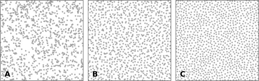
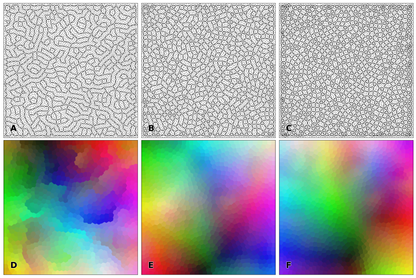
The SOM space is usually defined as a two-dimensional region where nodes are arranged in a regular lattice (rectangular or hexagonal). Here, we consider instead the random placement of neurons with a specific spectral distribution (blue noise). As explained in [47], the spectral distribution property of noise patterns is often described in terms of the Fourier spectrum color. White noise corresponds to a flat spectrum with equal energy distributed in all frequency bands while blue noise has weak low-frequency energy, but strong high-frequency energy. In other words, blue noise has intuitively good properties with points evenly spread without visible structure (see figure 1 for a comparison of spatial distributions).

Figure 1: Spatial distributions. A. Uniform sampling (n=1000) corresponding to white noise. B. Regular grid (n=32$\times$32) + jitter (2.5%). C. Poisson disc sampling (n=988) corresponding to blue noise.

There exists several methods [27] to obtain blue noise sampling that have been originally designed for computer graphics (e.g. Poisson disk sampling, dart throwing, relaxation, tiling, etc.). Among these methods, the fast Poisson disk sampling in arbitrary dimensions [7] is among the fastest ($\mathcal{O}(n)$) and easiest to use. This is the one we retained for the placement of neurons over the normalized region $[0,1]\times[0,1]$. Such Poisson disk sampling guarantees that samples are no closer to each other than a specified minimum radius. This initial placement is further refined by applying a LLoyd relaxation [31] scheme for 10 iterations, achieving a quasi centroidal Voronoi tesselation.

2.3 Topology

Considering a set of $n$ points $P=\{P_{i}\}_{i\in[1,n]}$ on a finite region, we first compute the Euclidean distance matrix $E$, where $e_{ij}=\lVert P_{i}-P_{j}\rVert$ and we subsequently define a connectivity matrix $G^{p}$ such that only the $p$ closest points are connected. More precisely, if $P_{j}$ is among the $p$ closest neighbours of $P_{i}$ then $g^{p}_{ij}=1$ else we have $g^{p}_{ij}=0$. From this connectivity matrix representing a graph, we compute the length of the shortest path between each pair of nodes and stored them into a distance matrix $D^{p}$. Note that lengths are measured in the number of nodes between two nodes such that two nearby points (relatively to the Euclidean distance) may have a corresponding long graph distance as illustrated in figure 2. This matrix distance is then normalized by dividing it by the maximum distance between two nodes such that the maximum distance in the matrix is 1. In the singular case when two nodes cannot be connected through the graph, we recompute a spatial distribution until all nodes can be connected.

Figure 2: Influence of the number of neighbours on the graph distance. The same initial set of 1003 neurons has been equiped with 2-nearest neighbors, 3 nearest neighbors and 4-nearest neighbors induced topology (panels A, B and C respectively). A sample path from the the lower-left neuron to the upper-right neuron has been highlighted with a thick line (with respective lengths of 59, 50 and 46 nodes).

2.4 Learning

The learning process is an iterative process between time $t=0$ and time $t=t_{f}\in\mathbb{N}^{+}$ where vectors $\mathbf{v}\in\Omega$ are sequentially presented to the map. For each presented vector $\mathbf{v}$ at time $t$, a winner $s\in\mathcal{N}$ is determined according to equation (1). All codes $\mathbf{w}_{i}$ from the code book are shifted towards $\mathbf{v}$ according to

$$\Delta\mathbf{w}_{i}=\varepsilon(t)~{}h_{\sigma}(t,i,s)~{}(\mathbf{v}-\mathbf{w}_{i})$$ (2)

with $h_{\sigma}(t,i,j)$ being a neighborhood function of the form

$$h_{\sigma}(t,i,j)=e^{-\frac{{d^{p}_{ij}}^{2}}{\sigma(t)^{2}}}$$ (3)

where $\varepsilon(t)\in\mathbb{R}$ is the learning rate and $\sigma(t)\in\mathbb{R}$ is the width of the neighborhood defined as

$$\sigma(t)=\sigma_{i}\left(\frac{\sigma_{f}}{\sigma_{i}}\right)^{t/t_{f}},\text{ with }\varepsilon(t)=\varepsilon_{i}\left(\frac{\varepsilon_{f}}{\varepsilon_{i}}\right)^{t/t_{f}},$$ (4)

while $\sigma_{i}$ and $\sigma_{f}$ are respectively the initial and final neighborhood width and $\varepsilon_{i}$ and $\varepsilon_{f}$ are respectively the initial and final learning rate. We usually have $\sigma_{f}\ll\sigma_{i}$ and $\varepsilon_{f}\ll\varepsilon_{i}$.

2.5 Analysis Tools

In order to analyze and compare the results of RSOM and SOM, we used a spectral method and persistence diagram analysis on the respective codebooks. These analysis tools are detailed below but roughly, the spectral method allows to estimate the distributions of eigenvalues in the activity of the maps while the persistence diagram allows to check for discrepancies between the topology of the input space and the topology of the map.

Topological Data Analysis (TDA) [9] provides methods and tools to study topological structures of data sets such as point cloud and is useful when geometrical or topological information is not apparent within a data set. Furthermore, TDA tools are insensitive to dimension reduction and noise which make them well suited to analyze high-dimensional self-organized maps and their corresponding input data sets. In this work, we use the notion of persistent barcodes and diagrams [15] to spot any differences between the topology of the input and neural spaces. Furthermore, we can apply some metrics from TDA such as the Bottleneck distance and measure how close two persistent diagrams are. Since the exact manifold (or distribution) of the input space is not known in general and the SOM algorithms only approximate it, we simplify these manifolds by retaining their original topological structure. Here we approach the manifolds of input and neural spaces using the Alpha complex. Before diving into more details regarding TDA, we provide here a few definitions and some notation. A $k$-simplex $\sigma$ is the convex hull of $k+1$ affinely independent points (for instance a $0$-simplex is a point, a $1$-simplex is an edge, a $2$-simplex is a triangle, etc). A simplicial complex with vertex set $\mathcal{V}$ is a set $\mathcal{S}$ of finite subsets of $\mathcal{V}$ such that the elements of $\mathcal{V}$ belong to $\mathcal{S}$ and for any $\sigma\in\mathcal{S}$ any subset $\sigma$ belongs to $\mathcal{S}$. Said differently, a simplicial complex is a space that has been constructed out of intervals, triangles, and other higher dimensional simplices.

In our analysis we let $\mathcal{S}(\mathcal{M},\alpha)$ be a Alpha simplicial complex with $\mathcal{M}$ being a point cloud, either the input space or the neural one, and $\alpha$ is the “persistence” parameter. More specifically, $\alpha$ is a threshold (or radius as we will see later) that determines if the set $X$ spans a $k$-simplex if and only if $d(x_{i},x_{j})\leq\alpha$ for all $0\leq i,j\leq k$. From a practical point of view, we first define a family of thresholds $\alpha$ (or radius) and for each $\alpha$, we center a ball of radius $\alpha$ on each data point and look for possible intersections with other balls. This process is called filtration of simplicial complexes. We start from a small $\alpha$ where there are no intersecting balls (disjoint set of balls) and steadily we increase the size of $\alpha$ up to a point where a single connected blob emerges. As $\alpha$ varies from a low to a large value, holes open and close as different balls start intersecting. Every time an intersection emerges we assign a birth point $b_{i}$ and as the $\alpha$ increases and some new intersections of larger simplicies emerge some of the old simplicies die (since they merge with other smaller simplicies to form larger ones). Then we assign a death point $d_{i}$. A pair of a birth and death points $(b_{i},d_{i})$ is plotted on a Cartesian two-dimensional plane and indicates when a simplicial complex was created and when it died. This two-dimensional diagram is called persistent diagram and the pairs (birth, death) that last longer reflect significant topological properties. The longevity of birth-death pairs is more clear in the persistent barcodes where the lifespan of such a pair is depicted as a straight line.

In other words, for each value of $\alpha$ we obtain new simplicial complexes and thus new topological properties such as homology are revealed. Homology encodes the number of points, holes, or voids in a space. For more thorough reading we refer the reader to [10, 18, 48]. In this work, we used the Gudhi library [32] to compute the Alpha simplicial complexes, the filtrations and the persistent diagrams and barcodes. Therefore, we compute the persistent diagram and persistent barcode of the input space and of the maps and we calculate the Bottleneck distance between the input and SOM and RSOM maps diagrams. The bottleneck distance provides a tool to compare two persistent diagrams in a quantitative way. The Bottleneck distance between two persistent diagrams $\text{dgm}_{1}$ and $\text{dgm}_{2}$ as it is described in [10]

$$d_{b}(\text{dgm}_{1},\text{dgm}_{2}) =\inf_{\text{matching }m}\{\max_{(p,q)\in m}\{||p-q||_{\infty}\}\},$$ (5)

where $p\in\text{dgm}_{1}\backslash\Delta$, $q\in\text{dgm}_{2}\backslash\Delta$, $\Delta$ is the diagonal of the persistent diagram (the diagonal $\Delta$ represents all the points that they die the very moment they get born, $b=d$). A matching between two diagrams $\text{dgm}_{1}$ and $\text{dgm}_{2}$ is a subset $m\subset\text{dgm}_{1}\times\text{dgm}_{2}$ such that every point in $\text{dgm}_{1}\backslash\Delta$ and $\text{dgm}_{2}\backslash\Delta$ appears exactly once in $m$.

2.6 Simulation Details

Unless specified otherwise, all the models were parameterized using values given in table 1. These values were chosen to be simple and do not really impact the performance of the model. All simulations and figures were produced using the Python scientific stack, namely, SciPy [22], Matplotlib [20], NumPy [44], Scikit-Learn [37]. Analysis were performed using Gudhi [32]). Sources are available at github.com/rougier/VSOM.

Parameter	Value
Number of epochs ($t_{f}$)	25000
Learning rate initial ($\varepsilon_{i}$)	0.50
Learning rate final ($\varepsilon_{f}$)	0.01
Sigma initial ($\sigma_{i}$)	0.50
Sigma final ($\sigma_{f}$)	0.01

Table 1: Default parameters Unless specified otherwise, these are the parameters used in all the simulations.

3 Results

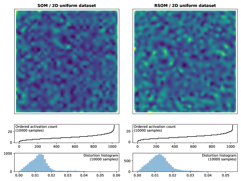
We ran several experiments to better characterize the properties of the randomized SOM and to compare them to the properties of a regular two-dimensional SOM. More specifically, we ran experiments using one dimensional, two dimensional and three dimensional datasets using uniform or shaped distributions. In this section, we only report a two-dimensional case and a three-dimensional case that we consider to be the most illustrative (all other results can be found in the supplementary material). We additionally ran an experiment using the MNIST hand-written data set and we compared it with a regular SOM. Finally, the last experiment is specific to the randomized SOM and shows how the model can recover from the removal (lesion) or the addition (neurogenesis) of neurons while conserving the overall self-organization. Each experiment (but the last) has been ran for both the randomized SOM and the regular SOM even though only the results for the randomized SOM are shown graphically in a dedicated figure while for the analysis, we use results from both SOM and RSOM. The reason to not show regular SOM results is that we assume the behavior is well known and does not need to be further detailed.

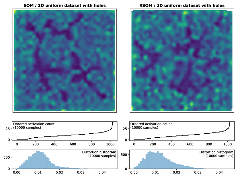
3.1 Two dimensional uniform dataset with holes

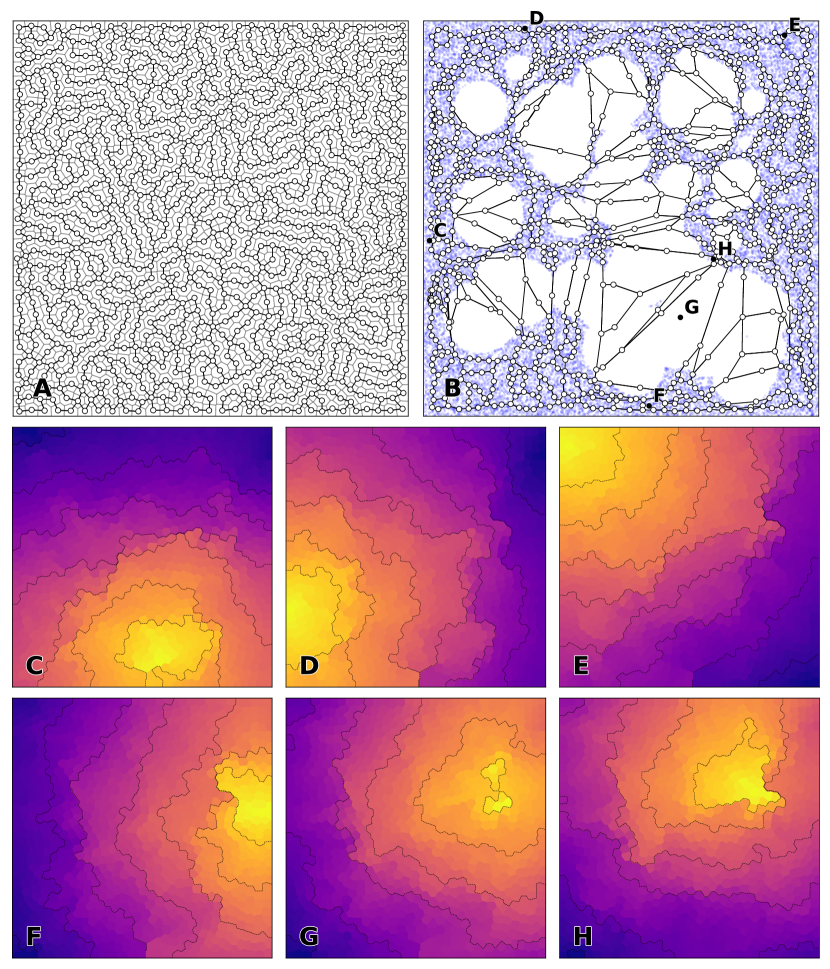
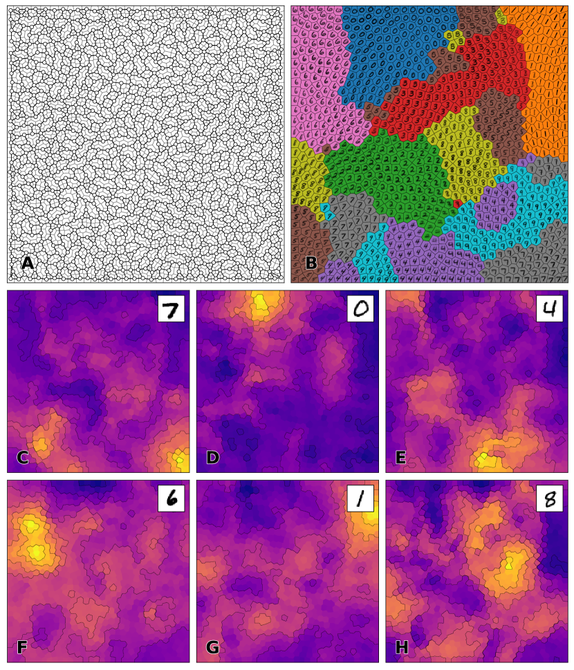
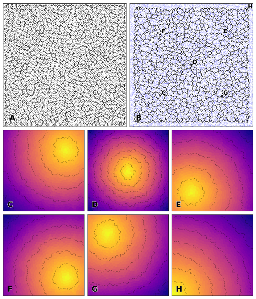
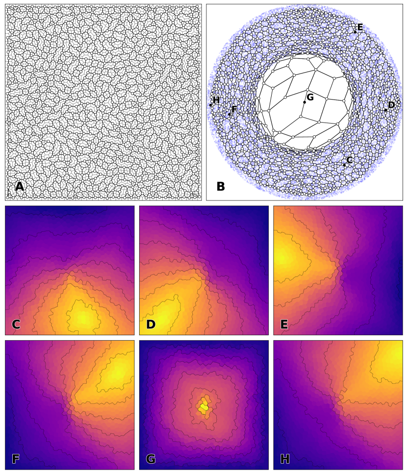
In order to test for the adaptability of the randomized SOM to different topologies, we created a two dimensional uniform dataset with holes of various size and at random positions (see figure 3B). Such holes are known to pose difficulties to the regular SOM since neurons whose codewords are over a hole (or in the immediate vicinity) are attracted by neurons outside the holes from all sides. Those neurons hence become dead units that never win the competition. In the RSOM, this problem exists but is less severe thanks to the absence of regularity in the underlying neural topology and the loose constraints (we use 2 neighbors to build the topology). This can be observed in 3B) where the number of dead units is rather small and some holes are totally devoid of any neurons. Furthermore, when a sample that does not belong to the original distribution is presented, it can be observed that the answer of the map is maximal for a few neurons only (see figure 3G)).

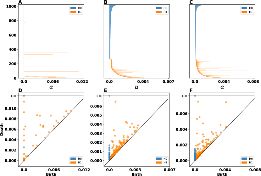
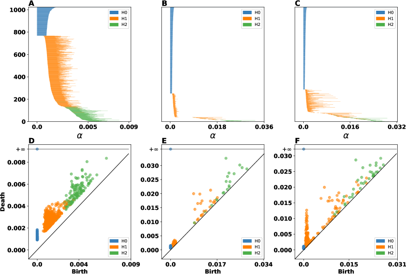
This observation is also supported by our topological analysis shown in figure 4. Figures 4A, B, and C show the persistent barcodes where we can see the lifespan of each (birth, death) pair (for more details about how we compute these diagrams see Section 2.5). We observe that both the SOM and the RSOM capture both the $H0$- and $H1$-homology of the input space, however the RSOM seems to have more persistent topological features for the $H1$-homology (orange lines). This means that the RSOM can capture more accurately the holes which are present in the input space. Roughly speaking we have about eight holes (see figure 3B) and we count about eight persistent features (the longest line segments in the barcode diagrams) for RSOM in 4C. On the other hand, the important persistent features for the SOM are about five. In a similar way the persistent diagrams in figures 4C, D, and E show that both RSOM and SOM capture in a similar way both the $H0$- and $H1$-homology features, although the RSOM (panel F) captures more holes as the isolated orange points away from the diagonal line indicate. This is because the pairs that are further away from the diagonal are the most important meaning that they represent topological features that are the most persistent during the filtration process. Furthermore, we measure the Bottleneck distance between the persistence diagrams of input space and those of SOM and RSOM. The SOM’s persistence diagram for $H0$ is closer to the input space (SOM: $0.000829$, RSOM: $0.001$), while the RSOM’s persistence diagram is closer to input’s one for the $H1$ (SOM: $0.00478$, RSOM: $0.0037$). Finally, we ought to point out that the scale between panels A (D) and B, C (E, F) are not the same since the self-organization process has compressed information during mapping the input space to neural one.

Figure 3: Two dimensional uniform dataset with holes (results) Randomized SOM made of $1024$ neurons with a $2$-nearest neighbors induced topology. Model has been trained for $25,000$ epochs on two-dimensional points drawn from a uniform distribution on the unit square with holes of various sizes and random positions. A Map topology in neural space. B Map topology in data space. C to H Normalized distance map for six random samples. The G point has been purposely set outside the point distribution. Normalization has been performed for each sample in order to enhance contrast but this prevents comparison between maps.

Figure 4: Two dimensional uniform dataset with holes (analysis) Persistent Barcodes of A input space, B SOM, and RSOM. The blue and orange line segments represent the $H0$- and $H1$-homology, respectively. This means that blue color represents connected segments within the space and orange color reflects the holes within the space. The longer the line segment the more important the corresponding topological feature. D illustrates the persistent diagram for the input space. E and F depict the persistent diagrams for SOM and RSOM, respectively. Again blue dots indicate $H0$-homology features and orange dots represent $H1$-homological features.

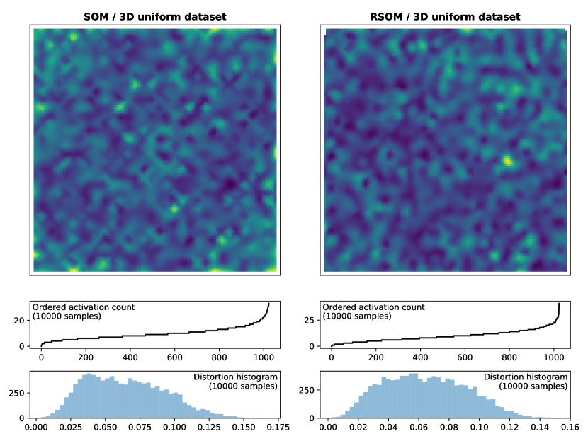
3.2 Three dimensional uniform dataset

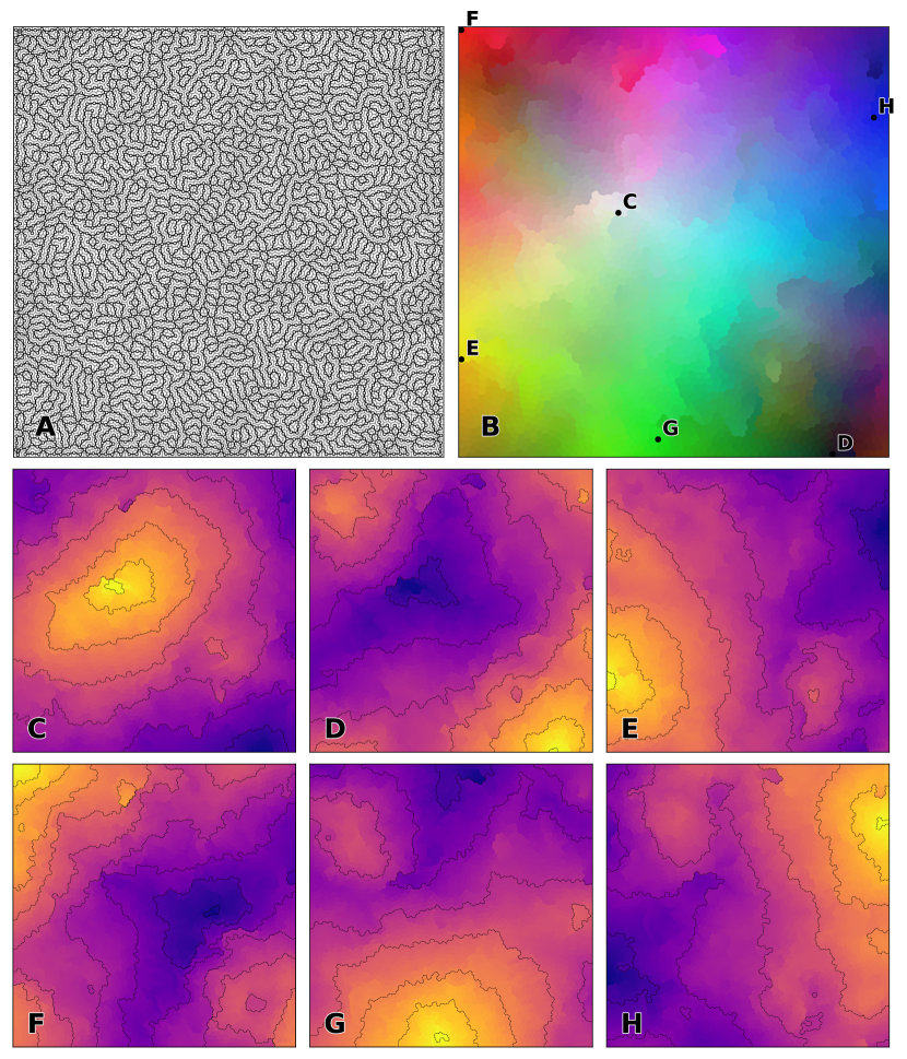
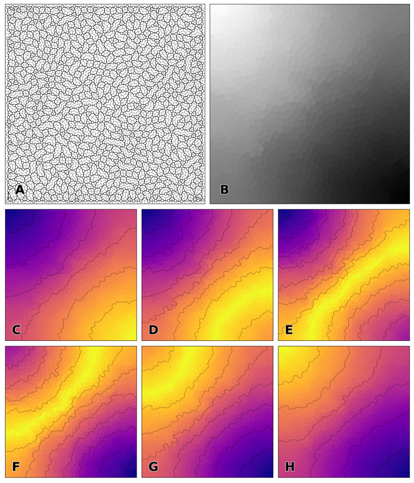
The three dimensional uniform dataset (that corresponds to the RGB color cube) is an interesting low dimensional case that requires a dimensionality reduction (from dimension 3 to 2). Since we used a uniform distribution this means the dataset is a dense three dimensional manifold that needs to be mapped to a two dimensional manifold which is known not to have an optimal solution. However, this difficulty can be partially alleviated using a loose topology in the RSOM. This is made possible by using a 2-neighbours induced topology as shown in figure 5A. This weak topology possesses several disconnected subgraphs that relax the constraints on the neighborhood of the BMU (see figure 14 in the supplementary section for the influence of neighborhood on the self-organization). This is clearly illustrated in figure 5B where the Voronoi cell of a neuron has been painted with the color of its codeword. We can observe an apparent structure of the RGB spectrum with some localized ruptures. To test for the completeness of the representation, we represented the position of six fundamental colors (C - white (1,1,1), D - black (0,0,0), E - yellow (1,1,0), F - red (1,0,0), G - green (0,1,0) and H - blue (0,0,1)) along with their associated distance maps after learning.

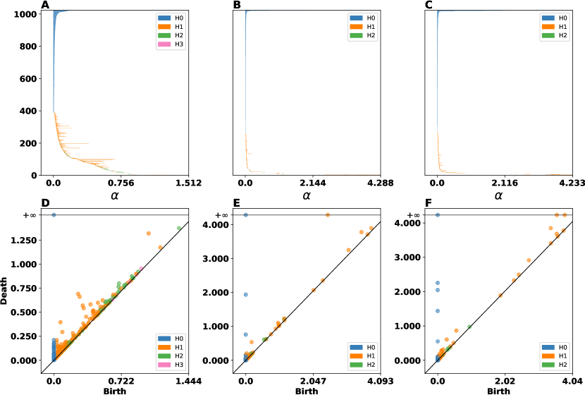
Furthermore, we performed the persistent homology to identify important topological features in the input space and investigate how well the SOM and RSOM captured those features. Figures 6A, B, and C show the persistent barcodes for the input space, SOM, and RSOM, respectively. We can see how the RSOM (panel C) captures more $H1$- and $H2$-homological properties (since there are more persistent line segments, orange and green lines). The SOM (panel B) seems to capture some of those features as well but they do not persist as long as they in the case of RSOM. The persistence diagrams of input, SOM and RSOM are shown in figures 6 D, E, and F, respectively. These figures indicate that the RSOM has more persistent features (orange and green dots away from the diagonal line) than the regular SOM. The Bottleneck distance between the persistence diagrams of input space and those of SOM and RSOM reveals that the SOM’s persistence diagram is slightly closer to the input space’s one for both the $H0$ (SOM: $0.00035$, RSOM: $0.0007$), $H1$ (SOM: $0.006$, RSOM: $0.007$), and $H2$ (SOM: $0.0062$, RSOM: $0.0057$). Despite the fact that the bottleneck distances show that regular SOM’s persistent diagram is closer to input space’s one, the barcodes diagrams indicate that the RSOM captures more persistent topological features suggesting that RSOM preserves in a better way the topology of the input space. Furthermore, the RSOM seems to capture better the higher dimensional topological features since the Bottleneck distances of $H2$-homological features are smaller for the RSOM than for the SOM.

Figure 5: Three dimensional uniform dataset (results) Randomized SOM made of $4096$ neurons with a $3$-nearest neighbors induced topology. Model has been trained for $25,000$ epochs on three-dimensional points drawn from a uniform distribution on the unit cube. A Map topology in neural space. B Map codeword in neural space. Each neural voronoi cell is painted with the color of the codeword. C to H Normalized distance map for six samples, respectively (1,1,1), (0,0,0), (1,1,0), (1,0,0), (0,1,0) and (0,0,1) in RGB notations. Normalization has been performed for each sample in order to enhance contrast but this prevents comparison between maps.

Figure 6: Three dimensional uniform dataset (analysis) Persistent Barcodes of A input space, B SOM, and RSOM. The blue, orange, and green line segments represent the $H0$-, $H1$-, and $H2$-homology, respectively. This means that blue color represents connected segments within the space and orange color reflects the holes within the space and the green one the voids. The longer the line segment the more important the corresponding topological feature. D illustrates the persistent diagram for the input space. E and F depict the persistent diagrams for SOM and RSOM, respectively. Again blue dots indicate $H0$-homology features, orange dots represent $H1$-homolocical features, and green the $H2$-homological features.

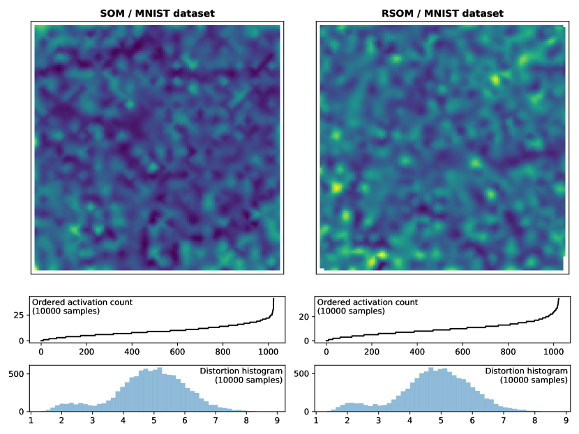
3.3 MNIST dataset

We tested RSOM on the standard MNIST dataset [29] that contains $60,000$ training images and $10,000$ testing images. The dimension of each image is 28$\times$28 pixels and they are encoded using grayscale levels as the result of the normalization of the original black and white NIST database. The standard performance on most algorithms on the MNIST dataset is below 1% error rate (with or without preprocessing) while for the regular SOM it is around 90% recognition rate depending on the initial size, learning rate, and neighborhood function. Our goal here is not to find the best set of hyper-parameters but rather to explore if SOM and RSOM are comparable for a given set of hyper-parameters. Consequently, we considered a size of 32$\times$32 neurons and used the entire training set (60,000 examples) for learning and we measured performance on the entire testing set. We did not use any preprocessing stage on the image and we fed directly each image of the training set with the associated label to the model. Labels (from 0 to 9) have been transformed to a binary vector of size 10 using one-hot encoding (e.g. label 3 has been transformed to 0000001000). These binary labels can then be learned using the same procedure as for the actual sample. To decode the label associated to a code word, we simply consider the argmax of these binary vectors. Figure 7 shows the final self-organisation of the RSOM where the class for each cell has been colorized using random colors. We can observe a number of large clusters of cells representing the same class (0, 1, 2, 3, 6) while the other classes (4,5,7,8,9) are split in two or three clusters. Interestingly enough, the codewords at the borders between two clusters are very similar. In term of recognition, this specific RSOM has an error rate just below 10% ($0.903,\,\pm 0.296$) which is quite equivalent to the regular SOM error rate ($0.906,\,\pm 0.292$). The perfomances of the RSOM and SOM are actually not significantly different, suggesting that the regular grid hypothesis can be weaken.

In a similar way we measured the similarity of the neural spaces generated by both the regular SOM and the RSOM using the persistent diagram and barcodes. The only significant difference from previous analysis was the projection of the input and neural spaces to a lower-dimension space via UMAP [33]. Projections of high-dimensional spaces to lower-dimension ones have been used before in the analysis of latent spaces of autoencoders [12]. Here, we use the UMAP since it’s an efficient and robust method for applying a dimensionality reduction on input and neural spaces. More precisely, we project the MNIST digits as well as the code words (dimension $784$) to a space of dimension $7$. Once we get the projections, we proceed to the topological analysis using the persistent diagram and barcodes as we already have described in previous paragraphs. Figure 8 shows the results regarding the persistent barcodes and diagrams. The persistent barcodes in figures 8A, B, and C indicate that RSOM captures more persistent features (panel C, orange and green lines reflect the $H1$- and $H2$-homological features, respectively) than the regular SOM (panel B). The persistence diagrams of input, SOM and RSOM are shown in figures 8 D, E, and F, respectively. These figures indicate that the RSOM has more persistent features (orange and green dots away from the diagonal line) than the regular SOM, consistently with the two previous experiments ($2$D uniform distribution with holes and $3$D uniform distribution). The Bottleneck distance between the persistence diagrams of input space and those of SOM and RSOM for the $H0$ are SOM: $1.0$ and RSOM: $1.12$, for $H1$ SOM: $0.19$ and RSOM: $0.22$, and finally for the $H2$ are SOM: $0.05$ and RSOM:$0.05$. Again we observe that the regular SOM has a persistent diagram that is closer to the one of the input space than that of RSOM, however the RSOM seems to approache slightly better the input space topology since it has more pairs (birth, death) away from the diagonal (black line) in figures 8D, E, and F. Moreover, the persistent barcode of RSOM (figure 8C indicates that has more persistent features for the radius $\alpha$ between $0$ and $1.512$ than the regular SOM.

Figure 7: MNIST dataset (results) Randomized SOM made of $1024$ neurons with a $3$-nearest neighbors induced topology. Model has been trained for $25,000$ epochs on the MNIST dataset. A Map topology in neural space. B Map topology in data space. C to H Normalized distance map for six samples. Normalization has been performed for each sample in order to enhance contrast but this prevents comparison between maps.

Figure 8: MNIST dataset (analysis) Persistent Barcodes of A input space, B SOM, and RSOM. The blue, orange, and green line segments represent the $H0$-, $H1$-, and $H2$-homology, respectively. This means that blue color represents connected segments within the space, orange color reflects the holes within the space and green the voids. The longer the line segment the more important the corresponding topological feature. D illustrates the persistent diagram for the input space. E and F depict the persistent diagrams for SOM and RSOM, respectively. Again blue dots indicate $H0$-homology features, orange dots represent $H1$-homolocical features, and green the $H2$-homological features.

3.4 Reorganization following removal or addition of neurons

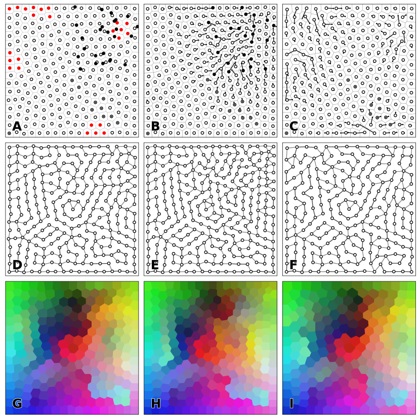
The final and most challenging experiment is to test how the RSOM can cope with degenerative cases, where either neurons die out (removal) or new units are added to the map (addition). Figure 9A illustrates an example of a well-formed neural space (black outlined discs), a removal (red disks) and an addition (black dots). For both removal and addition, we applied a LLoyd relaxation scheme to achieve a new quasi-centroidal Voronoi tesselation. Figures 9B and 9C depicts the Voronoi tesselations after $100$ iterations starting from the initial tesselation shown in panel 9A.

In order to conserve as much as possible the original topology, we used a differentiated procedure depending on if we are dealing with a removal or an addition. In case of removal, only the remaining neurons that were previously connected to a removed unit are allowed to connect to a new unit unconditionally. For the rest of the units, they might reconnect to a nearby unit if this unit is much closer than its closest current neighbour (85% of the smallest distance to its current neighbours). In case of addition, new units can connect unconditionally to the nearest neighbours while old unit can only connect to the newly added unit if this unit is much closer than its current closest neighbour (85% of the smallest distance to its current neighbours). This procedure guarantees that the topology is approximately conserved as shown in figures 9D-F. We tested the alternative of recomputing the graph from scratch but the resulting topology is quite different from the original because of micro-displacements of every units following the Lloyd relaxation.

Learning is performed in two steps. First we iterate $25,000$ epochs using the intact map, then we perform removal and addition and learning is iterated for another $5,000$ epochs for all three maps (orginal map, map with added units and map with removed units). The final self-organization is shown in figures 9G-I where we can observe strong similarities in the organization. For example, the central red patch is conserved in all three maps and the overall structure is visually similar. Of course, these results depend on the number of removed or added units (that needs to be relatively small compared to the size of the whole map) and their spatial distribution.

Figure 9: Reorganization (results). An initial set of 248 neurons (outlined discs on panel A) has been modified with the addition of 25 neurons (black discs) or the removal of 25 neurons (red discs). Panels B and C show the final position of neurons after 100 iterations of the centroidal Voronoi tesselation. Lines shows individual movement of neurons. Panels D, E and F show the 2-neighbors induced topology for A, B and C respectively. Panels G, H and I show the map map codebook for each map in neural space after learnin. Each voronoi cell of a neuron is painted with the color of the related codeword.

4 Discussion

We have introduced a variation of the self-organizing map algorithm by considering the random placement of neurons on a two-dimensional manifold, following a blue noise distribution from which various topologies can be derived. We’ve shown these topologies possess random (but controllable) discontinuities that allow for a more flexible self-organization, especially with high-dimensional data. This has been demonstrated for low-dimensional cases as well as for high-dimensional case such as the classical MNIST dataset [29]. To analyze the results and characterize properties within the maps, we used tools from the field of topological data analysis and random matrix theory that provide extra information when compared to regular quality measures [38]. More specifically, we computed the persistence diagrams and barcodes for both the regular and randomized self-organizing maps and the input space and we estimated the eigenvalues distributions of the Gram matrices for the activity of both SOMs. Overall, our results show that the proposed algorithm performs equally well as the original SOM and develop well-formed topographic maps. In some cases, RSOM preserves actually better the topological properties of the input space when compared to the original SOM but it is difficult to assert that this is a general property since a theoretical approach would be a hard problem. Another important aspect we highlighted is that RSOM can cope with the addition or the removal of units during learning and preserve, to a large extent, the underlying self-organization. This reorganization capacity allows to have an adaptive architecture where neurons can be added or removed following an arbitrary quality criterion.

This article comes last in a series of three articles where we investigated the conditions for a more biologically plausible self-organization process. In the first article [40], we introduced the dynamic SOM (DSOM) and showed how the time-dependent learning rate and neighborhood function variance of regular SOM can be replaced by a time-independent learning process. DSOM is capable of continuous on-line learning and can adapt anytime to a dynamic dataset. In the second article [13, 14], we introduced the dynamic neural field SOM (DNF-SOM) where the winner-take-all competitive stage has been replaced by a regular neural field that aimed at simulating the neural activity of the somatosensory cortex (area 3b). The whole SOM procedure is thus replaced by an actual distributed process without the need of any supervisor to select the BMU. The selection of the BMU as well as the neighborhood function emerge naturally due to the lateral competition between neurons that ultimately drives the self-organization. The present work is the last part of this sequel and provides the basis for developing biologically plausible self-organizing maps. Taken together, DSOM, DNF-SOM and RSOM provides a biological ground for self-organization where decreasing learning rate, winner-take-all and regular grid are not necessary. Instead, our main hypotheses are the blue noise distribution and the nearest-neighbour connectivity pattern. For the blue noise distribution and given the physical nature of neurons [6, 28], we think it makes sense to consider neurons to be at a minimal distance from each others and randomly distributed and to have a nearest-neighbour connectivity as it is known to occur in the cortex [45]. The case of reorganization, where neurons physically migrate (Lloyd relaxation), is probably the most dubious hypothesis but seems to be partially supported by experimental results [23]. It is also worth to mention that reorganization takes place naturally in the mammal brain. More precisely, neurogenesis happens in the subgranular zone of the dentate gyrus of the hippocampus and in the subventricular zone of the lateral ventricle [2]. On the other hand, when neural tissue in the cerebral cortex [34, 43] or the spinal cord [4, 30] are damaged, neurons reorganize their receptive fields and undamaged nerves sprout new connections and restore function (partially or fully). During such event, it has been shown that neurons can physically move.

Finally, the analysis we performed (TDA, eigenvalues distributions, distortion, and entropy indicates that both SOM and RSOM perform equally well. For the majority of the measures we used to assess the performance of both algorithms, we observed very similar results. Only in the case of TDA, we identified some differences in the topological features the two algorithms can capture. More precisely, both algorithms generate maps that capture most of the topological features of the input space. RSOM tends to capture slightly better high-dimensional topological features, especially for input spaces with holes (see the experiment on the $2D$ uniform distribution in Section 3.1). Therefore, we can conclude that the RSOM matches the performance of the SOM.

Abbreviations

BMU

Best Matching unit

DNF-SOM

Dynamic Neural Field-Self-Organizing Map

DSOM

Dynamic Self-organizing Map

KSOM

Kohonen Self-Organizing Map (Kohonen original proposal)

KDE

Kernel Density Estimation

RSOM

Randomized Self-Organizing Map

TDA

Topological Data Analysis

SOM

Self-Organizing Map

Funding

This work was partially funded by grant ANR-17-CE24-0036.

Appendix A Supplementary material

Randomized Self Organizing Map
Nicolas P. Rougier^1,2,3 and Georgios Is. Detorakis^4
1 Inria Bordeaux Sud-Ouest
² Institut des Maladies Neurodégénératives, Université de Bordeaux, CNRS UMR 5293
³ LaBRI, Université de Bordeaux, Institut Polytechnique de Bordeaux, CNRS UMR 5800
⁴ adNomus Inc., San Jose, CA, USA

Abstract. We propose a variation of the self organizing map algorithm by considering the random placement of neurons on a two-dimensional manifold, following a blue noise distribution from which various topologies can be derived. These topologies possess random (but controllable) discontinuities that allow for a more flexible self-organization, especially with high-dimensional data. The proposed algorithm is tested on one-, two- and three-dimensions tasks as well as on the MNIST handwritten digits dataset and validated using spectral analysis and topological data analysis tools. We also demonstrate the ability of the randomized self-organizing map to gracefully reorganize itself in case of neural lesion and/or neurogenesis.

A.1 One-dimensional uniform dataset

Figure 10: One dimensional uniform dataset with holes (results) Randomized SOM made of $1024$ neurons with a $3$-nearest neighbors induced topology. Model has been trained for $25,000$ epochs on one-dimensional points drawn from a uniform distribution on the unit segment. A Map topology in neural space. B Map topology in data space. C to H Receptive field of the map for six samples.

A.2 Two dimensional uniform dataset

Figure 11: Two dimensional uniform dataset (results) Randomized SOM made of $1024$ neurons with a $2$-nearest neighbors induced topology. Model has been trained for $25,000$ epochs on two-dimensional points drawn from a uniform distribution on the unit square. A Map topology in neural space. B Map topology in data space. C to H Receptive field of the map for six samples.

A.3 Two-dimensional ring dataset

Figure 12: Two dimensional ring dataset (results) Randomized SOM made of $1024$ neurons with a $3$-nearest neighbors induced topology. Model has been trained for $25,000$ epochs on two-dimensional points drawn from a ring distribution on the unit square. A Map topology in neural space. B Map topology in data space. C to H Normalized distance map for six samples. Normalization has been performed for each sample in order to enhance contrast but this prevents comparison between maps.

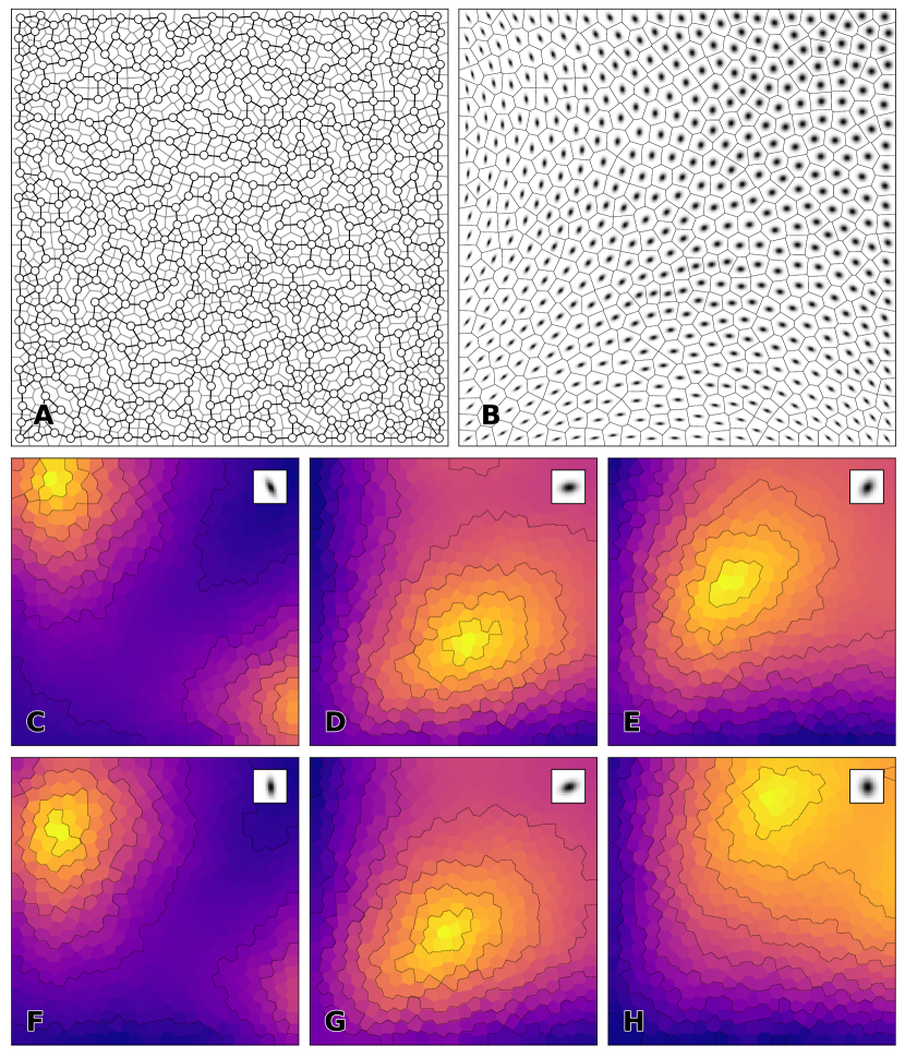
A.4 Oriented Gaussians dataset

Figure 13: Oriented Gaussians dataset (results) Randomized SOM made of $1024$ neurons with a $2$-nearest neighbors induced topology. Model has been trained for $25,000$ epochs on oriented Gaussian datasets. A Map topology in neural space. B Map topology in data space. C to H Receptive field of the map for six samples.

A.5 Influence of the topology

Figure 14: Influence of topology on the self organization. The same initial set of 1024 neurons has been equiped with 2-nearest neighbors, 3 nearest neighbors and 4-nearest neighbors induced topology (panels A, B and C respectively) and trained on 25,000 random RGB colors. This lead to qualitatively different self-organization as shown on panels D, E and F respectively, with major discontinuities in the 2-nearest neighbors case. ).

A.6 Eigenvalues distribution

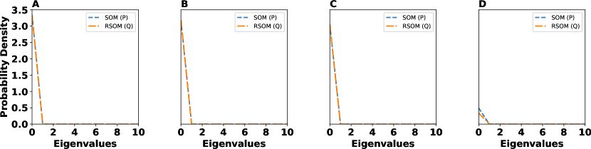
One way to investigate if there is any significant difference between the regular and random SOMs is to compare their neural responses to the same random stimuli. Therefore, we measure the neural activity and build a covariance matrix out of it. Then, we compute the eigenvalues of the covariance matrix (or Gram matrix) and we estimate a probability distribution. Thus, we can compare the eigenvalues distributions of the two maps and compare them to each other. If the distributions are close enough in the sense of Wasserstein distance then the two SOMs are similar in terms of neural activation. A Gram matrix is an $n\times n$ matrix given by where $n$ is the number of neurons of the map and ${\bf Y}\in\mathbb{R}^{n\times m}$ is a matrix for which each column is the activation of all $n$ neurons to a random stimulus.

From a computational point of view we construct the matrix ${\bf Y}$ by applying a set of stimuli to the self-organized map and computing the activity of each neuron within the map. This implies that ${\bf Y}\in\mathbb{R}^{m\times n}$, where $m=1024$ (the number of neurons) and $n={2,3}$ (two- or three-dimensional input samples). Then we compute the covariance or Gram matrix as ${\bf M}={\bf Y}{\bf Y}^{T}\in\mathbb{R}^{n\times n}$, where $n$ is the number of neurons. Then we compute the eigenvalues and obtain their distribution by sampling the activity of neurons of each experiment for $200$ different initial conditions using $50$ input sample each time. At the end of sampling we get an ensemble of $200$ Gram matrices and finally we estimate the probability density of the eigenvalues on each ensemble by applying a Kernel Density Estimation method [36] (KDE) with a Gaussian kernel and bandwidth $h=0.4$. This allows us to quantify any differences on the distributions of the regular and randomized SOMs by calculating the Earth-Mover or Wasserstein-1 distance over the two distributions (regular ($P$) and random SOM ($Q$)). The Wasserstein distance is computed as $W(P,Q)=\inf_{\gamma\in\Pi(P,Q)}\{\mathbb{E}_{(x,y)\sim\gamma}\Big{[}||x-y||\Big{]}\}$, where $\Pi(P,Q)$ denotes the set of all joint distributions $\gamma(x,y)$, whose marginals are $P$ and $Q$, respectively. Intuitively, $\gamma(x,y)$ indicates how much “mass” must be transported from $x$ to $y$ to transform the distribution $P$ into the distribution $Q$.

The distributions of the eigenvalues of the RSOM and the regular SOM are shown on figure 15. We can conclude that the two distributions are alike and do not suggest any significant difference between the two maps in terms of neural activity. This implies that the RSOM and the regular SOM have similar statistics of their neural activities. This means that the loss of information and the stretch to the input data from both RSOM and regular SOM are pretty close and the underlying topology of the two maps do not really affect the neural activity. This is also confirmed by measuring the Wasserstein distance between the two distributions. The blue curve shows the regular SOM or distribution $P$ and the black curve the RSOM or distribution $Q$. The Wasserstein distance between the two distributions $P$ and $Q$ indicates that the two distributions are nearly identical on all datasets. The Wasserstein distances in Table 2 confirm that the eigenvalues distributions of SOM and RSOM are almost identical indicating that both maps retain the same amount of information after learning the representations of input spaces.

Experiment	Wasserstein Distance
$2$D ring dataset	$0.0000323$
$2$D uniform dataset with holes	$0.0000207$
$3$D uniform dataset	$0.0001583$
MNIST dataset	$0.0015$

Table 2: Wasserstein distances of eigenvalues distributions. We report here the Wasserstein distances between eigenvalues distributions of SOM and RSOM for each of the four major experiments we ran. The results indicate that the distributions are close pointing out that the SOM and RSOM capture a similar level of information during training. For more information regarding how we computed the eigenvalues distributions and the Wasserstein distance please see Section A.6.

Figure 15: Eigenvalues distribution for A 2D Ring dataset B 2D uniform dataset with holes C 3D uniform dataset and D MNIST Dataset

A.7 Distortion and entropy measures

Figure 16: Two dimensional uniform dataset (measures). Measure of distortion and mean activation over 10,000 samples.

Figure 17: Two dimensional uniform dataset with holes (measures)Measure of distortion and mean activation over 10,000 samples.

Figure 18: Three dimensional uniform dataset (measures). Measure of distortion and mean activation over 10,000 samples.

Figure 19: MNIST dataset (measures). Measure of distortion and mean activation over 10,000 samples.

References

- [1] D. Alahakoon, S.K. Halgamuge, and B. Srinivasan. Dynamic self-organizing maps with controlled growth for knowledge discovery. IEEE Transactions on Neural Networks, 11(3):601–614, 5 2000.
- [2] Arturo Alvarez-Buylla and Daniel A Lim. For the long run: maintaining germinal niches in the adult brain. Neuron, 41(5):683–686, 2004.
- [3] César A. Astudillo and B. John Oommen. Topology-oriented self-organizing maps: a survey. Pattern Analysis and Applications, 17(2):223–248, 3 2014.
- [4] Florence M Bareyre, Martin Kerschensteiner, Olivier Raineteau, Thomas C Mettenleiter, Oliver Weinmann, and Martin E Schwab. The injured spinal cord spontaneously forms a new intraspinal circuit in adult rats. Nature neuroscience, 7(3):269–277, 2004.
- [5] Justine Blackmore and Risto Miikkulainen. Visualizing high-dimensional structure with the incremental grid growing neural network. In Machine Learning Proceedings 1995, pages 55–63. Elsevier, 1995.
- [6] Lidia Blazquez-Llorca, Alan Woodruff, Melis Inan, Stewart A. Anderson, Rafael Yuste, Javier DeFelipe, and Angel Merchan-Perez. Spatial distribution of neurons innervated by chandelier cells. Brain Structure and Function, 220(5):2817–2834, July 2014.
- [7] Robert Bridson. Fast poisson disk sampling in arbitrary dimensions. In ACM SIGGRAPH 2007 sketches on - SIGGRAPH '07. ACM Press, 2007.
- [8] Juan C. Burguillo. Using self-organizing maps with complex network topologies and coalitions for time series prediction. Soft Computing, 18(4):695–705, 11 2013.
- [9] Gunnar Carlsson. Topology and data. Bulletin of the American Mathematical Society, 46(2):255–308, 2009.
- [10] Frédéric Chazal and Bertrand Michel. An introduction to topological data analysis: fundamental and practical aspects for data scientists. arXiv preprint arXiv:1710.04019, 2017.
- [11] Pierre Demartines. Organization measures and representations of kohonen maps. In First IFIP Working Group, volume 10. Citeseer, 1992.
- [12] Georgios Detorakis, Travis Bartley, and Emre Neftci. Contrastive hebbian learning with random feedback weights. Neural Networks, 114:1–14, 2019.
- [13] Georgios Is. Detorakis and Nicolas P. Rougier. A neural field model of the somatosensory cortex: Formation, maintenance and reorganization of ordered topographic maps. PLoS ONE, 7(7):e40257, July 2012.
- [14] Georgios Is. Detorakis and Nicolas P. Rougier. Structure of receptive fields in a computational model of area 3b of primary sensory cortex. Frontiers in Computational Neuroscience, 8, July 2014.
- [15] Herbert Edelsbrunner and John Harer. Persistent homology-a survey. Contemporary mathematics, 453:257–282, 2008.
- [16] A.E. Eiben and J.E. Smith. Introduction to Evolutionary Computing. Springer Verlag, 2003.
- [17] Bernd Fritzke. A growing neural gas network learns topologies. In Proceedings of the 7th International Conference on Neural Information Processing Systems, NIPS’94, pages 625–632, Cambridge, MA, USA, 1994. MIT Press.
- [18] Robert Ghrist. Barcodes: the persistent topology of data. Bulletin of the American Mathematical Society, 45(1):61–75, 2008.
- [19] Suzana Herculano-Houzel, Charles Watson, and George Paxinos. Distribution of neurons in functional areas of the mouse cerebral cortex reveals quantitatively different cortical zones. Frontiers in Neuroanatomy, 7, 2013.
- [20] J. D. Hunter. Matplotlib: A 2d graphics environment. Computing In Science & Engineering, 9(3):90–95, 2007.
- [21] Fei Jiang, Hugues Berry, and Marc Schoenauer. The impact of network topology on self-organizing maps. In Proceedings of the first ACM/SIGEVO Summit on Genetic and Evolutionary Computation - GEC '09. ACM Press, 2009.
- [22] Eric Jones, Travis Oliphant, and Pearu Peterson. SciPy: Open source scientific tools for Python, 2001.
- [23] Naoko Kaneko, Masato Sawada, and Kazunobu Sawamoto. Mechanisms of neuronal migration in the adult brain. Journal of Neurochemistry, 141(6):835–847, April 2017.
- [24] Samuel Kaski, Jari Kangas, and Teuvo Kohonen. Bibliography of self-organizing map (som) papers: 1981-1997. Neural Computing Surveys, 1, 1998.
- [25] Teuvo Kohonen. Self-organized formation of topologically correct feature maps. Biological Cybernetics, 43(1):59–69, 1982.
- [26] Teuvo Kohonen. Self-Organizing Maps, volume 30 of Springer Series in Information Sciences. Springer-Verlag, Berlin, Germany, 3 edition, 2001.
- [27] Ares Lagae and Philip Dutré. A comparison of methods for generating poisson disk distributions. Computer Graphics Forum, 27(1):114–129, 3 2008.
- [28] Matteo Paolo Lanaro, Hélène Perrier, David Coeurjolly, Victor Ostromoukhov, and Alessandro Rizzi. Blue-noise sampling for human retinal cone spatial distribution modeling. Journal of Physics Communications, 4(3):035013, 2020.
- [29] Yann LeCun, Léon Bottou, Yoshua Bengio, and Patrick Haffner. Gradient-based learning applied to document recognition. Proceedings of the IEEE, 86(11):2278–2324, 1998.
- [30] Chan-Nao Liu and WW Chambers. Intraspinal sprouting of dorsal root axons: Development of new collaterals and preterminals following partial denervation of the spinal cord in the cat. AMA Archives of Neurology & Psychiatry, 79(1):46–61, 1958.
- [31] S. Lloyd. Least squares quantization in PCM. IEEE Transactions on Information Theory, 28(2):129–137, 3 1982.
- [32] Clément Maria, Jean-Daniel Boissonnat, Marc Glisse, and Mariette Yvinec. The gudhi library: Simplicial complexes and persistent homology. In International Congress on Mathematical Software, pages 167–174. Springer, 2014.
- [33] Leland McInnes, John Healy, and James Melville. Umap: Uniform manifold approximation and projection for dimension reduction. arXiv preprint arXiv:1802.03426, 2018.
- [34] Michael M Merzenich, Randall J Nelson, Michael P Stryker, Max S Cynader, Axel Schoppmann, and John M Zook. Somatosensory cortical map changes following digit amputation in adult monkeys. Journal of comparative Neurology, 224(4):591–605, 1984.
- [35] Merja Oja, Samuel Kaski, and Teuvo Kohonen. Bibliography of self-organizing map (som) papers: 1998-2001 addendum. Neural Computing Surveys, 3, 2003.
- [36] Emanuel Parzen. On estimation of a probability density function and mode. The annals of mathematical statistics, 33(3):1065–1076, 1962.
- [37] Fabian Pedregosa, Gaël Varoquaux, Alexandre Gramfort, Vincent Michel, Bertrand Thirion, Olivier Grisel, Mathieu Blondel, Peter Prettenhofer, Ron Weiss, Vincent Dubourg, et al. Scikit-learn: Machine learning in python. the Journal of machine Learning research, 12:2825–2830, 2011.
- [38] Daniel Polani. Measures for the organization of self-organizing maps. In Self-Organizing Neural Networks, pages 13–44. Physica-Verlag HD, 2002.
- [39] Matti Pöllä, Timo Honkela, and Teuvo Kohonen. Bibliography of self-organizing map (som) papers: 2002-2005 addendum. Helsinki University of Technology, 2009.
- [40] Nicolas P. Rougier. [Re] Weighted Voronoi Stippling. ReScience, 3(1), 2017.
- [41] Nicolas P. Rougier and Yann Boniface. Dynamic self-organising map. Neurocomputing, 74(11):1840–1847, 2011.
- [42] Joseph Rynkiewicz. Self organizing map algorithm and distortion measure, 2008.
- [43] Edward Taub, Gitendra Uswatte, and Victor W Mark. The functional significance of cortical reorganization and the parallel development of ci therapy. Frontiers in Human Neuroscience, 8:396, 2014.
- [44] Stéfan van der Walt, S Chris Colbert, and Gaël Varoquaux. The NumPy array: A structure for efficient numerical computation. Computing in Science & Engineering, 13(2):22–30, 3 2011.
- [45] Jaap van Pelt and Arjen van Ooyen. Estimating neuronal connectivity from axonal and dendritic density fields. Frontiers in Computational Neuroscience, 7, 2013.
- [46] Thomas Villmann. Topology preservation in self-organizing maps. In Kohonen Maps, pages 279–292. Elsevier, 1999.
- [47] Yahan Zhou, Haibin Huang, Li-Yi Wei, and Rui Wang. Point sampling with general noise spectrum. ACM Transactions on Graphics, 31(4):1–11, 7 2012.
- [48] Afra Zomorodian and Gunnar Carlsson. Computing persistent homology. Discrete & Computational Geometry, 33(2):249–274, 2005.