The SALT survey of helium-rich hot subdwarfs: methods, classification, and coarse analysis.

Abstract

A medium- and high-resolution spectroscopic survey of helium-rich hot subdwarfs is being carried out using the Southern African Large Telescope (SALT). Objectives include the discovery of exotic hot subdwarfs and of sequences connecting chemically-peculiar subdwarfs of different types. The first phase consists of medium-resolution spectroscopy of over 100 stars selected from low-resolution surveys. This paper describes the selection criteria, and the observing, classification and analysis methods. It presents 107 spectral classifications on the MK-like Drilling system and 106 coarse analyses ($\mbox{\,\em T${}_{\rm eff}$},\log g,\log y$) based on a hybrid grid of zero-metal non-LTE and line-blanketed LTE model atmospheres. For 75 stars, atmospheric parameters have been derived for the first time. The sample may be divided into 6 distinct groups including the classical ‘helium-rich’ sdO stars with spectral types (Sp) sdO6.5 - sdB1 (74) comprising carbon-rich (35) and carbon-weak (39) stars, very hot He-sdO’s with Sp $\lesssim$ sdO6 (13), extreme helium stars with luminosity class $\lesssim 5$ (5), intermediate helium-rich subdwarfs with helium class 25 – 35 (8), and intermediate helium-rich subdwarfs with helium class $10-25$ (6). The last covers a narrow spectral range (sdB0 – sdB1) including two known and four candidate heavy-metal subdwarfs. Within other groups are several stars of individual interest, including an extremely metal-poor helium star, candidate double-helium subdwarf binaries, and a candidate low-gravity He-sdO star.

1 Introduction

Hot subluminous stars can be divided into three major groups. These include i) the hydrogen-rich subdwarf B (sdB) stars, often characterized as extreme horizontal-branch stars, ii) the sdOB and sdO stars lying on or around the helium-main sequence, and iii) the more luminous sdO stars on post-AGB evolution tracks (Heber, 2016). Apart from the sdB stars which have hydrogen-rich surfaces, a substantial fraction of hot subdwarfs have hydrogen-deficient or hydrogen-weak surfaces. Amongst these, there is evidence for sequences extending either away from or towards the helium main-sequence, connecting with cooler extreme helium stars, or with the white dwarf cooling sequence; many have atmospheres enriched in carbon or nitrogen or both. Amongst the subdwarfs with hydrogen-weak surfaces, several show extraordinary overabundances of heavy metals (trans-iron elements) including zirconium and lead (Naslim et al., 2011, 2013). This diversity is apparent in the helium subclasses identified by Drilling et al. (2013) (D13 hereafter), who noted that certain classes of helium-rich hot subdwarf and extreme helium stars are difficult to distinguish at low resolution. In order to trace these sequences of hydrogen-deficient and hydrogen-weak subdwarfs with greater clarity, to discover how they relate to other categories of hydrogen-deficient star, and to study the physics that transforms their surface chemistries, we commenced a survey of chemically-peculiar hot subdwarfs. The object of the survey would be to obtain spectra of sufficient quality to measure effective temperature, surface gravities, and surface hydrogen, helium, carbon and nitrogen abundances, as well as to identify any exotic elements that might be present. This paper reports the initial part of the survey including selection criteria, observing procedures, data products and primary classifications.

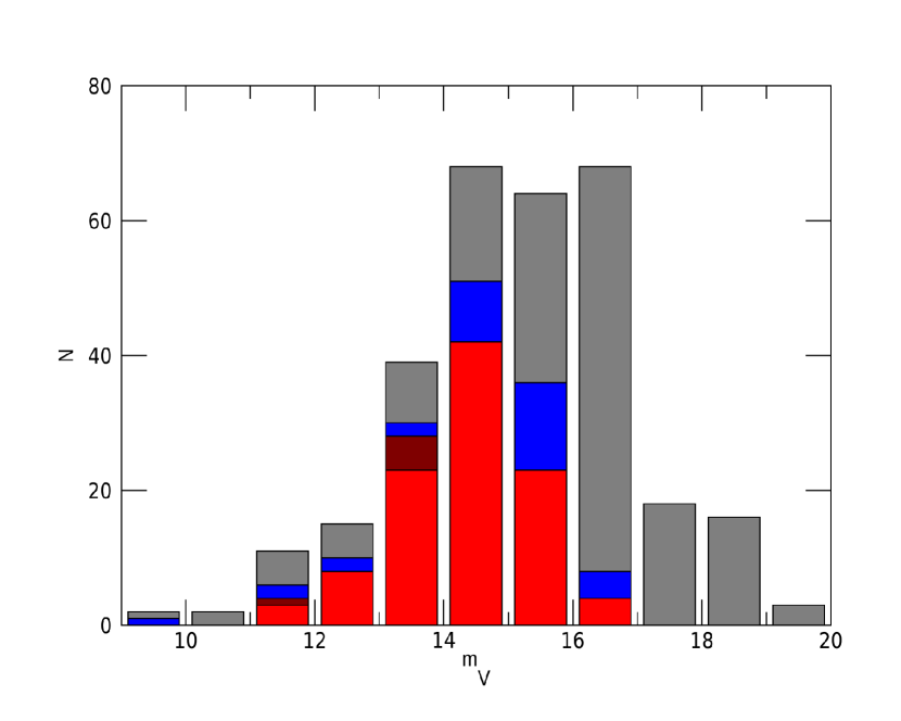
Figure 1: Relative numbers of known or suspected He-sdO, He-sdOB and He-sdB stars visible from SALT ordered by brightness. The coloured segments represent the numbers observed in the current sample with SALT/RSS only or with SALT/RSS and SALT/HRS (103 stars: red), with SALT/HRS only (6: dark red), or with another high-resolution spectrograph and not SALT (33: blue). As of 2020 September 30, the total known to us is 306.

2 Observations

2.1 Target selection

The primary motivation for this survey was the classification of several stars in the Edinburgh-Cape (EC) survey of faint blue stars as ‘He-sdB’ (Stobie et al., 1997a; Kilkenny et al., 1997), a classification similar to sdOD in the Palomar-Green (PG) survey (Green et al., 1986) and indistinguishable at the survey resolutions from that of ‘extreme helium stars’ (D13). Efforts to explore this category by Ahmad & Jeffery (2003) and by Naslim et al. (2010) were limited by telescope aperture and observing time. The construction of the Southern African Large Telescope (SALT) offered the perfect opportunity to extend previous studies.

Initial target selection was made on the basis of low-resolution classifications of He-sdB, He-sdOB and He-sdO in the EC survey. These classifications are described by Moehler et al. (1990b); Geier et al. (2017) and Lei et al. (2020). To these were added similar stars classified He-sdB, sdOD, or similar in one or more of the compilations by Carnochan & Wilson (1983); Green et al. (1986); Kilkenny & Lynas-Gray (1982); Kilkenny (1988); Beers et al. (1992); Stobie et al. (1997a); Kilkenny et al. (1997); Adelman-McCarthy et al. (2006); Østensen (2006); Németh et al. (2012); O’Donoghue et al. (2013); Kilkenny et al. (2015); Kepler et al. (2015); Kilkenny et al. (2016) or Geier et al. (2017). Stars which had been observed at high resolution with échelle spectrographs at either VLT/UVES (Ströer et al., 2007), AAT/UCLES (Ahmad et al., 2007; Naslim et al., 2011, 2012), ESO/FEROS (Naslim et al., 2013), or Subaru/HDS (Jeffery et al., 2017b; Naslim et al., 2020) were not included at first, but the benefits of having medium resolution spectra available for class prototypes meant that some were included later.

Since the boundaries between He-sdB, He-sdOB and He-sdO are spectroscopic and therefore artificial in terms of exploring connections between stars in closely related classes, stars from all three categories were included as the survey progressed. Moreover, since some chemically-peculiar subdwarfs simply have solar or slightly super-solar abundances of helium, we included a number of sdOB and sdO stars. The principal exclusions were stars classified sdB, since these usually have weak or absent Hei and no Heii lines.

Our helium-rich list currently (2020 September) contains over 600 subdwarfs, of which $306$ lie between the declinations of $-75^{\circ}$ and $+8^{\circ}$, the effective limits of SALT. Some 33 of the latter have been observed at high resolution in campaigns cited above and are not included here. Approximately 30 are common to previous campaigns and to the SALT observations presented here. Figure 1 shows the brightness distribution of known or suspected southern helium-rich subdwarfs accessible to SALT.

Table 1: Observation dates in the form yyyymmdd. The full table is given in the Supplementary Online Data.

Name	RSS Dates	HRS Dates
Ton S 144	20181101	20180611
Ton S 148	20191101	20180616 20180705 20180722 20190619 20190715
…	…	…

2.2 SALT/HRS

From 2016 to the present, observations have been obtained with the SALT High Resolution Spectrograph (HRS: $R\approx 43\,000$, $\lambda\lambda=4100-5200$Å, Bramall et al., 2010). Observation dates are given in Table 1. HRS spectra obtained prior to 2019 were reduced to order-by-order wavelength calibrated rectified form using the SALT pipeline pyHRS (Crawford et al., 2016); orders were stitched into a single spectrum using our own software. In general, spectra were obtained in pairs (or a higher multiple) which were coadded to provide a single observation for each date. The pyHRS pipeline ceased to be supported after the beginning of 2019. HRS spectra obtained after that date will be described in a subsequent paper.

2.3 SALT/RSS

To reduce errors arising from poor blaze correction, which is difficult for broad-lined spectra, and also to extend the sample to stars too faint for HRS, observations were also obtained with the SALT Robert Stobie Spectrograph (RSS: resolution $R\approx 3\,600$, Burgh et al. (2003); Kobulnicky et al. (2003)). Observation dates are given in Table 1. Since the RSS detector consists of three charge-coupled devices separated by two gaps, double exposures were taken at two different grating angles. This provides a continuous spectrum in the wavelength range 3850 – 5150 Å  and assists in the removal of cosmic-ray contamination. Basic data processing used the pysalt package (Crawford et al., 2010). Reduction used standard iraf tasks and the lacosmic package (van Dokkum, 2001) as described by Koen et al. (2017). The one-dimensional wavelength-calibrated and sky-subtracted spectra were extracted using the apall task. These were rectified using low-order polynomials fitted to regions of continuum identified automatically. The three segments from both observations at both grating angles were merged using weights based on the number of photons detected in each segment. The wavelengths of each spectrum were adjusted to correct for Earth motion.

2.4 The Drilling sample

The complete sample of normalised spectra used by D13 (the ‘Drilling sample’) has been used to validate the classification procedure.

2.5 Nomenclature

The SALT sample is described in Table 3.2, which gives positions (J2000.0), Gaia magnitudes, names, and classifications. By convention, we adopt the catalogue name at which the star was first identified as a helium-rich subdwarf. Other catalogues which include the star are indicated by abbreviation; a full list is available for each star from simbad (Wenger et al., 2000). For brevity, we have contracted BPS CS to BPS and, except in Table 3.2, the full GALEX identifier to GLX Jhhmmm+ddmm, with positions rounded down to tenths of a minute in right ascension and arcminutes in declination.

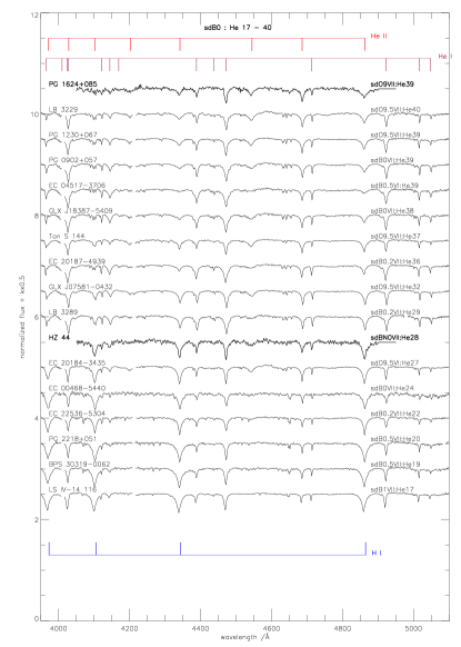
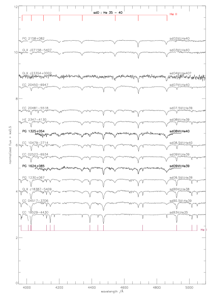
Figure 2: SALT atlas of early-type helium-rich hot subdwarfs showing (left) helium classes from He17 to He40 at spectral type around sdB0 and (right) spectral types from sdO2 to sdB3 with helium class 38 – 40 that do not show strong C or N lines. Principal lines are indicated in colour. In some cases star names are obvious contractions of names given in Table 2. Bold labels and spectra represent standards from D13.

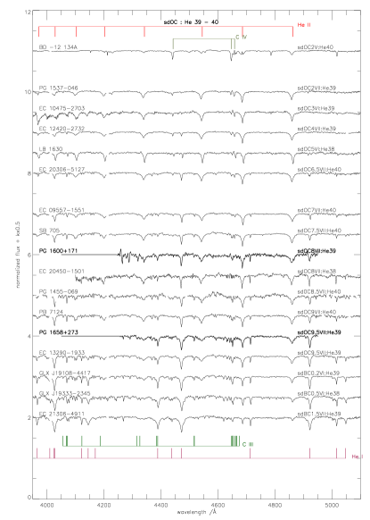
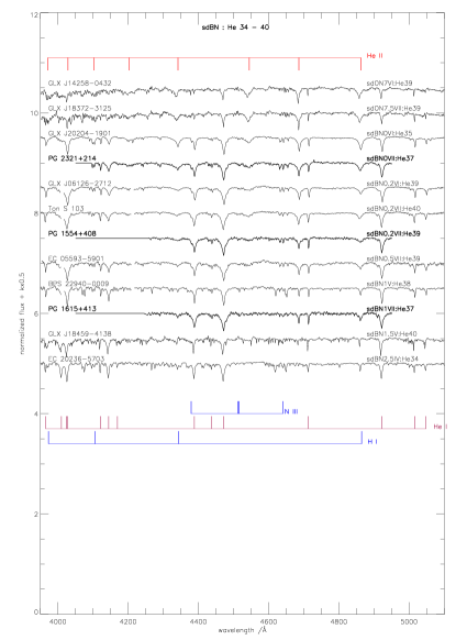
Figure 3: As Fig. 2 for (left) C-rich subdwarfs with spectral types from sdOC2 to sdBC1.5 with helium class 38 – 40 and (right) N-rich subdwarfs with spectral types from sdON7 to sdBN2.5 with helium class 34 – 40.

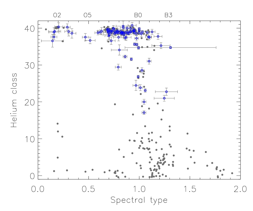
Figure 4: The Sp – He classification diagram for helium-rich subdwarfs (blue circles). The distribution from D13 is shown by grey dots; a uniform jitter covering $\pm$ half a division has been applied to both datasets in both axes.

3 Classification

3.1 Method

Classification using the D13 system gives proxies for effective temperature  $T_{\rm eff}$ (spectral type), surface gravity $g$ (luminosity class), and helium / hydrogen ratio $y$ (helium class). The criteria for spectral type and helium class are based on relative line strengths and depths assuming a spectral resolution $R\approx 2\,000$. Both HRS and RSS spectra are therefore degraded to this resolution for classification.

Spectral type, luminosity class and helium class are evaluated numerically from the digital spectra. For helium class (He) formulae based on fractional line depths $d$ are given by D13:

$${\rm He}<20:\\ {\rm He}=20*(d_{4471}+d_{4541})/(d_{\gamma}-0.83d_{4541})$$

$${\rm He}\geq 20:\\ {\rm He}=40-20*(d_{\gamma}-0.83d_{4541})/(d_{4471}+d_{4541})$$

Spectral types (Sp) for helium-rich classes are based on Hei/Heii line ratios as follows:

$$d_{4686}\geq d_{4471}:{\rm Sp}=0.1+0.8d_{4471}/d_{4686},$$

$$d_{4686}<d_{4471}:{\rm Sp}=0.9+0.4(1-d_{4686}/d_{4471}).$$

Sp corresponds to a numerical scale on which spectral type O2 = 0.2, O5 = 0.5, B0 = 1.0, etc. D13 derived spectral types for hydrogen-rich classes using the depths of H$\beta$ ($d_{\beta}$) and H$\gamma$ ($d_{\gamma}$). For helium classes He $<12$ and spectral types later than O8, we define:

$${\rm Sp}=((3.8d_{\gamma}-0.5)+(4.8d_{\beta}-0.8))/2.$$

Table 2: Line depth criteria for He-strong stars to be sub-classified C or N.

C	Civ 4658 $|$ 4442	$d>0.08$
C	Ciii 4647 $|$ 4650	$d>0.10$
C	Cii 4267 $|$ 4619	$d>0.13$
N	Niii 4379 $|$ 4513 $|$ 4640	$d>0.09$
N	Nii 4530 $|$ 4447	$d>0.20\,\,\&\,\,{\rm Sp}>1.0$

Luminosity classes are harder to quantify from simple line criteria. Line widths for gravity-sensitive lines were calibrated against spectral type and helium class using the sample of spectra from D13, and used with partial success.

Criteria for identifying carbon- and nitrogen-strong spectra were established by measuring depths of carbon and nitrogen lines for stars identified as sdOC and sdBN by D13. Criteria valid for He-strong spectra (He$>25$) are summarized in Table 2

Errors are based on the signal-to-noise in each spectrum estimated from a region of continuum and then propagated formally through the line depth formulae.

Figures comparing automatic classification of the Drilling sample with the D13 manual classifications are shown in Appendix A.

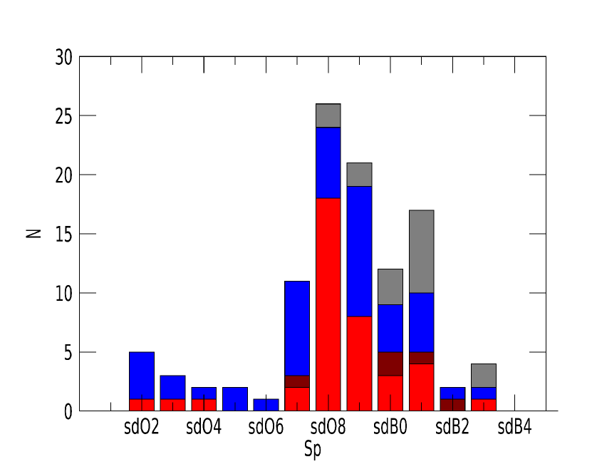
Figure 5: The distribution of SALT helium-rich subdwarf stars by spectral type. Coloured segments represent stars in helium class He$\geq 35$, subdivided into carbon-rich (C: blue), nitrogen-rich (N: maroon) and no qualification (red). Stars with He $<35$ are enumerated in grey. The total number of stars in the sample is 106.

3.2 Results

To achieve sufficient signal-to-noise for subsequent analysis, spectra for several stars were obtained over more than one observing block. Originally, the reduced spectrum from each block was classified as a separate spectrum, which gave a good indication of the errors associated with noise. The final classification was obtained from a single spectrum constructed from all SALT/RSS observations combined. Where an RSS spectrum was not available, the weighted average HRS spectrum was degraded by convolution with a Gaussian FWHM = 1.2Å. This is essential because the relative depths of broad and sharp lines change with spectral resolution. Final classifications are shown in Table 3.2. The prefix ‘sd’ implies a D13 classification as distinct from an MK classification; it does not of itself imply that the object is a subdwarf. Fig. 4 shows the spectral-type helium-class distribution obtained from automatic SALT classifications. The distribution of the sample by spectral type is shown in Fig., 5. Both Figs. 4 and 5 suggest a break in the distribution at spectral type sdO6. One may identify a minimum of three groups containing stars with: a) spectral type earlier than sdO6 (all have helium class $\geq 35$), b) helium class $<35$ (and spectral types between sdO9 and sdB1), and c) those having helium class $\geq 35$ and spectral type between sdO6 and sdB3. These groups include all but two or three outliers. By further considering the luminosity class, it may be shown that other groups exist. However, errors currently associated with the luminosity criteria determine that other physical characteristics associated with the spectra should be examined first.

Although there are 58 stars with He$\geq 15$ in D13, only 7 are common to the SALT sample. The majority of the D13 sample are northern hemisphere stars. The latter range from spectral type sdO2 to sdB1, from luminosity class VI to VIII, and from helium class He18 to He40. In six, the differences are less than one subclass in spectral type, luminosity class and helium class. The seventh is sdO2 in D13 and sdO4 here.

Table 3: Fundamental data and classifications for helium-rich hot subdwarfs observed with SALT.

FUNDAMENTAL DATA			NAMES		LORES		SALT		CLASS	Notes
$\alpha_{2000}$	$\delta_{2000}$	$m_{G}$	Adopted	Other	Class	Ref
00:10:07	$-$26:12:56	12.8	Ton S 144	PHL, SB, FB, MCT, BPS, EC	HesdB sdO6He4	EC5 lam00	RSS	HRS	sdO9.5VII:He37
00:18:53	$-$31:56:02	14.4	Ton S 148	PHL, HE, MCT, GLX, EC	HesdB sdO7He3	EC5 lam00	RSS	HRS	sdBC0.2VI:He37
00:49:05	$-$54:24:39	16.2	EC 00468$-$5440		HesdB	EC5	RSS		sdBC0VII:He24
01:16:53	$-$22:12:09	14.8	BPS 22946$-$0005	MCT	B, pAGB	BPS	RSS		sdB2.5II:He24
01:43:08	$-$38:33:16	13.0	SB 705	GLX, EC	HesdO	kil89	RSS	HRS	sdOC7.5VII:He40
01:47:17	$-$51:33:39	13.5	LB 3229	JL, GLX	HesdO	kil89	RSS	HRS	sdO9.5VII:He39
02:10:54	$+$01:47:47	13.7	Feige 19	PB, PG, GLX	HesdO	moe90	RSS	HRS	sdO9VII:He37	D13
02:33:26	$-$59:12:31	15.1	LB 1630	EC	HesdO	EC5	RSS		sdOC5VI:He38
02:43:23	$+$04:50:36	14.1	PG 0240+046	GLX	sdOB	PG	RSS	HRS	sdBC0.5VII:He25	D13
02:51:21	$-$72:34:33	14.6	LB 3289	EC, GLX	HesdO	EC3	RSS	HRS	sdB0.2VII:He30
02:52:51	$-$69:22:34	16.1	EC 02523$-$6934		HesdO	EC4	RSS		sdO9VII:He39
03:06:08	$-$14:31:52	15.6	PHL 1466	PB, EC	HesdO	EC5	RSS		sdOC4V:He40	noisy
03:50:38	$-$69:20:57	14.7	EC 03505$-$6929		HesdO	EC4	RSS		sdO9VII:He40
04:03:05	$-$40:09:41	14.4	EC 04013$-$4017		HesdB	EC5	RSS	HRS	sdBC1VII:He32
04:11:10	$-$00:48:48	14.1	GLX J041110.1$-$004848		HesdO	ØG	RSS	HRS	sdO8VII:He40
04:13:19	$-$13:41:03	12.5	EC 04110$-$1348		HesdO	EC3	RSS		sdOC7.5VII:He39
04:15:30	$-$54:21:59	14.9	HE 0414$-$5429	EC, GLX	HesdO	ØG	RSS		sdO8VII:He39
04:20:35	$+$01:20:41	12.3	GLX J042034.8+012041		HesdO	ven11	RSS	HRS	sdOC8.5VII:He40
04:22:37	$-$54:08:50	14.0	LB 1721	EC, GLX	HesdO	EC4	RSS		sdOC9VII:He38
04:29:11	$-$29:02:48	14.1	EC 04271$-$2909	BPS, GLX	HesdO	BPS	RSS		sdO8.5VI:He39
04:29:33	$-$47:31:44	15.8	EC 04281$-$4738	GLX	sdB?	EC4	RSS		sdOC6.5VII:He39
04:36:15	$-$53:43:34	12.5	LB 1741	EC	HesdO	kil92	RSS		sdO9VII:He39
04:37:34	$-$61:57:43	14.6	BPS 29520$-$0048	EC, GLX	HesdO	rod07	RSS		sdOC9VII:He39
04:42:26	$-$32:06:01	14.8	EC 04405$-$3211	GLX	HesdO	EC4	RSS		sdO7.5VII:He39
04:53:32	$-$37:01:43	15.7	EC 04517$-$3706		HesdB	EC3	RSS		sdB0.5VI:He40
05:13:48	$-$19:44:18	15.1	GLX J051348.2$-$194417		HesdOB	ØG	RSS		sdO7.5VII:He39
05:17:57	$-$30:47:50	13.3	Ton S 415	EC, GLX	HesdO	EC3	RSS	HRS	sdO8VII:He30
05:26:12	$-$28:58:25	15.6	EC 05242-2900	GLX	HesdB	EC3	RSS		sdOC7VII:He39
05:58:05	$-$29:27:09	15.2	GLX J055804.5$-$292708		HesdOB	ØG	RSS		sdOC7VII:He39
06:00:01	$-$59:01:03	16.1	EC 05593$-$5901		HesdB	EC3	RSS		sdBN0.5VII:He39
06:12:37	$-$27:12:55	13.4	GLX J061237.5$-$271254		HesdOB	ØG	RSS	HRS	sdBN0.2VI:He40
07:07:39	$-$62:22:41	14.5	GLX J070738.9$-$622241		HesdOB	ØG	RSS	HRS	sdOC6.5VII:He40
07:15:50	$-$54:07:57	14.4	GLX J071549.6$-$540755		HesdO	ØG	RSS	HRS	sdO3VII:He40
07:58:08	$-$04:32:05	13.1	GLX J075807.5$-$043203		HesdO	nem12	RSS	HRS	sdO9.5VII:He33
08:35:24	$-$01:55:53	11.4	[CW83] 0832$-$01		sdOp	CW83	RSS		sdO8VII:He40
08:45:29	$-$12:14:10	14.0	GLX J084528.7$-$121410		HesdOB	ØG	RSS	HRS	sdOC9.5VI:He39
09:05:05	$+$05:33:01	14.1	PG 0902+057	GLX	sdOD	PG	RSS	HRS	sdB0VII:He39	D13
09:07:08	$-$03:06:14	11.9	[CW83] 0904$-$02		sdOp(He)	ber80	RSS		sdO7.5VI:He39
09:18:56	$-$57:04:25	12.9	LSS 1274		HesdO	ØG	RSS		sdOC8VI:He39
09:58:11	$-$16:05:52	14.3	EC 09557$-$1551	BPS, GLX	HesdO	EC2	RSS		sdO7VII:He40
10:00:43	$-$12:05:59	14.0	PG 0958$-$119	HE, EC, GLX	HesdO	EC2	RSS		sdO8VI:He39
10:49:55	$-$27:19:09	13.4	EC 10475$-$2703	GLX	HesdO	EC2		HRS	sdOC3VII:He39
10:50:18	$-$27:30:37	13.9	EC 10479$-$2714	GLX	HesdO	EC2	RSS		sdO8.5VII:He40
11:26:11	$-$20:01:39	14.4	EC 11236$-$1945	GLX	HesdO	EC2	RSS		sdOC2VII:He40
11:30:04	$+$01:37:37	13.8	PG 1127+019	GLX	sdOD	PG	RSS	HRS	sdOC9.5VII:He39	D13
12:22:59	$-$05:53:05	14.7	PG 1220$-$056	GLX	sdOC	PG	RSS		sdO4VII:He39	D13
12:33:23	$-$06:25:18	13.1	PG 1230+067	GLX		PG	RSS		sdON9.5VII:He39	D13
12:37:35	$-$28:41:01	14.8	EC 12349$-$2824	GLX	HesdO	EC2	RSS		sdO8VII:He40
12:44:42	$-$27:48:58	14.7	EC 12420$-$2732	GLX	HesdO	EC2	RSS		sdOC4VII:He40
13:20:44	$+$05:59:01	14.7	PG 1318+062		sdOC	PG	RSS	HRS	sdOC9VI:He39
13:31:46	$-$19:48:26	14.4	EC 13290$-$1933	GLX	HesdB	EC2	RSS		sdOC9.5VII:He39	sen15
14:25:50	$-$04:32:33	14.0	GLX J142549.8$-$043231		HesdOB	ØG		HRS	sdO9VII:He39
14:57:57	$-$07:05:05	16.4	PG 1455$-$069		sdOB	PG	RSS		sdOC8.5VII:He40
15:23:32	$-$18:17:26	13.9	GLX J152332.2$-$181726		HesdOB	ØG	RSS	HRS	sdCO9VII:He39
15:30:56	$+$02:42:23	15.4	PG 1528+029	GLX	sdOC	PG	RSS		sdO8VII:He40
15:37:40	$-$17:02:15	15.1	EC 15348$-$1652	GLX	HesdO	EC2	RSS		sdO8VII:He39
15:40:33	$-$04:48:12	15.0	PG 1537$-$046	BPS, GLX	HesdO	PG	RSS		sdOC2VII:He40	D13
16:28:36	$-$03:32:38	15.5	PG 1625$-$034	BPS, GLX	HesdO	BPS	RSS		sdO8VII:He39	noisy
16:54:38	$+$03:18:47	15.1	GLX J165438.5+031847		HesdO	ØG	RSS		sdOC3VII:He40
17:05:06	$-$71:56:09	13.8	GLX J170506.0$-$715609		HesdO	ØG	RSS	HRS	sdO7.5VII:He39
18:32:32	$-$47:44:38	13.5	GLX J183231.7$-$474435		HesdOB	ØG		HRS	sdOC9VII:He38
18:37:17	$-$31:25:16	13.9	GLX J183716.7$-$312514		HesdOB	ØG		HRS	sdO7.5VII:He39

Table 4: continued

Fundamental Data: $\alpha_{2000}$, $\delta_{2000}$, $m_{G}$: Gaia Collaboration (2018), 1: EC3 ($m_{V}$). Selected catalogues: BPS=Beers et al. (1992), [CW83]=Carnochan & Wilson (1983), ${\rm EC}={\rm EC}n:n=1,5=$Stobie et al. (1997b); Kilkenny et al. (1997); O’Donoghue et al. (2013); Kilkenny et al. (2015); Kilkenny et al. (2016), Feige=Feige (1958), FB=Greenstein & Sargent (1974), GLX=Bianchi et al. (2017), HE=Wisotzki et al. (1996), JL=Jaidee & Lyngå (1969), KUV=Kondo et al. (1984), LB=(Luyten, 1953, et seq.), LS IV=Nassau & Stephenson (1963), LSS=Stephenson & Sanduleak (1971), MCT=Demers et al. (1990), PB=Berger & Fringant (1980a), PG=Green et al. (1986), PHL=Haro & Luyten (1962), SB=Slettebak & Brundage (1971), Ton S=Chavira (1958), UVO=Carnochan & Wilson (1983) LORES references: as above plus ber80=Berger & Fringant (1980b), ØG=Østensen (2006); Geier et al. (2017), kil89=Kilkenny & Muller (1989), kil92=Kilkenny & Busse (1992), lam00=Lamontagne et al. (2000), moe90=Moehler et al. (1990a), rod07=Rodríguez-López et al. (2007), str07=Ströer et al. (2007), ven11=Vennes et al. (2011), vit91=Viton et al. (1991) Notes. a CLASS has also given by: D13=Drilling et al. (2013), sen15=Şener-Şatir (2015), jef17=Jeffery (2017), nas11=Naslim et al. (2011) vos07=Voss et al. (2007); metal poor = very weak metal lines; noisy = too noisy to classify.

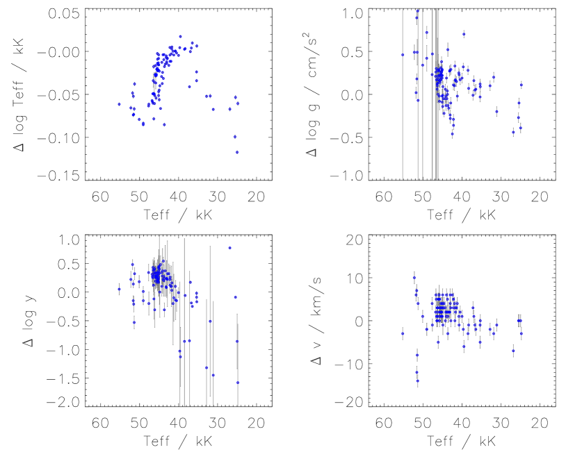
Figure 6: Residuals in the sense salt_p00 – XTgrid for  T_eff, $\log g$, $\log y$ and $v$ as functions of  T_eff. Offscale error bars are due to fit failures with salt_p00 at high  T_eff and with XTgrid at low  T_eff and $y$.

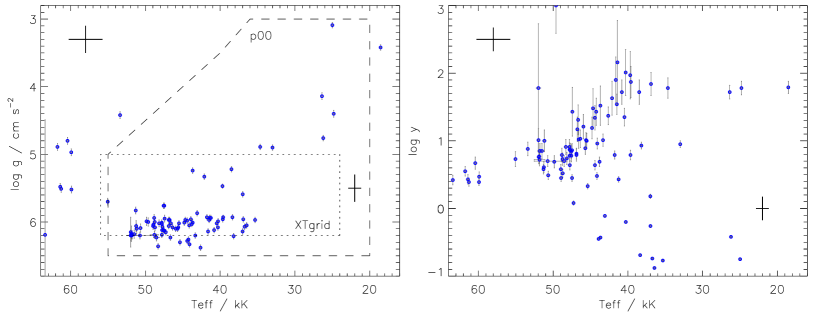
Figure 7: $\mbox{\,\em T${}_{\rm eff}$}-\log g$ (left) and $\mbox{\,\em T${}_{\rm eff}$}-\log y$ (right) diagrams for helium-rich subdwarfs from the SALT sample obtained from the salt_p00 model grid. The long-dashed line shows the boundary of the LTE solar-mix grid. The short-dashed line shows the boundary of the non-LTE zero-metal grid (Németh et al., 2012). Gray error bars associated with each datum are formal errors as given in Table 4.2. Stars with $\delta\log g>2$ are omitted. Dark error bars upper-left and lower-right represent estimated mean observational errors (see text).

4 Physical properties

4.1 Model atmospheres

An alternative to classification is to match observed spectra within a grid of theoretical spectra (models) in order to estimate physical properties pertaining to the atmosphere of each star. Here, these comprise the star’s effective temperature  T_eff, surface gravity $g$ and $y\equiv\mbox{\,$n_{\rm He}$}/\mbox{\,$n_{\rm H}$}$, the ratio of hydrogen to helium atoms by number.

Ideally, such models should also match the abundances of other significant chemical species, carbon, nitrogen and iron all having significant effects on the stellar spectrum. To minimize computational costs, the present study considers only the following grids:

salt_p00: models were computed with the Armagh LTE radiative transfer package lte-codes (Jeffery et al., 2001; Behara & Jeffery, 2006) on a grid:

$$\begin{split}\mbox{\,$T_{\rm eff}$}/{\rm kK}&=[08(01)16(02)40(02.5)55],\\ \mbox{\,$\log g/{\rm cm\,s^{-2}}$}&=[1.50(0.25)6.50],\\ \mbox{\,$n_{\rm He}$}&=[0.01,0.05,0.10,0.3,0.5,0.7,0.8,0.9,0.99,1.0].\end{split}$$

Emergent spectra were computed on a self-adapting wavelength grid which optimally samples the local opacity structure and yields between 50 000 and 200 000 wavelength points in the range 3500 – 6800 Å. The abundance distribution for elements heavier than helium based was assumed to be solar; hence the label p00 which is shorthand for +0.0 dex. In the course of this investigation, it was realised that the abundance normalisation within sterne, the model atmosphere component of lte_codes, assumed conservation of relative number fractions for metals when replacing hydrogen by helium. It is more natural that relative mass fractions should be conserved following, say, the fusion of 4 protons to a ${}^{4}{\rm He}$ nucleus. sterne was consequently modified and the entire model grid, currently comprising $\sim 4000$ models for a single metallicity and microturbulent velocity ($v_{\rm turb}$), was recomputed. For the latter, $v_{\rm turb}=0\,\mbox{$\mbox{km}\,\mbox{s}^{-1}$}$ was assumed for both the calculation of line opacities in the model atmosphere (which affects the temperature stratification of the models) and for the formal solution, which affects relative line strengths and widths. For comparison with the SALT RSS spectra, a subset of these models having

$$\begin{split}\mbox{\,$T_{\rm eff}$}/{\rm kK}&=[20,24,28,32,36,40,42.5,45,47.5,50,55],\\ \mbox{\,$\log g/{\rm cm\,s^{-2}}$}&=[3.0,3.5,4.0,4.5,5.0,5.5,6.0,6.5],\\ \mbox{\,$n_{\rm He}$}&=[0.3,0.5,0.7,0.9,0.99,1.0]\end{split}$$

was sampled over the wavelength interval $3600-5200$Å on an interval 0.2Å.

XTgrid: models computed with the non-LTE radiative transfer codes tlusty and synspec (Hubeny et al., 1994) for the analysis of hot subdwarfs observed in the Sloan Digital Sky Survey (Vennes et al., 2011; Németh et al., 2012) were made available by Nemeth et al. (2014). The original grid was defined as

$$\begin{split}&[\mbox{\,$T_{\rm eff}$}/{\rm kK},\mbox{\,$\log g/{\rm cm\,s^{-2}}$},\log y]\\ &=[20(1)56,5.0(0.1)6.2,-5.0(0.3)+2.0],\end{split}$$

with no contribution from elements heavier than helium, and a microturbulent velocity $v_{\rm turb}=0\,\mbox{$\mbox{km}\,\mbox{s}^{-1}$}$ throughout. This grid contains some 1390 model spectra each computed on a wavelength range 3130 - 7530 Å with typically 38  000 wavelength points. To conserve memory a subset having

$$\begin{split}\mbox{\,$T_{\rm eff}$}/{\rm kK}&=[24,28,32,36,40,44,48,52,56],\\ \mbox{\,$\log g/{\rm cm\,s^{-2}}$}&=[5.0,5.3,5.6,5.9,6.2],\\ \log y&=[-1.0,-0.4,+0.2,+0.8,+1.4,+2.0]\\ \end{split}$$

was sampled over the wavelength interval $3600-5200$Å on an interval 0.2Å(as above).

Ideally, the model atmosphere and emergent spectrum would be adapted and iterated to match the heavy-element distribution, and microturbulent velocity measured on a first iteration, since these strongly influence the atmosphere structure at low hydrogen abundances. At present, a full fine analysis is only practical for limited numbers of stars. For this paper, only approximate values are required in order to identify overall trends and stars of interest for further analysis. The LTE approximation is known to break down increasingly for stars with $\mbox{\,\em T${}_{\rm eff}$}\gtrsim 30\,000$ K, but is less important than the contribution of metal opacities otherwise (Anderson & Grigsby, 1991; Löbling, 2020). These systematics are also discussed for restricted cases by Napiwotzki (1997); Latour et al. (2011); Pereira (2011); Latour et al. (2014) and Schindewolf et al. (2018b). Chemical stratification due to radiative levitation provides an additional vector of free parameters not considered in the current models (Behara & Jeffery, 2008).

4.2 Method

lte_codes include the optimization code sfit (Jeffery et al., 2001). Here we use the Levenburg-Marquardt option to minimize the square residual between each observed normalized spectrum and the grid of models described above.

Before optimization, the radial velocity $v_{\rm rad}$ of the observed spectrum relative to the laboratory rest-frame is established by cross-correlation with a representative theoretical spectrum; the wavelengths of the observed spectrum are then corrected by this amount so that the radial velocity is not a free parameter of the fit.

Inputs to the optimization include the normalized spectrum shifted to the local rest-frame velocity, a definition of regions of spectrum representative of continuum, masks to exclude non-stellar features (e.g. interestellar calcium H and K), masks to give additional weight to key lines, full-width half-maximum for the instrumental broadening profile (1.25Å), and a threshold for excluding cosmic-ray features ($1.5\times$continuum). Regions of spectrum weighted 10 times other regions included H$\beta$, H$\gamma$, Heii 4686 and 4540 Å, Hei 4471, 4381, 4121, 4144 and 4169 Å.

The initial optimisation commences with starting values for $\mbox{\,\em T${}_{\rm eff}$}=33.0$kK, $\log g/{\rm cm\,s^{-2}}=4.9$, $n_{\rm He}=0.9$ and with the projected rotation velocity fixed at $\mbox{\,$v\,\sin i$}=0$. Two renormalization steps are carried out using the high-pass procedure outlined by Jeffery et al. (1998), with filter widths set at 200Å and 50Å respectively. An optimization step is carried out after each renormalization; for the second of these  $v\,\sin i$ is free.

Outputs from the optimization include  T_eff, $\log g$, $n_{\rm He}$ (or equivalently, $\log y=n_{\rm He}/n_{\rm H}$), and  $v\,\sin i$, as well as the renormalized observed and best-fit model spectra. $v_{\rm rad}$ determined prior to optimization is included in the overall set of outputs.

Various sets of starting values for  T_eff, $\log g$, and $n_{\rm He}$ were investigated. The adopted values were chosen because a converged solution was obtained in all cases. Choosing  T_eff too high or too low yielded consistent solutions in some fraction of cases, but also led to divergence for a fraction of late or early-type spectra, respectively.

Care is required in the choice of template used to determine $v_{\rm rad}$, especially for very hot stars. Because of the offset between hydrogen Balmer lines and He ii lines, a template helium-hydrogen ratio which does not match the observed spectrum produces a systematic velocity shift and hence degrades the model optimisation. A second iteration was therefore introduced in which the first best-fit model was used as the velocity template, the second $v_{\rm rad}$ measurement being retained.

From experience, the zero-points for both RSS and HRS wavelength calibrations must be treated with caution. Undocumented evidence for seasonal drifts might be associated with thermal drift in RSS, which sits on the tracker some 15 m above the primary mirror assembly. Early implementations of the HRS calibration pipeline suffered zero-point errors (Crawford, private communication). Consequently individual measurements of $v_{\rm rad}$ should be treated with caution. Excessively high values may indicate an object of interest.

Since  $v\,\sin i$ is an output from sfit, and required to ensure the solution is self-consistent, it has a lower limit represented by the instrumental resolution. For RSS spectra, $c/R\approx 83\,\mbox{$\mbox{km}\,\mbox{s}^{-1}$}$. For stars with $\mbox{\,\em T${}_{\rm eff}$}\gtrsim 50$ kK, there are no sharp lines in the zero-metal models with which to constrain the rotational broadening; hence  $v\,\sin i$ is degenerate with $\log g$. For the sample of 71 RSS spectra with $\mbox{\,\em T${}_{\rm eff}$}<50$ kK, $\langle\mbox{\,$v\,\sin i$}\rangle=83\pm 22\,\mbox{$\mbox{km}\,\mbox{s}^{-1}$}$, all except EC 20111–6902 have $\mbox{\,$v\,\sin i$}<\langle\mbox{\,$v\,\sin i$}\rangle+2\sigma$.

For the HRS spectra, the nominal $c/R\approx 7\,\mbox{$\mbox{km}\,\mbox{s}^{-1}$}$ was degraded by resampling so that the mean $\langle\mbox{\,$v\,\sin i$}\rangle=12\pm 2\,\mbox{$\mbox{km}\,\mbox{s}^{-1}$}$ obtained for four (excluding EC 10475–2703) using the line-blanketed LTE models is satisfactory. Again the absence of sharp lines in the high- T_eff zero-metal models required that $\mbox{\,$v\,\sin i$}=12\,\mbox{$\mbox{km}\,\mbox{s}^{-1}$}$ be fixed for the final fits.

Table 5: Atmospheric parameters for helium-rich hot subdwarfs observed and classified with SALT/RSS. Stars observed only with SALT/HRS are marked ’$\ast$’, $\sigma$ represents standard deviation of fluxes about the mean in a continuum region $\lambda 4810-4845$Å (i.e. $\sigma=0.01\Rightarrow{\rm S/N}=100$.) All errors are formal; rather, mean errors $\delta\mbox{\,\em T${}_{\rm eff}$}/\mbox{\,\em T${}_{\rm eff}$}\approx\pm 0.028$, $\delta\log g\approx\pm 0.27$, $\delta\log y\approx\pm 0.29$, and $\delta v_{\rm rad}\approx\pm 3.0\,\mbox{$\mbox{km}\,\mbox{s}^{-1}$}$ should be adopted (§ 4.3). For cases where sfit finds $\mbox{\,$n_{\rm He}$}\geq 1$, we set $\mbox{\,$n_{\rm He}$}=1$ and $\log y=3$. Tests suggest $\langle\delta v_{\rm rad}\rangle\approx\pm 3\,\mbox{$\mbox{km}\,\mbox{s}^{-1}$}$ (see tex). $v_{\rm wid}$ is a nominal measure of the line broadening, dominated by the instrumental width $c/R\approx 83\,\mbox{$\mbox{km}\,\mbox{s}^{-1}$}$ (RSS) (see text); a smaller value $\sim 12\,\mbox{$\mbox{km}\,\mbox{s}^{-1}$}$ is indicated where only an HRS spectrum is available (marked !).

Table 6: continued

4.3 Results

Values for  T_eff, $\log g$ and $\log y$ obtained for the full sample are shown in Table 4.2. Results lying outside respective grid boundaries are included for completeness. It is emphasized that these analyses have been carried out for the purpose of data exploration and discovery; their used in detailed investigations of individual stars may be ill advised.

Large errors in $\log y$ occur for stars with very low hydrogen abundances. The hydrogen abundance is difficult to measure precisely in hot helium-rich stars since the Balmer lines are completely dominated by the corresponding lines in the Heii Pickering series and, since $y\equiv\mbox{\,$n_{\rm He}$}/\mbox{\,$n_{\rm H}$}$, the increasing error in the smaller denominator dominates the error budget.

Table 4.2 also provides an estimate of the noise $\sigma$ in the spectrum used for the analysis, the radial velocity $v_{\rm rad}$ of said spectrum, and the parameter obtained as $v\sin i$ in the model atmosphere fit, but more precisely labelled as a line width $v_{\rm wid}$ in velocity units.

Fig. E.1 in the Supplementary Material shows correlations between physical parameters and spectral class indicators. Trends illustrate the systematics, and scatter provides an estimate of the random errors.

For $\mbox{\,\em T${}_{\rm eff}$}\lesssim 35$ kK, (Sp $\gtrsim$ sdB1) stars have surface gravities outside the XTgrid boundary; the salt_p00 grid results shown in Table 4.2 are to be preferred. For $42\gtrsim\mbox{\,\em T${}_{\rm eff}$}/{\rm kK}\gtrsim 35$ (sdO9 $\lesssim$ Sp $\lesssim$ sdB1), both grids give comparable values for  T_eff, with salt_p00 giving slightly higher $g$ (by 0 – 0.3 dex) for $\mbox{\,\em T${}_{\rm eff}$}\lesssim 42$ kK and lower $g$ for $\mbox{\,\em T${}_{\rm eff}$}\gtrsim 42$ kK. For $42\gtrsim\mbox{\,\em T${}_{\rm eff}$}/{\rm kK}\gtrsim 35$ (sdO9.5 $\lesssim$ Sp $\lesssim$ sdB1), salt_p00 gives $g$ higher than XTgrid by $\approx 0.1$ dex, but for $\mbox{\,\em T${}_{\rm eff}$}/{\rm kK}\gtrsim 42$ (Sp $\lesssim$ sdO9.5), systematic trends appear in the residual. For $\mbox{\,\em T${}_{\rm eff}$}\gtrsim 42$ kK (Sp $\lesssim$ sdO9.5), salt_p00 increasingly underestimates  T_eff compared with XTgrid. The latter provides a roughly linear correlation between  T_eff and Sp between sdO7 and sdB1, although the gradient is markedly steeper than the equivalent relation reported by D13. The differences between results obtained from the two model grids are shown in Fig. 6. These are indicative of the systematic errors introduced by assuming the overall metallicity and/or local thermodynamic equilibrium.

Experiments suggested that model grid spacings, metallicity and microturbulent velocity have a significant influence on the outcomes, but we conclude that the systematic errors introduced by the LTE assumption are unacceptable for $\mbox{\,\em T${}_{\rm eff}$}\geq 42$ kK. To avoid this critical boundary, we therefore use the nLTE zero metal grid (XTgrid) for $\mbox{\,\em T${}_{\rm eff}$}\geq 41$ kK. Below this value, metal-line blanketing and a model grid which extends to $\log g=3$ are both required to obtain satisfactory fits, so the salt_p00 grid is used for $\mbox{\,\em T${}_{\rm eff}$}<41$ kK. Excluding outliers, there is a mean offset of $\approx 1.3\pm 3.0\,\mbox{$\mbox{km}\,\mbox{s}^{-1}$}$ between radial velocities obtained using models from the two grids.

sfit provides formal errors on the parameters governing the fit used based on a value of $\chi^{2}$ which is not realistic because of the method used to increae the weight of specified spectral lines as described above. From the scatter of points in Fig. 6, we estimate measurement errors to be $\delta\log\mbox{\,\em T${}_{\rm eff}$}\approx\pm 0.012$, $\delta\log g\approx\pm 0.27$, $\delta\log y\approx\pm 0.29$, and $\delta v_{\rm rad}\approx\pm 3.0\,\mbox{$\mbox{km}\,\mbox{s}^{-1}$}$. For convenience, the first three translate to fractional errors: $\delta\mbox{\,\em T${}_{\rm eff}$}/\mbox{\,\em T${}_{\rm eff}$}\approx\pm 0.028$, $\delta g/g\approx\pm 0.62$, and $\delta y/y\approx\pm 0.67$. These should be used in preference to the formal errors cited in Table 4.2.

A second approach to estimating the measurement errors was to use the best-fit models obtained with the salt_p00 grid as an independent low-noise sample with otherwise similar spectral properties to the observed sample. This sample was processed with the XTgrid models in exactly the same way as before, except that no velocity correction was necessary. Then the differences between the parameters obtained from the observed sample and the theoretical sample were formed, giving the following mean differences and standard deviations: $\langle\Delta\log\mbox{\,\em T${}_{\rm eff}$}\rangle=0.000\pm 0.017$, $\langle\Delta\log g\rangle=0.253\pm 0.203$, and $\langle\Delta\log y\rangle=-0.112\pm 0.262$. Restricting the test sample to $\mbox{\,\em T${}_{\rm eff}$}>42$ kK, these numbers change to $\langle\Delta\log\mbox{\,\em T${}_{\rm eff}$}\rangle=-0.005\pm 0.015$, $\langle\Delta\log g\rangle=0.236\pm 0.201$, and $\langle\Delta\log y\rangle=-0.069\pm 0.174$. Again, these translate to mean fractional errors $\delta\mbox{\,\em T${}_{\rm eff}$}/\mbox{\,\em T${}_{\rm eff}$}\approx\pm 0.039$, $\delta g/g\approx\pm 0.46$, and $\delta y/y\approx\pm 0.40$.

Figure 8: RSS spectra and best fit solutions for a selection of representative stars. Each panel shows the merged spectrum (black histogram) and the best-fit solution (red polyline). The residual (observed – calculated) is plotted beneath. Each star’s identifier, assigned spectral type and physical parameters ( T_eff/kK, $\log g/{\rm cm\,s^{-2}}$, and $\log y$) are indicated, with formal errors in the last 2 digits in parentheses. Positions of hydrogen Balmer lines (red) and neutral helium lines (blue) are identified for EC 20236-5703. Ionized helium lines are identified for EC 1240-2732. ‘Continuum’ regions used to rectify all observed spectra are identified by blue crosses for the latter two stars. Equivalent plots for the entire sample of Table 3 are provided in the supplementary material.

Solutions obtained with both grids show a correlation between the upper limit of $\log y$ and  T_eff for $\mbox{\,\em T${}_{\rm eff}$}\mathrel{\raise 1.16pt\hbox{$>$}\kern-7.0pt\lower 3.06pt\hbox{{$\scriptstyle\sim$}}}40$kK (Fig. 7). As  T_eff increases and the number of neutral hydrogen atoms becomes critically small, RSS spectra containing helium become increasingly degenerate in $y$ at high  T_eff. The situation ameliorates at high resolution when the displacement between Balmer and ionized helium lines allows the former to be resolved.

Representative spectra and best-fit solutions are illustrated in Fig. 3.2. Equivalent plots for the entire sample of Table 3 are provided in Figs. E.1–E.7 of the Supplementary material.

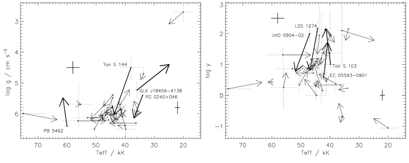
Figure 9: As Fig. 7, showing previous results for SALT sample members (grey error bars) linked to the current result (Table 4.2) by an arrow. The largest differences are indicated by thicker lines and labelled (i.e. for $\delta\log\mbox{\,\em T${}_{\rm eff}$}>0.1,\delta\log g>0.6,$ or $\delta\log y>1.0$). The mean SALT error bars are shown as in Fig. 7. Data values and sources for the previous results are given in the Supplementary Material (Appendix F). Where $g$ or $y$ were not given in the earlier study, we have substituted values from Table 4.2.

Table 7: Published atmospheric parameters for SALT sample members. Errors $<\pm 0.1$ have been rounded up.

Star	Teff		$\log g$		$\log y$		Reference
	kK		cm s-2
Ton S 144	38.0$\pm$	3.5	4.5$\pm$	0.4	0.4$\pm$	0.2	Hunger et al. (1981)
— " —	41.7$\pm$	1.1	5.7$\pm$	0.1	2.1$\pm$	0.1	Ströer et al. (2007)
BPS 22946–0005	20.0$\pm$	3.0	2.7$\pm$	0.3	–1.1$\pm$	0.1	Kendall et al. (1997)
SB 705	45.1$\pm$	8.1	5.6$\pm$	0.6	1.0$\pm$	0.4	Németh et al. (2012)
— " —	44.7$\pm$	3.5	5.8$\pm$	0.4	0.0$\pm$	0.1	Hunger et al. (1981)
LB 3229	40.0$\pm$	0.5	5.2$\pm$	0.2	1.9$\pm$	0.8	Naslim et al. (2010)
Feige 19	40.0$\pm$	2.5	5.0$\pm$	0.3	1.0$\pm$	1.5	Dreizler et al. (1990)
— " —	45.0$\pm$	2.5	6.0$\pm$	0.3	0.3$\pm$	0.4	Thejll et al. (1994)
PG 0240+046	37.0$\pm$	2.5	5.3$\pm$	0.3	0.1$\pm$	0.3	Thejll et al. (1994)
— " —	34.0$\pm$	0.2	5.4$\pm$	0.1	0.2$\pm$	0.1	Ahmad & Jeffery (2003)
EC 03505–6929	42.6$\pm$	0.2	6.2$\pm$	0.1	0.2$\pm$	0.1	Moni Bidin et al. (2017)
HE 0414–5429	50.6$\pm$	0.7	6.5$\pm$	0.1	0.3$\pm$	0.3	Moni Bidin et al. (2017)
GLX J04205+0120	45.0$\pm$	0.8	5.7$\pm$	0.2	$>1.2$		Vennes et al. (2011)
— " —	46.1$\pm$	0.9	6.0$\pm$	0.2	1.0$\pm$	0.2	Németh et al. (2012)
EC 04271–2909	53.0		–		–		Drilling & Beers (1995)
EC 05593–5901	42.2$\pm$	0.3	5.6$\pm$	0.2	0.6$\pm$	0.2	Moni Bidin et al. (2017)
GLX J07581–0432	41.4$\pm$	0.5	5.9$\pm$	0.3	0.5$\pm$	0.5	Németh et al. (2012)
PG 0902+057	43.0$\pm$	2.5	6.0$\pm$	0.3	1.5$\pm$	0.4	Thejll et al. (1994)
UVO 0904–02	47.0$\pm$	0.5	5.7$\pm$	0.1	2.0$\pm$	0.3	Schindewolf et al. (2018a)
LSS 1274	44.3$\pm$	0.4	5.5$\pm$	0.1	2.2$\pm$	0.3	Schindewolf et al. (2018a)
PG 0958–119	44.2$\pm$	0.5	5.4$\pm$	0.1	1.2$\pm$	0.4	Hirsch & Heber (2009)
PG 1127+019	43.7$\pm$	0.7	5.9$\pm$	0.2	1.9$\pm$	1.2	Luo et al. (2016)
PG 1230+067	43.0$\pm$	2.5	5.5$\pm$	0.3	1.2$\pm$	1.5	Thejll et al. (1994)
PG 1318+062	44.6$\pm$	1.0	5.8$\pm$	0.2	1.1$\pm$	0.8	Luo et al. (2016)
GLX J18459–4138	35.9$\pm$	4.8	5.2$\pm$	0.3	2.1$\pm$	1.1	Németh et al. (2012)
— " —	26.2$\pm$	0.8	4.2$\pm$	0.1	2.0$\pm$	0.4	Jeffery (2017)
GLX J19111–1406	56.0$\pm$	4.5	5.7$\pm$	0.7	0.3$\pm$	0.9	Németh et al. (2012)
BPS 22940–0009	33.7$\pm$	0.8	4.7$\pm$	0.2	2.2$\pm$	0.1	Naslim et al. (2010)
LS IV–14 116	34.0$\pm$	0.5	5.6$\pm$	0.1	–0.7$\pm$	0.1	Naslim et al. (2011)
— " —	35.0$\pm$	0.3	5.9$\pm$	0.1	–0.6$\pm$	0.1	Green et al. (2011)
— " —	35.2$\pm$	0.1	5.9$\pm$	0.1	–0.6$\pm$	0.1	Randall et al. (2015)
— " —	35.5$\pm$	1.0	5.9$\pm$	0.9	–0.6$\pm$	0.1	Dorsch et al. (2020)
PG 2158+082	75.1$\pm$	7.6	6.0$\pm$	0.2	0.2$\pm$	1.1	Németh et al. (2012)
BPS 22892–0051	45.7		–		–		Beers et al. (1992)
BPS 22875–0002	56.2		–		–		Beers et al. (1992)
PG 2218+051	36.5$\pm$	1.0	6.2$\pm$	0.2	–0.8$\pm$	0.1	Saffer et al. (1994)
— " —	36.0$\pm$	0.7	5.9$\pm$	0.1	–0.7$\pm$	0.1	Luo et al. (2016)
EC 22536–5304	36.9$\pm$	0.1	6.1$\pm$	0.1	–0.5$\pm$	0.1	Jeffery & Miszalski (2019)
Ton S 103	39.8$\pm$	3.5	6.5$\pm$	0.4	2$\pm$	1	Hunger et al. (1981)
PB 5462	47.5		8.2		–		Kepler et al. (2015)
— " —	60.0$\pm$	0.9	6.4$\pm$	0.1	–		Hügelmeyer et al. (2006)
HE 2347–4130	44.9$\pm$	1.2	5.8$\pm$	1.5	1.4$\pm$	0.4	Ströer et al. (2007)

4.4 Previous results

Spectroscopic measurements of one or more of $\mbox{\,\em T${}_{\rm eff}$},\log g,\log y$ have been published for some 30 members of the overall sample (Table 7). Fig. 9 compares those data with values in Table 4.2. More than two thirds of the differences are within either the errors of the original observations or of the new measurements. Of the remainder: PB 5462 (Hügelmeyer et al., 2006) lies outside the current model grid, Ton S 144 and Ton S,103 were measured using a restricted grid of nLTE models (Hunger et al., 1981), the weakness of He ii 4686 in GLX J18459–4138 was overlooked by Németh et al. (2012) (cf. Jeffery, 2017), the hydrogen abundances measured from high-resolution spectra of LSS 1274 and UVO 0904–02 by Schindewolf et al. (2018b) are to be preferred, the published helium abundance of EC 05593–5901 was 1.5 dex above the boundary of the model grid used by Moni Bidin et al. (2017), and the spectrum of PG 0240+046 used by Ahmad & Jeffery (2003) was limited to H$\gamma$, He i4388 and 4471.

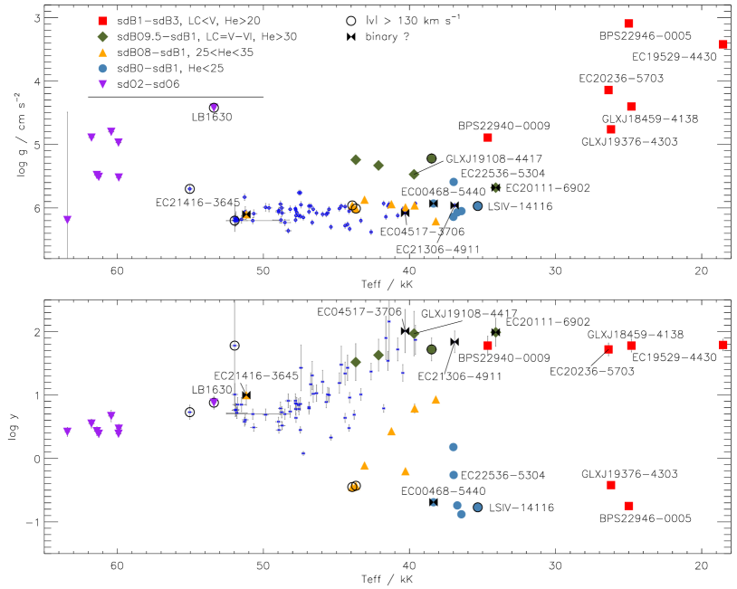
Figure 10: As Fig. 7 extended to identify subgroups and individual stars discussed in § 5. The groups identified in the key and by different colours and symbols correspond to §§ 5.1 – 5.7. The small blue circles refer to the remaining stars (cf. § 5.8).

5 Highlights

The primary objective of this part of the survey was to identify stars of particular interest for further investigation. For us this means: a) stars at late spectral types (sdO9–sdB3) (or low  T_eff and $g$) which might indicate links to other classes of helium-rich stars, b) stars with intermediate helium classes (He10–He35) (or helium - to - hydrogen ratios) which might include heavy-metal stars and confronts the question of why hot subdwarfs are predominantly extremely helium-poor or helium-rich, c) stars with anomalous radial or rotational velocities which might indicate subdwarfs in close binary systems or otherwise high-velocity stars. The stars have been gathered into subgroups described in the following subsections. Within each group, stars are introduced by name, spectral class and model-dependent parameters as in Table 4.2. The last are expressed as ($\mbox{\,\em T${}_{\rm eff}$}/{\rm kK},\log g/{\rm cm\,s^{-2}},\log y$). Groups and individual stars are identified in Fig. 10.

5.1 Sp = sdB1 – sdB3, LC $\lesssim$V, He $>20$

The first group includes stars which are classified sdB1 or later and have luminosity class V or less. These are indicated by filled red squares in Fig. 10. As such, they are not true subdwarfs since their surface gravity is similar to or lower than that of the main-sequence. Some or all might be shown to be subluminous on account of their mass and luminosity.

GLX J18459–4138 (sdB2V:He38)

(24.8, 4.4, 1.8) was identified as being similar to the pulsating helium star V652 Her. The survey parameters are consistent with those given by Jeffery (2017). It is the only nitrogen-rich member of this group.

GLX J19376–4303 (sdB2.5V:He21)

(26.2, 4.8, –0.4) appears similar to GLX J18459–4138 but has stronger Balmer lines, indicating hydrogen and helium abundances of 63% and 27% respectively (Jeffery et al., 2017a).

EC 19529–4430 (sdB3IV:He35)

(18.5, 3.4, 1.8) shows no ionized helium lines (including Heii 4686Å) and Balmer lines much weaker than the neutral helium lines. A defining feature is the weakness of all metal lines (cf. HD144941: Harrison & Jeffery, 1997) and the narrow wings of the H and Hei lines.

EC 20236–5703 (sdBC2.5IV:He35)

(26.4, 4.1, 1.7) has similar properties to EC 19529-4430, but with slightly narrower He i lines and a carbon rich metal-lined spectrum. It is likely to have similarities to the carbon-rich pulsating helium star BX Cir (Woolf & Jeffery, 2000).

BPS 22940–0009 (sdBC1V:He38)

(34.7, 4.9, 1.8) makes the fifth and hottest member of this group, all of which could be called extreme helium stars. Its closest well-studied counterparts are the hot extreme helium star LS IV$+6^{\circ}2$ (Jeffery, 1998), and PG 1415+492 (sdBC1VI:He39 Ahmad & Jeffery, 2003) and and PG 0135+243 (Moehler et al., 1990b). A high-resolution spectral analysis was carried out by Naslim et al. (2010) who showed it to be the lowest gravity member of their sample of helium-rich subdwarfs. Our coarse analysis is in general agreement.

BPS 22946–0005 (sdB2.5II:He24)

(25.0, 3.1, –0.8) has He $<30$ but otherwise fits this group. It is a post-AGB star analyzed by Kendall et al. (1997). It was mistakenly included in our sample but provides a useful control. In comparison with Kendall et al., our temperature is high and our gravity low, but still consistent with a post-AGB star.

5.2 Sp = sdO9.5 – sdB1, LC $\approx$ V – VI, He $>30$

If signal-to-noise ratios were higher, and luminosity classification was a more precise science, this section would isolate other sample members with LC $\leq$ VI, and hence identify the remaining high luminosity stars. Given the large errors associated with assigning luminosity class, $\log g\lesssim 5.7$ has been used as a proxy.

GLX J19108-4417 (sdBC0.2VI:He39)

(39.7, 5.5, 2.0) is just slightly hotter and less luminous than BPS 22940–0009 (see above). Whilst it also resembles the extreme helium dwarf LS IV$+6^{\circ}2$ (Jeffery, 1998), it has a higher hydrogen abundance (Beliere, 2018). Again, connections with PG 1415+492 (Ahmad & Jeffery, 2003) and PG 0135+243 (Moehler et al., 1990b) should also be explored.

Other stars in this group

include: EC 20111–6902 (sdBC1.5VII:He38 — 34.1, 5.7, 2.0), Ton S 148 (sdBC0.2VI:He37 – 38.5, 5.2, 1.7), GLX J08454–1214 (sdOC9.5VI:He39 — 43.4, 5.2, 1.5), and EC20221-6249 (sdOC9.5VII:He39 — 42.1, 5.3, 1.6). They are indicated by green diamonds in Fig. 10 and all await detailed analysis from high-resolution spectroscopy. These stars will be crucial in establishing any link between the low-luminosity helium stars identified in § 5.1 and helium-rich subdwarfs stars on the helium-main-sequence, such as the post-double white dwarf merger connection proposed by Zhang & Jeffery (2012).

Figure 11: As Fig. 3.2 for intermediate helium subdwarfs. LS IV$-14^{\circ}116$ and EC 22536-5304 are known heavy-metal subdwarfs (Naslim et al., 2010; Jeffery & Miszalski, 2019); PG 0240+046, PG 2218+051, BPS 30319–0062, or EC 00468–5440 have similar  T_eff  $g$ and $y$, but no heavy-metal detections yet.

5.3 Sp = sdB0 – sdB1, He $<25$

As a primary indicator, helium class is a useful proxy for surface helium abundance, but is increasingly imperfect at spectral types earlier than sdO8 (Fig. 4). There are 14 stars in the sample with sdO8 $\lesssim$ Sp $\lesssim$ sdB1 and He$<35$. These are often referred to as intermediate helium-rich subdwarfs. Spectral characteristics vary enormously across the group, which covers transitions from helium to hydrogen dominated and He i to He ii dominated spectra. Identifying smaller subgroups is useful.

The most distinctive and most hydrogen-rich group covers a narrow spectral range sdB0 $\lesssim$ Sp $\lesssim$ sdB1, He $<25$ and includes the heavy-metal subdwarfs. These are indicated by large filled blue circles in Fig. 10.

LS IV –14 116 (sdB1VII:He18)

(35.3, 6.0, –0.8) is a well-studied pulsating intermediate helium subdwarf with a remarkable surface chemistry (Ahmad & Jeffery, 2005; Naslim et al., 2011). It was included in the RSS sample as a control. The survey parameters are consistent with other recent measurements (Randall et al., 2015; Dorsch et al., 2020).

EC 22536–5304 (sdB0.2VII:He23)

(37.0, 5.6, –0.3) was identified from the 4495Å line of triply-ionized lead in the HRS spectrum, and confirmed by the detection of both Pbiv 4495 and 4049Å  in the RSS spectrum. It is the most lead-rich heavy-metal subdwarf so far, with a lead abundance 4.5 dex above solar (Jeffery & Miszalski, 2019).

Four additional stars

have similar spectral type: EC 00468–5440 (sdBC0VII:He25 — 38.4, 5.9, –0.7), PG 2218+051 (sdB0.5VII:He20 — 36.5, 6.1, –0.9), BPS 30319–0062 (sdB0.5VII:He20 — 36.7, 6.1, –0.7), and PG 0240+046 (sdBC0.5VII:He25 — 37.0, 6.1, 0.2). Their spectra are illustrated in Fig. 3.2. For the known examples of this group, in which radiative levitation is regarded as the crucial driver of exotic chemistry, the sharp heavy-metal absorption lines are distinctive in high-resolution spectra because of their very low rotation velocity. The lines are much harder to recognise at the resolution of classification spectra. Coarse analyses have been carried out previously for PG 2218+051 (Saffer et al., 1994; Luo et al., 2016) and PG 0240+046 (Aznar Cuadrado & Jeffery, 2001; Ahmad & Jeffery, 2003), with similar results to those presented here. Whilst all six stars show a clear signature from C iii 4647,4650Å, it is only strong enough in two cases, PG 0240+046 and EC 00468–5440, to trigger a carbon-rich ‘C’ classification. The four heavy-metal candidates should be investigated at higher resolution and signal-to-noise for evidence of lead or zirconium absorption lines, and to determine whether the carbon abundance is correlated with hydrogen-to-helium ratio.

5.4 Sp = sdO8 – sdB1, $25<$ He $<35$

Of the remaining intermediate helium stars, EC 04013–4017 (sdBC1VII:He32 — 38.2, 6.2, 0.9) is the coolest and could arguably have been included amongst the group in § 5.2 since the helium class and $\log y$ appear contradictory.

Six stars in the sample have similar spectra with some spread in H/He and He i/ii ratios: Ton S 148 (sdBC0.2VI:He32 — 38.5, 5.2, 1.7), LB 3289 (sdBN0.2VII:He29 — 39.7, 6.0, 0.8), GLX J07581–0432 (sdO9.5VII:He33 — 41.2, 5.9, 0.4), EC 20184–3435 (sdO9.5VI:He28 — 40.3, 6.0 –0.2), EC 20111–3724 (sdO9VII:He33 — 43.1, 5.9, –0.1), Ton S 415 (sdO8VII:He30 — 43.9, 6.0, –0.5), and EC 05242–2900 (sdO8VII:He28 — 43.7, 6.0, –0.4). These represent quintessentially typical intermediate helium-rich stars, concerning which little is known. They are indicated by yellow upward triangles in Fig. 10.

For GLX J07581-0432, Németh et al. (2012) give $\mbox{\,\em T${}_{\rm eff}$},\log g,\log y\approx 41.4,5.9,0.07$ in good agreement with our analysis. Other stars in this group include BPS 22956–0094 (Naslim et al., 2010) and possibly HS 1000+471 (sdBC0.2VII:He28) and Ton 107 (sdBC0.5VII:He28) (Ahmad & Jeffery, 2003).

EC 21416–3645 (sdO8.5VII:He34)

(51.2, 6.1, 1.0) stands out. Most of the principal H and He lines are weaker than in the stars described above. The spectrum is unique in our sample, showing strong broad features at calcium H and K. In hot stars, these normally correspond to either H$\epsilon$ or He ii 3968Å(or both), and He i 3935Å, and are rarely seen at similar strength. The DSS2 image is elliptical, whilst the 2MASS image is circular and offset 2.7″ to the west. It appears that the hot subdwarf spectrum is contaminated by that of a faint red star, Gaia DR2 6586406672826522112 ($\langle g\rangle=15.6,b_{p}-r_{p}=0.85$). Having twice the parallax of EC 21416–3645, the two stars are unlikely to be associated. The two stars would be unresolved under normal SALT seeing conditions. The cool star may also account for apparent noise in the combined spectrum.

5.5 High radial velocity

As a consequence of the optical layout and from undocumented experience, we do not have full confidence in the SALT/RSS radial velocities and so the precision of $v_{\rm rad}$ in Table 4.2 may be worse than the statistical errors suggest. However, as a counter argument, LS IV -14 116 has a well-established radial velocity of $-149\pm 2$ $\mbox{km}\,\mbox{s}^{-1}$(Randall et al., 2015). Table 4.2 gives $-163\pm 1$ $\mbox{km}\,\mbox{s}^{-1}$. Table 4.2 is therefore useful for identifying high velocity stars and/or close binaries. As an arbitrary example, other stars in the sample with $|v_{\rm rad}|>130$ $\mbox{km}\,\mbox{s}^{-1}$ include GLX J19111–1406, GLX J14258–0432, EC 05242–2900, Ton S 148, LB 1630, and Ton S 415. They are indicated by black circles surrounding the spectral group symbol in Fig. 10. It will be interesting to investigate the space motions of these stars.

Figure 12: Stars with spectra similar to the double helium-rich subdwarf PG 1544+488. Top: Comparison of the SALT/RSS spectrum of EC 20111–6902 (black) with a William Herschel Telescope spectrum (r746709) of the double helium white dwarf PG 1544+488 (red) (Şener & Jeffery, 2014, Table 3). The latter has been shifted in radial velocity to match. The residual (EC 20111 – PG 1544) is shown beneath at the same scale. Bottom three panels: As Fig. 3.2 for EC 20111–6902, EC 04571–3706 and EC 21306–4911.

5.6 Broad lines: $v_{\rm wid}>150\,\mbox{$\mbox{km}\,\mbox{s}^{-1}$}$

The mean line width for RSS spectra in Table 4.2 is $\langle v_{\rm wid}\rangle=85\pm 21\,\mbox{$\mbox{km}\,\mbox{s}^{-1}$}$. Excluding very hot stars $\mbox{\,\em T${}_{\rm eff}$}\gtrsim 50$ kK, where hydrogen-helium blends cannot be resolved, $\langle v_{\rm wid}\rangle=80\pm 16$. Stars with $v_{\rm wid}\gtrsim\langle v_{\rm wid}\rangle+2\sigma$ are of interest, since these indicate either a higher than average rotation velocity, a variable velocity spectrum used to construct the mean, or a spectrum originating in two or more similar stars with different velocities. Examples are indicated by black bowties superimposed on the spectral group symbol in Fig. 10. Table 4.2 shows four stars with $v_{\rm wid}>112\,\mbox{$\mbox{km}\,\mbox{s}^{-1}$}$ and $\mbox{\,\em T${}_{\rm eff}$}<50$ kK.

EC 20111–6902 (sdBC1.5VII:He38)

(34.1, 5.7, 2.0). The sfit solution to the hydrogen-deficient spectrum of EC 20111–6902 ($\mbox{\,\em T${}_{\rm eff}$}=34$ kK) shows a well-above average value for the line width ($v_{\rm wid}=153\,\mbox{$\mbox{km}\,\mbox{s}^{-1}$}$). Using XTgrid yielded $v_{\rm wid}=204\,\mbox{$\mbox{km}\,\mbox{s}^{-1}$}$ and so the high value is not a consequence of using LTE rather than non-LTE models. The spectrum is well-exposed (S/N$\approx 52$), being the sum of observations made on 4 separate nights. The individual observations show a spread in radial velocity of 40  $\mbox{km}\,\mbox{s}^{-1}$ from cross-correlation with a model template and of 53  $\mbox{km}\,\mbox{s}^{-1}$ from shifts in the C ii 4267 Å absorption line. Co-adding these spectra without correction will contribute substantially to the high value of $v_{\rm wid}$. The cause of the variation requires further investigation. The spectrum bears a strong similarity to that of the double helium subdwarf binary PG 1544+488 (sdBC1VII:He39p: D13) (Fig. 3.2). The latter has a 12 h orbital period with velocity semi-amplitudes of 87 and 95  $\mbox{km}\,\mbox{s}^{-1}$ for each of the components, respectively (Ahmad et al., 2004; Şener & Jeffery, 2014). It is proposed that EC 20111–6902 is very likely a spectroscopic binary containing at least one, if not two, helium-rich subdwarfs, and for which the velocity semi-amplitude is at least 50  $\mbox{km}\,\mbox{s}^{-1}$.

EC 04517–3706 (sdB0.5VI:He40)

(40.3, 6.1, 2.0) has $v_{\rm wid}=118\,\mbox{$\mbox{km}\,\mbox{s}^{-1}$}$ on the 2$\sigma$ boundary. It is warmer and less carbon-rich than EC 20111–6902 (Fig. 3.2).

EC 21306–4911 (sdBC1VII:He40)

(36.9, 6.0, 1.8) has a spectrum and parameters similar to EC 20111–6902 (Fig. 3.2). Both have strong carbon lines. $v_{\rm wid}=105\,\mbox{$\mbox{km}\,\mbox{s}^{-1}$}$ is high but lies within $2\sigma$ of the mean. While only a single RSS observation contributes to the spectrum, the S/N ratio is the same as that of the combined spectrum of EC 20111–6902. Variable radial velocity is not a contributing factor, but the presence of two similar spectra with different velocities, as in PG 1544+488, cannot be ruled out. Additional time-resolved high-resolution measurements are essential for all of these potential binary-star candidates.

EC 00468–5440 (sdBC0VII:He25)

(38.4, 5.9, –0.7) )has $v_{\rm wid}=117\,\mbox{$\mbox{km}\,\mbox{s}^{-1}$}$ but a spectrum similar to the otherwise sharp-lined intermediate helium-rich subdwarfs (see § 5.3). A higher S/N spectrum is required.

5.7 Sp $\lesssim$ sdO6

Thirteen stars have spectral types earlier than sdO6, including GLX J17051–7156 (sdOC6VII:He40 — 54.9, 6.1, 0.6), PB 5462 (sdOC5VII:He40 — 61.4, 5.5, 0.4), LB 1630 (sdOC5VI:He38 — 53.4, 4.4, 0.9), EC 12420–2732 (sdOC4VII:He40 — 60.4, 6.0, 0.6), PG 1220–056 (sdO4VII:He39 — 59.0, 6.0, 0.5), GLX J16546+0318 (sdOC3VII:He40 — 61.3, 6.1, 0.7), EC 10475–2703 (sdOC3VI:He39 — 59.9, 5.5, 0.5), GLX J07158–5407 (sdO3VII:He40 — 61.0, 6.0, 0.3), PG 1537–046 (sdOC2VII:He40 — 61.3, 5.5, 0.4), GLX J20251–0804 (sdOC2VII:He39 — 59.9, 5.0, 0.4), GLX J20133–1201 (sdOC2VII:He37 — 60.4, 4.8, 0.7), EC 11236–1945 (sdO2VII:He40 — 61.8, 4.9, 0.6), and PG 2158+082 (sdO2VII:He40 — 63.4, 6.2, 0.4). These correspond to subdwarfs with $\mbox{\,\em T${}_{\rm eff}$}\gtrsim 50$ kK and stretch both the boundaries and the physics of the model atmosphere grids. They are indicated by purple downward triangles in Fig. 10.

The majority have strong carbon lines, including emission around 4650Å. As discussed already, the absence of neutral hydrogen at these temperatures makes it difficult to measure the hydrogen abundance at the resolution of the RSS spectra.

LB 1630 (sdOC5VI:He38)

(53.4, 4.4, 0.9) has markedly narrower He ii lines than the remainder of this group, hence its lower luminosity class and, indeed, surface gravity. It is possibly similar to the helium-rich subdwarfs LSE 153, 259 and 263 (Husfeld et al., 1989) or BD+37 442 and BD+37 1977 (Jeffery & Hamann, 2010) and hence the descendant of a helium-shell-burning giant rather than a helium-core-burning subdwarf. Detailed fine analysis of this and the higher-gravity subdwarfs in this group would address important questions about their origin and fate.

5.8 Sp = sdO6.5 – sdB0.5, He $\gtrsim 35$

The remaining members of the sample comprise what are most commonly understood to be ‘He-sdO’ stars. These are indicated by small blue circles in Fig. 10. They all have low hydrogen abundance and a (rms) dispersion in surface gravity which is less than the estimated measurement error ($\langle\log g\rangle=6.05\pm 0.19$), although several of the solutions lie uncomfortably close to the XTgrid boundary. Nearly half (35) have a carbon-rich ‘C’ classification and 4 have a nitrogen-rich ‘N’ classification. 52 are concentrated in spectral types sdO7 to sdO9.

Detailed inspection of the spectra of these stars will surely yield additional surprises. Since these stars are likely to have surfaces which provide a chemical record of previous evolution, further analysis to obtain precise hydrogen, carbon and nitrogen abundances, as well as data for other species, will be invaluable (cf. Zhang & Jeffery, 2012).

6 Conclusion

The current survey aims to characterize the properties of a substantial fraction of helium-rich subdwarfs in the southern hemisphere, to establish the existence and sizes of subgroups within that sample, and to provide evidence with which to explore connections between these subgroups and other classes of evolved star. This paper has presented and validated the methods used to observe, classify and measure atmospheric parameters from intermediate dispersion ($R\approx 3600$) spectroscopy obtained primarily the with the Robert Stobie spectrograph of the Southern African Large Telescope. It has presented spectral classifications on the MK-like Drilling system (D13) and atmospheric parameters $\mbox{\,\em T${}_{\rm eff}$},\log g,\log y$ based on non-LTE zero-metallicity ($\mbox{\,\em T${}_{\rm eff}$}>41$ kK) or LTE line-blanketed ($\mbox{\,\em T${}_{\rm eff}$}<41$ kK) model atmospheres. Although the majority of the sample, especially for spectral types earlier than sdO8, are classified as being extremely helium rich on the basis of line depth ratios, the helium to hydrogen ratio $y$ is not well constrained by model atmospheres for $\mbox{\,\em T${}_{\rm eff}$}>40$ kK at the classification resolution. There are two reasons: one is that it is increasingly difficult to resolve hydrogen from the dominant He ii lines as  T_eff increases and the other is that, as the hydrogen abundance $\mbox{\,$n_{\rm H}$}\rightarrow 0$, the error in the denominator ($y=\mbox{\,$n_{\rm He}$}/\mbox{\,$n_{\rm H}$}$) dominates.

It is clear that the generic term ‘helium-rich subdwarfs’ as applied to low-resolution classification surveys includes stars with a wide range of properties. The majority (74/106) occupy a tight volume in parameter space with $41\lesssim\mbox{\,\em T${}_{\rm eff}$}/{\,\rm kK}\lesssim 52$, $5.9\lesssim\log g/{\rm cm\,s^{-2}}\lesssim 6.4$, and $\log y>0.5$. Of the remainder distinct groups include: very hot stars with spectral types sdO6 or earlier (13), cool low-gravity ($\log g<5$) extremely helium-rich stars (5), and stars with intermediate helium abundances and spectral types sdO8 – sdB1 (14), of which up to 6 may have surfaces heavily enriched in s-process elements.

Several remarkable individual stars have been identified. A few have been reported previously, e.g. GLX J18459–4138, EC 22536–5305 (Jeffery et al., 2017b; Jeffery & Miszalski, 2019). At least one star (EC 20111–6902) is a radial-velocity variable and bears a strong resemblance to the double helium subdwarf PG 1544+488. Other binaries are likely to lie undetected within the sample. One star (EC 19529–4430) at the extreme cool end of the sample is remarkable for the absence or weakness of its metal lines. LB 1630 appears to be a high luminosity extreme helium subdwarf.

Immediate future work will include completion of the low-resolution survey with SALT/RSS and its extension to high-resolution for all sufficiently bright sample members. The sample must also be reviewed for radial-velocity variables, and followed up for positive detections. Classification and parameterisation should be carried out for the remainder of the sample on completion of the observations, and should include stars observed with other telescopes so as to establish a complete magnitude limited sample.

Methods used for atmospheric analyses must be extended to include line-blanketed nLTE models of appropriate composition wherever practically possible, though appropriate LTE models will continue to be useful for low temperature stars $\mbox{\,\em T${}_{\rm eff}$}>30$ kK. Robust techniques that deliver reliable, self-consistent and precise fundamental quantities and abundances for large numbers of helium-rich subdwarfs are urgently required.

With the imminent improvement of Gaia parallaxes and proper motions to $<0.001$″, spectroscopy should be supplemented with total-flux methods to establish precise angular diameters which will yield useful radii, luminosities and galactic orbits.

Spectroscopic masses derived therefrom together with abundances for carbon, nitrogen and other species, will provide illuminating tests for evolution models that otherwise pass the tests of radius, luminosity and galactic location.

Acknowledgments

The Armagh Observatory and Planetarium is funded by direct grant from the Northern Ireland Dept for Communities. That funding has enabled the Armagh Observatory and Planetarium to participate in the Southern African Large Telescope (SALT) through member of the United Kingdom SALT consortium (UKSC). All of the observations reported in this paper were obtained with SALT following generous awards of telescope time from the UKSC and South African SALT Time Allocation Committees under programmes 2016-1-SCI-045, 2016-2-SCI-008, 2017-1-SCI-004, 2017-2-SCI-007, 2018-1-SCI-038, 2018-2-SCI-033, and 2019-1-MLT-003 The authors acknowledge invaluable assistance from current and former SALT staff, particularly Christian Hettlage and Steve Crawford. The model atmospheres were computed on a machine purchased under grant ST/M000834/1 from the UK Science and Technology Facilities Council. This research has made use of the SIMBAD database, operated at CDS, Strasbourg, France

Data Availability

The raw and pipeline reduced SALT observations are available from the SALT Data Archive (https://ssda.saao.ac.za). The model atmospheres and spectra computed for this project are available on the Armagh Observatory and Planetarium web server (https://armagh.space/$\sim$SJeffery/Data/).

Supplementary Material

The supplementary material contains five appendices as follows. A: provides dates on which SALT obtained data with either RSS or HRS for each star classified in Table 2 (i.e. Table 1 in full). B: compares automatic classifications obtained by applying the algorithms described in § 3.1 with the manual classifications given by D13. The observational data are the same for both sets of classifications. C: compares theoretical spectra selected from the grids described in § 4.1. D: compares effective temperature, surface gravity and helium-to-hydrogen ratio ($\mbox{\,\em T${}_{\rm eff}$},\log g,\log y$) as determined in § 4 with the corresponding spectral type, luminosity and helium classes as determined in § 3. E. shows the complete ensemble of reduced survey spectra, best-fit models and residuals.

References

- Adelman-McCarthy et al. (2006) Adelman-McCarthy J. K., Agüeros M. A., Allam S. S., et al. 2006, ApJS, 162, 38
- Ahmad & Jeffery (2003) Ahmad A., Jeffery C. S., 2003, A&A, 402, 335
- Ahmad & Jeffery (2005) Ahmad A., Jeffery C. S., 2005, in Koester D., Moehler S., eds, Astronomical Society of the Pacific Conference Series Vol. 334, 14th European Workshop on White Dwarfs. pp 291–+
- Ahmad et al. (2004) Ahmad A., Jeffery C. S., Solheim J.-E., Ostensen R., 2004, Ap&SS, 291, 435
- Ahmad et al. (2007) Ahmad A., Behara N. T., Jeffery C. S., Sahin T., Woolf V. M., 2007, A&A, 465, 541
- Anderson & Grigsby (1991) Anderson L., Grigsby J. A., 1991, in Crivellari L., Hubeny I., Hummer D. G., eds, NATO Advanced Science Institutes (ASI) Series C Vol. 341, NATO Advanced Science Institutes (ASI) Series C. p. 365
- Aznar Cuadrado & Jeffery (2001) Aznar Cuadrado R., Jeffery C. S., 2001, A&A, 368, 994
- Beers et al. (1992) Beers T. C., Doinidis S. P., Griffin K. E., Preston G. W., Shectman S. A., 1992, AJ, 103, 267
- Behara & Jeffery (2006) Behara N. T., Jeffery C. S., 2006, A&A, 451, 643
- Behara & Jeffery (2008) Behara N. T., Jeffery C. S., 2008, in Heber U., Jeffery C. S., Napiwotzki R., eds, Astronomical Society of the Pacific Conference Series Vol. 392, Hot Subdwarf Stars and Related Objects. pp 87–+
- Beliere (2018) Beliere E., 2018, Bsc thesis, Trinity College Dublin
- Berger & Fringant (1980a) Berger J., Fringant A. M., 1980a, A&AS, 39, 39
- Berger & Fringant (1980b) Berger J., Fringant A.-M., 1980b, A&A, 85, 367
- Bianchi et al. (2017) Bianchi L., Shiao B., Thilker D., 2017, ApJS, 230, 24
- Bramall et al. (2010) Bramall D. G., Sharples R., Tyas L., et al. 2010, in Ground-based and Airborne Instrumentation for Astronomy III. p. 77354F, doi:10.1117/12.856382
- Burgh et al. (2003) Burgh E. B., Nordsieck K. H., Kobulnicky H. A., Williams T. B., O’Donoghue D., Smith M. P., Percival J. W., 2003, in Iye M., Moorwood A. F. M., eds, Proc. SPIEVol. 4841, Instrument Design and Performance for Optical/Infrared Ground-based Telescopes. pp 1463–1471, doi:10.1117/12.460312
- Carnochan & Wilson (1983) Carnochan D. J., Wilson R., 1983, MNRAS, 202, 317
- Chavira (1958) Chavira E., 1958, Boletin de los Observatorios Tonantzintla y Tacubaya, 3, 15
- Crawford et al. (2010) Crawford S. M., Still M., Schellart P., et al. 2010, in Observatory Operations: Strategies, Processes, and Systems III. p. 773725, doi:10.1117/12.857000
- Crawford et al. (2016) Crawford S. M., Crause L., Depagne É., et al. 2016, in Ground-based and Airborne Instrumentation for Astronomy VI. p. 99082L, doi:10.1117/12.2232653
- Demers et al. (1990) Demers S., Wesemael F., Irwin M. J., Fontaine G., Lamontagne R., Kepler S. O., Holberg J. B., 1990, ApJ, 351, 271
- Dorsch et al. (2020) Dorsch M., Latour M., Heber U., Irrgang A., Charpinet S., Jeffery C. S., 2020, arXiv e-prints, p. arXiv:2009.09032
- Dreizler et al. (1990) Dreizler S., Heber U., Werner K., Moehler S., de Boer K. S., 1990, A&A, 235, 234
- Drilling & Beers (1995) Drilling J. S., Beers T. C., 1995, ApJ, 446, L27
- Drilling et al. (2013) Drilling J. S., Jeffery C. S., Heber U., Moehler S., Napiwotzki R., 2013, A&A, 551, A31
- Feige (1958) Feige J., 1958, ApJ, 128, 267
- Gaia Collaboration (2018) Gaia Collaboration 2018, CDS/ADC Collection of Electronic Catalogues, 1345, 0
- Geier et al. (2017) Geier S., Østensen R. H., Nemeth P., Gentile Fusillo N. P., Gänsicke B. T., Telting J. H., Green E. M., Schaffenroth J., 2017, A&A, 600, A50
- Green et al. (1986) Green R. F., Schmidt M., Liebert J., 1986, ApJS, 61, 305
- Green et al. (2011) Green E. M., et al., 2011, ApJ, 734, 59
- Greenstein & Sargent (1974) Greenstein J. L., Sargent A. I., 1974, ApJS, 28, 157
- Haro & Luyten (1962) Haro G., Luyten W. J., 1962, Boletin de los Observatorios Tonantzintla y Tacubaya, 3, 37
- Harrison & Jeffery (1997) Harrison P. M., Jeffery C. S., 1997, A&A, 323, 177
- Heber (2016) Heber U., 2016, PASP, 128, 2001
- Hirsch & Heber (2009) Hirsch H., Heber U., 2009, Journal of Physics Conference Series, 172, 012015
- Hubeny et al. (1994) Hubeny I., Lanz T., Jeffery C. S., 1994, CCP7 Newsletter on Analysis of Astronomical Spectra, pp 30–42
- Hügelmeyer et al. (2006) Hügelmeyer S. D., Dreizler S., Homeier D., Krzesiński J., Werner K., Nitta A., Kleinman S. J., 2006, A&A, 454, 617
- Hunger et al. (1981) Hunger K., Gruschinske J., Kudritzki R. P., Simon K. P., 1981, A&A, 95, 244
- Husfeld et al. (1989) Husfeld D., Butler K., Heber U., Drilling J. S., 1989, A&A, 222, 150
- Jaidee & Lyngå (1969) Jaidee S., Lyngå G., 1969, Arkiv for Astronomi, 5, 345
- Jeffery (1998) Jeffery C. S., 1998, MNRAS, 294, 391
- Jeffery (2017) Jeffery C. S., 2017, MNRAS, 470, 3557
- Jeffery & Hamann (2010) Jeffery C. S., Hamann W. R., 2010, MNRAS, 404, 1698
- Jeffery & Miszalski (2019) Jeffery C. S., Miszalski B., 2019, MNRAS, 489, 1481
- Jeffery et al. (1998) Jeffery C. S., Hamill P. J., Harrison P. M., Jeffers S. V., 1998, A&A, 340, 476
- Jeffery et al. (2001) Jeffery C. S., Woolf V. M., Pollacco D. L., 2001, A&A, 376, 497
- Jeffery et al. (2017a) Jeffery C. S., Neelamkodan N., Woolf V. M., Crawford S. M., Østensen R. H., 2017a, Open Astronomy, 26, 202
- Jeffery et al. (2017b) Jeffery C. S., Baran A. S., Behara N. T., et al. 2017b, MNRAS, 465, 3101
- Kendall et al. (1997) Kendall T. R., Dufton P. L., Keenan F. P., Beers T. C., Hambly N. C., 1997, A&A, 317, 82
- Kepler et al. (2015) Kepler S. O., et al., 2015, MNRAS, 446, 4078
- Kilkenny (1988) Kilkenny D., 1988, MNRAS, 232, 377
- Kilkenny & Busse (1992) Kilkenny D., Busse J., 1992, MNRAS, 258, 57
- Kilkenny & Lynas-Gray (1982) Kilkenny D., Lynas-Gray A. E., 1982, MNRAS, 198, 873
- Kilkenny & Muller (1989) Kilkenny D., Muller S., 1989, South African Astronomical Observatory Circular, 13, 69
- Kilkenny et al. (1997) Kilkenny D., O’Donoghue D., Koen C., Stobie R. S., Chen A., 1997, MNRAS, 287, 867
- Kilkenny et al. (2015) Kilkenny D., O’Donoghue D., Worters H. L., Koen C., Hambly N., MacGillivray H., 2015, MNRAS, 453, 1879
- Kilkenny et al. (2016) Kilkenny D., Worters H. L., O’Donoghue D., Koen C., Koen T., Hambly N., MacGillivray H., Stobie R. S., 2016, MNRAS, 459, 4343
- Kobulnicky et al. (2003) Kobulnicky H. A., Nordsieck K. H., Burgh E. B., Smith M. P., Percival J. W., Williams T. B., O’Donoghue D., 2003, in Iye M., Moorwood A. F. M., eds, Proc. SPIEVol. 4841, Instrument Design and Performance for Optical/Infrared Ground-based Telescopes. p. 1634, doi:10.1117/12.460315
- Koen et al. (2017) Koen C., Miszalski B., Väisänen P., Koen T., 2017, MNRAS, 465, 4723
- Kondo et al. (1984) Kondo M., Noguchi T., Maehara H., 1984, Annals of the Tokyo Astronomical Observatory, 20, 130
- Lamontagne et al. (2000) Lamontagne R., Demers S., Wesemael F., Fontaine G., Irwin M. J., 2000, AJ, 119, 241
- Latour et al. (2011) Latour M., Fontaine G., Brassard P., Green E. M., Chayer P., Randall S. K., 2011, ApJ, 733, 100
- Latour et al. (2014) Latour M., Fontaine G., Green E., 2014, in van Grootel V., Green E., Fontaine G., Charpinet S., eds, Astronomical Society of the Pacific Conference Series Vol. 481, 6th Meeting on Hot Subdwarf Stars and Related Objects. p. 91 (arXiv:1307.6112)
- Lei et al. (2020) Lei Z., Zhao J., Németh P., Zhao G., 2020, ApJ, 889, 117
- Löbling (2020) Löbling L., 2020, MNRAS, 497, 67
- Luo et al. (2016) Luo Y.-P., Németh P., Liu C., Deng L.-C., Han Z.-W., 2016, ApJ, 818, 202
- Luyten (1953) Luyten W. J., 1953, AJ, 58, 75
- Moehler et al. (1990a) Moehler S., Richtler T., de Boer K. S., Dettmar R. J., Heber U., 1990a, A&AS, 86, 53
- Moehler et al. (1990b) Moehler S., de Boer K. S., Heber U., 1990b, A&A, 239, 265
- Moni Bidin et al. (2017) Moni Bidin C., Casetti-Dinescu D. I., Girard T. M., Zhang L., Méndez R. A., Vieira K., Korchagin V. I., van Altena W. F., 2017, MNRAS, 466, 3077
- Napiwotzki (1997) Napiwotzki R., 1997, A&A, 322, 256
- Naslim et al. (2010) Naslim N., Jeffery C. S., Ahmad A., Behara N. T., Şahìn T., 2010, MNRAS, 409, 582
- Naslim et al. (2011) Naslim N., Jeffery C. S., Behara N. T., Hibbert A., 2011, MNRAS, 412, 363
- Naslim et al. (2012) Naslim N., Geier S., Jeffery C. S., Behara N. T., Woolf V. M., Classen L., 2012, MNRAS, 423, 3031
- Naslim et al. (2013) Naslim N., Jeffery C. S., Hibbert A., Behara N. T., 2013, MNRAS, 434, 1920
- Naslim et al. (2020) Naslim N., Jeffery C. S., Woolf V. M., 2020, MNRAS, 491, 874
- Nassau & Stephenson (1963) Nassau J. J., Stephenson C. B., 1963, Hamburger Sternw. Warner & Swasey Obs., C04, 0
- Németh et al. (2012) Németh P., Kawka A., Vennes S., 2012, MNRAS, 427, 2180
- Nemeth et al. (2014) Nemeth P., Östensen R., Tremblay P., Hubeny I., 2014, in van Grootel V., Green E., Fontaine G., Charpinet S., eds, Astronomical Society of the Pacific Conference Series Vol. 481, 6th Meeting on Hot Subdwarf Stars and Related Objects. p. 95 (arXiv:1308.0252)
- O’Donoghue et al. (2013) O’Donoghue D., Kilkenny D., Koen C., Hambly N., MacGillivray H., Stobie R. S., 2013, MNRAS, 431, 240
- Østensen (2006) Østensen R. H., 2006, Baltic Astronomy, 15, 85
- Pereira (2011) Pereira C., 2011, PhD thesis, Queen’s University Belfast
- Randall et al. (2015) Randall S. K., Bagnulo S., Ziegerer E., Geier S., Fontaine G., 2015, A&A, 576, A65
- Rodríguez-López et al. (2007) Rodríguez-López C., Ulla A., Garrido R., 2007, MNRAS, 379, 1123
- Saffer et al. (1994) Saffer R. A., Bergeron P., Koester D., Liebert J., 1994, ApJ, 432, 351
- Schindewolf et al. (2018a) Schindewolf M., Németh P., Heber U., Battich T., Bertolami M. M. M., Latour M., 2018a, Open Astronomy, 27, 27
- Schindewolf et al. (2018b) Schindewolf M., Németh P., Heber U., Battich T., Miller Bertolami M. M., Irrgang A., Latour M., 2018b, A&A, 620, A36
- Slettebak & Brundage (1971) Slettebak A., Brundage R. K., 1971, AJ, 76, 338
- Stephenson & Sanduleak (1971) Stephenson C. B., Sanduleak N., 1971, Publications of the Warner & Swasey Observatory, 1
- Stobie et al. (1997a) Stobie R. S., Kilkenny D., O’Donoghue D., et al. 1997a, MNRAS, 287, 848
- Stobie et al. (1997b) Stobie R. S., Kilkenny D., O’Donoghue D., et al. 1997b, in Stobie et al. (1997a), p. 848
- Ströer et al. (2007) Ströer A., Heber U., Lisker T., Napiwotzki R., Dreizler S., Christlieb N., Reimers D., 2007, A&A, 462, 269
- Thejll et al. (1994) Thejll P., Bauer F., Saffer R., Liebert J., Kunze D., Shipman H. L., 1994, ApJ, 433, 819
- Vennes et al. (2011) Vennes S., Kawka A., Németh P., 2011, MNRAS, 410, 2095
- Viton et al. (1991) Viton M., Deleuil M., Tobin W., Prevot L., Bouchet P., 1991, A&A, 242, 175
- Voss et al. (2007) Voss B., Koester D., Napiwotzki R., Christlieb N., Reimers D., 2007, A&A, 470, 1079
- Wenger et al. (2000) Wenger M., et al., 2000, A&AS, 143, 9
- Wisotzki et al. (1996) Wisotzki L., Koehler T., Groote D., Reimers D., 1996, A&AS, 115, 227
- Woolf & Jeffery (2000) Woolf V. M., Jeffery C. S., 2000, A&A, 358, 1001
- Zhang & Jeffery (2012) Zhang X., Jeffery C. S., 2012, MNRAS, 419, 452
- Şener & Jeffery (2014) Şener H. T., Jeffery C. S., 2014, MNRAS, 440, 2676
- Şener-Şatir (2015) Şener-Şatir H. T., 2015, PhD thesis, Queen’s University of Belfast
- van Dokkum (2001) van Dokkum P. G., 2001, PASP, 113, 1420