Post-Selection Inference via Algorithmic Stability

Tijana Zrnic
tijana.zrnic@berkeley.edu
University of California, Berkeley and Michael I. Jordan
jordan@stat.berkeley.edu
University of California, Berkeley
Abstract

When the target of statistical inference is chosen in a data-driven manner, the guarantees provided by classical theories vanish. We propose a solution to the problem of inference after selection by building on the framework of algorithmic stability, in particular its branch with origins in the field of differential privacy. Stability is achieved via randomization of selection and it serves as a quantitative measure that is sufficient to obtain non-trivial post-selection corrections for classical confidence intervals. Importantly, the underpinnings of algorithmic stability translate directly into computational efficiency—our method computes simple corrections for selective inference without recourse to Markov chain Monte Carlo sampling.

1 Introduction

Classical statistical theory provides tools for valid inference under the assumption that the statistical question is determined before observing any data. In practice, however, the choice of question is typically guided by exploring the same data that is used for inference. This coupling between the statistical question and the data used for inference induces dependencies that invalidate guarantees derived from classical theories.

While traditional wisdom might deem this coupling unacceptable, recent literature embraces this coupled approach to statistical investigation and grants novel ways of thinking about validity. Indeed, data-driven model selection is widely taught and practiced, and even stands as a research area of its own. Sometimes model selection is even unavoidable; in the canonical setting of linear regression, the statistician often starts with a pool of candidate variables large enough that it makes the solution unidentifiable without additional constraints, and when those constraints are data-dependent the solution depends on the data in two ways.

This coupling of the problem formulation and inference stages of statistical analysis has been thoroughly studied in a line of work called selective, or post-selection, inference [9, 50, 7]. To this day, however, there are few general principles that enable both statistically powerful and computationally tractable inference after selection. Most existing solutions are either tailored to specific selection strategies [e.g., 35, 56, 34], and as such do not generalize to all popular selection methods, or are valid for arbitrary selections at the cost of increased conservativeness [e.g., 9, 2].

In the current paper, we build on concepts from the field of differential privacy [18, 17] to derive selective confidence intervals that are both tractable computationally and powerful statistically. Our theoretical framework delivers intervals of tunable width, a useful consequence of the fact that our confidence intervals derive from a quantitative measure of the algorithmic stability of the selection procedure. More precisely, we provide a valid correction to classical, non-selective confidence intervals simultaneously for all procedures that have the same level of algorithmic stability. Informally, a selection being stable means that it is not too sensitive to the particular realization of the data, and the more stable the selection is, the smaller the resulting intervals are. In particular, if the selection is “perfectly stable” in the sense that the inferential target is fixed up front and does not depend on the data at hand, the confidence intervals resulting from our approach smoothly recover classical confidence intervals.

We sketch our main result. Let S^^𝑆\hat{S} denote a data-dependent outcome involving selection. For example, S^^𝑆\hat{S} could be subset of {1,,d}1𝑑\{1,\dots,d\} corresponding to the variables selected for inclusion in a linear regression model. For every possible selection S𝑆S, let βSsubscript𝛽𝑆\beta_{S} denote the resulting inferential target. In the linear regression context, βSsubscript𝛽𝑆\beta_{S} could be the population-level least-squares solution within the model determined by S𝑆S.

Imagine that there is an oracle that guesses S^^𝑆\hat{S}, only knowing the method used to arrive at the selection together with the distribution of the data, but not its realization. Denote by S^0subscript^𝑆0\hat{S}_{0} the oracle’s guess. We say that a selection procedure is η𝜂\eta-stable for some η>0𝜂0\eta>0 if there exists an oracle such that, with high probability over the distribution of the data, the likelihood of any selection under S^^𝑆\hat{S} and the likelihood of the same selection under S^0subscript^𝑆0\hat{S}_{0} can differ by at most a multiplicative factor of eηsuperscript𝑒𝜂e^{\eta}. Intuitively, η𝜂\eta quantifies how much the selection can vary across different realizations of the data; η=0𝜂0\eta=0 essentially means that the selection cannot depend on the data and hence S^^𝑆\hat{S} is fixed, while as η𝜂\eta grows the selection is allowed to be increasingly data-adaptive. Note that the magnitude of stability depends not only on the selection method, but also on the distribution of the data.

Our main result provides a post-selection-valid correction to classical, non-selective confidence intervals for stable selection procedures. We state an informal version of our key inference tool.

Theorem 1 (Informal).

For every fixed selection S𝑆S, suppose that CIS(α)superscriptsubscriptCI𝑆𝛼\mathrm{CI}_{S}^{(\alpha)} are confidence intervals with valid coverage,

{βSCIS(α)}α.subscript𝛽𝑆superscriptsubscriptCI𝑆𝛼𝛼\mathbb{P}\!\left\{{\beta_{S}\not\in\mathrm{CI}_{S}^{(\alpha)}}\right\}\leq\alpha.

Let S^^𝑆\hat{S} be an η𝜂\eta-stable selection. Then,

{βS^CIS^(αeη)}α.subscript𝛽^𝑆superscriptsubscriptCI^𝑆𝛼superscript𝑒𝜂𝛼\mathbb{P}\!\left\{{\beta_{\hat{S}}\not\in\mathrm{CI}_{\hat{S}}^{(\alpha e^{-\eta})}}\right\}\leq\alpha.

Theorem 1 is valid simultaneously across all possible selection methods which are η𝜂\eta-stable. In other words, under the computational notion of stability we consider, the stability parameter of a selection method alone is sufficient to correct for selective inferences.

Our stability designs are based on explicit randomization schemes which calibrate the level of randomization to a pre-specified algorithmic stability requirement. Together with Theorem 1, this allows the statistician to choose the confidence interval width, obtaining a perturbation of a selection algorithm (e.g., the LASSO), to obtain a target interval width and a guarantee of valid coverage. Since the derived perturbation is an explicit function of the target interval width, this provides a way to understand the loss in utility due to randomization; for example, expressing how “far” the perturbed LASSO solution is from the standard, non-randomized LASSO solution, in some appropriate sense. With this methodology in hand, one can explicitly analyze the inherent tradeoff between the post-selection correction and loss in utility due to randomization for any stable procedure.

We note that the use of randomization in selective inference is by no means a new idea [see, e.g., 52, 53, 54, 30, 40, 39, 10]. The main difference between our work and previous work is the use of stability as an analysis tool, which, on the one hand, leads to a computationally efficient, sampling-free approach to constructing selective confidence intervals with strict coverage, and on the other hand, explicitly connects the level of randomization to the resulting interval width. We elaborate on the comparisons to related work in Section 3.

Organization.

In the following section we present two motivating vignettes together with our solutions based on stability. In Section 3 we discuss related work. In Section 4 we introduce the notion of algorithmic stability at the focus of our study and in Section 5 we give theory for statistical inference under this definition. Then, in Section 6 we instantiate our theory in the context of model selection in linear regression. In Section 7 we draw connections to conditional post-selection inference. In Section 8 we discuss the design of stable algorithms and give stable versions of the LASSO and marginal screening. In Section 9 we study the performance of our procedures empirically. We end with a brief discussion in Section 10.

2 Motivating vignettes

To illustrate our framework, we present two motivating examples together with solutions implied by our theory, deferring the proofs of validity of the solutions to later sections. In addition, we compare our correction to some relevant baselines.

Vignette 1: Winner’s curse.

The first vignette considers the problem of selecting the largest observed effect. Suppose that we observe an n𝑛n-dimensional vector y𝒩(μ,σ2I)similar-to𝑦𝒩𝜇superscript𝜎2𝐼y\sim\mathcal{N}(\mu,\sigma^{2}I); for example, each entry in this vector could be an observed treatment effect for a separate treatment. We are interested in doing inference on the most significant effect. More formally, denoting i=argmaxiyisubscript𝑖subscriptargmax𝑖subscript𝑦𝑖i_{*}=\operatorname*{arg\,max}_{i}y_{i}, we want to construct a confidence interval for μisubscript𝜇subscript𝑖\mu_{i_{*}}. Note that this is a random inferential target because isubscript𝑖i_{*} is a function of the data.

One simple way of providing valid inference for μisubscript𝜇subscript𝑖\mu_{i_{*}} is to apply the Bonferroni correction:

{μi(yi±z1α/(2n)σ)}1α,subscript𝜇subscript𝑖plus-or-minussubscript𝑦subscript𝑖subscript𝑧1𝛼2𝑛𝜎1𝛼\mathbb{P}\!\left\{{\mu_{i_{*}}\in(y_{i_{*}}\pm z_{1-\alpha/(2n)}\sigma)}\right\}\geq 1-\alpha,

where zqsubscript𝑧𝑞z_{q} is the q𝑞q quantile of the standard normal distribution.

Benjamini et al. [8] show that a tighter correction is valid, namely

{μi(yi±z1α/(n+1)σ)}1α.subscript𝜇subscript𝑖plus-or-minussubscript𝑦subscript𝑖subscript𝑧1𝛼𝑛1𝜎1𝛼\mathbb{P}\!\left\{{\mu_{i_{*}}\in(y_{i_{*}}\pm z_{1-\alpha/(n+1)}\sigma)}\right\}\geq 1-\alpha.

We show that, if we randomize the selection step, rather than select isubscript𝑖i_{*} exactly, the intervals can be made even tighter. Furthermore, the reduction in interval width is directly related to the amount of randomization.

Claim 1.

Suppose that we select i^=argmaxi(yi+ξi)subscript^𝑖subscriptargmax𝑖subscript𝑦𝑖subscript𝜉𝑖\hat{i}_{*}=\operatorname*{arg\,max}_{i}(y_{i}+\xi_{i}), where ξii.i.d.Lap(2z1αδ/(2n)η)\xi_{i}\stackrel{{\scriptstyle\mathrm{i.i.d.}}}{{\sim}}\mathrm{Lap}\left(\frac{2z_{1-\alpha\delta/(2n)}}{\eta}\right), for user-chosen parameters η>0,δ(0,1)formulae-sequence𝜂0𝛿01\eta>0,\delta\in(0,1). Then,

{μi^(yi^±z1α(1δ)eη/2σ)}1α.subscript𝜇subscript^𝑖plus-or-minussubscript𝑦subscript^𝑖subscript𝑧1𝛼1𝛿superscript𝑒𝜂2𝜎1𝛼\mathbb{P}\!\left\{{\mu_{\hat{i}_{*}}\in(y_{\hat{i}_{*}}\pm z_{1-\alpha(1-\delta)e^{-\eta}/2}\sigma)}\right\}\geq 1-\alpha.

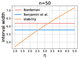
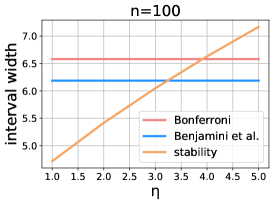
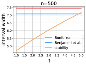
The proof of validity of this construction relies on our notion of stability, introduced in later sections; we defer the analysis of Claim 1 to the Supplement. Note that, as η𝜂\eta and δ𝛿\delta decrease toward zero, the noise level increases and the intervals approach classical, non-selective intervals. In general, η𝜂\eta is the key parameter that trades off the information used for selection versus inference: small η𝜂\eta corresponds to using more information for inference, while large η𝜂\eta corresponds to prioritizing selection quality. Figure 1 illustrates how the interval width changes with η𝜂\eta, in comparison to baselines, for σ=1,δ=0.5formulae-sequence𝜎1𝛿0.5\sigma=1,\delta=0.5, and varying n𝑛n.

Refer to captionRefer to captionRefer to caption

Figure 1: Confidence interval width around the “winning” effect, computed via the Bonferroni correction, Benjamini et al. [8] correction, and our stability-based approach. From left to right, we increase the value of n{50,100,500}𝑛50100500n\in\{50,100,500\} and keep σ=1𝜎1\sigma=1 fixed.

Note that if there is significant separation between μisubscript𝜇subscript𝑖\mu_{i_{*}} and the other effects, i^subscript^𝑖\hat{i}_{*} will likely be equal to isubscript𝑖i_{*} even for small η𝜂\eta. If, on the other hand, there are multiple effects of similar magnitude, the randomization will smooth out the selection and place non-negligible probability on all the competitive effects. In particular, to ensure i^=isubscript^𝑖subscript𝑖\hat{i}_{*}=i_{*} with high probability, it suffices to have η𝜂\eta inversely proportional to the gap between the largest and second largest observed effect, Δ=yimaxjiyjΔsubscript𝑦subscript𝑖subscript𝑗subscript𝑖subscript𝑦𝑗\Delta=y_{i_{*}}-\max_{j\neq i_{*}}y_{j}.

Claim 2.

If η4log(n/(2δ))z1αδ/(2n)Δ𝜂4𝑛2superscript𝛿subscript𝑧1𝛼𝛿2𝑛Δ\eta\geq\frac{4\log(n/(2\delta^{\prime}))z_{1-\alpha\delta/(2n)}}{\Delta} for some δ(0,1)superscript𝛿01\delta^{\prime}\in(0,1), then i^=isubscript^𝑖subscript𝑖\hat{i}_{*}=i_{*} with probability at least 1δ1superscript𝛿1-\delta^{\prime} over the randomness in the selection.
As a result, for large enough ΔΔ\Delta, the approach of Claim 1 allows selecting isubscript𝑖i_{*} with high probability while providing a tighter correction than the baselines.

Vignette 2: Feature selection.

In the second example we look at inference after data-driven feature selection. Suppose we have a fixed design matrix, Xn×d𝑋superscript𝑛𝑑X\in\mathbb{R}^{n\times d}, with n𝑛n observations and d𝑑d features and a corresponding outcome vector y𝒩(μ,σ2I)nsimilar-to𝑦𝒩𝜇superscript𝜎2𝐼superscript𝑛y\sim\mathcal{N}(\mu,\sigma^{2}I)\in\mathbb{R}^{n}. Denote by Xisubscript𝑋𝑖X_{i} the columns of X𝑋X, for i[d]𝑖delimited-[]𝑑i\in[d]. We would like to select a model corresponding to a subset of the d𝑑d features, and perform valid inference on the least-squares target after regressing y𝑦y on the selected features only. This problem is discussed in depth by Berk et al. [9].

We set this problem up more generally in later sections; to keep this illustration light, assume that the features are normalized so that Xi2=1subscriptnormsubscript𝑋𝑖21\|X_{i}\|_{2}=1 and we are selecting a single feature. Then, this problem amounts to doing inference on Xiμsuperscriptsubscript𝑋subscript𝑖top𝜇X_{i_{*}}^{\top}\mu, where isubscript𝑖i_{*} is the selected feature. Again, we note that this is a random inferential target since isubscript𝑖i_{*} is data-dependent.

Suppose that the goal of selection is to simply maximize the absolute correlation of the selected feature with y𝑦y: i=argmaxi|Xiy|subscript𝑖subscriptargmax𝑖superscriptsubscript𝑋𝑖top𝑦i_{*}=\operatorname*{arg\,max}_{i}|X_{i}^{\top}y|. Then, our results imply the following.

Claim 3.

Suppose that we select i^=argmaxi|Xiy+ξi|subscript^𝑖subscriptargmax𝑖superscriptsubscript𝑋𝑖top𝑦subscript𝜉𝑖\hat{i}_{*}=\operatorname*{arg\,max}_{i}|X_{i}^{\top}y+\xi_{i}|, where ξii.i.d.Lap(2z1αδ/(2d)η)\xi_{i}\stackrel{{\scriptstyle\mathrm{i.i.d.}}}{{\sim}}\mathrm{Lap}\left(\frac{2z_{1-\alpha\delta/(2d)}}{\eta}\right), for user-chosen parameters η>0,δ(0,1)formulae-sequence𝜂0𝛿01\eta>0,\delta\in(0,1). Then,

{Xi^μ(Xi^y±z1α(1δ)eη/2σ)}1α.superscriptsubscript𝑋subscript^𝑖top𝜇plus-or-minussuperscriptsubscript𝑋subscript^𝑖top𝑦subscript𝑧1𝛼1𝛿superscript𝑒𝜂2𝜎1𝛼\mathbb{P}\!\left\{{X_{\hat{i}_{*}}^{\top}\mu\in(X_{\hat{i}_{*}}^{\top}y\pm z_{1-\alpha(1-\delta)e^{-\eta}/2}\sigma)}\right\}\geq 1-\alpha.

Again, as η𝜂\eta and δ𝛿\delta tend toward zero, the intervals approach non-selective intervals, and the relationship between η𝜂\eta and the gap between the largest and second largest correlation, Δ=|Xiy|maxji|Xjy|Δsuperscriptsubscript𝑋subscript𝑖top𝑦subscript𝑗subscript𝑖superscriptsubscript𝑋𝑗top𝑦\Delta=|X_{i_{*}}^{\top}y|-\max_{j\neq i_{*}}|X_{j}^{\top}y|, drives the accuracy of selection.

Claim 4.

If η4log(d/(2δ))z1αδ/(2d)Δ𝜂4𝑑2superscript𝛿subscript𝑧1𝛼𝛿2𝑑Δ\eta\geq\frac{4\log(d/(2\delta^{\prime}))z_{1-\alpha\delta/(2d)}}{\Delta} for some δ(0,1)superscript𝛿01\delta^{\prime}\in(0,1), then i^=isubscript^𝑖subscript𝑖\hat{i}_{*}=i_{*} with probability at least 1δ1superscript𝛿1-\delta^{\prime} over the randomness in the selection.
Refer to captionRefer to captionRefer to caption

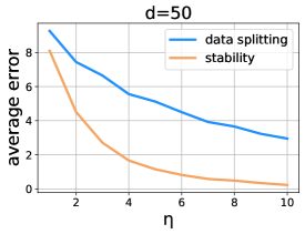
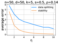
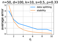
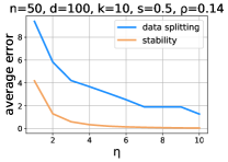
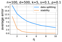
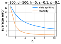
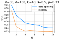
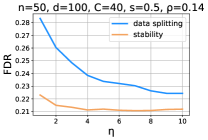
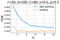
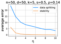
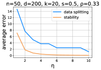
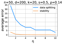
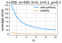
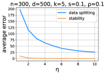
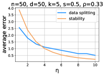
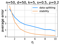
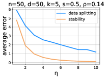
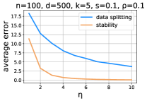
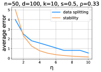
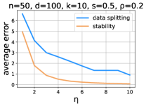
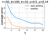
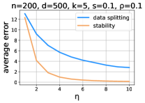
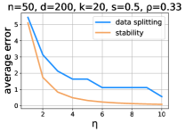
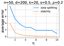
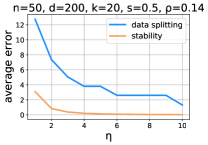
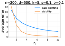
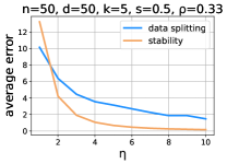
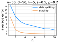
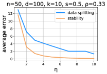
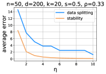
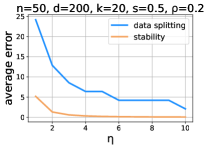
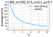
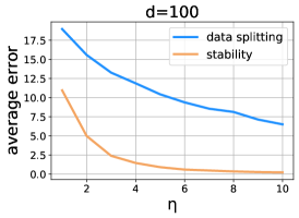
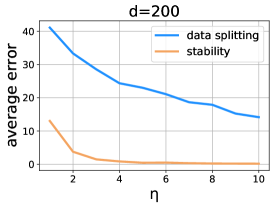
Figure 2: Average error, defined as maxi|Xiy||Xi^y|subscript𝑖superscriptsubscript𝑋𝑖top𝑦superscriptsubscript𝑋subscript^𝑖top𝑦\max_{i}|X_{i}^{\top}y|-|X_{\hat{i}_{*}}^{\top}y|, achieved by data splitting and our stability-based approach. We use one of the experimental setups in Section 9. The rows of X𝑋X are drawn i.i.d. from an equicorrelated multivariate Gaussian distribution with pairwise correlation ρ=0.5𝜌0.5\rho=0.5. The outcome is generated as y=Xβ+ϵ𝑦𝑋𝛽italic-ϵy=X\beta+\epsilon, where ϵitalic-ϵ\epsilon is isotropic Gaussian noise and half of the entries in β𝛽\beta are zero and half are sampled independently from Exp(0.2)Exp0.2\mathrm{Exp}(0.2). From left to right, we increase the value of d{50,100,200}𝑑50100200d\in\{50,100,200\} and keep n=50𝑛50n=50 fixed.

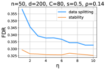
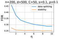
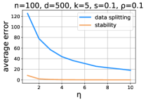
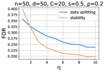
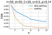
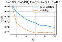
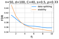
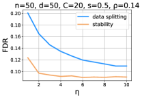
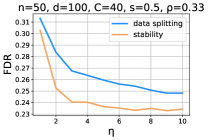
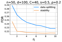
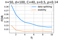
An alternative, equally simple solution to inference after feature selection is data splitting: we use a fraction f(0,1)𝑓01f\in(0,1) of the data for selection and the remaining 1f1𝑓1-f fraction for inference. In Section 5.1 we present a more detailed comparison with data splitting. For now we remark that, given that both data splitting and stability lead to intervals that look like classical intervals with an additional correction factor, every parameter η𝜂\eta has a corresponding parameter ff(η)𝑓𝑓𝜂f\equiv f(\eta) that yields data-splitting intervals of roughly the same width as stability-based intervals (given a fixed δ𝛿\delta such as 0.50.50.5). However, we observe that stability can be a significantly more powerful solution. Figure 2 compares the error of data splitting with the error of the stability solution described in Claim 3 in a simple simulation setting.

Finally, we emphasize that stability can be applied to the problem of feature selection even when data splitting is not an option, such as when there are spatial or temporal dependencies in the data.

3 Related work

In this section, we elaborate on the comparisons between our work and existing work in post-selection inference, and additionally discuss relevant work in the algorithmic stability literature.

Simultaneous coverage.

In the formulation of post-selection inference by Berk et al. [9], the goal is to construct simultaneous confidence intervals (as per Eq. (3)) that are valid for any model selection method M^:y:^𝑀𝑦\hat{M}:y\rightarrow\mathcal{M}, for a pre-specified model class \mathcal{M}. The framework of Berk et al. was subsequently generalized by Bachoc et al. [2] to handle distributions beyond the homoscedastic Gaussian, as initially assumed. These proposals are computationally infeasible in high dimensions as they essentially require looking for the “worst possible” model M𝑀M\in\mathcal{M}, one that implies the largest so-called PoSI (Post-Selection Inference) constant, an analog of which we introduce and characterize in the context of stability. More recent work has proposed computationally efficient confidence regions via UPoSI [32].

Another approach to valid post-selection inferences that applies to general selection rules is data splitting [42]: split the data into two disjoint subsets, then use one subset to select the inferential target and the other subset to perform inference. Data splitting is appealing because, if the two subsets of the data are independent, classical inferences will be valid regardless of the selection procedure. However, data splitting is not universally applicable as one cannot always obtain two independent data sets, and even if applicable, it can suffer a significant loss in power, such as when only a few samples capture some relevant information. Our stability-based approach does not rely on any independence assumption between different observations, and, as illustrated in Figure 2, it can be a more powerful solution than data splitting when the latter is applicable. We give a further discussion of data splitting and its relationship to stability in Section 5.1.

All the aforementioned strategies strive for robustness: they protect against all selection procedures. For specific selection procedures, however, the intervals computed by simultaneous methods and related approaches are unnecessarily wide, as they do not exploit any knowledge of how the analyst arrives at the selected target. Recent work aims to address this issue in the framework of simultaneous coverage over the selected variables (SoS) by constructing SoS-controlling confidence intervals for k𝑘k seemingly largest effects [8]. Our work likewise implies SoS intervals, by putting forward a general stability perspective and analyzing the relationship between stability and interval width for arbitrary stable procedures.

Conditional coverage.

Conditional methods [24] exploit properties of the selection procedure. However, they control a different error criterion than simultaneous methods. In particular, the goal of conditional post-selection inference is to design CISsubscriptCI𝑆\mathrm{CI}_{S} such that

{βSCIS|S^=S}1α,conditional-setsubscript𝛽𝑆subscriptCI𝑆^𝑆𝑆1𝛼\mathbb{P}\!\left\{{\beta_{S}\in\mathrm{CI}_{S}}\ \middle|\ {\hat{S}=S}\right\}\geq 1-\alpha,

for all fixed selections S𝑆S.

For a fixed selection procedure, conditional post-selection inference aims to characterize the distribution of the data given S^=S^𝑆𝑆\hat{S}=S, and then using the knowledge of this conditional distribution it computes CISsubscriptCI𝑆\mathrm{CI}_{S}. This approach is tailored to the selection method at hand, and existing work has derived intervals for model selection via methods such as the LASSO [35], marginal screening, orthogonal matching pursuit [34], forward stepwise, and LARS [56].

It is often remarked that the conditional approach leads to overconditioning, thus leading to wide intervals [29]. Informally, overconditioning refers to the phenomenon of overstating the cost of selection, thus leaving little information for inference. Surprisingly, it has even been observed that simultaneous approaches can in some cases yield smaller intervals, due to the intervals being unconditional rather than conditional [2]. One attempt at narrowing down the intervals involves choosing a better event on which to condition [37]. Another solution to overconditioning which is relevant to the present context is the idea of randomizing the selection procedure [52, 53, 54, 30, 40, 39, 10]. Notably, the pioneering work in this direction due to Tian and Taylor [52] proves a central limit theorem that asymptotically relates the validity of statistical inferences without selection to their selective counterparts, a result similar in flavor to our Theorem 2. However, existing randomization proposals suffer several drawbacks. One is that they give little insight into the tradeoff between confidence interval width and the loss in utility from the additional noise. Another issue is that inference is based on a selective pivot which, unlike in exact conditional approaches, lacks closed-form expressions. As a result, to approximate the pivot, existing work resorts to computationally expensive sampling [54, 52], which is generally infeasible in high dimensions. There are other, computationally-efficient approaches which aim to approximate the pivot [40, 39], although these are only approximate and the general theory applies to restricted classes of selection problems.

Although our primary goal is to provide unconditional guarantees, in Section 7 we will also discuss implications of stability for conditional inference.

We also point out the work of Andrews et al. [1], who propose a hybrid approach that interpolates between unconditional and conditional post-selection inference to obtain smaller confidence intervals relative to a purely conditional approach.

Algorithmic stability.

The technical tools of this paper are rooted in the theory of differential privacy [18, 17] and its extensions [20, 4]. Initially, differential privacy was developed as a standard for private data analysis. A more recent line of work, typically referred to as adaptive data analysis [see, e.g., 21, 20, 5], has recognized that a stability concept can be extracted from differential privacy and exploited to obtain perturbation-based generalization guarantees in learning theory. Superficially, adaptive data analysis has the same goal as post-selection inference—developing statistical tools for valid inference when hypotheses about the data are also data-driven—but the typical formalization of this problem is not directly comparable to that of the canonical post-selection inference setup in regression. The conceptual connection between the two areas has, however, been recognized (dating back to at least the seminal work of Tian and Taylor [52]), and several existing works discuss selective hypothesis tests and stability-based corrections to arbitrary selective p𝑝p-values [43, 45]. Our work does not aim to contribute to adaptive data analysis per se; rather, we build on and adapt existing tools in this literature for the purpose of providing post-selection corrections for common selection problems, such as within the framework put forward by Berk et al. [9]. Finally, we note that connections between stability and generalization are not new [11], and stability ideas have been utilized to construct predictive confidence intervals [47, 3].

4 Algorithmic stability and selection

The formal theory of algorithmic stability characterizes how the output of an algorithm changes when the input is perturbed. Randomized algorithms have as output a random variable; therefore, to study the stability of a randomized algorithm, an appropriate notion of closeness of two random variables is required. The particular notion of closeness considered in differential privacy and related work is known as indistinguishability, or max-divergence.

Definition 1 (Indistinguishability).

We say that a random variable Q𝑄Q is (η,τ)𝜂𝜏(\eta,\tau)-indistinguishable from W𝑊W, denoted Qη,τWsubscript𝜂𝜏𝑄𝑊Q\approx_{\eta,\tau}W, if for all measurable sets 𝒪𝒪\mathcal{O},

{Q𝒪}eη{W𝒪}+τ.𝑄𝒪superscript𝑒𝜂𝑊𝒪𝜏\mathbb{P}\!\left\{{Q\in\mathcal{O}}\right\}\leq e^{\eta}\mathbb{P}\!\left\{{W\in\mathcal{O}}\right\}+\tau.

Roughly speaking, τ𝜏\tau bounds the probability of the event that Q𝑄Q and W𝑊W are “very different.” For fixed τ[0,1]𝜏01\tau\in[0,1], the parameter η𝜂\eta is meant to capture how similar the distributions of Q𝑄Q and W𝑊W are—the larger η𝜂\eta is the larger the divergence between Q𝑄Q and W𝑊W can be. One should think of τ𝜏\tau as being at most a small factor proportional to the miscoverage probability α𝛼\alpha.

We now formally introduce the main notion of algorithmic stability considered in this paper. The algorithm whose stability we analyze will usually be a selection algorithm.

Definition 2 (Stability).

Let 𝒜:n𝒮:𝒜superscript𝑛𝒮\mathcal{A}:\mathbb{R}^{n}\rightarrow\mathcal{S} be a randomized algorithm. We say that 𝒜𝒜\mathcal{A} is (η,τ,ν)𝜂𝜏𝜈(\eta,\tau,\nu)-stable with respect to a distribution 𝒫𝒫\mathcal{P} supported on nsuperscript𝑛\mathbb{R}^{n} if there exists a random variable A0subscript𝐴0A_{0}, possibly dependent on 𝒫𝒫\mathcal{P}, such that

𝒫{ωn:𝒜(ω)η,τA0}1ν.𝒫conditional-set𝜔superscript𝑛subscript𝜂𝜏𝒜𝜔subscript𝐴01𝜈\mathcal{P}\left\{\omega\in\mathbb{R}^{n}:\mathcal{A}(\omega)\approx_{\eta,\tau}A_{0}\right\}\geq 1-\nu.

This notion is a special case of typical stability introduced by Bassily and Freund [4]. It is closely related to the notions of perfect generalization [15] and max-information [20]. Unless stated otherwise, whenever we use the term stability we will assume stability in the sense of Definition 2. The parameter ν𝜈\nu can in principle take on any value in [0,1]01[0,1] but in practice we will set it to be proportional to α𝛼\alpha.

We will only invoke stability with respect to the data distribution, which we will denote 𝒫ysubscript𝒫𝑦\mathcal{P}_{y}. Thus, for simplicity, when we say that 𝒜𝒜\mathcal{A} is (η,τ,ν)𝜂𝜏𝜈(\eta,\tau,\nu)-stable we are implicitly assuming that 𝒫ysubscript𝒫𝑦\mathcal{P}_{y} is the reference distribution.

Throughout we will use S^()^𝑆\hat{S}(\cdot) to denote a possibly randomized selection algorithm, which takes as input the data y𝑦y and outputs a selection that determines the inferential target. For example, S^^𝑆\hat{S} could be a model selection algorithm such as in the second vignette, or it could be an algorithm that selects an effect that is the focus of subsequent inference, such as in the first vignette. With a slight abuse of notation, we will use S^^𝑆\hat{S} to denote both the mapping from the data to the selection as well as the selection itself, S^(y)S^^𝑆𝑦^𝑆\hat{S}(y)\equiv\hat{S}.

Intuitively, S^^𝑆\hat{S} will be stable if we can “guess” the distribution of S^(y)^𝑆𝑦\hat{S}(y) (conditional on y𝑦y) with only knowledge of the data distribution 𝒫ysubscript𝒫𝑦\mathcal{P}_{y}, not the data y𝑦y itself.

Example 1.

To provide intuition for Definition 2, we present one simple mechanism for achieving stability. Although basic, this mechanism will be a fundamental building block in our stability proofs. Suppose that we wish to compute wysuperscript𝑤top𝑦w^{\top}y, for some fixed vector w𝑤w, and suppose that we take 𝒫ysubscript𝒫𝑦\mathcal{P}_{y} to be 𝒩(μ,σ2I)𝒩𝜇superscript𝜎2𝐼\mathcal{N}(\mu,\sigma^{2}I) with known σ>0𝜎0\sigma>0. Let 𝒜(y)=wy+ξ𝒜𝑦superscript𝑤top𝑦𝜉\mathcal{A}(y)=w^{\top}y+\xi, where ξLap(z1ν/2σw2η)similar-to𝜉Lapsubscript𝑧1𝜈2𝜎subscriptnorm𝑤2𝜂\xi\sim\text{Lap}\left(\frac{z_{1-\nu/2}\sigma\|w\|_{2}}{\eta}\right), for user-specified parameters η>0,ν(0,1)formulae-sequence𝜂0𝜈01\eta>0,\nu\in(0,1). Here, Lap(b)Lap𝑏\text{Lap}(b) denotes a draw from the zero-mean Laplace distribution with parameter b𝑏b, independent of y𝑦y. We argue that this mechanism is (η,0,ν)𝜂0𝜈(\eta,0,\nu)-stable. First, we know

{|wywμ|z1ν/2σw2}superscript𝑤top𝑦superscript𝑤top𝜇subscript𝑧1𝜈2𝜎subscriptnorm𝑤2\displaystyle\mathbb{P}\!\left\{{|w^{\top}y-w^{\top}\mu|\geq z_{1-\nu/2}\sigma\|w\|_{2}}\right\}
={|𝒩(0,σ2w22)|z1ν/2σw2}=ν.absent𝒩0superscript𝜎2superscriptsubscriptnorm𝑤22subscript𝑧1𝜈2𝜎subscriptnorm𝑤2𝜈\displaystyle=\mathbb{P}\!\left\{{|\mathcal{N}(0,\sigma^{2}\|w\|_{2}^{2})|\geq z_{1-\nu/2}\sigma\|w\|_{2}}\right\}=\nu.

Denote Yν={ωn:|wωwμ|z1ν/2σw2}subscript𝑌𝜈conditional-set𝜔superscript𝑛superscript𝑤top𝜔superscript𝑤top𝜇subscript𝑧1𝜈2𝜎subscriptnorm𝑤2Y_{\nu}=\{\omega\in\mathbb{R}^{n}:|w^{\top}\omega-w^{\top}\mu|\leq z_{1-\nu/2}\sigma\|w\|_{2}\}, and notice that we have shown that {yYν}=1ν𝑦subscript𝑌𝜈1𝜈\mathbb{P}\!\left\{{y\in Y_{\nu}}\right\}=1-\nu.

Now let A0=𝒜(μ)subscript𝐴0𝒜𝜇A_{0}=\mathcal{A}(\mu). Since the ratio of densities of ξLap(b)similar-to𝜉Lap𝑏\xi\sim\text{Lap}(b) and its shifted counterpart x+ξ𝑥𝜉x+\xi is upper bounded by e|x|/bsuperscript𝑒𝑥𝑏e^{|x|/b}, we can conclude that for all ωYν𝜔subscript𝑌𝜈\omega\in Y_{\nu} and measurable sets 𝒪𝒪\mathcal{O},

{𝒜(ω)𝒪}{𝒜(μ)𝒪}eη;𝒜𝜔𝒪𝒜𝜇𝒪superscript𝑒𝜂\frac{\mathbb{P}\!\left\{{\mathcal{A}(\omega)\in\mathcal{O}}\right\}}{\mathbb{P}\!\left\{{\mathcal{A}(\mu)\in\mathcal{O}}\right\}}\leq e^{\eta};

that is, we have 𝒜(ω)η,0A0subscript𝜂0𝒜𝜔subscript𝐴0\mathcal{A}(\omega)\approx_{\eta,0}A_{0} for all ωYν𝜔subscript𝑌𝜈\omega\in Y_{\nu}. Putting everything together, we see that 𝒜()𝒜\mathcal{A}(\cdot) is (η,0,ν)𝜂0𝜈(\eta,0,\nu)-stable with respect to 𝒫ysubscript𝒫𝑦\mathcal{P}_{y}.

5 Confidence intervals after stable selection

Given the assumption of (η,τ,ν)𝜂𝜏𝜈(\eta,\tau,\nu)-stability, we now show how a simple modification to classical confidence intervals suffices to correct for selective inferences. This correction is valid regardless of any additional property of the selection criterion.

The main intuition behind this assertion is the following. If the selection algorithm is stable, then by Definition 2 there must exist an oracle selection S^0subscript^𝑆0\hat{S}_{0} such that S^(y)^𝑆𝑦\hat{S}(y) and S^0subscript^𝑆0\hat{S}_{0} are indistinguishable. Note that S^0subscript^𝑆0\hat{S}_{0} is independent of y𝑦y. Since S^0subscript^𝑆0\hat{S}_{0} is indistinguishable from S^(y)^𝑆𝑦\hat{S}(y), we can pretend that S^0subscript^𝑆0\hat{S}_{0} is the selection of interest. Furthermore, since S^0subscript^𝑆0\hat{S}_{0} and y𝑦y are independent, we are free to use y𝑦y for inference. Stability ensures that, despite data reuse, inference behaves almost like with data splitting, in which we perform selection on one batch of data and then use independent data for constructing intervals.

We state a technical lemma, similar to Lemma 3.3 by Bassily and Freund [4], that we use to prove our main theorem. We include a proof of Lemma 1 in the Supplement.

Lemma 1.

Let S^:n𝒮:^𝑆superscript𝑛𝒮\hat{S}:\mathbb{R}^{n}\rightarrow\mathcal{S} be an (η,τ,ν)𝜂𝜏𝜈(\eta,\tau,\nu)-stable selection algorithm and let S^0subscript^𝑆0\hat{S}_{0} be the corresponding oracle selection. Then, it holds that

(y,S^(y))η,τ+ν(y,S^0).subscript𝜂𝜏𝜈𝑦^𝑆𝑦𝑦subscript^𝑆0(y,\hat{S}(y))\approx_{\eta,\tau+\nu}(y,\hat{S}_{0}). (1)

Equipped with Lemma 1, we can now describe how to construct post-selection-valid confidence intervals after stable selection.

Suppose that, under selection S𝑆S, our target of inference is βSsubscript𝛽𝑆\beta_{S}. Moreover, suppose that CIS(α)superscriptsubscriptCI𝑆𝛼\mathrm{CI}_{S}^{(\alpha)} are valid confidence intervals at level 1α1𝛼1-\alpha for any fixed S𝑆S, meaning that

{βSCIS(α)}α.subscript𝛽𝑆superscriptsubscriptCI𝑆𝛼𝛼\mathbb{P}\!\left\{{\beta_{S}\not\in\mathrm{CI}_{S}^{(\alpha)}}\right\}\leq\alpha.

Such intervals are provided by classical theory.

Theorem 2 formally states how to construct confidence intervals for an adaptive target βS^subscript𝛽^𝑆\beta_{\hat{S}}, when S^^𝑆\hat{S} is selected in a stable way. This is the key result of our paper.

Theorem 2.

Fix δ(0,1)𝛿01\delta\in(0,1), and let S^^𝑆\hat{S} be an (η,τ,ν)𝜂𝜏𝜈(\eta,\tau,\nu)-stable selection algorithm. Then,

{βS^CIS^(δeη)}δ+τ+ν.subscript𝛽^𝑆superscriptsubscriptCI^𝑆𝛿superscript𝑒𝜂𝛿𝜏𝜈\mathbb{P}\!\left\{{\beta_{\hat{S}}\not\in\mathrm{CI}_{\hat{S}}^{(\delta e^{-\eta})}}\right\}\leq\delta+\tau+\nu.

In words, if S^^𝑆\hat{S} is (η,τ,ν)𝜂𝜏𝜈(\eta,\tau,\nu)-stable, we can pretend that there is no selection bias and simply construct classical intervals, albeit at a more conservative level, to achieve validity. If we set the target error level to be δeη𝛿superscript𝑒𝜂\delta e^{-\eta}, then the realized error level will be at most δ+τ+ν𝛿𝜏𝜈\delta+\tau+\nu. For example, if we let τ=ν=α/3𝜏𝜈𝛼3\tau=\nu=\alpha/3, then to get coverage at level 1α1𝛼1-\alpha we can set the target coverage level to be α/3eη𝛼3superscript𝑒𝜂\alpha/3\cdot e^{-\eta}.

5.1 Comparison with data splitting

In many scenarios it is possible to split the data into two independent chunks, one to be used for selection and the other to be reserved for inference. Classical inferences are then valid because the inferential target is determined before seeing any of the data used in the inference step. This simple baseline for valid inference after selection is called data splitting. In this section, we illuminate the relationship between our approach via stability and data splitting.

First we want to emphasize that the stability principle is applicable even with dependent samples: Theorem 2 can be applied even when it is not clear how to create two independent subsets of the data. Moreover, in some selection problems data splitting makes little conceptual sense, such as in our first motivating vignette about inference on the winning effect.

The appeal of data splitting lies in its broad applicability. As long as the data can be split into two independent components, the criteria for choosing the inferential target can be arbitrary. Therefore, data splitting provides a selection-agnostic correction, universally valid across all possible selection strategies.

Conceptually, stability lies somewhere between data splitting and conditional post-selection inference. It computes a correction level as a function of how adaptive the selection is to the data, thereby adapting to some properties of the selection rule like conditional inference methods. However, at the same time it provides a correction that is universally valid across all possible selection strategies with the same level of stability, which can be seen as a refinement of the principle of data splitting.

To illustrate the conceptual difference between the stability principle and the data splitting principle, suppose that in the latter case we allocate f𝑓f-fraction of the data to selection, and (1f)1𝑓(1-f)-fraction to inference. Then, the resulting intervals will roughly look like classical intervals augmented by a factor of 11f11𝑓\sqrt{\frac{1}{1-f}} regardless of how the selection is performed.

In contrast, the stability approach augments classical intervals as a function of the adaptivity of the selection algorithm. Suppose for concreteness that y𝒩(μ,I)similar-to𝑦𝒩𝜇𝐼y\sim\mathcal{N}(\mu,I) and we are considering doing inference on one of two targets, v0μsuperscriptsubscript𝑣0top𝜇v_{0}^{\top}\mu or v1μsuperscriptsubscript𝑣1top𝜇v_{1}^{\top}\mu, where the selection S^{0,1}^𝑆01\hat{S}\in\{0,1\} depends on the data y𝑦y. Consider three different selection methods:

  • S^=1^𝑆1\hat{S}=1 no matter what the data vector is.

  • S^=1^𝑆1\hat{S}=1 if y¯:=1ni=1nyi0assign¯𝑦1𝑛superscriptsubscript𝑖1𝑛subscript𝑦𝑖0\bar{y}:=\frac{1}{n}\sum_{i=1}^{n}y_{i}\geq 0, and S^=0^𝑆0\hat{S}=0 otherwise.

  • S^=1^𝑆1\hat{S}=1 if X1y0superscriptsubscript𝑋1top𝑦0X_{1}^{\top}y\geq 0 for some unit vector X1subscript𝑋1X_{1}, and S^=0^𝑆0\hat{S}=0 otherwise.

We can write all three procedures as S^=𝟏{wy0}^𝑆1superscript𝑤top𝑦0\hat{S}=\mathbf{1}\{w^{\top}y\geq 0\}; in the first case w=0𝑤0w=0, in the second case w=1n𝟏𝑤1𝑛1w=\frac{1}{n}\mathbf{1}, and in the third case w=X1𝑤subscript𝑋1w=X_{1}.

Let us fix the noise level γ>0𝛾0\gamma>0 and select S^=𝟏{wy+ξ0}^𝑆1superscript𝑤top𝑦𝜉0\hat{S}=\mathbf{1}\{w^{\top}y+\xi\geq 0\}, where ξLap(γ)similar-to𝜉Lap𝛾\xi\sim\text{Lap}(\gamma). The first method is trivially (0,0,0)000(0,0,0)-stable for any level γ𝛾\gamma, hence we can simply use y𝑦y for inference without any correction. Based on the same analysis as in the example in Section 4, the second selection method is (2log(2/ν)/(γn),0,ν)22𝜈𝛾𝑛0𝜈(\sqrt{2\log(2/\nu)}/(\gamma\sqrt{n}),0,\nu)-stable for all ν> 0𝜈 0\nu>\leavevmode\nobreak\ 0; i.e., it is (2log(4/α)/(γn),0,α/2)24𝛼𝛾𝑛0𝛼2(\sqrt{2\log(4/\alpha)}/(\gamma\sqrt{n}),0,\alpha/2)-stable. Similarly, the third selection method is (2log(4/α)/γ,0,α/2)24𝛼𝛾0𝛼2(\sqrt{2\log(4/\alpha)}/\gamma,0,\alpha/2)-stable.

We can thus observe that, even though in all three examples we perturb the selection by the same constant level of noise, the stability approach exploits the fact that some selection criteria are more stable than others and this is reflected in the resulting stability parameter. By Theorem 2, this stability parameter, in turn, directly determines the correction factor, i.e., how conservative we need to make classical inferences for them to be valid post selection.

While data splitting and stability come with conceptual differences, they also have technical similarities. In particular, each one has a leading parameter—f(0,1)𝑓01f\in(0,1) in the case of data splitting and η>0𝜂0\eta>0 in the case of stability—and this parameter interpolates between two extremes. One extreme is when all information is reserved for inference (attained when f=0𝑓0f=0 and η=0𝜂0\eta=0 respectively) and the other is when all information is used for selection (attained when f=1𝑓1f=1 and η𝜂\eta\rightarrow\infty respectively). Therefore, it might make sense to ask how the two interpolations relate.

For every η𝜂\eta, there is an f(η)𝑓𝜂f(\eta) such that, if we used f(η)𝑓𝜂f(\eta)-fraction of the data for selection and 1f(η)1𝑓𝜂1-f(\eta) for inference, we would approximately get the same interval correction. We sketch the derivation of f(η)𝑓𝜂f(\eta) in the case of normal intervals for simplicity, however this calculation can be generalized to other distributions. We will assume that ν+τδα𝜈𝜏𝛿𝛼\nu+\tau\leq\delta\alpha for some δ(0,1)𝛿01\delta\in(0,1); then, the intervals resulting from (η,τ,ν)𝜂𝜏𝜈(\eta,\tau,\nu)-stability are of width proportional to z1(1δ)α2eη.subscript𝑧11𝛿𝛼2superscript𝑒𝜂z_{1-(1-\delta)\frac{\alpha}{2}e^{-\eta}}. The intervals resulting from data splitting are of width proportional to z1α2(1f(η))1/2.subscript𝑧1𝛼2superscript1𝑓𝜂12z_{1-\frac{\alpha}{2}}(1-f(\eta))^{-1/2}. By equating the two expressions to achieve the same width and simplifying, we obtain

f(η)=1(z1α2z1(1δ)α2eη)2log11δ+ηlog2(1δ)α+η,𝑓𝜂1superscriptsubscript𝑧1𝛼2subscript𝑧11𝛿𝛼2superscript𝑒𝜂211𝛿𝜂21𝛿𝛼𝜂f(\eta)=1-\left(\frac{z_{1-\frac{\alpha}{2}}}{z_{1-(1-\delta)\frac{\alpha}{2}e^{-\eta}}}\right)^{2}\approx\frac{\log\frac{1}{1-\delta}+\eta}{\log\frac{2}{(1-\delta)\alpha}+\eta}, (2)

where the approximation on the right-hand side follows by a subgaussian approximation.

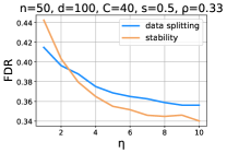
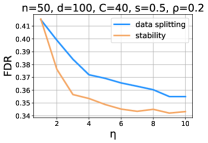
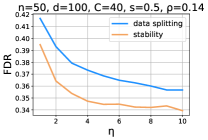
Of course, this sketch only gives intuition for when data splitting and stability imply equally powerful inference; it does not say anything about which selection is more accurate—one where we select on f(η)𝑓𝜂f(\eta)-fraction of the data, or one where we select on the whole data set in an η𝜂\eta-stable way. We will tackle this question empirically, as the notion of “more accurate” varies greatly depending on the context. In Figure 2 we used the splitting fraction in Eq. (2) and observed that stability outperforms data splitting. We provide further empirical comparisons in Section 9.

Finally, we mention another proposal that is conceptually closely related to data splitting, namely the (U,V)𝑈𝑉(U,V) decomposition of Rasines and Young [41]. Like stability, the (U,V)𝑈𝑉(U,V) decomposition allows the statistician to see all data points—more precisely, noisy versions thereof—both in the selection step and in the inference step. This is an important advantage over data splitting when there are only a few samples that capture information about certain directions. In contrast with stability, performing the (U,V)𝑈𝑉(U,V) decomposition does not rely on any properties of the selection method. However, finite-sample guarantees of this approach crucially rely on the data being Gaussian with known covariance, while the stability principle is applicable beyond Gaussianity and is robust to only having an estimate of the covariance.

6 Model selection in linear regression

In this section, we discuss an application of our stability tools to the problem of model selection in linear regression. We focus on the framework presented in the seminal work of Berk et al. [9]. We begin by reviewing the model and introduce the necessary notation.

Let Xn×d𝑋superscript𝑛𝑑X\in\mathbb{R}^{n\times d} denote a fixed design matrix, and let Xinsubscript𝑋𝑖superscript𝑛X_{i}\in\mathbb{R}^{n} denote the i𝑖i-th column of X𝑋X, for i[d]𝑖delimited-[]𝑑i\in[d]. We refer to vectors Xisubscript𝑋𝑖X_{i} as variables or features. For a subset M[d]𝑀delimited-[]𝑑M\subseteq[d], we denote by XMn×|M|subscript𝑋𝑀superscript𝑛𝑀X_{M}\in\mathbb{R}^{n\times|M|} the submatrix of X𝑋X given by selecting the columns indexed by M𝑀M. We make no assumptions about how n𝑛n and d𝑑d relate; in particular, we could have dnmuch-greater-than𝑑𝑛d\gg n.

By yn𝑦superscript𝑛y\in\mathbb{R}^{n} we denote the random vector of outcomes corresponding to X𝑋X. Importantly, we do not assume knowledge of a true data-generating process; for example, we do not assume that μ:=𝔼[y]assign𝜇𝔼delimited-[]𝑦\mu:=\mathbb{E}[y] can be expressed as a linear combination of {Xi}i=1dsuperscriptsubscriptsubscript𝑋𝑖𝑖1𝑑\{X_{i}\}_{i=1}^{d}. The vector μn𝜇superscript𝑛\mu\in\mathbb{R}^{n} is unconstrained and need not reside in the column space of X𝑋X. Rather, different subsets of {Xi}i=1dsuperscriptsubscriptsubscript𝑋𝑖𝑖1𝑑\{X_{i}\}_{i=1}^{d} provide different approximations to μ𝜇\mu, some better than others.

The statistician wishes to let the data decide how the initial pool of features should be reduced to a smaller set of seemingly relevant features, and then run linear regression on this smaller set. That is, the statistician chooses a set M^[d]^𝑀delimited-[]𝑑\hat{M}\subseteq[d] by running a model selection method on X,y𝑋𝑦X,y, and then aims to approximate yXM^β^M^𝑦subscript𝑋^𝑀subscript^𝛽^𝑀y\approx X_{\hat{M}}\hat{\beta}_{\hat{M}}, for some β^M^subscript^𝛽^𝑀\hat{\beta}_{\hat{M}}. As before, we will employ a conventional abuse of notation by letting M^M^(y)^𝑀^𝑀𝑦\hat{M}\equiv\hat{M}(y).

Assuming XM^subscript𝑋^𝑀X_{\hat{M}} has full column rank almost surely, the unique least-squares estimate in model M^^𝑀\hat{M} is given by

β^M^:=argminβ|M^|yXM^β22=(XM^XM^)1XM^y:=XM^+y,assignsubscript^𝛽^𝑀subscriptargmin𝛽superscript^𝑀superscriptsubscriptnorm𝑦subscript𝑋^𝑀𝛽22superscriptsuperscriptsubscript𝑋^𝑀topsubscript𝑋^𝑀1superscriptsubscript𝑋^𝑀top𝑦assignsuperscriptsubscript𝑋^𝑀𝑦\hat{\beta}_{\hat{M}}:=\operatorname*{arg\,min}_{\beta\in\mathbb{R}^{|\hat{M}|}}\|y-X_{\hat{M}}\beta\|_{2}^{2}=(X_{\hat{M}}^{\top}X_{\hat{M}})^{-1}X_{\hat{M}}^{\top}y:=X_{\hat{M}}^{+}y,

where we define XM^+:=(XM^XM^)1XM^assignsuperscriptsubscript𝑋^𝑀superscriptsuperscriptsubscript𝑋^𝑀topsubscript𝑋^𝑀1superscriptsubscript𝑋^𝑀topX_{\hat{M}}^{+}:=(X_{\hat{M}}^{\top}X_{\hat{M}})^{-1}X_{\hat{M}}^{\top} to be the pseudoinverse of XM^subscript𝑋^𝑀X_{\hat{M}}. For a fixed model M𝑀M, the target estimand of β^Msubscript^𝛽𝑀\hat{\beta}_{M} is

βM:=argminβ|M|𝔼[yXMβ22]=XM+μ,assignsubscript𝛽𝑀subscriptargmin𝛽superscript𝑀𝔼delimited-[]superscriptsubscriptnorm𝑦subscript𝑋𝑀𝛽22superscriptsubscript𝑋𝑀𝜇\beta_{M}:=\operatorname*{arg\,min}_{\beta\in\mathbb{R}^{|M|}}\mathbb{E}\left[\|y-X_{M}\beta\|_{2}^{2}\right]=X_{M}^{+}\mu,

and hence for a random model M^^𝑀\hat{M}, this implies a random target βM^=XM^+μsubscript𝛽^𝑀superscriptsubscript𝑋^𝑀𝜇\beta_{\hat{M}}=X_{\hat{M}}^{+}\mu.

We denote by βjMsubscript𝛽𝑗𝑀\beta_{j\cdot M} the entry of βMsubscript𝛽𝑀\beta_{M} corresponding to feature Xjsubscript𝑋𝑗X_{j}, for all jM𝑗𝑀j\in M. Note that βjMsubscript𝛽𝑗𝑀\beta_{j\cdot M} is not defined for jM𝑗𝑀j\not\in M. We adopt similar notation for the entries of β^Msubscript^𝛽𝑀\hat{\beta}_{M}.

Our goal is to construct simultaneous confidence intervals for the target of inference βM^subscript𝛽^𝑀\beta_{\hat{M}}. More precisely, we wish to design CIjM^(α)superscriptsubscriptCI𝑗^𝑀𝛼\mathrm{CI}_{j\cdot\hat{M}}^{(\alpha)} such that

{βjM^CIjM^(α),jM^}1α,formulae-sequencesubscript𝛽𝑗^𝑀superscriptsubscriptCI𝑗^𝑀𝛼for-all𝑗^𝑀1𝛼\mathbb{P}\!\left\{{\beta_{j\cdot\hat{M}}\in\mathrm{CI}_{j\cdot\hat{M}}^{(\alpha)},\leavevmode\nobreak\ \forall j\in\hat{M}}\right\}\geq 1-\alpha, (3)

for a fixed α(0,1)𝛼01\alpha\in(0,1) and a fixed selection procedure M^^𝑀\hat{M}. Note that the work of Berk et al. and various extensions [9, 2, 32] provide simultaneity both over the selected variables and over all selection methods, while we keep the selection method fixed. Our guarantees are simultaneous over the selected [cf. 8].

The confidence intervals resulting from our approach take the usual form,

CIjM^(K):=(β^jM^±Kσ^jM^),assignsubscriptCI𝑗^𝑀𝐾plus-or-minussubscript^𝛽𝑗^𝑀𝐾subscript^𝜎𝑗^𝑀\mathrm{CI}_{j\cdot\hat{M}}(K):=\left(\hat{\beta}_{j\cdot\hat{M}}\pm K\hat{\sigma}_{j\cdot\hat{M}}\right),

where σ^jM^2superscriptsubscript^𝜎𝑗^𝑀2\hat{\sigma}_{j\cdot\hat{M}}^{2} is an estimator of variance for the OLS estimate β^jM^subscript^𝛽𝑗^𝑀\hat{\beta}_{j\cdot\hat{M}}; e.g., the “sandwich” variance estimator [12]. Our goal is to find a suitable value of K𝐾K such that CIjM^(K)subscriptCI𝑗^𝑀𝐾\mathrm{CI}_{j\cdot\hat{M}}(K) are valid (1α)1𝛼(1-\alpha)-confidence intervals, as per Eq. (3). By analogy with Berk et al. [9], we refer to the minimal such valid K𝐾K as the PoSI constant. It is important to remember that, unlike in Berk et al., our PoSI constant depends on the selection procedure, rather than a family of all possible models.

The PoSI constant is well characterized when the model is fixed rather than determined in a data-driven fashion. For a fixed model M𝑀M and given α(0,1)𝛼01\alpha\in(0,1), we define KM,αsubscript𝐾𝑀𝛼K_{M,\alpha} to be the minimum value of K𝐾K such that

{maxjM|β^jMβjMσ^jM|K}α.subscript𝑗𝑀subscript^𝛽𝑗𝑀subscript𝛽𝑗𝑀subscript^𝜎𝑗𝑀𝐾𝛼\mathbb{P}\!\left\{{\max_{j\in M}\left|\frac{\hat{\beta}_{j\cdot M}-\beta_{j\cdot M}}{\hat{\sigma}_{j\cdot M}}\right|\geq K}\right\}\leq\alpha.

In other words, KM,αsubscript𝐾𝑀𝛼K_{M,\alpha} defines the PoSI constant when the model M𝑀M is specified up front and does not depend on the data; in this case, CIjM(KM,α)subscriptCI𝑗𝑀subscript𝐾𝑀𝛼\mathrm{CI}_{j\cdot M}(K_{M,\alpha}) are valid simultaneous intervals at level 1α1𝛼1-\alpha. For example, when y𝒩(μ,σ2I)similar-to𝑦𝒩𝜇superscript𝜎2𝐼y\sim\mathcal{N}(\mu,\sigma^{2}I), one simple way of providing a valid upper bound on KM,αsubscript𝐾𝑀𝛼K_{M,\alpha} is via standard z-scores or t-scores, after doing a Bonferroni correction over jM𝑗𝑀j\in M. Sharper estimates of KM,αsubscript𝐾𝑀𝛼K_{M,\alpha} can be obtained by exploiting the correlations between the regression coefficients to estimate the maximum z-score or t-score. Even in a distribution-free setting, it is common to determine KM,αsubscript𝐾𝑀𝛼K_{M,\alpha} via normal approximation [42, 33].

We are now ready to state a corollary of Theorem 2 that focuses on the problem of model selection in linear regression.

Corollary 1.

Fix δ(0,1)𝛿01\delta\in(0,1). Let M^^𝑀\hat{M} be an (η,τ,ν)𝜂𝜏𝜈(\eta,\tau,\nu)-stable model selection algorithm. For all jM^𝑗^𝑀j\in\hat{M}, let:

CIjM^(KM^,δeη)=(β^jM^±KM^,δeησ^jM^).subscriptCI𝑗^𝑀subscript𝐾^𝑀𝛿superscript𝑒𝜂plus-or-minussubscript^𝛽𝑗^𝑀subscript𝐾^𝑀𝛿superscript𝑒𝜂subscript^𝜎𝑗^𝑀\mathrm{CI}_{j\cdot\hat{M}}(K_{\hat{M},\delta e^{-\eta}})=\left(\hat{\beta}_{j\cdot\hat{M}}\pm K_{\hat{M},\delta e^{-\eta}}\hat{\sigma}_{j\cdot\hat{M}}\right).

Then,

{jM^:βjM^CIjM^(KM^,δeη)}δ+τ+ν.conditional-set𝑗^𝑀subscript𝛽𝑗^𝑀subscriptCI𝑗^𝑀subscript𝐾^𝑀𝛿superscript𝑒𝜂𝛿𝜏𝜈\mathbb{P}\!\left\{{\exists j\in\hat{M}:\beta_{j\cdot\hat{M}}\not\in\mathrm{CI}_{j\cdot\hat{M}}\left(K_{\hat{M},\delta e^{-\eta}}\right)}\right\}\leq\delta+\tau+\nu.

To provide further intuition, we instantiate Corollary 1 in the canonical setting of Gaussian observations. Let y𝒩(μ,σ2I)similar-to𝑦𝒩𝜇superscript𝜎2𝐼y\sim\mathcal{N}(\mu,\sigma^{2}I). If σ>0𝜎0\sigma>0 is known, we let σ^jM=σ((XMXM)1)jjsubscript^𝜎𝑗𝑀𝜎subscriptsuperscriptsuperscriptsubscript𝑋𝑀topsubscript𝑋𝑀1𝑗𝑗\hat{\sigma}_{j\cdot M}=\sigma\sqrt{((X_{M}^{\top}X_{M})^{-1})_{jj}}; otherwise, we assume we have access to an estimate of σ𝜎\sigma, denoted σ^^𝜎\hat{\sigma}, and let σ^jM=σ^((XMXM)1)jjsubscript^𝜎𝑗𝑀^𝜎subscriptsuperscriptsuperscriptsubscript𝑋𝑀topsubscript𝑋𝑀1𝑗𝑗\hat{\sigma}_{j\cdot M}=\hat{\sigma}\sqrt{((X_{M}^{\top}X_{M})^{-1})_{jj}}. Following the treatment of Berk et al. [9], we assume that σ^2σ2χr2rsimilar-tosuperscript^𝜎2superscript𝜎2superscriptsubscript𝜒𝑟2𝑟\hat{\sigma}^{2}\sim\sigma^{2}\frac{\chi_{r}^{2}}{r} for r𝑟r degrees of freedom and assume that σ^2β^jMperpendicular-tosuperscript^𝜎2subscript^𝛽𝑗𝑀\hat{\sigma}^{2}\perp\hat{\beta}_{j\cdot M} for all possible OLS estimates β^jMsubscript^𝛽𝑗𝑀\hat{\beta}_{j\cdot M}. If the full model is assumed to be correct, that is y𝒩(Xβ,σ2I)similar-to𝑦𝒩𝑋𝛽superscript𝜎2𝐼y\sim\mathcal{N}(X\beta,\sigma^{2}I), and n>d𝑛𝑑n>d, then this assumption is satisfied for r=nd𝑟𝑛𝑑r=n-d by setting σ^2=yXβ^22/(nd)superscript^𝜎2superscriptsubscriptnorm𝑦𝑋^𝛽22𝑛𝑑\hat{\sigma}^{2}=\|y-X\hat{\beta}\|_{2}^{2}/(n-d), where β^^𝛽\hat{\beta} is the OLS estimate in the full model. Even if the full model is not correct, there exist other ways of producing such a valid estimate of σ𝜎\sigma; we refer the reader to Berk et al. [9] for further discussion.

We denote by z1αsubscript𝑧1𝛼z_{1-\alpha} the 1α1𝛼1-\alpha quantile of the standard normal distribution, and by tr,1αsubscript𝑡𝑟1𝛼t_{r,1-\alpha} the 1α1𝛼1-\alpha quantile of the t𝑡t-distribution with r𝑟r degrees of freedom.

Corollary 2.

Fix δ(0,1)𝛿01\delta\in(0,1), and suppose y𝒩(μ,σ2I)similar-to𝑦𝒩𝜇superscript𝜎2𝐼y\sim\mathcal{N}(\mu,\sigma^{2}I). Further, let M^^𝑀\hat{M} be an (η,τ,ν)𝜂𝜏𝜈(\eta,\tau,\nu)-stable model selection algorithm. If σ𝜎\sigma is known, let:

CIjM^=(β^jM^±z1δ/(2|M^|eη)σ((XM^XM^)1)jj).subscriptCI𝑗^𝑀plus-or-minussubscript^𝛽𝑗^𝑀subscript𝑧1𝛿2^𝑀superscript𝑒𝜂𝜎subscriptsuperscriptsuperscriptsubscript𝑋^𝑀topsubscript𝑋^𝑀1𝑗𝑗\mathrm{CI}_{j\cdot\hat{M}}=\left(\hat{\beta}_{j\cdot\hat{M}}\pm z_{1-\delta/(2|\hat{M}|e^{\eta})}\sigma\sqrt{((X_{\hat{M}}^{\top}X_{\hat{M}})^{-1})_{jj}}\right).

If, on the other hand, σ𝜎\sigma is not known but there exists an estimate, σ^2σ2χr2rsimilar-tosuperscript^𝜎2superscript𝜎2superscriptsubscript𝜒𝑟2𝑟\hat{\sigma}^{2}\sim\sigma^{2}\frac{\chi_{r}^{2}}{r}, independent of the OLS estimates, let:

CIjM^=(β^jM^±tr,1δ/(2|M^|eη)σ^((XM^XM^)1)jj).subscriptCI𝑗^𝑀plus-or-minussubscript^𝛽𝑗^𝑀subscript𝑡𝑟1𝛿2^𝑀superscript𝑒𝜂^𝜎subscriptsuperscriptsuperscriptsubscript𝑋^𝑀topsubscript𝑋^𝑀1𝑗𝑗\mathrm{CI}_{j\cdot\hat{M}}=\left(\hat{\beta}_{j\cdot\hat{M}}\pm t_{r,1-\delta/(2|\hat{M}|e^{\eta})}\hat{\sigma}\sqrt{((X_{\hat{M}}^{\top}X_{\hat{M}})^{-1})_{jj}}\right).

In either case, we have

{jM^:βjM^CIjM^}δ+τ+ν.conditional-set𝑗^𝑀subscript𝛽𝑗^𝑀subscriptCI𝑗^𝑀𝛿𝜏𝜈\mathbb{P}\!\left\{{\exists j\in\hat{M}:\beta_{j\cdot\hat{M}}\not\in\mathrm{CI}_{j\cdot\hat{M}}}\right\}\leq\delta+\tau+\nu.

The proof follows by a direct application of Corollary 1, together with a Bonferroni correction over jM^𝑗^𝑀j\in\hat{M} when computing KM^,δeηsubscript𝐾^𝑀𝛿superscript𝑒𝜂K_{\hat{M},\delta e^{-\eta}}. Approximating Gaussian quantiles by subgaussian concentration, we observe that the PoSI constant in Corollary 2 scales roughly as 2(log(2|M^|/δ)+η)22^𝑀𝛿𝜂\sqrt{2\left(\log(2|\hat{M}|/\delta)+\eta\right)} (when σ𝜎\sigma is known, or as r𝑟r\rightarrow\infty when σ𝜎\sigma is estimated from data).

Recovering the Scheffé rate.

Our main technical step in deriving selective confidence intervals is Lemma 1, which argues that the joint distribution of (y,S^)𝑦^𝑆(y,\hat{S}) cannot be too different from the joint distribution of (y,S^0)𝑦subscript^𝑆0(y,\hat{S}_{0}), where S^0subscript^𝑆0\hat{S}_{0} is the oracle from the definition of stability, in the indistinguishability metric. In the context of model selection in linear regression, we verify that the confidence intervals resulting from this approach are not vacuously wide in the two most extreme settings: the first, in which the model selection is independent of the data, and the second, in which the model selection is arbitrarily complex and dependent on the data.

Suppose that M^^𝑀\hat{M} is independent of y𝑦y. Then, the distribution of M^(y)^𝑀𝑦\hat{M}(y), conditional on y𝑦y, is equal to the distribution of M^(ω)^𝑀𝜔\hat{M}(\omega) for any point ω𝜔\omega, hence M^(ω)^𝑀𝜔\hat{M}(\omega) is an oracle which trivially implies (0,0,0)000(0,0,0)-stability. In this case, the intervals in Corollary 1 reduce to CIjM^(KM^,δ)subscriptCI𝑗^𝑀subscript𝐾^𝑀𝛿\mathrm{CI}_{j\cdot\hat{M}}(K_{\hat{M},\delta}) and are valid at level 1δ1𝛿1-\delta, as expected.

Now suppose that M^^𝑀\hat{M} is allowed to have arbitrary dependence on y𝑦y; in particular, it can attain the “significant triviality bound” of Berk et al. [9]. While arguing stability in the sense of Definition 2 would require additional assumptions, the only property of stability used to prove Theorem 2—the indistinguishability bound in Eq. (1)—can be obtained. This allows for the proof of Theorem 2 to go through, thus recovering the tight rate of existing analyses.

Proposition 1.

Let M^^𝑀\hat{M} be an arbitrary, possibly randomized model selection procedure, such that |M^|s^𝑀𝑠|\hat{M}|\leq s almost surely. Then, for any 𝒫ysubscript𝒫𝑦\mathcal{P}_{y}, there exists an oracle selection M^0subscript^𝑀0\hat{M}_{0} such that for any τ(0,1)𝜏01\tau\in(0,1),

(y,M^(y))η,τ(y,M^0), for some η=O(slog(d/s))+log(1/τ).formulae-sequencesubscript𝜂𝜏𝑦^𝑀𝑦𝑦subscript^𝑀0 for some 𝜂𝑂𝑠𝑑𝑠1𝜏(y,\hat{M}(y))\approx_{\eta,\tau}(y,\hat{M}_{0}),\text{ for some }\eta=O(s\log(d/s))+\log(1/\tau).

Consequently, there exists a value η=O(slog(d/s))+log(1/τ)𝜂𝑂𝑠𝑑𝑠1𝜏\eta=O(s\log(d/s))+\log(1/\tau) such that the intervals CIjM^(KM^,δeη)=(β^jM^±KM^,δeησ^jM^)subscriptCI𝑗^𝑀subscript𝐾^𝑀𝛿superscript𝑒𝜂plus-or-minussubscript^𝛽𝑗^𝑀subscript𝐾^𝑀𝛿superscript𝑒𝜂subscript^𝜎𝑗^𝑀\mathrm{CI}_{j\cdot\hat{M}}(K_{\hat{M},\delta e^{-\eta}})=\left(\hat{\beta}_{j\cdot\hat{M}}\pm K_{\hat{M},\delta e^{-\eta}}\hat{\sigma}_{j\cdot\hat{M}}\right) satisfy

{jM^:βjM^CIjM^(KM^,δeη)}δ+τ.conditional-set𝑗^𝑀subscript𝛽𝑗^𝑀subscriptCI𝑗^𝑀subscript𝐾^𝑀𝛿superscript𝑒𝜂𝛿𝜏\mathbb{P}\!\left\{{\exists j\in\hat{M}:\beta_{j\cdot\hat{M}}\not\in\mathrm{CI}_{j\cdot\hat{M}}\left(K_{\hat{M},\delta e^{-\eta}}\right)}\right\}\leq\delta+\tau.

By approximating Gaussian quantiles via subgaussian concentration, we obtain confidence intervals which are universally valid for all s𝑠s-sparse selections under Gaussian outcomes and scale as O(η)=O(slog(d/s)))O(\sqrt{\eta})=O(\sqrt{s\log(d/s))}). This rate is in general tight [31], and as s𝑠s approaches d𝑑d, it matches the rate given by the Scheffé protection [46, 9].

7 Conditional coverage

So far all results we have presented have been about marginal coverage. Sometimes it is desirable to provide conditional coverage, whereby we condition on the event that a given selection was made. We discuss how stability can provide guarantees that closely resemble those of conditional post-selection inference.

We start by stating an implication of Lemma 1 for a specific oracle selection S^0subscript^𝑆0\hat{S}_{0}. In what follows, let E𝐸E denote the subset of supp(𝒫y)suppsubscript𝒫𝑦\text{supp}(\mathcal{P}_{y}) over which a selection S^^𝑆\hat{S} is indistinguishable from S^0subscript^𝑆0\hat{S}_{0}, i.e., if S^^𝑆\hat{S} is (η,τ,ν)𝜂𝜏𝜈(\eta,\tau,\nu)-stable, we let

E={ω:S^(ω)η,τS^0}.𝐸conditional-set𝜔subscript𝜂𝜏^𝑆𝜔subscript^𝑆0E=\{\omega:\hat{S}(\omega)\approx_{\eta,\tau}\hat{S}_{0}\}.

Note that we know {yE}1ν𝑦𝐸1𝜈\mathbb{P}\!\left\{{y\in E}\right\}\geq 1-\nu by definition.

Lemma 2.

Suppose that S^^𝑆\hat{S} is (η,0,ν)𝜂0𝜈(\eta,0,\nu)-stable with respect to oracle S^0=S^(yE)subscript^𝑆0^𝑆superscriptsubscript𝑦𝐸\hat{S}_{0}=\hat{S}(y_{E}^{\prime}), where yEsubscriptsuperscript𝑦𝐸y^{\prime}_{E} is a sample from 𝒫ysubscript𝒫𝑦\mathcal{P}_{y} truncated to E𝐸E. Then, it holds that

{y𝒪S|S^(y)=S,yE}eη{y𝒪S|yE},conditional-set𝑦subscript𝒪𝑆formulae-sequence^𝑆𝑦𝑆𝑦𝐸superscript𝑒𝜂conditional-set𝑦subscript𝒪𝑆𝑦𝐸\mathbb{P}\!\left\{{y\in\mathcal{O}_{S}}\ \middle|\ {\hat{S}(y)=S,y\in E}\right\}\leq e^{\eta}\mathbb{P}\!\left\{{y\in\mathcal{O}_{S}}\ \middle|\ {y\in E}\right\}, (4)

for all selections S𝑆S and measurable sets 𝒪Ssubscript𝒪𝑆\mathcal{O}_{S}.

As suggested by Lemma 2, the main difference between conditional post-selection inference and the conditional guarantees implied by stability is that in the latter case we additionally truncate the distribution of y𝑦y to a high-probability set E𝐸E. Note that on the right-hand side of Eq. (4) there is no dependence on the selection event, which makes inference, despite selection, essentially as easy as classical inference.

We illustrate the conditional properties of stability with an example.

Example: publication bias.

We consider an illustration of the publication bias problem, also known as the file-drawer problem [44, 24, 52]. Suppose we observe an effect y𝒫ysimilar-to𝑦subscript𝒫𝑦y\sim\mathcal{P}_{y} with 𝔼[y]=μ𝔼delimited-[]𝑦𝜇\mathbb{E}[y]=\mu, supp(𝒫y)suppsubscript𝒫𝑦\text{supp}(\mathcal{P}_{y})\subseteq\mathbb{R}. We are interested in constructing an interval for μ𝜇\mu only if the observed effect is deemed “interesting” enough, for example if y>T𝑦𝑇y>T for some threshold T𝑇T. Denote by report(y)report𝑦\mathrm{report}(y) the event that we decide to report the confidence interval, given that we observe effect y𝑦y.

One approach to this problem is to evaluate the distribution of the data conditional on the selection event. For example, we could find K𝐾K such that {|yμ|>K|report(y)}α\mathbb{P}\!\left\{{|y-\mu|>K}\ \middle|\ {\mathrm{report}(y)}\right\}\leq\alpha, and report CI(K)=(y±K)CI𝐾plus-or-minus𝑦𝐾\text{CI}(K)=(y\pm K) on the event report(y)report𝑦\mathrm{report}(y). Importantly, this approach generally requires an explicit characterization of the event report(y)report𝑦\mathrm{report}(y).

Our theory suggests a criterion-agnostic solution based on randomizing the selection, whose validity we prove in the Supplement.

Claim 5.

Let y𝒩(μ,σ2)similar-to𝑦𝒩𝜇superscript𝜎2y\sim\mathcal{N}(\mu,\sigma^{2}). Suppose that we apply the selection criterion to y+ξ𝑦𝜉y+\xi, where ξLap(b)similar-to𝜉Lap𝑏\xi\sim\mathrm{Lap}(b) for some user-chosen parameter b>0𝑏0b>0; that is, we report the confidence interval on the event report(y+ξ)report𝑦𝜉\mathrm{report}(y+\xi). Then, for any user-chosen parameter ν(0,1)𝜈01\nu\in(0,1), we have

{μ(y±z1α2(1ν)eησ)|report(y+ξ),yE}α,conditional-set𝜇plus-or-minus𝑦subscript𝑧1𝛼21𝜈superscript𝑒𝜂𝜎report𝑦𝜉𝑦𝐸𝛼\mathbb{P}\!\left\{{\mu\not\in(y\pm z_{1-\frac{\alpha}{2}(1-\nu)e^{-\eta}}\sigma)}\ \middle|\ {\mathrm{report}(y+\xi),y\in E}\right\}\leq\alpha,

where

η=z1ν/2σbσ22b2+log(1ν2(Φ(z1ν/2+σb)Φ(σb)))𝜂subscript𝑧1𝜈2𝜎𝑏superscript𝜎22superscript𝑏21𝜈2Φsubscript𝑧1𝜈2𝜎𝑏Φ𝜎𝑏\eta=\frac{z_{1-\nu/2}\sigma}{b}-\frac{\sigma^{2}}{2b^{2}}+\log\left(\frac{1-\nu}{2(\Phi(z_{1-\nu/2}+\frac{\sigma}{b})-\Phi(\frac{\sigma}{b}))}\right)

and E𝐸E is an event such that {yE}1ν𝑦𝐸1𝜈\mathbb{P}\!\left\{{y\in E}\right\}\geq 1-\nu.

Refer to captionRefer to captionRefer to caption

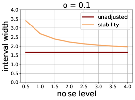
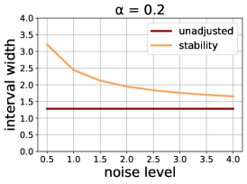
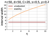
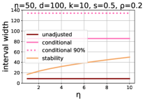
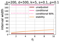
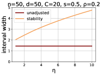
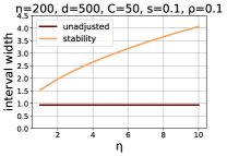
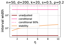
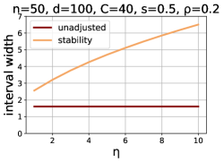
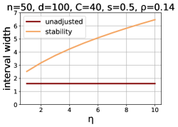
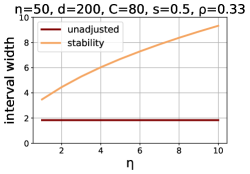
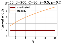
Figure 3: Normalized interval width implied by stability solution and unadjusted width for different noise levels b𝑏b and error levels α𝛼\alpha. We fix ν=0.05𝜈0.05\nu=0.05.

Although in the main body of the paper we state the result when 𝒫y=𝒩(μ,σ2)subscript𝒫𝑦𝒩𝜇superscript𝜎2\mathcal{P}_{y}=\mathcal{N}(\mu,\sigma^{2}) for simplicity, the Laplace noise addition strategy is valid for arbitrary 𝒫ysubscript𝒫𝑦\mathcal{P}_{y}; only the expression for η𝜂\eta changes as a function of 𝒫ysubscript𝒫𝑦\mathcal{P}_{y}. In the Supplement we state a general version of Claim 5.

The proof of Claim 5 relies on showing that the selection to report is stable with respect to the oracle S^(yE)^𝑆subscriptsuperscript𝑦𝐸\hat{S}(y^{\prime}_{E}), and hence we can invoke Lemma 2.

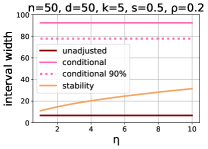
We can see that, by choosing ν0,bformulae-sequence𝜈0𝑏\nu\rightarrow 0,b\rightarrow\infty, we recover the non-selective confidence intervals, albeit at the cost of making the decision to report virtually independent of y𝑦y. As we decrease b𝑏b (and keep ν𝜈\nu bounded away from zero), the decision to report becomes more reflective of the event report(y)report𝑦\mathrm{report}(y) and the inference level smoothly becomes more stringent. In Figure 3 we plot the normalized interval width, z1α2(1ν)eηsubscript𝑧1𝛼21𝜈superscript𝑒𝜂z_{1-\frac{\alpha}{2}(1-\nu)e^{-\eta}}, together with the unadjusted normalized width z1α2subscript𝑧1𝛼2z_{1-\frac{\alpha}{2}}, for several different noise levels b𝑏b and error levels α𝛼\alpha and ν=0.05𝜈0.05\nu=0.05.

As a concrete example, suppose that report(y)={y>T}report𝑦𝑦𝑇\mathrm{report}(y)=\{y>T\}, for some threshold T𝑇T. Then, as in Claim 2 and Claim 4, we can conclude that 𝟏{report(y)}=𝟏{report(y+ξ)}1report𝑦1report𝑦𝜉\mathbf{1}\{\mathrm{report}(y)\}=\mathbf{1}\{\mathrm{report}(y+\xi)\} with probability 1δ1𝛿1-\delta over the choice of ξ𝜉\xi as long as b|yT|log(1/(2δ))𝑏𝑦𝑇12𝛿b\leq\frac{|y-T|}{\log(1/(2\delta))}.

8 The design of stable selection algorithms

We discuss general tools for designing stable selection methods and present an application of these tools to variable selection in linear regression. We begin with an overview of the basic properties of stability, which are key to efficient design of stable selections.

8.1 Properties of stability

Stability satisfies two key algorithmic properties: closure under post-processing and composition. We provide precise definitions of the two shortly. The reason why these properties enable efficient stability designs is that many selection rules can be written as post-processing and composition of simple computations, such as linear functions of the data or finding maxima of a sequence. As long as we know how to stabilize the necessary simple computations, closure under post-processing and composition provide rules for computing the overall stability parameter of the whole algorithm efficiently.

Post-processing.

First, stability is closed under post-processing: if 𝒜:n𝒮:𝒜superscript𝑛𝒮\mathcal{A}:\mathbb{R}^{n}\rightarrow\mathcal{S} is (η,τ,ν)𝜂𝜏𝜈(\eta,\tau,\nu)-stable, then for any (possibly randomized) map :𝒮𝒢:𝒮𝒢\mathcal{B}:\mathcal{S}\rightarrow\mathcal{G}, the composition 𝒜𝒜\mathcal{B}\leavevmode\nobreak\ \circ\leavevmode\nobreak\ \mathcal{A} is also (η,τ,ν)𝜂𝜏𝜈(\eta,\tau,\nu)-stable. While the proof of this fact is a straightforward consequence of the definition of stability, the implications are significant. Suppose for the moment that the statistician is given a stable version of the LASSO algorithm, and denote its solution by θ^LASSOsubscript^𝜃LASSO\hat{\theta}_{\mathrm{LASSO}}. Since θ^LASSOsubscript^𝜃LASSO\hat{\theta}_{\text{LASSO}} is stable, then so is

M^={j[d]:θ^LASSO,j0}.^𝑀conditional-set𝑗delimited-[]𝑑subscript^𝜃LASSO𝑗0\hat{M}=\{j\in[d]\leavevmode\nobreak\ :\leavevmode\nobreak\ \hat{\theta}_{\text{LASSO},j}\neq 0\}.

In fact, the statistician need not necessarily choose the model corresponding exactly to the support of θ^LASSOsubscript^𝜃LASSO\hat{\theta}_{\mathrm{LASSO}}; for example, they could choose M^={j[d]:|θ^LASSO,j|ϵ}^𝑀conditional-set𝑗delimited-[]𝑑subscript^𝜃LASSO𝑗italic-ϵ\hat{M}=\{j\in[d]:|\hat{\theta}_{\text{LASSO},j}|\geq\epsilon\}, for some constant threshold ϵitalic-ϵ\epsilon, or they could pick dseldsubscript𝑑sel𝑑d_{\mathrm{sel}}\leq d entries with the maximum absolute value. More generally, any model chosen solely as a function of θ^LASSOsubscript^𝜃LASSO\hat{\theta}_{\mathrm{LASSO}} inherits the same stability parameters as θ^LASSOsubscript^𝜃LASSO\hat{\theta}_{\mathrm{LASSO}}. And, according to Corollary 1, the same PoSI constant suffices to correct the confidence intervals resulting from any such model.

Composition.

The second important property is composition. In Algorithm 1, we define adaptive composition, after which we discuss simpler, non-adaptive composition.

input: data yn𝑦superscript𝑛y\in\mathbb{R}^{n}, sequence of algorithms 𝒜t:𝒮1××𝒮t1×n𝒮t,t[k]:subscript𝒜𝑡formulae-sequencesubscript𝒮1subscript𝒮𝑡1superscript𝑛subscript𝒮𝑡𝑡delimited-[]𝑘\mathcal{A}_{t}:\mathcal{S}_{1}\times\dots\times\mathcal{S}_{t-1}\times\mathbb{R}^{n}\rightarrow\mathcal{S}_{t},\leavevmode\nobreak\ t\in[k]

output: (a1,,ak)𝒮1××𝒮ksubscript𝑎1subscript𝑎𝑘subscript𝒮1subscript𝒮𝑘(a_{1},\dots,a_{k})\in\mathcal{S}_{1}\times\dots\times\mathcal{S}_{k}

for t=1,2,,k𝑡12𝑘t=1,2,\dots,k do

       Compute at=𝒜t(a1,,at1,y)𝒮tsubscript𝑎𝑡subscript𝒜𝑡subscript𝑎1subscript𝑎𝑡1𝑦subscript𝒮𝑡a_{t}=\mathcal{A}_{t}(a_{1},\dots,a_{t-1},y)\in\mathcal{S}_{t}
end for
Return (a1,,ak)subscript𝑎1subscript𝑎𝑘(a_{1},\dots,a_{k})
Algorithm 1 Adaptive composition

Adaptive composition consists of k𝑘k sequential rounds in which the analyst observes the outcomes of all previous computations and selects the next computation adaptively—as a function of the previous evaluations. The adaptive composition property bounds the stability parameters of Algorithm 1 in terms of the stability parameters of 𝒜tsubscript𝒜𝑡\mathcal{A}_{t}. In its simplest form, it says that Algorithm 1 is (kη,0,0)𝑘𝜂00(k\eta,0,0)-stable if for all t[k]𝑡delimited-[]𝑘t\in[k], 𝒜t(a1,,at1,)subscript𝒜𝑡subscript𝑎1subscript𝑎𝑡1\mathcal{A}_{t}(a_{1},\dots,a_{t-1},\cdot) is (η,0,0)𝜂00(\eta,0,0)-stable for all fixed a1,,at1subscript𝑎1subscript𝑎𝑡1a_{1},\dots,a_{t-1}. For example, for some selection algorithms such as forward stepwise, it is clear to see how they can be represented using adaptive composition. In forward stepwise, 𝒜tsubscript𝒜𝑡\mathcal{A}_{t} outputs an index it[d]subscript𝑖𝑡delimited-[]𝑑i_{t}\in[d], which corresponds to the variable i𝑖i that minimizes the squared error resulting from adding i𝑖i to the current pool of selected features; it=𝒜t(i1,,it1,y)subscript𝑖𝑡subscript𝒜𝑡subscript𝑖1subscript𝑖𝑡1𝑦i_{t}=\mathcal{A}_{t}(i_{1},\dots,i_{t-1},y). It suffices to prove that any given step of forward stepwise selection is stable, in order to infer that the overall algorithm is stable as well.

Our proofs will only require adaptive composition for algorithms with ν=0𝜈0\nu=0; such results follow from classical theory on differential privacy. More advanced (and naturally more conservative) adaptive composition theorems which allow ν>0𝜈0\nu>0 can be found in the context of typical stability [4]. In the Supplement we formally state the adaptive composition results we will need in our proofs.

A simpler kind of composition is non-adaptive composition. Here, the algorithms 𝒜tsubscript𝒜𝑡\mathcal{A}_{t} have no dependence on the past computations. Non-adaptive composition can capture a protocol that involves running multiple selection methods and choosing a final selection target as an arbitrary function of all the outputs. As we state formally in the Supplement, the resulting stability parameters simply add up. This is a rather appealing property of stability, as it suggests that the statistician only needs to keep track of the stability parameters of each selection algorithm they run, in order to derive valid selective confidence intervals. An analogous combination of the results of different selection methods was considered by Markovic and Taylor [38]; their approach, however, relies on a sophisticated Monte Carlo sampling scheme.

8.2 Model selection algorithms: examples

We now consider several algorithms for variable selection in linear regression through the lens of stability. While many of the principles presented in this section can be adapted to different distributional assumptions, for the sake of clarity and interpretability we assume that y𝒩(μ,σ2I)similar-to𝑦𝒩𝜇superscript𝜎2𝐼y\sim\mathcal{N}(\mu,\sigma^{2}I), where σ2superscript𝜎2\sigma^{2} is unknown but we have access to an estimate σ^2σ2χr2rsimilar-tosuperscript^𝜎2superscript𝜎2superscriptsubscript𝜒𝑟2𝑟\hat{\sigma}^{2}\sim\sigma^{2}\frac{\chi_{r}^{2}}{r}, independent of y𝑦y. This is the setup studied by Berk et al. [9]. More generally, we only need to know the decay of the tail of the distribution of y𝑦y in order to enforce stability. In the Supplement, we extend the algorithms in this section to the case of outcome vectors with a known bound on their Orlicz norm, for any Orlicz function. This includes cases such as general subgaussian and subexponential outcome vectors.

Model selection via the LASSO.

We begin by considering the canonical example of the LASSO estimator [55]. The LASSO estimate is the solution to the usual least-squares problem with an additional 1subscript1\ell_{1}-constraint on the regression coefficients:

θ^LASSOargminθd12yXθ22 s.t. θ1C1,subscript^𝜃LASSOsubscriptargmin𝜃superscript𝑑12superscriptsubscriptnorm𝑦𝑋𝜃22 s.t. subscriptnorm𝜃1subscript𝐶1\hat{\theta}_{\mathrm{LASSO}}\in\operatorname*{arg\,min}_{\theta\in\mathbb{R}^{d}}\frac{1}{2}\|y-X\theta\|_{2}^{2}\text{ s.t. }\|\theta\|_{1}\leq C_{1}, (5)

where C1>0subscript𝐶10C_{1}>0 is a tuning parameter. This problem is sometimes referred to as the LASSO in constrained/bound form, to contrast it with the LASSO in penalized form:

θ^LASSOλargminθd12yXθ22+λθ1,superscriptsubscript^𝜃LASSO𝜆subscriptargmin𝜃superscript𝑑12superscriptsubscriptnorm𝑦𝑋𝜃22𝜆subscriptnorm𝜃1\hat{\theta}_{\mathrm{LASSO}}^{\lambda}\in\operatorname*{arg\,min}_{\theta\in\mathbb{R}^{d}}\frac{1}{2}\|y-X\theta\|_{2}^{2}+\lambda\|\theta\|_{1}, (6)

where λ>0𝜆0\lambda>0 is now the tuning parameter. These two problems are equivalent: for any C1>0subscript𝐶10C_{1}>0, there exists a corresponding λ>0𝜆0\lambda>0 such that θ^LASSOsubscript^𝜃LASSO\hat{\theta}_{\mathrm{LASSO}} is an optimal solution for the problem in Eq. (6), and vice versa. In our analysis we focus on the formulation (5).

The LASSO objective induces sparse solutions, and a common way of declaring that a feature is relevant is to check for a corresponding non-zero entry in the LASSO solution vector. That is, the model “selected” by the LASSO is:

M^={j[d]:θ^LASSO,j0}.^𝑀conditional-set𝑗delimited-[]𝑑subscript^𝜃LASSO𝑗0\hat{M}=\{j\in[d]\leavevmode\nobreak\ :\leavevmode\nobreak\ \hat{\theta}_{\text{LASSO},j}\neq 0\}.

Model selection via the LASSO has been of great interest in prior work on selective inference, starting with Lee et al. [35]. While this work provides exact confidence intervals, it has been observed that these intervals (which do not make use of randomization) have infinite expected length [29]. Subsequent work has improved upon these often large confidence intervals by choosing a better event to condition on [37], or by applying randomization [54, 53, 52, 30, 40, 39].

We now formulate a stable version of the LASSO algorithm. It is inspired by the differentially private LASSO algorithm of Talwar et al. [49], although the noise variables are calibrated somewhat differently due to different modeling assumptions.

We use eisubscript𝑒𝑖e_{i} to denote the i𝑖i-th standard basis vector in dsuperscript𝑑\mathbb{R}^{d}, and {±ei}i=1dsuperscriptsubscriptplus-or-minussubscript𝑒𝑖𝑖1𝑑\{\pm e_{i}\}_{i=1}^{d} to denote the set of 2d2𝑑2d standard basis vectors, multiplied by 111 and 11-1. We also let X2,subscriptnorm𝑋2\|X\|_{2,\infty} denote the L2,subscript𝐿2L_{2,\infty} norm of X𝑋X, X2,:=maxi[d]Xi2assignsubscriptnorm𝑋2subscript𝑖delimited-[]𝑑subscriptnormsubscript𝑋𝑖2\|X\|_{2,\infty}:=\max_{i\in[d]}\|X_{i}\|_{2}.

input: design matrix Xn×d𝑋superscript𝑛𝑑X\in\mathbb{R}^{n\times d}, outcome vector yn𝑦superscript𝑛y\in\mathbb{R}^{n}, variance estimate σ^2σ2χr2rsimilar-tosuperscript^𝜎2superscript𝜎2superscriptsubscript𝜒𝑟2𝑟\hat{\sigma}^{2}\sim\sigma^{2}\frac{\chi_{r}^{2}}{r}, 1subscript1\ell_{1}-constraint C1subscript𝐶1C_{1}, number of steps k𝑘k, parameters δ(0,1),η>0formulae-sequence𝛿01𝜂0\delta\in(0,1),\eta>0

output: LASSO solution θ^LASSOdsubscript^𝜃LASSOsuperscript𝑑\hat{\theta}_{\mathrm{LASSO}}\in\mathbb{R}^{d}
Initialize θ1=0subscript𝜃10\theta_{1}=0
for t=1,2,,k𝑡12𝑘t=1,2,\dots,k do

        ϕC1{±ei}i=1dfor-allitalic-ϕsubscript𝐶1superscriptsubscriptplus-or-minussubscript𝑒𝑖𝑖1𝑑\forall\phi\in C_{1}\cdot\{\pm e_{i}\}_{i=1}^{d}, sample ξt,ϕi.i.d.Lap(4tr,1δ/(2d)C1X2,ηn)superscriptsimilar-toi.i.d.subscript𝜉𝑡italic-ϕLap4subscript𝑡𝑟1𝛿2𝑑subscript𝐶1subscriptnorm𝑋2𝜂𝑛\xi_{t,\phi}\stackrel{{\scriptstyle\text{i.i.d.}}}{{\sim}}\text{Lap}\left(\frac{4t_{r,1-\delta/(2d)}C_{1}\|X\|_{2,\infty}}{\eta n}\right)
ϕC1{±ei}i=1dfor-allitalic-ϕsubscript𝐶1superscriptsubscriptplus-or-minussubscript𝑒𝑖𝑖1𝑑\forall\phi\in C_{1}\cdot\{\pm e_{i}\}_{i=1}^{d}, let αϕ=2nσ^ϕX(yXθt)+ξt,ϕsubscript𝛼italic-ϕ2𝑛^𝜎superscriptitalic-ϕtopsuperscript𝑋top𝑦𝑋subscript𝜃𝑡subscript𝜉𝑡italic-ϕ\alpha_{\phi}=-\frac{2}{n\hat{\sigma}}\phi^{\top}X^{\top}(y-X\theta_{t})+\xi_{t,\phi}
Set ϕt=argminϕC1{±ei}i=1dαϕsubscriptitalic-ϕ𝑡subscriptargminitalic-ϕsubscript𝐶1superscriptsubscriptplus-or-minussubscript𝑒𝑖𝑖1𝑑subscript𝛼italic-ϕ\phi_{t}=\operatorname*{arg\,min}_{\phi\in C_{1}\cdot\{\pm e_{i}\}_{i=1}^{d}}\alpha_{\phi}
Set θt+1=(1Δt)θt+Δtϕtsubscript𝜃𝑡11subscriptΔ𝑡subscript𝜃𝑡subscriptΔ𝑡subscriptitalic-ϕ𝑡\theta_{t+1}=(1-\Delta_{t})\theta_{t}+\Delta_{t}\phi_{t}, where Δt=2t+1subscriptΔ𝑡2𝑡1\Delta_{t}=\frac{2}{t+1}
end for
Return θ^LASSO=θk+1subscript^𝜃LASSOsubscript𝜃𝑘1\hat{\theta}_{\mathrm{LASSO}}=\theta_{k+1}
Algorithm 2 Stable LASSO algorithm

In essence, Algorithm 2 is a randomized version of the classical Frank-Wolfe algorithm from constrained optimization [25].

We now argue that θ^LASSOsubscript^𝜃LASSO\hat{\theta}_{\mathrm{LASSO}} is stable. The proof is based on a composition argument: namely, we can view θ^LASSOsubscript^𝜃LASSO\hat{\theta}_{\mathrm{LASSO}} as the result of a composition of k𝑘k subroutines, each given by one optimization step which produces θtsubscript𝜃𝑡\theta_{t}. The stability of each subroutine is proved by extending an argument related to the “report noisy max” mechanism from differential privacy [17]. The full proof of Proposition 2 can be found in the Supplement.

Proposition 2 (LASSO stability).

Algorithm 2 is both

  • (a)

    (12kη2+2klog(1/δ)η,δ,δ)12𝑘superscript𝜂22𝑘1𝛿𝜂𝛿𝛿\left(\frac{1}{2}k\eta^{2}+\sqrt{2k\log(1/\delta)}\eta,\delta,\delta\right)-stable, and

  • (b)

    (kη,0,δ)𝑘𝜂0𝛿(k\eta,0,\delta)-stable.

We state two rates because there exist parameter regimes where either rate leads to tighter confidence intervals than the other (the first rate being tighter when η𝜂\eta is small).

By the post-processing property, Proposition 2 implies stability of any model M^^𝑀\hat{M} obtained as a function of θ^LASSOsubscript^𝜃LASSO\hat{\theta}_{\mathrm{LASSO}}, such as the model corresponding to its non-zero entries.

Notice that the noise level in Algorithm 2 is an explicit function of η𝜂\eta. This allows the statistician to understand the loss in utility—that is, how much worse θ^LASSOsubscript^𝜃LASSO\hat{\theta}_{\mathrm{LASSO}} is relative to an exact LASSO solution—due to randomization. In fact, building on work by Jaggi [27] and Talwar et al. [49], we can upper bound the excess risk resulting from randomization.

Proposition 3 (LASSO utility).

Suppose we run Algorithm 2 for k=nX2C1ησ^X2,𝑘𝑛superscriptsubscriptnorm𝑋2subscript𝐶1𝜂^𝜎subscriptnorm𝑋2k=\left\lceil\frac{n\|X\|_{\infty}^{2}C_{1}\eta}{\hat{\sigma}\|X\|_{2,\infty}}\right\rceil steps. Then,

1n𝔼[yXθ^LASSO22|y]minθ:θ1C11nyXθ22=O~(C1X2,log(d)tr,1δ/(2d)σnη).1𝑛𝔼delimited-[]conditionalsuperscriptsubscriptnorm𝑦𝑋subscript^𝜃LASSO22𝑦subscript:𝜃subscriptnorm𝜃1subscript𝐶11𝑛superscriptsubscriptnorm𝑦𝑋𝜃22~𝑂subscript𝐶1subscriptnorm𝑋2𝑑subscript𝑡𝑟1𝛿2𝑑𝜎𝑛𝜂\frac{1}{n}\mathbb{E}[\|y-X\hat{\theta}_{\mathrm{LASSO}}\|_{2}^{2}\leavevmode\nobreak\ |\leavevmode\nobreak\ y]-\min_{\theta:\|\theta\|_{1}\leq C_{1}}\frac{1}{n}\|y-X\theta\|_{2}^{2}=\tilde{O}\left(\frac{C_{1}\|X\|_{2,\infty}\log(d)t_{r,1-\delta/(2d)}\sigma}{n\eta}\right).

The proof is deferred to the Supplement.

Model selection via marginal screening.

One of the most commonly used model selection methods involves simply picking a constant number of the features with the largest absolute inner product with the outcome y𝑦y [26, 23]. That is, one selects features i𝑖i corresponding to the top k𝑘k values of |Xiy|superscriptsubscript𝑋𝑖top𝑦|X_{i}^{\top}y|, for a pre-specified parameter k𝑘k. This strategy is known as marginal screening, and it was first analyzed in the context of selective inference by Lee and Taylor [34].

In Algorithm 3, we state a stable version of marginal screening. Notice that the randomization scheme is similar to that of the stable LASSO method. As before, we let X2,subscriptnorm𝑋2\|X\|_{2,\infty} denote the L2,subscript𝐿2L_{2,\infty} norm of X𝑋X.

input: design matrix Xn×d𝑋superscript𝑛𝑑X\in\mathbb{R}^{n\times d}, outcome vector yn𝑦superscript𝑛y\in\mathbb{R}^{n}, variance estimate σ^2σ2χr2rsimilar-tosuperscript^𝜎2superscript𝜎2superscriptsubscript𝜒𝑟2𝑟\hat{\sigma}^{2}\sim\sigma^{2}\frac{\chi_{r}^{2}}{r}, model size k𝑘k, parameters δ(0,1),η>0formulae-sequence𝛿01𝜂0\delta\in(0,1),\eta>0

output: M^={i1,,ik}^𝑀subscript𝑖1subscript𝑖𝑘\hat{M}=\{i_{1},\dots,i_{k}\}
Compute (c1,,cd)=1nσ^Xydsubscript𝑐1subscript𝑐𝑑1𝑛^𝜎superscript𝑋top𝑦superscript𝑑(c_{1},\dots,c_{d})=\frac{1}{n\hat{\sigma}}X^{\top}y\in\mathbb{R}^{d}
res1=[d]subscriptres1delimited-[]𝑑\text{res}_{1}=[d]
for t=1,2,,k𝑡12𝑘t=1,2,\dots,k do

        iresifor-all𝑖subscriptres𝑖\forall i\in\text{res}_{i}, sample ξt,ii.i.d.Lap(2tr,1δ/(2d)X2,nη)superscriptsimilar-toi.i.d.subscript𝜉𝑡𝑖Lap2subscript𝑡𝑟1𝛿2𝑑subscriptnorm𝑋2𝑛𝜂\xi_{t,i}\stackrel{{\scriptstyle\text{i.i.d.}}}{{\sim}}\text{Lap}\left(\frac{2t_{r,1-\delta/(2d)}\|X\|_{2,\infty}}{n\eta}\right)
it=argmaxirest|ci+ξt,i|subscript𝑖𝑡subscriptargmax𝑖subscriptres𝑡subscript𝑐𝑖subscript𝜉𝑡𝑖i_{t}=\operatorname*{arg\,max}_{i\in\text{res}_{t}}|c_{i}+\xi_{t,i}|
rest+1=restitsubscriptres𝑡1subscriptres𝑡subscript𝑖𝑡\text{res}_{t+1}=\text{res}_{t}\setminus i_{t}
end for
Return M^={i1,,ik}^𝑀subscript𝑖1subscript𝑖𝑘\hat{M}=\{i_{1},\dots,i_{k}\}
Algorithm 3 Stable marginal screening algorithm

The high-level idea behind the proof of stability of Algorithm 3 is similar to that of Algorithm 2, and we present it in the Supplement.

Proposition 4 (Marginal screening stability).

Algorithm 3 is both

  • (a)

    (12kη2+2klog(1/δ)η,δ,δ)12𝑘superscript𝜂22𝑘1𝛿𝜂𝛿𝛿\left(\frac{1}{2}k\eta^{2}+\sqrt{2k\log(1/\delta)}\eta,\delta,\delta\right)-stable, and

  • (b)

    (kη,0,δ)𝑘𝜂0𝛿(k\eta,0,\delta)-stable.

As for the LASSO, we aim to quantify the loss in utility due to randomization. Given that the goal of marginal screening is to detect the largest k𝑘k values |ci|=|Xiy|subscript𝑐𝑖superscriptsubscript𝑋𝑖top𝑦|c_{i}|=|X_{i}^{\top}y|, a reasonable notion of utility loss is the difference between the values cisubscript𝑐𝑖c_{i} corresponding to the variables in M^^𝑀\hat{M}, and the actual largest values of cisubscript𝑐𝑖c_{i}.

Proposition 5 (Marginal screening utility).

Let misubscript𝑚𝑖m_{i} denote the index of the i𝑖i-th largest value cjsubscript𝑐𝑗c_{j} in absolute value, so that (|cm1|,,|cmd|)subscript𝑐subscript𝑚1subscript𝑐subscript𝑚𝑑(|c_{m_{1}}|,\dots,|c_{m_{d}}|) is the decreasing order statistic of {|ci|}i=1dsuperscriptsubscriptsubscript𝑐𝑖𝑖1𝑑\{|c_{i}|\}_{i=1}^{d}. Then, for any δ(0,1)superscript𝛿01\delta^{\prime}\in(0,1), Algorithm 3 satisfies:

{maxj[k]|cmj||cij|4tr,1δ/(2d)log(dk/δ)X2,nη|y}1δ.\mathbb{P}\!\left\{{\max_{j\in[k]}|c_{m_{j}}|-|c_{i_{j}}|\leq\frac{4t_{r,1-\delta/(2d)}\log(dk/\delta^{\prime})\|X\|_{2,\infty}}{n\eta}}\ \middle|\ {y}\right\}\geq 1-\delta^{\prime}.

9 Experimental results

In this section, we evaluate our selective intervals for the LASSO and marginal screening and compare our solution with data splitting.

For a fixed sample size n𝑛n we vary the number of features d𝑑d. We consider two different data-generating processes for the design matrix: one in which the rows of X𝑋X are drawn independently from an equicorrelated multivariate Gaussian distribution with pairwise correlation ρ=0.5𝜌0.5\rho=0.5, and the second one in which all entries of X𝑋X are drawn as independent Bernoulli random variables with parameter 0.10.10.1. In the former case, X𝑋X is normalized to have columns of unit norm. The outcome is generated as y=Xβ+ϵ𝑦𝑋𝛽italic-ϵy=X\beta+\epsilon, where ϵii.i.d.𝒩(0,1),i[n]\epsilon_{i}\stackrel{{\scriptstyle\mathrm{i.i.d.}}}{{\sim}}\mathcal{N}(0,1),i\in[n], and the entries of β𝛽\beta are sampled according to

βi={Exp(ρ),i{1,,sd},0,i{sd+1,,d},subscript𝛽𝑖casesExp𝜌𝑖1𝑠𝑑otherwise0𝑖𝑠𝑑1𝑑otherwise\beta_{i}=\begin{cases}\mathrm{Exp}(\rho),\leavevmode\nobreak\ i\in\{1,\dots,sd\},\\ 0,\leavevmode\nobreak\ i\in\{sd+1,\dots,d\},\end{cases}

for a signal parameter ρ>0𝜌0\rho>0 and a sparsity parameter s(0,1)𝑠01s\in(0,1), which we vary. In the Supplement we provide additional experiments when the errors are drawn from a heavier-tailed, Laplace distribution. We fix the target miscoverage level to be α=0.1𝛼0.1\alpha=0.1. In all experiments we vary η{1,2,3,4,5,6,7,8,9,10}𝜂12345678910\eta\in\{1,2,3,4,5,6,7,8,9,10\}. For the comparison with data splitting, we use the splitting fraction derived in Section 5.1. Further experimental details are given in the Supplement.
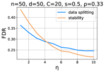
Refer to caption Refer to caption Refer to caption Refer to caption

Refer to caption Refer to caption Refer to caption Refer to caption

Refer to caption Refer to caption Refer to caption Refer to caption

Figure 4: Comparison of FDR after stable LASSO and LASSO with data splitting, with varying dimension and signal strength, in the Gaussian design case. In addition, we plot the average interval width (at ρ=0.2𝜌0.2\rho=0.2 only, however the width varies minimally with ρ𝜌\rho) and the average unadjusted width.

Refer to caption Refer to caption Refer to caption Refer to caption

Figure 5: Comparison of FDR after stable LASSO and LASSO with data splitting, with varying sample size, in the Gaussian design case. In addition, we plot the average interval width at n=200𝑛200n=200 and the average unadjusted width.

9.1 Gaussian design

We first state the results for the Gaussian design case.

LASSO.

In Figure 4 we compare the false discovery rate (FDR) of the stable LASSO algorithm and the LASSO algorithm with data splitting. In all plots n=50𝑛50n=50 is fixed and we vary d{50,100,200}𝑑50100200d\in\{50,100,200\}. As we increase d𝑑d, we also increase the size of the constraint set C1{20,40,80}subscript𝐶1204080C_{1}\in\{20,40,80\} to allow more selections. We consider signal levels ρ{0.33,0.2,0.14}𝜌0.330.20.14\rho\in\{0.33,0.2,0.14\}, which corresponds to an expected value of the non-null βisubscript𝛽𝑖\beta_{i} lying in {3,5,7}357\{3,5,7\}, and we fix s=0.5𝑠0.5s=0.5.

We observe that stability generally outperforms data splitting as η𝜂\eta grows, equivalently when the splitting fraction f(η)𝑓𝜂f(\eta) grows, as well as when the signal strength grows. In Figure 4 we additionally plot the average width of stable intervals against the average width of naive, unadjusted intervals. Note that the intervals obtained via data splitting have essentially the same width (and are hence not plotted), based on how f(η)𝑓𝜂f(\eta) is chosen. We only plot interval width for ρ=0.2𝜌0.2\rho=0.2 since the width varies minimally for different values of ρ𝜌\rho. For completeness we include all plots of interval width in the Supplement.
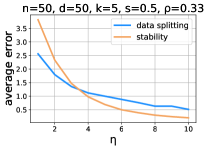
Refer to caption Refer to caption Refer to caption Refer to caption

Refer to caption Refer to caption Refer to caption Refer to caption

Refer to caption Refer to caption Refer to caption Refer to caption

Figure 6: Comparison of average error after stable marginal screening and marginal screening with data splitting, with varying dimension and signal strength, in the Gaussian design case. In addition, we plot the average interval width (at ρ=0.2𝜌0.2\rho=0.2 only, however the width varies minimally with ρ𝜌\rho), together with the average unadjusted width and the width obtained via the conditional correction of Lee and Taylor [34]. We also plot the 90%percent9090\% quantile of the conditional width because it varies greatly across realizations.

Refer to caption Refer to caption Refer to caption Refer to caption

Figure 7: Comparison of average error after stable marginal screening and marginal screening with data splitting, with varying sample size, in the Gaussian design case. In addition, we plot the average interval width at n=200𝑛200n=200, together with the average unadjusted width and the width implied by the conditional approach of Lee and Taylor [34].

In Figure 5 we compare the stable LASSO algorithm and the LASSO with data splitting in a sparse high-dimensional setting with d=500,s=0.1formulae-sequence𝑑500𝑠0.1d=500,s=0.1, and we vary the sample size n{100,200,300}𝑛100200300n\in\{100,200,300\}. We fix ρ=0.1𝜌0.1\rho=0.1. We observe that stability consistently outperforms data splitting for large enough η𝜂\eta and this gap grows with n𝑛n. In addition, we plot the average interval width implied by stability against the average unadjusted interval width at n=200𝑛200n=200 (again we do not plot the interval width given by data splitting for the same reason as in Figure 4). We include the plots of all interval widths in the Supplement.

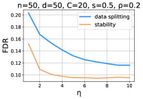
Refer to caption Refer to caption Refer to caption Refer to caption

Refer to caption Refer to caption Refer to caption Refer to caption

Refer to caption Refer to caption Refer to caption Refer to caption

Figure 8: Comparison of FDR after stable LASSO and LASSO with data splitting, with varying dimension and signal strength, in the Bernoulli design case. In addition, we plot the average interval width (at ρ=0.2𝜌0.2\rho=0.2 only, however the width varies minimally with ρ𝜌\rho) and the average unadjusted width.

Refer to caption Refer to caption Refer to caption Refer to caption

Figure 9: Comparison of FDR after stable LASSO and LASSO with data splitting, with varying sample size, in the Bernoulli design case. In addition, we plot the average interval width at n=200𝑛200n=200 and the average unadjusted width.

Marginal screening.

In Figure 6 we compare the average error of stable marginal screening and marginal screening with data splitting. Since marginal screening explicitly aims to maximize the values |Xiy|superscriptsubscript𝑋𝑖top𝑦|X_{i}^{\top}y| for selected variables Xisubscript𝑋𝑖X_{i}, we quantify the error as 1kt=1k(|Xity||Xity|)1𝑘superscriptsubscript𝑡1𝑘superscriptsubscript𝑋superscriptsubscript𝑖𝑡top𝑦superscriptsubscript𝑋subscript𝑖𝑡top𝑦\frac{1}{k}\sum_{t=1}^{k}(|X_{i_{t}^{*}}^{\top}y|-|X_{i_{t}}^{\top}y|), where itsubscript𝑖𝑡i_{t} is the estimated index of the t𝑡t-th largest absolute inner product (based on a subsample in the case of data splitting, or based on a randomized sample in the case of stability), and itsuperscriptsubscript𝑖𝑡i_{t}^{*} is the true index of the t𝑡t-th largest absolute inner product in the data set. We vary the parameters as in the LASSO comparison in Figure 4, only instead of varying C1subscript𝐶1C_{1} we vary k{5,10,20}𝑘51020k\in\{5,10,20\}. We also plot the average interval width with stability, together with the unadjusted interval width and the average width obtained via the conditional method of Lee and Taylor [34] with no randomization. For the conditional method, since the intervals are sometimes orders of magnitude larger than the average width, we also plot the 90%percent9090\% quantile of interval width. We see that stability typically outperforms data splitting in terms of the average error, and this benefit is more pronounced for larger η𝜂\eta and signal strength. In terms of interval width, we observe that stability leads to significantly smaller intervals than the conditional approach. We only plot interval width when ρ=0.2𝜌0.2\rho=0.2, and defer the remaining plots to the Supplement.

In Figure 7 we consider a setting analogous to that of Figure 5, and we analogously vary the sample size n𝑛n. We again see that stability generally dominates data splitting. Moreover, the gap between the intervals obtained via stability and those of Lee and Taylor [34] is even more pronounced than in Figure 6. We provide the plots of all interval widths in the Supplement.

9.2 Bernoulli design

Now we consider the Bernoulli design case. The motivation for considering a sparse Bernoulli design lies in the fact that certain directions in the column space of X𝑋X are captured by only a few samples, hence missing out on them—as is possible with data splitting—can significantly affect the quality of selection.

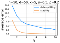
Refer to caption Refer to caption Refer to caption Refer to caption

Refer to caption Refer to caption Refer to caption Refer to caption

Refer to caption Refer to caption Refer to caption Refer to caption

Figure 10: Comparison of average error after stable marginal screening and marginal screening with data splitting, with varying dimension and signal strength, in the Bernoulli design case. In addition, we plot the average interval width (at ρ=0.2𝜌0.2\rho=0.2 only, however the width varies minimally with ρ𝜌\rho), together with the average unadjusted width and the width obtained via the conditional correction of Lee and Taylor [34]. We also plot the 90%percent9090\% quantile of the conditional width because it varies greatly across realizations. Since the conditional widths are of a higher order of magnitude, the scale on the y𝑦y-axis in the widths plots is logarithmic.

Refer to caption Refer to caption Refer to caption Refer to caption

Figure 11: Comparison of average error after stable marginal screening and marginal screening with data splitting, with varying sample size, in the Bernoulli design case. In addition, we plot the average interval width at n=200𝑛200n=200, together with the average unadjusted width and the width implied by the conditional approach of Lee and Taylor [34]. Since the conditional widths are of a higher order of magnitude, the scale on the y𝑦y-axis in the widths plot is logarithmic.

LASSO.

In Figure 8 and Figure 9 we provide comparisons analogous to those of Figure 4 and Figure 5, using the same parameter configurations. We observe a larger gap between data splitting and stability than in the Gaussian design case, and observe the same trends: as η𝜂\eta and the signal strength grow, the performance gap increases. As before, we defer the remaining plots of interval widths to the Supplement.

Marginal screening.

In Figure 10 and Figure 11 we provide comparisons analogous to those of Figure 6 and Figure 7, using the same parameter configurations. We observe a larger gap between data splitting and stability both than in the Gaussian design case, as well as in the LASSO experiments using the Bernoulli design. In addition, we observe an even more pronounced gap between stable confidence interval widths and widths of intervals obtained via a conditional correction [34]. For this reason, the y𝑦y-axis in the widths plots is logarithmic. We defer the remaining plots of interval widths to the Supplement.

10 Discussion

Building on concepts from algorithmic stability, as originally developed for applications in differential privacy, we have provided general theory for designing post-selection confidence intervals when the selection procedure is stable. The stability principle is broadly applicable, ranging from inference on the winning effect to model selection in linear regression. In particular, stability is applicable even when data splitting is not, such as when there are dependencies between observations.

Performing inference after a stable selection is simple: it merely requires discounting the type I error based on the level of stability. Moreover, stability comes with several practically appealing properties, namely robustness to post-processing and composition. Thus, for example, the statistician can run various selection methods, and essentially only needs to keep track of the stability parameters of each in order to obtain valid confidence intervals for the final target, which could combine the results of all the selections in an arbitrary way.

There are numerous other potential applications of algorithmic stability to the problem of post-selection inference that would be worthwhile to explore. For example, it would be valuable to understand bootstrapping [42] from the perspective of stability, due to its conceptual relations to the “privacy amplification by subsampling” principle in differential privacy, which argues that privacy is amplified when run on a random subsample of the entire data set [28, 6]. More broadly, selective mechanisms have been long analyzed in the context of differential privacy [51, 36, 48, 16, 22], and we believe that some of these developments could be imported to selective inference via stability.

Acknowledgements

We are grateful to Vitaly Feldman, Will Fithian, Moritz Hardt, Arun Kumar Kuchibhotla, and Adam Sealfon for many helpful discussions and feedback which has lead to improvements of this work. In particular, we thank Will Fithian for pointing out the advantages of the oracle definition of stability. This work was supported by the Army Research Office (ARO) under contract W911NF-17-1-0304 as part of the collaboration between US DOD, UK MOD and UK Engineering and Physical Research Council (EPSRC) under the Multidisciplinary University Research Initiative (MURI).

References

  • Andrews et al. [2019] Isaiah Andrews, Toru Kitagawa, and Adam McCloskey. Inference on winners. National Bureau of Economic Research, 2019.
  • Bachoc et al. [2020] François Bachoc, David Preinerstorfer, and Lukas Steinberger. Uniformly valid confidence intervals post-model-selection. Annals of Statistics, 48(1):440–463, 2020.
  • Barber et al. [2021] Rina Foygel Barber, Emmanuel J Candes, Aaditya Ramdas, and Ryan J Tibshirani. Predictive inference with the jackknife+. Annals of Statistics, 49(1):486–507, 2021.
  • Bassily and Freund [2016] Raef Bassily and Yoav Freund. Typical stability. arXiv preprint arXiv:1604.03336, 2016.
  • Bassily et al. [2016] Raef Bassily, Kobbi Nissim, Adam Smith, Thomas Steinke, Uri Stemmer, and Jonathan Ullman. Algorithmic stability for adaptive data analysis. In Proceedings of the 48th Annual ACM Symposium on Theory of Computing (STOC), pages 1046–1059, 2016.
  • Beimel et al. [2010] Amos Beimel, Shiva Prasad Kasiviswanathan, and Kobbi Nissim. Bounds on the sample complexity for private learning and private data release. In Theory of Cryptography Conference, pages 437–454. Springer, 2010.
  • Benjamini [2010] Yoav Benjamini. Simultaneous and selective inference: Current successes and future challenges. Biometrical Journal, 52(6):708–721, 2010.
  • Benjamini et al. [2019] Yoav Benjamini, Yotam Hechtlinger, and Philip B Stark. Confidence intervals for selected parameters. arXiv preprint arXiv:1906.00505, 2019.
  • Berk et al. [2013] Richard Berk, Lawrence Brown, Andreas Buja, Kai Zhang, and Linda Zhao. Valid post-selection inference. Annals of Statistics, 41(2):802–837, 2013.
  • Bi et al. [2020] Nan Bi, Jelena Markovic, Lucy Xia, and Jonathan Taylor. Inferactive data analysis. Scandinavian Journal of Statistics, 47(1):212–249, 2020.
  • Bousquet and Elisseeff [2002] Olivier Bousquet and André Elisseeff. Stability and generalization. Journal of Machine Learning Research, 2(Mar):499–526, 2002.
  • Buja et al. [2019] Andreas Buja, Lawrence Brown, Richard Berk, Edward George, Emil Pitkin, Mikhail Traskin, Kai Zhang, and Linda Zhao. Models as approximations I: Consequences illustrated with linear regression. Statistical Science, 34(4):523–544, 2019.
  • Bun and Steinke [2016] Mark Bun and Thomas Steinke. Concentrated differential privacy: Simplifications, extensions, and lower bounds. In Theory of Cryptography Conference, pages 635–658. Springer, 2016.
  • Clarkson [2010] Kenneth L Clarkson. Coresets, sparse greedy approximation, and the Frank-Wolfe algorithm. ACM Transactions on Algorithms, 6(4):1–30, 2010.
  • Cummings et al. [2016] Rachel Cummings, Katrina Ligett, Kobbi Nissim, Aaron Roth, and Zhiwei Steven Wu. Adaptive learning with robust generalization guarantees. In Conference on Learning Theory (COLT), pages 772–814, 2016.
  • Durfee and Rogers [2019] David Durfee and Ryan M Rogers. Practical differentially private top-k selection with pay-what-you-get composition. In Advances in Neural Information Processing Systems (NeurIPS), pages 3532–3542, 2019.
  • Dwork and Roth [2014] Cynthia Dwork and Aaron Roth. The Algorithmic Foundations of Differential Privacy, volume 9. Now Publishers, Inc., 2014.
  • Dwork et al. [2006] Cynthia Dwork, Frank McSherry, Kobbi Nissim, and Adam Smith. Calibrating noise to sensitivity in private data analysis. In Theory of Cryptography Conference, pages 265–284. Springer, 2006.
  • Dwork et al. [2010] Cynthia Dwork, Guy N Rothblum, and Salil Vadhan. Boosting and differential privacy. In IEEE 51st Annual Symposium on Foundations of Computer Science (FOCS), pages 51–60, 2010.
  • Dwork et al. [2015a] Cynthia Dwork, Vitaly Feldman, Moritz Hardt, Toni Pitassi, Omer Reingold, and Aaron Roth. Generalization in adaptive data analysis and holdout reuse. In Advances in Neural Information Processing Systems (NIPS), pages 2350–2358, 2015a.
  • Dwork et al. [2015b] Cynthia Dwork, Vitaly Feldman, Moritz Hardt, Toniann Pitassi, Omer Reingold, and Aaron Leon Roth. Preserving statistical validity in adaptive data analysis. In Proceedings of the 47th Annual ACM Symposium on Theory of Computing (STOC), pages 117–126, 2015b.
  • Dwork et al. [2015c] Cynthia Dwork, Weijie Su, and Li Zhang. Private false discovery rate control. arXiv preprint arXiv:1511.03803, 2015c.
  • Fan and Lv [2008] Jianqing Fan and Jinchi Lv. Sure independence screening for ultrahigh dimensional feature space. Journal of the Royal Statistical Society: Series B (Statistical Methodology), 70(5):849–911, 2008.
  • Fithian et al. [2014] William Fithian, Dennis Sun, and Jonathan Taylor. Optimal inference after model selection. arXiv preprint arXiv:1410.2597, 2014.
  • Frank and Wolfe [1956] Marguerite Frank and Philip Wolfe. An algorithm for quadratic programming. Naval Research Logistics Quarterly, 3(1-2):95–110, 1956.
  • Guyon and Elisseeff [2003] Isabelle Guyon and André Elisseeff. An introduction to variable and feature selection. Journal of Machine Learning Research, 3(Mar):1157–1182, 2003.
  • Jaggi [2013] Martin Jaggi. Revisiting Frank-Wolfe: Projection-free sparse convex optimization. In Proceedings of the 30th International Conference on Machine Learning, pages 427–435, 2013.
  • Kasiviswanathan et al. [2011] Shiva Prasad Kasiviswanathan, Homin K Lee, Kobbi Nissim, Sofya Raskhodnikova, and Adam Smith. What can we learn privately? SIAM Journal on Computing, 40(3):793–826, 2011.
  • Kivaranovic and Leeb [2020a] Danijel Kivaranovic and Hannes Leeb. On the length of post-model-selection confidence intervals conditional on polyhedral constraints. Journal of the American Statistical Association, pages 1–13, 2020a.
  • Kivaranovic and Leeb [2020b] Danijel Kivaranovic and Hannes Leeb. A (tight) upper bound for the length of confidence intervals with conditional coverage. arXiv preprint arXiv:2007.12448, 2020b.
  • Kuchibhotla et al. [2019] Arun K Kuchibhotla, Lawrence D Brown, Andreas Buja, and Junhui Cai. All of linear regression. arXiv preprint arXiv:1910.06386, 2019.
  • Kuchibhotla et al. [2020a] Arun K Kuchibhotla, Lawrence D Brown, Andreas Buja, Junhui Cai, Edward I George, and Linda H Zhao. Valid post-selection inference in model-free linear regression. Annals of Statistics, 48(5):2953–2981, 2020a.
  • Kuchibhotla et al. [2020b] Arun Kumar Kuchibhotla, Alessandro Rinaldo, and Larry Wasserman. Berry-Esseen bounds for projection parameters and partial correlations with increasing dimension. arXiv preprint arXiv:2007.09751, 2020b.
  • Lee and Taylor [2014] Jason D Lee and Jonathan E Taylor. Exact post model selection inference for marginal screening. In Advances in Neural Information Processing Systems (NIPS), pages 136–144, 2014.
  • Lee et al. [2016] Jason D Lee, Dennis L Sun, Yuekai Sun, and Jonathan E Taylor. Exact post-selection inference, with application to the lasso. Annals of Statistics, 44(3):907–927, 2016.
  • Lei et al. [2018] Jing Lei, Anne Sophie Charest, Aleksandra Slavkovic, Adam Smith, and Stephen Fienberg. Differentially private model selection with penalized and constrained likelihood. Journal of the Royal Statistical Society. Series A: Statistics in Society, 181(3):609–633, 2018.
  • Liu et al. [2018] Keli Liu, Jelena Markovic, and Robert Tibshirani. More powerful post-selection inference, with application to the Lasso. arXiv preprint arXiv:1801.09037, 2018.
  • Markovic and Taylor [2016] Jelena Markovic and Jonathan Taylor. Bootstrap inference after using multiple queries for model selection. arXiv preprint arXiv:1612.07811, 2016.
  • Panigrahi and Taylor [2019] Snigdha Panigrahi and Jonathan Taylor. Approximate selective inference via maximum likelihood. arXiv preprint arXiv:1902.07884, 2019.
  • Panigrahi et al. [2017] Snigdha Panigrahi, Jelena Markovic, and Jonathan Taylor. An MCMC-free approach to post-selective inference. arXiv preprint arXiv:1703.06154, 2017.
  • Rasines and Young [2021] Daniel G Rasines and G Alastair Young. Splitting strategies for post-selection inference. arXiv preprint arXiv:2102.02159, 2021.
  • Rinaldo et al. [2019] Alessandro Rinaldo, Larry Wasserman, and Max G’Sell. Bootstrapping and sample splitting for high-dimensional, assumption-lean inference. Annals of Statistics, 47(6):3438–3469, 2019.
  • Rogers et al. [2016] Ryan Rogers, Aaron Roth, Adam Smith, and Om Thakkar. Max-information, differential privacy, and post-selection hypothesis testing. In IEEE 57th Annual Symposium on Foundations of Computer Science (FOCS), pages 487–494, 2016.
  • Rosenthal [1979] Robert Rosenthal. The file drawer problem and tolerance for null results. Psychological Bulletin, 86(3):638, 1979.
  • Russo and Zou [2016] Daniel Russo and James Zou. Controlling bias in adaptive data analysis using information theory. In Artificial Intelligence and Statistics, pages 1232–1240, 2016.
  • Scheffe [1999] Henry Scheffe. The Analysis of Variance. John Wiley & Sons, 1999.
  • Steinberger and Leeb [2018] Lukas Steinberger and Hannes Leeb. Conditional predictive inference for high-dimensional stable algorithms. arXiv preprint arXiv:1809.01412, 2018.
  • Steinke and Ullman [2017] Thomas Steinke and Jonathan Ullman. Tight lower bounds for differentially private selection. In IEEE 58th Annual Symposium on Foundations of Computer Science (FOCS), pages 552–563, 2017.
  • Talwar et al. [2015] Kunal Talwar, Abhradeep Guha Thakurta, and Li Zhang. Nearly optimal private LASSO. In Advances in Neural Information Processing Systems (NIPS), pages 3025–3033, 2015.
  • Taylor and Tibshirani [2015] Jonathan Taylor and Robert J Tibshirani. Statistical learning and selective inference. Proceedings of the National Academy of Sciences, 112(25):7629–7634, 2015.
  • Thakurta and Smith [2013] Abhradeep Guha Thakurta and Adam Smith. Differentially private feature selection via stability arguments, and the robustness of the lasso. In Conference on Learning Theory (COLT), pages 819–850, 2013.
  • Tian and Taylor [2018] Xiaoying Tian and Jonathan Taylor. Selective inference with a randomized response. Annals of Statistics, 46(2):679–710, 2018.
  • Tian et al. [2016] Xiaoying Tian, Nan Bi, and Jonathan Taylor. MAGIC: a general, powerful and tractable method for selective inference. arXiv preprint arXiv:1607.02630, 2016.
  • Tian Harris et al. [2016] Xiaoying Tian Harris, Snigdha Panigrahi, Jelena Markovic, Nan Bi, and Jonathan Taylor. Selective sampling after solving a convex problem. arXiv preprint arXiv:1609.05609, 2016.
  • Tibshirani [1996] Robert Tibshirani. Regression shrinkage and selection via the lasso. Journal of the Royal Statistical Society: Series B (Methodological), 58(1):267–288, 1996.
  • Tibshirani et al. [2016] Ryan J Tibshirani, Jonathan Taylor, Richard Lockhart, and Robert Tibshirani. Exact post-selection inference for sequential regression procedures. Journal of the American Statistical Association, 111(514):600–620, 2016.

Appendix A Proofs

A.1 Composition of stability

Here we summarize prior work on adaptive composition theorems for differential privacy, which will be crucial in our proofs. To facilitate readability, we restate the definition of adaptive composition.

input: data yn𝑦superscript𝑛y\in\mathbb{R}^{n}, sequence of algorithms 𝒜i:1××i1×ni,i[k]:subscript𝒜𝑖formulae-sequencesubscript1subscript𝑖1superscript𝑛subscript𝑖𝑖delimited-[]𝑘\mathcal{A}_{i}:\mathcal{F}_{1}\times\dots\times\mathcal{F}_{i-1}\times\mathbb{R}^{n}\rightarrow\mathcal{F}_{i},\leavevmode\nobreak\ i\in[k]

output: (a1,,ak)1××ksubscript𝑎1subscript𝑎𝑘subscript1subscript𝑘(a_{1},\dots,a_{k})\in\mathcal{F}_{1}\times\dots\times\mathcal{F}_{k}
for i=1,2,,k𝑖12𝑘i=1,2,\dots,k do

       Compute ai=𝒜i(a1,,ai1,y)isubscript𝑎𝑖subscript𝒜𝑖subscript𝑎1subscript𝑎𝑖1𝑦subscript𝑖a_{i}=\mathcal{A}_{i}(a_{1},\dots,a_{i-1},y)\in\mathcal{F}_{i}
end for
Return 𝒜(k)(y)=(a1,,ak)superscript𝒜𝑘𝑦subscript𝑎1subscript𝑎𝑘\mathcal{A}^{(k)}(y)=(a_{1},\dots,a_{k})
Algorithm 4 Adaptive composition

The first statement below is a reformulation of the “simple” composition property of differential privacy [18]. The second statement is a slightly stronger reformulation [13] of the so-called “advanced” composition theorem for differential privacy [19].

Lemma 3 ([19, 13]).

Fix two vectors y,yn𝑦superscript𝑦superscript𝑛y,y^{\prime}\in\mathbb{R}^{n} and suppose that 𝒜t(a1,,at1,y)η,τ𝒜t(a1,,at1,y)subscript𝜂𝜏subscript𝒜𝑡subscript𝑎1subscript𝑎𝑡1𝑦subscript𝒜𝑡subscript𝑎1subscript𝑎𝑡1superscript𝑦\mathcal{A}_{t}(a_{1},\dots,a_{t-1},y)\approx_{\eta,\tau}\mathcal{A}_{t}(a_{1},\dots,a_{t-1},y^{\prime}), for every fixed sequence a1,,at1subscript𝑎1subscript𝑎𝑡1a_{1},\dots,a_{t-1}, and all t[k]𝑡delimited-[]𝑘t\in[k]. Then,

  • (a)

    𝒜(k)(y)kη,kτ𝒜(k)(y)subscript𝑘𝜂𝑘𝜏superscript𝒜𝑘𝑦superscript𝒜𝑘superscript𝑦\mathcal{A}^{(k)}(y)\approx_{k\eta,k\tau}\mathcal{A}^{(k)}(y^{\prime}),

  • (b)

    𝒜(k)(y)12kη2+2klog(1/δ)η,kτ+δ𝒜(k)(y)subscript12𝑘superscript𝜂22𝑘1𝛿𝜂𝑘𝜏𝛿superscript𝒜𝑘𝑦superscript𝒜𝑘superscript𝑦\mathcal{A}^{(k)}(y)\approx_{\frac{1}{2}k\eta^{2}+\sqrt{2k\log(1/\delta)}\eta,k\tau+\delta}\mathcal{A}^{(k)}(y^{\prime}), for all δ(0,1)𝛿01\delta\in(0,1).

We also state a non-adaptive composition property of stability, which is relevant when running multiple model selection algorithms. It says that the privacy parameters of all outputs combined simply add up.

Lemma 4.

Suppose 𝒜i:ni:subscript𝒜𝑖superscript𝑛subscript𝑖\mathcal{A}_{i}:\mathbb{R}^{n}\rightarrow\mathcal{F}_{i} is (ηi,τi,νi)subscript𝜂𝑖subscript𝜏𝑖subscript𝜈𝑖(\eta_{i},\tau_{i},\nu_{i})-stable, for all i[k]𝑖delimited-[]𝑘i\in[k]. Then, 𝒜(k):n1××k:superscript𝒜𝑘superscript𝑛subscript1subscript𝑘\mathcal{A}^{(k)}:\leavevmode\nobreak\ \mathbb{R}^{n}\rightarrow\mathcal{F}_{1}\times\dots\times\mathcal{F}_{k} defined as 𝒜(k)()=(𝒜1(),,𝒜k())superscript𝒜𝑘subscript𝒜1subscript𝒜𝑘\mathcal{A}^{(k)}(\cdot)=(\mathcal{A}_{1}(\cdot),\dots,\mathcal{A}_{k}(\cdot)) is (i=1kηi,i=1kτi,i=1kνi)superscriptsubscript𝑖1𝑘subscript𝜂𝑖superscriptsubscript𝑖1𝑘subscript𝜏𝑖superscriptsubscript𝑖1𝑘subscript𝜈𝑖(\sum_{i=1}^{k}\eta_{i},\sum_{i=1}^{k}\tau_{i},\sum_{i=1}^{k}\nu_{i})-stable.

The proof of Lemma 4 follows by the simple composition theorem for differential privacy [19], together with a union bound over all failure events with probability νisubscript𝜈𝑖\nu_{i}.

A.2 Proof of Claim 1

Let E={ωn:ωμz1αδ/(2n)}𝐸conditional-set𝜔superscript𝑛subscriptnorm𝜔𝜇subscript𝑧1𝛼𝛿2𝑛E=\{\omega\in\mathbb{R}^{n}:\|\omega-\mu\|_{\infty}\leq z_{1-\alpha\delta/(2n)}\}. Then, by a Bonferroni correction, we know that {yE}1αδ𝑦𝐸1𝛼𝛿\mathbb{P}\!\left\{{y\in E}\right\}\geq 1-\alpha\delta.

For any ωn𝜔superscript𝑛\omega\in\mathbb{R}^{n}, let i^(ω)=argmaxi(ωi+ξi)subscript^𝑖𝜔subscriptargmax𝑖subscript𝜔𝑖subscript𝜉𝑖\hat{i}_{*}(\omega)=\operatorname*{arg\,max}_{i}(\omega_{i}+\xi_{i}), where ξii.i.d.Lap(2z1αδ/(2n)η)\xi_{i}\stackrel{{\scriptstyle\mathrm{i.i.d.}}}{{\sim}}\mathrm{Lap}\left(\frac{2z_{1-\alpha\delta/(2n)}}{\eta}\right). Define

ξ=argminξyi+ξi>yj+ξj,ji.formulae-sequencesuperscript𝜉subscriptargmin𝜉subscript𝑦𝑖subscript𝜉𝑖subscript𝑦𝑗subscript𝜉𝑗for-all𝑗𝑖\xi^{*}=\operatorname*{arg\,min}_{\xi}y_{i}+\xi_{i}>y_{j}+\xi_{j},\leavevmode\nobreak\ \forall j\neq i.

Then, i^(y)=isubscript^𝑖𝑦𝑖\hat{i}_{*}(y)=i if and only if ξiξsubscript𝜉𝑖superscript𝜉\xi_{i}\geq\xi^{*}. By the definition of E𝐸E we have that for all yE𝑦𝐸y\in E

z1αδ/(2n)+μi+ξyi+ξ>yj+ξjμj+ξjz1αδ/(2n),subscript𝑧1𝛼𝛿2𝑛subscript𝜇𝑖superscript𝜉subscript𝑦𝑖superscript𝜉subscript𝑦𝑗subscript𝜉𝑗subscript𝜇𝑗subscript𝜉𝑗subscript𝑧1𝛼𝛿2𝑛\displaystyle z_{1-\alpha\delta/(2n)}+\mu_{i}+\xi^{*}\geq y_{i}+\xi^{*}>y_{j}+\xi_{j}\geq\mu_{j}+\xi_{j}-z_{1-\alpha\delta/(2n)},

for all ji𝑗𝑖j\neq i. Rearranging the terms, we get

2z1αδ/(2n)+μi+ξμj+ξj.2subscript𝑧1𝛼𝛿2𝑛subscript𝜇𝑖superscript𝜉subscript𝜇𝑗subscript𝜉𝑗2z_{1-\alpha\delta/(2n)}+\mu_{i}+\xi^{*}\geq\mu_{j}+\xi_{j}.

Thus, if ξiξ+2z1αδ/(2n)subscript𝜉𝑖superscript𝜉2subscript𝑧1𝛼𝛿2𝑛\xi_{i}\geq\xi^{*}+2z_{1-\alpha\delta/(2n)}, then i^(μ)=isubscript^𝑖𝜇𝑖\hat{i}_{*}(\mu)=i if the noise levels are (ξ1,,ξi,,ξn)subscript𝜉1subscript𝜉𝑖subscript𝜉𝑛(\xi_{1},\dots,\xi_{i},\dots,\xi_{n}). Putting everything together, for fixed yE𝑦𝐸y\in E, we have

{i^(μ)=i|{ξt,j}ji}conditional-setsubscript^𝑖𝜇𝑖subscriptsubscript𝜉𝑡𝑗𝑗𝑖\displaystyle\mathbb{P}\!\left\{{\hat{i}_{*}(\mu)=i}\ \middle|\ {\{\xi_{t,j}\}_{j\neq i}}\right\} {ξiξ+2z1αδ/(2n)|{ξt,j}ji}absentconditional-setsubscript𝜉𝑖superscript𝜉2subscript𝑧1𝛼𝛿2𝑛subscriptsubscript𝜉𝑡𝑗𝑗𝑖\displaystyle\geq\mathbb{P}\!\left\{{\xi_{i}\geq\xi^{*}+2z_{1-\alpha\delta/(2n)}}\ \middle|\ {\{\xi_{t,j}\}_{j\neq i}}\right\}
eη{ξiξ|{ξt,j}ji}=eη{i^(y)=i|{ξt,j}ji}.absentsuperscript𝑒𝜂conditional-setsubscript𝜉𝑖superscript𝜉subscriptsubscript𝜉𝑡𝑗𝑗𝑖superscript𝑒𝜂conditional-setsubscript^𝑖𝑦𝑖subscriptsubscript𝜉𝑡𝑗𝑗𝑖\displaystyle\geq e^{-\eta}\mathbb{P}\!\left\{{\xi_{i}\geq\xi^{*}}\ \middle|\ {\{\xi_{t,j}\}_{j\neq i}}\right\}=e^{-\eta}\mathbb{P}\!\left\{{\hat{i}_{*}(y)=i}\ \middle|\ {\{\xi_{t,j}\}_{j\neq i}}\right\}.

Multiplying by eηsuperscript𝑒𝜂e^{\eta} and applying the law of iterated expectations completes the proof that i^(y)i^(μ)subscript^𝑖𝑦subscript^𝑖𝜇\hat{i}_{*}(y)\approx\hat{i}_{*}(\mu) for all yE𝑦𝐸y\in E, which implies that i^(μ)subscript^𝑖𝜇\hat{i}_{*}(\mu) is a valid oracle and i^()subscript^𝑖\hat{i}_{*}(\cdot) is (η,0,αδ)𝜂0𝛼𝛿(\eta,0,\alpha\delta)-stable.

Finally, we invoke Theorem 2 to complete the proof.

A.3 Proof of Claim 3

A subsequent proof of Proposition 4 implies as a special case that i^subscript^𝑖\hat{i}_{*} is (η,0,δα)𝜂0𝛿𝛼(\eta,0,\delta\alpha)-stable. Putting this fact together with Theorem 2 completes the proof.

A.4 Proof of Claim 2 and Claim 4

We prove Claim 2; the proof of Claim 4 is essentially identical. The event {i^i}subscript^𝑖subscript𝑖\{\hat{i}_{*}\neq i_{*}\} must imply that at least one of two events: {ξiΔ2}subscript𝜉subscript𝑖Δ2\{\xi_{i_{*}}\leq-\frac{\Delta}{2}\} or {ji:ξjΔ2}conditional-set𝑗subscript𝑖subscript𝜉𝑗Δ2\{\exists j\neq i_{*}:\xi_{j}\geq\frac{\Delta}{2}\}. By a union bound and concentration of Laplace random variables, we can thus conclude

{i^i}d2exp(Δη4z1αδ/(2d)).subscript^𝑖subscript𝑖𝑑2Δ𝜂4subscript𝑧1𝛼𝛿2𝑑\mathbb{P}\!\left\{{\hat{i}_{*}\neq i_{*}}\right\}\leq\frac{d}{2}\exp\left(-\frac{\Delta\eta}{4z_{1-\alpha\delta/(2d)}}\right).

Setting this expression to δsuperscript𝛿\delta^{\prime} and substituting for η𝜂\eta completes the proof.

A.5 Proof of Lemma 1

Denote by S^0subscript^𝑆0\hat{S}_{0} the oracle from Definition 2 and let E={ωn:S^(ω)η,τS^0}𝐸conditional-set𝜔superscript𝑛subscript𝜂𝜏^𝑆𝜔subscript^𝑆0E=\{\omega\in\mathbb{R}^{n}:\hat{S}(\omega)\approx_{\eta,\tau}\hat{S}_{0}\}. Fix an event 𝒪n×𝒮𝒪superscript𝑛𝒮\mathcal{O}\subseteq\mathbb{R}^{n}\times\mathcal{S}, and let 𝒪ω={S𝒮:(ω,S)𝒪}subscript𝒪𝜔conditional-set𝑆𝒮𝜔𝑆𝒪\mathcal{O}_{\omega}=\{S\in\mathcal{S}:(\omega,S)\in\mathcal{O}\}. Notice that 𝟏{(y,S^(y))𝒪}=𝟏{S^(y)𝒪y}1𝑦^𝑆𝑦𝒪1^𝑆𝑦subscript𝒪𝑦{\mathbf{1}}\{{(y,\hat{S}(y))\in\mathcal{O}}\}={\mathbf{1}}\{{\hat{S}(y)\in\mathcal{O}_{y}}\}, and hence 𝔼[𝟏{(y,S^(y))𝒪}|y]=𝔼[𝟏{S^(y)𝒪y}|y]𝔼delimited-[]conditional1𝑦^𝑆𝑦𝒪𝑦𝔼delimited-[]conditional1^𝑆𝑦subscript𝒪𝑦𝑦\mathbb{E}[{\mathbf{1}}\{{(y,\hat{S}(y))\in\mathcal{O}}\}|y]=\mathbb{E}[{\mathbf{1}}\{{\hat{S}(y)\in\mathcal{O}_{y}}\}|y].

With this, we can write:

{(y,S^(y))𝒪,yE}formulae-sequence𝑦^𝑆𝑦𝒪𝑦𝐸\displaystyle\mathbb{P}\!\left\{{(y,\hat{S}(y))\in\mathcal{O},y\in E}\right\} =𝔼[𝔼[𝟏{S^(y)𝒪y}|y]𝟏{yE}]absent𝔼delimited-[]𝔼delimited-[]conditional1^𝑆𝑦subscript𝒪𝑦𝑦1𝑦𝐸\displaystyle=\mathbb{E}[\mathbb{E}[{\mathbf{1}}\{{\hat{S}(y)\in\mathcal{O}_{y}}\}|y]{\mathbf{1}}\{{y\in E}\}]
=𝔼[{S^(y)𝒪y|y}𝟏{yE}]absent𝔼delimited-[]conditional-set^𝑆𝑦subscript𝒪𝑦𝑦1𝑦𝐸\displaystyle=\mathbb{E}[\mathbb{P}\!\left\{{\hat{S}(y)\in\mathcal{O}_{y}}\ \middle|\ {y}\right\}{\mathbf{1}}\{{y\in E}\}]
𝔼[(eη{S^0𝒪y|y}+τ)𝟏{yE}]absent𝔼delimited-[]superscript𝑒𝜂conditional-setsubscript^𝑆0subscript𝒪𝑦𝑦𝜏1𝑦𝐸\displaystyle\leq\mathbb{E}[(e^{\eta}\mathbb{P}\!\left\{{\hat{S}_{0}\in\mathcal{O}_{y}}\ \middle|\ {y}\right\}+\tau){\mathbf{1}}\{{y\in E}\}]
=𝔼[(eη𝟏{S^0𝒪y}+τ)𝟏{yE}]absent𝔼delimited-[]superscript𝑒𝜂1subscript^𝑆0subscript𝒪𝑦𝜏1𝑦𝐸\displaystyle=\mathbb{E}[(e^{\eta}{\mathbf{1}}\{{\hat{S}_{0}\in\mathcal{O}_{y}}\}+\tau){\mathbf{1}}\{{y\in E}\}]
eη{(y,S^0)𝒪,yE}+τ.absentsuperscript𝑒𝜂formulae-sequence𝑦subscript^𝑆0𝒪𝑦𝐸𝜏\displaystyle\leq e^{\eta}\mathbb{P}\!\left\{{(y,\hat{S}_{0})\in\mathcal{O},y\in E}\right\}+\tau.

Since {yE}1ν𝑦𝐸1𝜈\mathbb{P}\!\left\{{y\in E}\right\}\geq 1-\nu, we can conclude:

{(y,S^(y))𝒪}𝑦^𝑆𝑦𝒪\displaystyle\mathbb{P}\!\left\{{(y,\hat{S}(y))\in\mathcal{O}}\right\} ={(y,S^(y))𝒪,yE}+{(y,S^(y))𝒪,yE}absentformulae-sequence𝑦^𝑆𝑦𝒪𝑦𝐸formulae-sequence𝑦^𝑆𝑦𝒪𝑦𝐸\displaystyle=\mathbb{P}\!\left\{{(y,\hat{S}(y))\in\mathcal{O},y\in E}\right\}+\mathbb{P}\!\left\{{(y,\hat{S}(y))\in\mathcal{O},y\not\in E}\right\}
{(y,S^(y))𝒪,yE}+νabsentformulae-sequence𝑦^𝑆𝑦𝒪𝑦𝐸𝜈\displaystyle\leq\mathbb{P}\!\left\{{(y,\hat{S}(y))\in\mathcal{O},y\in E}\right\}+\nu
eη{(y,S^0)𝒪,yE}+τ+νabsentsuperscript𝑒𝜂formulae-sequence𝑦subscript^𝑆0𝒪𝑦𝐸𝜏𝜈\displaystyle\leq e^{\eta}\mathbb{P}\!\left\{{(y,\hat{S}_{0})\in\mathcal{O},y\in E}\right\}+\tau+\nu
eη{(y,S^0)𝒪}+τ+ν.absentsuperscript𝑒𝜂𝑦subscript^𝑆0𝒪𝜏𝜈\displaystyle\leq e^{\eta}\mathbb{P}\!\left\{{(y,\hat{S}_{0})\in\mathcal{O}}\right\}+\tau+\nu.

A.6 Proof of Theorem 2

By Lemma 1, we know that

{βS^CIS^(δeη)}subscript𝛽^𝑆superscriptsubscriptCI^𝑆𝛿superscript𝑒𝜂\displaystyle\mathbb{P}\!\left\{{\beta_{\hat{S}}\not\in\mathrm{CI}_{\hat{S}}^{(\delta e^{-\eta})}}\right\} eη{βS^0CIS^0(δeη)}+τ+νabsentsuperscript𝑒𝜂subscript𝛽subscript^𝑆0superscriptsubscriptCIsubscript^𝑆0𝛿superscript𝑒𝜂𝜏𝜈\displaystyle\leq e^{\eta}\mathbb{P}\!\left\{{\beta_{\hat{S}_{0}}\not\in\mathrm{CI}_{\hat{S}_{0}}^{(\delta e^{-\eta})}}\right\}+\tau+\nu
=eη𝔼[{βS^0CIS^0(δeη)|S^0}]+τ+ν,absentsuperscript𝑒𝜂𝔼delimited-[]conditional-setsubscript𝛽subscript^𝑆0superscriptsubscriptCIsubscript^𝑆0𝛿superscript𝑒𝜂subscript^𝑆0𝜏𝜈\displaystyle=e^{\eta}\mathbb{E}\left[\mathbb{P}\!\left\{{\beta_{\hat{S}_{0}}\not\in\mathrm{CI}_{\hat{S}_{0}}^{(\delta e^{-\eta})}}\ \middle|\ {\hat{S}_{0}}\right\}\right]+\tau+\nu,

where CIS^0(δeη)superscriptsubscriptCIsubscript^𝑆0𝛿superscript𝑒𝜂\mathrm{CI}_{\hat{S}_{0}}^{(\delta e^{-\eta})} are confidence intervals computed on y𝑦y and S^0subscript^𝑆0\hat{S}_{0} is an oracle selection independent of y𝑦y. By the construction of CIS^0(δeη)superscriptsubscriptCIsubscript^𝑆0𝛿superscript𝑒𝜂\mathrm{CI}_{\hat{S}_{0}}^{(\delta e^{-\eta})}, we know {βS^0CIS^0(δeη)|S^0}δeηconditional-setsubscript𝛽subscript^𝑆0superscriptsubscriptCIsubscript^𝑆0𝛿superscript𝑒𝜂subscript^𝑆0𝛿superscript𝑒𝜂\mathbb{P}\!\left\{{\beta_{\hat{S}_{0}}\not\in\mathrm{CI}_{\hat{S}_{0}}^{(\delta e^{-\eta})}}\ \middle|\ {\hat{S}_{0}}\right\}\leq\delta e^{-\eta}, and therefore

{βS^CIS^(δeη)}eηeηδ+τ+ν=δ+τ+ν.subscript𝛽^𝑆superscriptsubscriptCI^𝑆𝛿superscript𝑒𝜂superscript𝑒𝜂superscript𝑒𝜂𝛿𝜏𝜈𝛿𝜏𝜈\mathbb{P}\!\left\{{\beta_{\hat{S}}\not\in\mathrm{CI}_{\hat{S}}^{(\delta e^{-\eta})}}\right\}\leq e^{\eta}e^{-\eta}\delta+\tau+\nu=\delta+\tau+\nu.

A.7 Proof of Proposition 1

Denote by ssubscript𝑠\mathcal{M}_{s} the set of all models of size at most s𝑠s and fix any τ(0,1)𝜏01\tau\in(0,1). Let y𝒫ysimilar-tosuperscript𝑦subscript𝒫𝑦y^{\prime}\sim\mathcal{P}_{y} be an i.i.d. copy of y𝑦y. Define the set of bad models to be

={Ms:ωsupp(𝒫y) such that {M^(ω)=M}{M^(y)=M}k=1s(dk)τ}.superscriptconditional-set𝑀subscript𝑠superscript𝜔suppsubscript𝒫𝑦 such that ^𝑀superscript𝜔𝑀^𝑀superscript𝑦𝑀superscriptsubscript𝑘1𝑠binomial𝑑𝑘𝜏\mathcal{M}^{*}=\left\{M\in\mathcal{M}_{s}\leavevmode\nobreak\ :\leavevmode\nobreak\ \exists\omega^{*}\in\text{supp}(\mathcal{P}_{y})\text{ such that }\frac{\mathbb{P}\!\left\{{\hat{M}(\omega^{*})=M}\right\}}{\mathbb{P}\!\left\{{\hat{M}(y^{\prime})=M}\right\}}\geq\frac{\sum_{k=1}^{s}{d\choose k}}{\tau}\right\}.

By definition, we see

{M^(y)}M{M^(y)=M}τ,^𝑀superscript𝑦superscriptsubscript𝑀superscript^𝑀superscript𝑦𝑀𝜏\mathbb{P}\!\left\{{\hat{M}(y^{\prime})\in\mathcal{M}^{*}}\right\}\leq\sum_{M\in\mathcal{M}^{*}}\mathbb{P}\!\left\{{\hat{M}(y^{\prime})=M}\right\}\leq\tau,

which follows by taking a union bound over all k=1s(dk)superscriptsubscript𝑘1𝑠binomial𝑑𝑘\sum_{k=1}^{s}{d\choose k} possible models. Consequently, for any event 𝒪n×s𝒪superscript𝑛subscript𝑠\mathcal{O}\subseteq\mathbb{R}^{n}\times\mathcal{M}_{s} such that {M:ω s.t. (ω,M)𝒪}conditional-set𝑀𝜔 s.t. 𝜔𝑀𝒪superscript\{M:\exists\omega\text{ s.t. }(\omega,M)\in\mathcal{O}\}\subseteq\mathcal{M}^{*}, we have

{(y,M^(y))𝒪}{M^(y)}={M^(y)}τ.𝑦^𝑀𝑦𝒪^𝑀𝑦superscript^𝑀superscript𝑦superscript𝜏\mathbb{P}\!\left\{{(y,\hat{M}(y))\in\mathcal{O}}\right\}\leq\mathbb{P}\!\left\{{\hat{M}(y)\in\mathcal{M}^{*}}\right\}=\mathbb{P}\!\left\{{\hat{M}(y^{\prime})\in\mathcal{M}^{*}}\right\}\leq\tau.

Now denote 𝒪ω={Ms:(ω,M)𝒪}subscript𝒪𝜔conditional-set𝑀subscript𝑠𝜔𝑀𝒪\mathcal{O}_{\omega}=\{M\in\mathcal{M}_{s}:(\omega,M)\in\mathcal{O}\}, and notice that {(y,M^(y))𝒪}={M^(y)𝒪y}𝑦^𝑀𝑦𝒪^𝑀𝑦subscript𝒪𝑦\{(y,\hat{M}(y))\in\mathcal{O}\}=\{\hat{M}(y)\in\mathcal{O}_{y}\}. Then, for all 𝒪n×s𝒪superscript𝑛subscript𝑠\mathcal{O}\subseteq\mathbb{R}^{n}\times\mathcal{M}_{s} such that {M:ω s.t. (ω,M)𝒪}=conditional-set𝑀𝜔 s.t. 𝜔𝑀𝒪superscript\{M:\exists\omega\text{ s.t. }(\omega,M)\in\mathcal{O}\}\cap\mathcal{M}^{*}=\varnothing, we know

{(y,M^(y))𝒪}𝑦^𝑀𝑦𝒪\displaystyle\mathbb{P}\!\left\{{(y,\hat{M}(y))\in\mathcal{O}}\right\} ={M^(y)𝒪y}=𝔼[{M^(y)𝒪y|y}]absent^𝑀𝑦subscript𝒪𝑦𝔼delimited-[]conditional-set^𝑀𝑦subscript𝒪𝑦𝑦\displaystyle=\mathbb{P}\!\left\{{\hat{M}(y)\in\mathcal{O}_{y}}\right\}=\mathbb{E}\left[\mathbb{P}\!\left\{{\hat{M}(y)\in\mathcal{O}_{y}}\ \middle|\ {y}\right\}\right]
k=1s(dk)τ𝔼[{M^(y)𝒪y|y}]=k=1s(dk)τ{(y,M^(y))𝒪}.absentsuperscriptsubscript𝑘1𝑠binomial𝑑𝑘𝜏𝔼delimited-[]conditional-set^𝑀superscript𝑦subscript𝒪𝑦𝑦superscriptsubscript𝑘1𝑠binomial𝑑𝑘𝜏𝑦^𝑀superscript𝑦𝒪\displaystyle\leq\frac{\sum_{k=1}^{s}{d\choose k}}{\tau}\mathbb{E}\left[\mathbb{P}\!\left\{{\hat{M}(y^{\prime})\in\mathcal{O}_{y}}\ \middle|\ {y}\right\}\right]=\frac{\sum_{k=1}^{s}{d\choose k}}{\tau}\mathbb{P}\!\left\{{(y,\hat{M}(y^{\prime}))\in\mathcal{O}}\right\}.

Finally, take an arbitrary 𝒪n×s𝒪superscript𝑛subscript𝑠\mathcal{O}\subseteq\mathbb{R}^{n}\times\mathcal{M}_{s}, and partition it as follows:

𝒪bad={(ω,M)𝒪:M},𝒪good={(ω,M)𝒪:M}.formulae-sequencesubscript𝒪badconditional-set𝜔𝑀𝒪𝑀superscriptsubscript𝒪goodconditional-set𝜔𝑀𝒪𝑀superscript\mathcal{O}_{\text{bad}}=\{(\omega,M)\in\mathcal{O}:M\in\mathcal{M}^{*}\},\leavevmode\nobreak\ \leavevmode\nobreak\ \mathcal{O}_{\text{good}}=\{(\omega,M)\in\mathcal{O}:M\not\in\mathcal{M}^{*}\}.

Putting everything together, we have shown

{(y,M^(y))𝒪}𝑦^𝑀𝑦𝒪\displaystyle\mathbb{P}\!\left\{{(y,\hat{M}(y))\in\mathcal{O}}\right\} ={(y,M^(y))𝒪bad}+{(y,M^(y))𝒪good}absent𝑦^𝑀𝑦subscript𝒪bad𝑦^𝑀𝑦subscript𝒪good\displaystyle=\mathbb{P}\!\left\{{(y,\hat{M}(y))\in\mathcal{O}_{\text{bad}}}\right\}+\mathbb{P}\!\left\{{(y,\hat{M}(y))\in\mathcal{O}_{\text{good}}}\right\}
τ+k=1s(dk)τ{(y,M^(y))𝒪}.absent𝜏superscriptsubscript𝑘1𝑠binomial𝑑𝑘𝜏𝑦^𝑀superscript𝑦𝒪\displaystyle\leq\tau+\frac{\sum_{k=1}^{s}{d\choose k}}{\tau}\mathbb{P}\!\left\{{(y,\hat{M}(y^{\prime}))\in\mathcal{O}}\right\}.

In other words, we can conclude that (y,M^(y))η,τ(y,M^(y))subscript𝜂𝜏𝑦^𝑀𝑦𝑦^𝑀superscript𝑦(y,\hat{M}(y))\approx_{\eta,\tau}(y,\hat{M}(y^{\prime})), with η=log(k=1s(dk)τ)=O(slog(d/s))+log(1/τ)𝜂superscriptsubscript𝑘1𝑠binomial𝑑𝑘𝜏𝑂𝑠𝑑𝑠1𝜏\eta=\log\left(\frac{\sum_{k=1}^{s}{d\choose k}}{\tau}\right)=O(s\log(d/s))+\log(1/\tau), as desired.

Applying the same steps as in Theorem 2 allows us to conclude that CIjM^(KM^,δeη)=(β^jM^±KM^,δeησ^jM^)subscriptCI𝑗^𝑀subscript𝐾^𝑀𝛿superscript𝑒𝜂plus-or-minussubscript^𝛽𝑗^𝑀subscript𝐾^𝑀𝛿superscript𝑒𝜂subscript^𝜎𝑗^𝑀\mathrm{CI}_{j\cdot\hat{M}}(K_{\hat{M},\delta e^{-\eta}})=\left(\hat{\beta}_{j\cdot\hat{M}}\pm K_{\hat{M},\delta e^{-\eta}}\hat{\sigma}_{j\cdot\hat{M}}\right), where η=O(slog(d/s))+log(1/τ)𝜂𝑂𝑠𝑑𝑠1𝜏\eta=O(s\log(d/s))+\log(1/\tau), are valid confidence intervals at level δ+τ𝛿𝜏\delta+\tau.

A related argument is given in Theorem 6 of Dwork et al. [20].

A.8 Proof of Lemma 2

An intermediate result in the proof of Lemma 1 says:

{(y,S^(y))𝒪,yE}eη{(y,S^(yE))𝒪,yE}+τ,formulae-sequence𝑦^𝑆𝑦𝒪𝑦𝐸superscript𝑒𝜂formulae-sequence𝑦^𝑆superscriptsubscript𝑦𝐸𝒪𝑦𝐸𝜏\displaystyle\mathbb{P}\!\left\{{(y,\hat{S}(y))\in\mathcal{O},y\in E}\right\}\leq e^{\eta}\mathbb{P}\!\left\{{(y,\hat{S}(y_{E}^{\prime}))\in\mathcal{O},y\in E}\right\}+\tau,

where we set S^0=S^(yE)subscript^𝑆0^𝑆superscriptsubscript𝑦𝐸\hat{S}_{0}=\hat{S}(y_{E}^{\prime}) by assumption. If we set τ=0𝜏0\tau=0 and normalize both sides by {yE}𝑦𝐸\mathbb{P}\!\left\{{y\in E}\right\}, we get

{(y,S^(y))𝒪|yE}eη{(y,S^(yE))𝒪|yE}.conditional-set𝑦^𝑆𝑦𝒪𝑦𝐸superscript𝑒𝜂conditional-set𝑦^𝑆superscriptsubscript𝑦𝐸𝒪𝑦𝐸\displaystyle\mathbb{P}\!\left\{{(y,\hat{S}(y))\in\mathcal{O}}\ \middle|\ {y\in E}\right\}\leq e^{\eta}\mathbb{P}\!\left\{{(y,\hat{S}(y_{E}^{\prime}))\in\mathcal{O}}\ \middle|\ {y\in E}\right\}. (7)

Now we choose 𝒪=𝒪S×{S}𝒪subscript𝒪𝑆𝑆\mathcal{O}=\mathcal{O}_{S}\times\{S\}. The left-hand side above can be rewritten as

{y𝒪S,S^(y)=S|yE}={y𝒪S|S^(y)=S,yE}{S^(y)=S|yE},conditional-setformulae-sequence𝑦subscript𝒪𝑆^𝑆𝑦𝑆𝑦𝐸conditional-set𝑦subscript𝒪𝑆formulae-sequence^𝑆𝑦𝑆𝑦𝐸conditional-set^𝑆𝑦𝑆𝑦𝐸\mathbb{P}\!\left\{{y\in\mathcal{O}_{S},\hat{S}(y)=S}\ \middle|\ {y\in E}\right\}=\mathbb{P}\!\left\{{y\in\mathcal{O}_{S}}\ \middle|\ {\hat{S}(y)=S,y\in E}\right\}\mathbb{P}\!\left\{{\hat{S}(y)=S}\ \middle|\ {y\in E}\right\},

while the right-hand side is equal to

{y𝒪S,S^(yE)=S|yE}conditional-setformulae-sequence𝑦subscript𝒪𝑆^𝑆superscriptsubscript𝑦𝐸𝑆𝑦𝐸\displaystyle\mathbb{P}\!\left\{{y\in\mathcal{O}_{S},\hat{S}(y_{E}^{\prime})=S}\ \middle|\ {y\in E}\right\} ={y𝒪S|S^(yE)=S,yE}{S^(yE)=S|yE}absentconditional-set𝑦subscript𝒪𝑆formulae-sequence^𝑆superscriptsubscript𝑦𝐸𝑆𝑦𝐸conditional-set^𝑆superscriptsubscript𝑦𝐸𝑆𝑦𝐸\displaystyle=\mathbb{P}\!\left\{{y\in\mathcal{O}_{S}}\ \middle|\ {\hat{S}(y_{E}^{\prime})=S,y\in E}\right\}\mathbb{P}\!\left\{{\hat{S}(y_{E}^{\prime})=S}\ \middle|\ {y\in E}\right\}
={y𝒪S|yE}{S^(yE)=S},absentconditional-set𝑦subscript𝒪𝑆𝑦𝐸^𝑆superscriptsubscript𝑦𝐸𝑆\displaystyle=\mathbb{P}\!\left\{{y\in\mathcal{O}_{S}}\ \middle|\ {y\in E}\right\}\mathbb{P}\!\left\{{\hat{S}(y_{E}^{\prime})=S}\right\},

where we use the fact that y𝑦y and yEsuperscriptsubscript𝑦𝐸y_{E}^{\prime} are independent.

Since {S^(yE)=S}={S^(y)=S|yE}^𝑆superscriptsubscript𝑦𝐸𝑆conditional-set^𝑆𝑦𝑆𝑦𝐸\mathbb{P}\!\left\{{\hat{S}(y_{E}^{\prime})=S}\right\}=\mathbb{P}\!\left\{{\hat{S}(y)=S}\ \middle|\ {y\in E}\right\} , Eq. (7) is equivalent to

{y𝒪S|S^(y)=S,yE}eη{y𝒪S|yE},conditional-set𝑦subscript𝒪𝑆formulae-sequence^𝑆𝑦𝑆𝑦𝐸superscript𝑒𝜂conditional-set𝑦subscript𝒪𝑆𝑦𝐸\mathbb{P}\!\left\{{y\in\mathcal{O}_{S}}\ \middle|\ {\hat{S}(y)=S,y\in E}\right\}\leq e^{\eta}\mathbb{P}\!\left\{{y\in\mathcal{O}_{S}}\ \middle|\ {y\in E}\right\},

which completes the proof.

A.9 Generalization and proof of Claim 5

First we state a generalization of Claim 5 for general 𝒫ysubscript𝒫𝑦\mathcal{P}_{y}. In the following let {𝒫(μ)}μsubscript𝒫𝜇𝜇\{\mathcal{P}(\mu)\}_{\mu\in\mathbb{R}} be a location family obtained by translating a zero-mean distribution 𝒫0subscript𝒫0\mathcal{P}_{0} by μ𝜇\mu. Furthermore, denote by qδsubscript𝑞𝛿q_{\delta} the δ𝛿\delta quantile of |Q|,Q𝒫0similar-to𝑄𝑄subscript𝒫0|Q|,Q\sim\mathcal{P}_{0} and by 𝒫0νsuperscriptsubscript𝒫0𝜈\mathcal{P}_{0}^{\nu} the distribution 𝒫0subscript𝒫0\mathcal{P}_{0} restricted to (q1ν,q1ν)subscript𝑞1𝜈subscript𝑞1𝜈(-q_{1-\nu},q_{1-\nu}):

𝒫0ν(𝒪)=𝒫0(𝒪(q1ν,q1ν))1ν,superscriptsubscript𝒫0𝜈𝒪subscript𝒫0𝒪subscript𝑞1𝜈subscript𝑞1𝜈1𝜈\mathcal{P}_{0}^{\nu}(\mathcal{O})=\frac{\mathcal{P}_{0}(\mathcal{O}\cap(-q_{1-\nu},q_{1-\nu}))}{1-\nu},

for all measurable sets 𝒪𝒪\mathcal{O}. Finally, we let |𝒫0ν|superscriptsubscript𝒫0𝜈|\mathcal{P}_{0}^{\nu}| be the distribution of |Q|,Q𝒫0νsimilar-to𝑄𝑄superscriptsubscript𝒫0𝜈|Q|,Q\sim\mathcal{P}_{0}^{\nu}.

Claim 6.

Let y𝒫y=𝒫(μ)similar-to𝑦subscript𝒫𝑦𝒫𝜇y\sim\mathcal{P}_{y}=\mathcal{P}(\mu) for some μ𝜇\mu\in\mathbb{R}. Suppose that we apply the selection criterion to y+ξ𝑦𝜉y+\xi, where ξLap(b)similar-to𝜉Lap𝑏\xi\sim\mathrm{Lap}(b) for some user-chosen parameter b>0𝑏0b>0; that is, we report the confidence interval on the event report(y+ξ)report𝑦𝜉\mathrm{report}(y+\xi). Then, for any user-chosen parameter ν(0,1)𝜈01\nu\in(0,1), we have

{μ(y±q1α(1ν)eη)|report(y+ξ),yE}α,conditional-set𝜇plus-or-minus𝑦subscript𝑞1𝛼1𝜈superscript𝑒𝜂report𝑦𝜉𝑦𝐸𝛼\mathbb{P}\!\left\{{\mu\not\in(y\pm q_{1-\alpha(1-\nu)e^{-\eta}})}\ \middle|\ {\mathrm{report}(y+\xi),y\in E}\right\}\leq\alpha,

where

η=q1νblogMGF|𝒫0ν|(1b),𝜂subscript𝑞1𝜈𝑏subscriptMGFsuperscriptsubscript𝒫0𝜈1𝑏\eta=\frac{q_{1-\nu}}{b}-\log\mathrm{MGF}_{|\mathcal{P}_{0}^{\nu}|}\left(-\frac{1}{b}\right),

MGF|𝒫0ν|subscriptMGFsuperscriptsubscript𝒫0𝜈\mathrm{MGF}_{|\mathcal{P}_{0}^{\nu}|} is the moment-generating function of |𝒫0ν|superscriptsubscript𝒫0𝜈|\mathcal{P}_{0}^{\nu}| and E𝐸E is an event such that {yE}1ν𝑦𝐸1𝜈\mathbb{P}\!\left\{{y\in E}\right\}\geq 1-\nu.

Proof.

To prove this, first let E={ωn:|ωμ|q1ν}𝐸conditional-set𝜔superscript𝑛𝜔𝜇subscript𝑞1𝜈E=\{\omega\in\mathbb{R}^{n}:|\omega-\mu|\leq q_{1-\nu}\} and note that {yE}1ν𝑦𝐸1𝜈\mathbb{P}\!\left\{{y\in E}\right\}\geq 1-\nu. Denote by pQ(a)subscript𝑝𝑄𝑎p_{Q}(a) the density of a random variable Q𝑄Q at a𝑎a. Letting Z𝒫0νsimilar-to𝑍superscriptsubscript𝒫0𝜈Z\sim\mathcal{P}_{0}^{\nu}, we have for all ωE𝜔𝐸\omega\in E,

pω+ξ(a)pμ+Z+ξ(a)subscript𝑝𝜔𝜉𝑎subscript𝑝𝜇𝑍𝜉𝑎\displaystyle\frac{p_{\omega+\xi}(a)}{p_{\mu+Z+\xi}(a)} =12bexp(|aω|b)12bexp(|uμ|b)pZ(au)𝑑uabsent12𝑏𝑎𝜔𝑏12𝑏superscriptsubscript𝑢𝜇𝑏subscript𝑝𝑍𝑎𝑢differential-d𝑢\displaystyle=\frac{\frac{1}{2b}\exp\left(-\frac{|a-\omega|}{b}\right)}{\frac{1}{2b}\int_{-\infty}^{\infty}\exp\left(-\frac{|u-\mu|}{b}\right)p_{Z}(a-u)du}
exp(|ωμ|b)exp(|au|b)pZ(au)𝑑uabsent𝜔𝜇𝑏superscriptsubscript𝑎𝑢𝑏subscript𝑝𝑍𝑎𝑢differential-d𝑢\displaystyle\leq\frac{\exp\left(\frac{|\omega-\mu|}{b}\right)}{\int_{-\infty}^{\infty}\exp\left(-\frac{|a-u|}{b}\right)p_{Z}(a-u)du}
=exp(|ωμ|b)exp(|u|b)pZ(u)𝑑uabsent𝜔𝜇𝑏superscriptsubscript𝑢𝑏subscript𝑝𝑍𝑢differential-d𝑢\displaystyle=\frac{\exp\left(\frac{|\omega-\mu|}{b}\right)}{\int_{-\infty}^{\infty}\exp\left(-\frac{|u|}{b}\right)p_{Z}(-u)du}
=exp(|ωμ|b)0exp(|u|b)(pZ(u)+pZ(u))𝑑uabsent𝜔𝜇𝑏superscriptsubscript0𝑢𝑏subscript𝑝𝑍𝑢subscript𝑝𝑍𝑢differential-d𝑢\displaystyle=\frac{\exp\left(\frac{|\omega-\mu|}{b}\right)}{\int_{0}^{\infty}\exp\left(-\frac{|u|}{b}\right)(p_{Z}(u)+p_{Z}(-u))du}
exp(q1νb)MGF|𝒫0ν|(1b).absentsubscript𝑞1𝜈𝑏subscriptMGFsuperscriptsubscript𝒫0𝜈1𝑏\displaystyle\leq\frac{\exp\left(\frac{q_{1-\nu}}{b}\right)}{\mathrm{MGF}_{|\mathcal{P}_{0}^{\nu}|}\left(-\frac{1}{b}\right)}.

The value of η𝜂\eta follows by taking the logarithm of this expression, and this proves that report(+ξ)\mathrm{report}(\cdot+\xi) is (η,0,ν)𝜂0𝜈(\eta,0,\nu)-stable with respect to an oracle that reports on the event report(μ+Z+ξ)report𝜇𝑍𝜉\mathrm{report}(\mu+Z+\xi). The final claim follows by invoking Lemma 2. ∎

In Claim 5, we instantiate the value of η𝜂\eta when 𝒫0=𝒩(0,σ2)subscript𝒫0𝒩0superscript𝜎2\mathcal{P}_{0}=\mathcal{N}(0,\sigma^{2}). In that case, the moment-generating function of the truncated normal |𝒫0ν|superscriptsubscript𝒫0𝜈|\mathcal{P}_{0}^{\nu}| is equal to

MGF|𝒫0ν|(1b)=21νeσ22b2(Φ(z1ν/2+σb)Φ(σb)).subscriptMGFsuperscriptsubscript𝒫0𝜈1𝑏21𝜈superscript𝑒superscript𝜎22superscript𝑏2Φsubscript𝑧1𝜈2𝜎𝑏Φ𝜎𝑏\mathrm{MGF}_{|\mathcal{P}_{0}^{\nu}|}\left(-\frac{1}{b}\right)=\frac{2}{1-\nu}e^{\frac{\sigma^{2}}{2b^{2}}}\left(\Phi\left(z_{1-\nu/2}+\frac{\sigma}{b}\right)-\Phi\left(\frac{\sigma}{b}\right)\right).

A.10 Proof of Proposition 2 (LASSO stability)

For the sake of readability, we denote the squared loss, rescaled by σ^^𝜎\hat{\sigma}, by L(θ;X,y):=1nσ^yXθ22assign𝐿𝜃𝑋𝑦1𝑛^𝜎superscriptsubscriptnorm𝑦𝑋𝜃22L(\theta;X,y):=\frac{1}{n\hat{\sigma}}\|y-X\theta\|_{2}^{2}; hence, L(θ;X,y)=2nσ^X(yXθ)𝐿𝜃𝑋𝑦2𝑛^𝜎superscript𝑋top𝑦𝑋𝜃\nabla L(\theta;X,y)=\frac{2}{n\hat{\sigma}}X^{\top}(y-X\theta). Also, we denote by SC1:=C1{±ei}i=1dassignsubscript𝑆subscript𝐶1subscript𝐶1superscriptsubscriptplus-or-minussubscript𝑒𝑖𝑖1𝑑S_{C_{1}}:=C_{1}\cdot\{\pm e_{i}\}_{i=1}^{d} the set of 2d2𝑑2d extreme points of the 1subscript1\ell_{1}-ball in dsuperscript𝑑\mathbb{R}^{d}, scaled by the LASSO constraint C1subscript𝐶1C_{1}. Similarly, we let SC1+:=C1{ei}i=1dassignsuperscriptsubscript𝑆subscript𝐶1subscript𝐶1superscriptsubscriptsubscript𝑒𝑖𝑖1𝑑S_{C_{1}}^{+}:=C_{1}\cdot\{e_{i}\}_{i=1}^{d} denote half of the points in SC1subscript𝑆subscript𝐶1S_{C_{1}} that correspond to the extreme points with non-negative coordinates.

Let y𝒩(μ,σ2I)similar-to𝑦𝒩𝜇superscript𝜎2𝐼y\sim\mathcal{N}(\mu,\sigma^{2}I). Fix t[k]𝑡delimited-[]𝑘t\in[k] and θ𝜃\theta such that θ1C1subscriptnorm𝜃1subscript𝐶1\|\theta\|_{1}\leq C_{1}. For all ϕSC1italic-ϕsubscript𝑆subscript𝐶1\phi\in S_{C_{1}}, we have

ϕ(L(θ;X,y)L(θ;X,μ))superscriptitalic-ϕtop𝐿𝜃𝑋𝑦𝐿𝜃𝑋𝜇\displaystyle\phi^{\top}(\nabla L(\theta;X,y)-\nabla L(\theta;X,\mu)) =ϕ(2nσ^X(yXθ)2nσ^X(μXθ))absentsuperscriptitalic-ϕtop2𝑛^𝜎superscript𝑋top𝑦𝑋𝜃2𝑛^𝜎superscript𝑋top𝜇𝑋𝜃\displaystyle=\phi^{\top}\left(\frac{2}{n\hat{\sigma}}X^{\top}(y-X\theta)-\frac{2}{n\hat{\sigma}}X^{\top}(\mu-X\theta)\right)
=2nσ^ϕX(yμ).absent2𝑛^𝜎superscriptitalic-ϕtopsuperscript𝑋top𝑦𝜇\displaystyle=\frac{2}{n\hat{\sigma}}\phi^{\top}X^{\top}(y-\mu).

Notice that Xϕ2C1X2,=C1maxi[d]Xi2subscriptnorm𝑋italic-ϕ2subscript𝐶1subscriptnorm𝑋2subscript𝐶1subscript𝑖delimited-[]𝑑subscriptnormsubscript𝑋𝑖2\|X\phi\|_{2}\leq C_{1}\|X\|_{2,\infty}=C_{1}\max_{i\in[d]}\|X_{i}\|_{2} for all ϕSC1italic-ϕsubscript𝑆subscript𝐶1\phi\in S_{C_{1}}. By a union bound, we can write:

{2nσ^maxϕSC1|ϕX(yμ)|s}2𝑛^𝜎subscriptitalic-ϕsubscript𝑆subscript𝐶1superscriptitalic-ϕtopsuperscript𝑋top𝑦𝜇𝑠\displaystyle\mathbb{P}\!\left\{{\frac{2}{n\hat{\sigma}}\max_{\phi\in S_{C_{1}}}|\phi^{\top}X^{\top}(y-\mu)|\geq s}\right\} ={2nσ^maxϕSC1+|ϕX(yμ)|s}absent2𝑛^𝜎subscriptitalic-ϕsuperscriptsubscript𝑆subscript𝐶1superscriptitalic-ϕtopsuperscript𝑋top𝑦𝜇𝑠\displaystyle=\mathbb{P}\!\left\{{\frac{2}{n\hat{\sigma}}\max_{\phi\in S_{C_{1}}^{+}}|\phi^{\top}X^{\top}(y-\mu)|\geq s}\right\}
ϕSC1+{2nσ^|ϕX(yμ)|s}.absentsubscriptitalic-ϕsuperscriptsubscript𝑆subscript𝐶12𝑛^𝜎superscriptitalic-ϕtopsuperscript𝑋top𝑦𝜇𝑠\displaystyle\leq\sum_{\phi\in S_{C_{1}}^{+}}\mathbb{P}\!\left\{{\frac{2}{n\hat{\sigma}}|\phi^{\top}X^{\top}(y-\mu)|\geq s}\right\}.

Since 2nσ^ϕX(yμ)2𝑛^𝜎superscriptitalic-ϕtopsuperscript𝑋top𝑦𝜇\frac{2}{n\hat{\sigma}}\phi^{\top}X^{\top}(y-\mu) follows a rescaled t𝑡t-distribution with r𝑟r degrees of freedom and there are d𝑑d terms in the sum on the right-hand side, for s=s:=2tr,1δ/(2d)C1X2,n𝑠superscript𝑠assign2subscript𝑡𝑟1𝛿2𝑑subscript𝐶1subscriptnorm𝑋2𝑛s=s^{*}:=\frac{2t_{r,1-\delta/(2d)}C_{1}\|X\|_{2,\infty}}{n}, the probability above is at most δ𝛿\delta. Denote Yδ={ω:maxϕSC1|2nσ^ϕX(ωμ)|s}subscript𝑌𝛿conditional-set𝜔subscriptitalic-ϕsubscript𝑆subscript𝐶12𝑛^𝜎superscriptitalic-ϕtopsuperscript𝑋top𝜔𝜇superscript𝑠Y_{\delta}=\{\omega:\max_{\phi\in S_{C_{1}}}|\frac{2}{n\hat{\sigma}}\phi^{\top}X^{\top}(\omega-\mu)|\leq s^{*}\}; we have thus shown {yYδ}1δ𝑦subscript𝑌𝛿1𝛿\mathbb{P}\!\left\{{y\in Y_{\delta}}\right\}\geq 1-\delta.

We now show that, whenever yYδ𝑦subscript𝑌𝛿y\in Y_{\delta}, stable LASSO with input y𝑦y is indistinguishable from stable LASSO with input μ𝜇\mu. From here on, we fix yYδ𝑦subscript𝑌𝛿y\in Y_{\delta} and only consider the randomness of the algorithm.

The output of Algorithm 2 can be written as a function of (θ1,,θk+1)subscript𝜃1subscript𝜃𝑘1(\theta_{1},\dots,\theta_{k+1}), and hence proving that (θ1,,θk+1)subscript𝜃1subscript𝜃𝑘1(\theta_{1},\dots,\theta_{k+1}) is indistinguishable when computed on y𝑦y and μ𝜇\mu is sufficient to argue that θ^LASSOsubscript^𝜃LASSO\hat{\theta}_{\mathrm{LASSO}} is indistinguishable on the two inputs, by the post-processing property.

For all tk𝑡𝑘t\leq k, we can write θt+1=gt(θt,y)subscript𝜃𝑡1subscript𝑔𝑡subscript𝜃𝑡𝑦\theta_{t+1}=g_{t}(\theta_{t},y) for some randomized function gtsubscript𝑔𝑡g_{t}; in Algorithm 5 we express gtsubscript𝑔𝑡g_{t} as an algorithm. If we show gt(θ,y)η,0gt(θ,μ)subscript𝜂0subscript𝑔𝑡𝜃𝑦subscript𝑔𝑡𝜃𝜇g_{t}(\theta,y)\approx_{\eta,0}g_{t}(\theta,\mu) for every fixed θ𝜃\theta such that θ1C1subscriptnorm𝜃1subscript𝐶1\|\theta\|_{1}\leq C_{1}, then we can apply Lemma 3 to conclude indistinguishability of the whole sequence (θ1,,θk+1)subscript𝜃1subscript𝜃𝑘1(\theta_{1},\dots,\theta_{k+1}).

input: θt,ysubscript𝜃𝑡𝑦\theta_{t},y
output:
θt+1subscript𝜃𝑡1\theta_{t+1}
ϕC1{±ei}i=1dfor-allitalic-ϕsubscript𝐶1superscriptsubscriptplus-or-minussubscript𝑒𝑖𝑖1𝑑\forall\phi\in C_{1}\cdot\{\pm e_{i}\}_{i=1}^{d}, sample ξt,ϕi.i.d.Lap(4tr,1δ/(2d)C1X2,nη)superscriptsimilar-toi.i.d.subscript𝜉𝑡italic-ϕLap4subscript𝑡𝑟1𝛿2𝑑subscript𝐶1subscriptnorm𝑋2𝑛𝜂\xi_{t,\phi}\stackrel{{\scriptstyle\text{i.i.d.}}}{{\sim}}\text{Lap}\left(\frac{4t_{r,1-\delta/(2d)}C_{1}\|X\|_{2,\infty}}{n\eta}\right)
ϕC1{±ei}i=1dfor-allitalic-ϕsubscript𝐶1superscriptsubscriptplus-or-minussubscript𝑒𝑖𝑖1𝑑\forall\phi\in C_{1}\cdot\{\pm e_{i}\}_{i=1}^{d}, let αϕ=2nσ^ϕX(yXθt)+ξt,ϕsubscript𝛼italic-ϕ2𝑛^𝜎superscriptitalic-ϕtopsuperscript𝑋top𝑦𝑋subscript𝜃𝑡subscript𝜉𝑡italic-ϕ\alpha_{\phi}=-\frac{2}{n\hat{\sigma}}\phi^{\top}X^{\top}(y-X\theta_{t})+\xi_{t,\phi}
Set ϕt=argminϕSC1αϕsubscriptitalic-ϕ𝑡subscriptargminitalic-ϕsubscript𝑆subscript𝐶1subscript𝛼italic-ϕ\phi_{t}=\operatorname*{arg\,min}_{\phi\in S_{C_{1}}}\alpha_{\phi}
Set θt+1=(1Δt)θt+Δtϕtsubscript𝜃𝑡11subscriptΔ𝑡subscript𝜃𝑡subscriptΔ𝑡subscriptitalic-ϕ𝑡\theta_{t+1}=(1-\Delta_{t})\theta_{t}+\Delta_{t}\phi_{t}, where Δt=2t+1subscriptΔ𝑡2𝑡1\Delta_{t}=\frac{2}{t+1}

Return θt+1subscript𝜃𝑡1\theta_{t+1}

Algorithm 5 The gtsubscript𝑔𝑡g_{t} subroutine of the stable LASSO algorithm

Let ϕtsubscriptitalic-ϕ𝑡\phi_{t} and ϕtμsuperscriptsubscriptitalic-ϕ𝑡𝜇\phi_{t}^{\mu} denote the minimizers of αϕsubscript𝛼italic-ϕ\alpha_{\phi} when the input is y𝑦y and μ𝜇\mu, respectively, and fix an arbitrary point ϕSC1superscriptitalic-ϕsubscript𝑆subscript𝐶1\phi^{*}\in S_{C_{1}}. Let {ξt,ϕ}ϕSC1subscriptsubscript𝜉𝑡italic-ϕitalic-ϕsubscript𝑆subscript𝐶1\{\xi_{t,\phi}\}_{\phi\in S_{C_{1}}} be independent samples from Lap(2sη)Lap2superscript𝑠𝜂\text{Lap}\left(\frac{2s^{*}}{\eta}\right). Denote

ξ=argmaxξL(θ;X,y)ϕ+ξL(θ;X,y)ϕ+ξt,ϕ,ϕSC1{ϕ}.formulae-sequencesuperscript𝜉subscriptargmax𝜉𝐿superscript𝜃𝑋𝑦topsuperscriptitalic-ϕ𝜉𝐿superscript𝜃𝑋𝑦topitalic-ϕsubscript𝜉𝑡italic-ϕfor-allitalic-ϕsubscript𝑆subscript𝐶1superscriptitalic-ϕ\xi^{*}=\operatorname*{arg\,max}_{\xi}\nabla L(\theta;X,y)^{\top}\phi^{*}+\xi\leq\nabla L(\theta;X,y)^{\top}\phi+\xi_{t,\phi},\forall\phi\in S_{C_{1}}\setminus\{\phi^{*}\}.

Conditional on ξt,ϕsubscript𝜉𝑡italic-ϕ\xi_{t,\phi}, ϕSC1{ϕ}italic-ϕsubscript𝑆subscript𝐶1superscriptitalic-ϕ\phi\in S_{C_{1}}\setminus\{\phi^{*}\}, we get ϕt=ϕsubscriptitalic-ϕ𝑡superscriptitalic-ϕ\phi_{t}=\phi^{*} if and only if ξt,ϕξsubscript𝜉𝑡superscriptitalic-ϕsuperscript𝜉\xi_{t,\phi^{*}}\leq\xi^{*}.

By the definition of Yδsubscript𝑌𝛿Y_{\delta}, we have:

(ϕ)L(θ;X,μ)s+ξsuperscriptsuperscriptitalic-ϕtop𝐿𝜃𝑋𝜇superscript𝑠superscript𝜉\displaystyle(\phi^{*})^{\top}\nabla L(\theta;X,\mu)-s^{*}+\xi^{*} (ϕ)L(θ;X,y)+ξabsentsuperscriptsuperscriptitalic-ϕtop𝐿𝜃𝑋𝑦superscript𝜉\displaystyle\leq(\phi^{*})^{\top}\nabla L(\theta;X,y)+\xi^{*}
ϕL(θ;X,y)+ξt,ϕϕL(θ;X,μ)+s+ξt,ϕ,absentsuperscriptitalic-ϕtop𝐿𝜃𝑋𝑦subscript𝜉𝑡italic-ϕsuperscriptitalic-ϕtop𝐿𝜃𝑋𝜇superscript𝑠subscript𝜉𝑡italic-ϕ\displaystyle\leq\phi^{\top}\nabla L(\theta;X,y)+\xi_{t,\phi}\leq\phi^{\top}\nabla L(\theta;X,\mu)+s^{*}+\xi_{t,\phi},

for all ϕSC1{ϕ}italic-ϕsubscript𝑆subscript𝐶1superscriptitalic-ϕ\phi\in S_{C_{1}}\setminus\{\phi^{*}\}. As a result, conditional on ξt,ϕsubscript𝜉𝑡italic-ϕ\xi_{t,\phi}, ϕSC1{ϕ}italic-ϕsubscript𝑆subscript𝐶1superscriptitalic-ϕ\phi\in S_{C_{1}}\setminus\{\phi^{*}\}, the event ξt,ϕξ2ssubscript𝜉𝑡superscriptitalic-ϕsuperscript𝜉2superscript𝑠\xi_{t,\phi^{*}}\leq\xi^{*}-2s^{*} implies ϕtμ=ϕsuperscriptsubscriptitalic-ϕ𝑡𝜇superscriptitalic-ϕ\phi_{t}^{\mu}=\phi^{*}. Thus, we get:

{ϕtμ=ϕ|ξt,ϕ,ϕSC1{ϕ}}conditional-setsuperscriptsubscriptitalic-ϕ𝑡𝜇superscriptitalic-ϕsubscript𝜉𝑡italic-ϕitalic-ϕsubscript𝑆subscript𝐶1superscriptitalic-ϕ\displaystyle\mathbb{P}\!\left\{{\phi_{t}^{\mu}=\phi^{*}}\ \middle|\ {\xi_{t,\phi},\phi\in S_{C_{1}}\setminus\{\phi^{*}\}}\right\} {ξt,ϕξ2s|ξt,ϕ,ϕSC1{ϕ}}absentconditional-setsubscript𝜉𝑡superscriptitalic-ϕsuperscript𝜉2superscript𝑠subscript𝜉𝑡italic-ϕitalic-ϕsubscript𝑆subscript𝐶1superscriptitalic-ϕ\displaystyle\geq\mathbb{P}\!\left\{{\xi_{t,\phi^{*}}\leq\xi^{*}-2s^{*}}\ \middle|\ {\xi_{t,\phi},\phi\in S_{C_{1}}\setminus\{\phi^{*}\}}\right\}
eη{ξt,ϕξ|ξt,ϕ,ϕSC1{ϕ}}absentsuperscript𝑒𝜂conditional-setsubscript𝜉𝑡superscriptitalic-ϕsuperscript𝜉subscript𝜉𝑡italic-ϕitalic-ϕsubscript𝑆subscript𝐶1superscriptitalic-ϕ\displaystyle\geq e^{-\eta}\mathbb{P}\!\left\{{\xi_{t,\phi^{*}}\leq\xi^{*}}\ \middle|\ {\xi_{t,\phi},\phi\in S_{C_{1}}\setminus\{\phi^{*}\}}\right\}
=eη{ϕt=ϕ|ξt,ϕ,ϕSC1{ϕ}}.absentsuperscript𝑒𝜂conditional-setsubscriptitalic-ϕ𝑡superscriptitalic-ϕsubscript𝜉𝑡italic-ϕitalic-ϕsubscript𝑆subscript𝐶1superscriptitalic-ϕ\displaystyle=e^{-\eta}\mathbb{P}\!\left\{{\phi_{t}=\phi^{*}}\ \middle|\ {\xi_{t,\phi},\phi\in S_{C_{1}}\setminus\{\phi^{*}\}}\right\}.

Applying an expectation to both sides yields

{ϕt=ϕ}eη{ϕtμ=ϕ},subscriptitalic-ϕ𝑡superscriptitalic-ϕsuperscript𝑒𝜂superscriptsubscriptitalic-ϕ𝑡𝜇superscriptitalic-ϕ\mathbb{P}\!\left\{{\phi_{t}=\phi^{*}}\right\}\leq e^{\eta}\mathbb{P}\!\left\{{\phi_{t}^{\mu}=\phi^{*}}\right\},

and this is true for all ϕSC1superscriptitalic-ϕsubscript𝑆subscript𝐶1\phi^{*}\in S_{C_{1}}. Therefore, for all yYδ𝑦subscript𝑌𝛿y\in Y_{\delta}, ϕtη,0ϕtμsubscript𝜂0subscriptitalic-ϕ𝑡superscriptsubscriptitalic-ϕ𝑡𝜇\phi_{t}\approx_{\eta,0}\phi_{t}^{\mu}. By post-processing, this also implies gt(θ,y)η,0gt(θ,μ)subscript𝜂0subscript𝑔𝑡𝜃𝑦subscript𝑔𝑡𝜃𝜇g_{t}(\theta,y)\approx_{\eta,0}g_{t}(\theta,\mu), for all θ𝜃\theta.

By Lemma 3, we finally conclude that, for all yYδ𝑦subscript𝑌𝛿y\in Y_{\delta}, the output of the stable LASSO algorithm when applied to y𝑦y is (12kη2+2klog(1/δ)η,δ)12𝑘superscript𝜂22𝑘1𝛿𝜂𝛿(\frac{1}{2}k\eta^{2}+\sqrt{2k\log(1/\delta)}\eta,\delta)-indistinguishable from the output implied by the oracle input μ𝜇\mu, for all δ(0,1)𝛿01\delta\in(0,1), or alternatively it is (kη,0)𝑘𝜂0(k\eta,0)-indistinguishable. Since this holds with 1δ1𝛿1-\delta probability over the choice of y𝑦y, we see that Algorithm 2 is stable with the desired parameters.

A.11 Proof of Proposition 3 (LASSO utility)

As in the proof of Proposition 2, we denote the rescaled squared loss by L(θ;X,y):=1nσ^yXθ22assign𝐿𝜃𝑋𝑦1𝑛^𝜎superscriptsubscriptnorm𝑦𝑋𝜃22L(\theta;X,y):=\frac{1}{n\hat{\sigma}}\|y-X\theta\|_{2}^{2}, and by SC1:=C1{±ei}i=1dassignsubscript𝑆subscript𝐶1subscript𝐶1superscriptsubscriptplus-or-minussubscript𝑒𝑖𝑖1𝑑S_{C_{1}}:=C_{1}\cdot\{\pm e_{i}\}_{i=1}^{d} we denote the set of 2d2𝑑2d extreme points of the 1subscript1\ell_{1}-ball in dsuperscript𝑑\mathbb{R}^{d}, scaled by the constraint C1subscript𝐶1C_{1}.

We begin by stating a convergence result for the Frank-Wolfe algorithm due to Jaggi [27], which forms the core of our analysis.

Lemma 5 ([27]).

Fix s>0𝑠0s>0 and θ1𝒟dsubscript𝜃1𝒟superscript𝑑\theta_{1}\in\mathcal{D}\subseteq\mathbb{R}^{d}. Let (ϕ1,,ϕk)subscriptitalic-ϕ1subscriptitalic-ϕ𝑘(\phi_{1},\dots,\phi_{k}) be a sequence of vectors from 𝒟𝒟\mathcal{D} and let θt+1=(1Δt)θt+Δtϕtsubscript𝜃𝑡11subscriptΔ𝑡subscript𝜃𝑡subscriptΔ𝑡subscriptitalic-ϕ𝑡\theta_{t+1}=(1-\Delta_{t})\theta_{t}+\Delta_{t}\phi_{t}, for arbitrary Δt[0,1]subscriptΔ𝑡01\Delta_{t}\in[0,1]. Define the curvature constant of L𝐿L as

CL:=supθ1,θ2𝒟,γ[0,1],θ3=(1γ)θ1+γθ22γ2(L(θ3)L(θ1)(θ3θ1)L(θ1)).assignsubscript𝐶𝐿subscriptsupremumformulae-sequencesubscript𝜃1subscript𝜃2𝒟formulae-sequence𝛾01subscript𝜃31𝛾subscript𝜃1𝛾subscript𝜃22superscript𝛾2𝐿subscript𝜃3𝐿subscript𝜃1superscriptsubscript𝜃3subscript𝜃1top𝐿subscript𝜃1C_{L}:=\sup_{\theta_{1},\theta_{2}\in\mathcal{D},\gamma\in[0,1],\theta_{3}=(1-\gamma)\theta_{1}+\gamma\theta_{2}}\frac{2}{\gamma^{2}}(L(\theta_{3})-L(\theta_{1})-(\theta_{3}-\theta_{1})^{\top}\nabla L(\theta_{1})).

Suppose that for all t[k]𝑡delimited-[]𝑘t\in[k], it holds that: ϕtL(θt)minϕC1{±ei}i=1dϕL(θt)+sΔtCL2.superscriptsubscriptitalic-ϕ𝑡top𝐿subscript𝜃𝑡subscriptitalic-ϕsubscript𝐶1superscriptsubscriptplus-or-minussubscript𝑒𝑖𝑖1𝑑superscriptitalic-ϕtop𝐿subscript𝜃𝑡𝑠subscriptΔ𝑡subscript𝐶𝐿2\phi_{t}^{\top}\nabla L(\theta_{t})\leq\min_{\phi\in C_{1}\cdot\{\pm e_{i}\}_{i=1}^{d}}\phi^{\top}\nabla L(\theta_{t})+\frac{s\Delta_{t}C_{L}}{2}. Then,

L(θk+1)minθ:θ1C1L(θ)2CLk+2(1+s).𝐿subscript𝜃𝑘1subscript:𝜃subscriptnorm𝜃1subscript𝐶1𝐿𝜃2subscript𝐶𝐿𝑘21𝑠L(\theta_{k+1})-\min_{\theta:\|\theta\|_{1}\leq C_{1}}L(\theta)\leq\frac{2C_{L}}{k+2}(1+s).

Denote by b:=4tr,1δ/(2d)C1X2,nηassign𝑏4subscript𝑡𝑟1𝛿2𝑑subscript𝐶1subscriptnorm𝑋2𝑛𝜂b:=\frac{4t_{r,1-\delta/(2d)}C_{1}\|X\|_{2,\infty}}{n\eta} the parameter of the Laplace noise in Algorithm 2. Fix s>0𝑠0s>0. Denoting by CLsubscript𝐶𝐿C_{L} the curvature constant of L𝐿L, as defined in Lemma 5, and by applying subexponential concentration of the Laplace distribution, we know:

{t[k]:ϕtL(θt;X,y)>minϕSC1ϕL(θt;X,y)+sΔtCL2}conditional-set𝑡delimited-[]𝑘superscriptsubscriptitalic-ϕ𝑡top𝐿subscript𝜃𝑡𝑋𝑦subscriptitalic-ϕsubscript𝑆subscript𝐶1superscriptitalic-ϕtop𝐿subscript𝜃𝑡𝑋𝑦𝑠subscriptΔ𝑡subscript𝐶𝐿2\displaystyle\mathbb{P}\!\left\{{\exists t\in[k]:\phi_{t}^{\top}\nabla L(\theta_{t};X,y)>\min_{\phi\in S_{C_{1}}}\phi^{\top}\nabla L(\theta_{t};X,y)+\frac{s\Delta_{t}C_{L}}{2}}\right\}
{t[k]:maxϕSC1|ξt,ϕ|>sΔtCL4}absentconditional-set𝑡delimited-[]𝑘subscriptitalic-ϕsubscript𝑆subscript𝐶1subscript𝜉𝑡italic-ϕ𝑠subscriptΔ𝑡subscript𝐶𝐿4\displaystyle\leq\mathbb{P}\!\left\{{\exists t\in[k]:\max_{\phi\in S_{C_{1}}}|\xi_{t,\phi}|>\frac{s\Delta_{t}C_{L}}{4}}\right\}
{maxt[k],ϕSC1|ξt,ϕ|>sΔkCL4}absentsubscriptformulae-sequence𝑡delimited-[]𝑘italic-ϕsubscript𝑆subscript𝐶1subscript𝜉𝑡italic-ϕ𝑠subscriptΔ𝑘subscript𝐶𝐿4\displaystyle\leq\mathbb{P}\!\left\{{\max_{t\in[k],\phi\in S_{C_{1}}}|\xi_{t,\phi}|>\frac{s\Delta_{k}C_{L}}{4}}\right\}
k|SC1|exp(sΔkCL4b),absent𝑘subscript𝑆subscript𝐶1𝑠subscriptΔ𝑘subscript𝐶𝐿4𝑏\displaystyle\leq k|S_{C_{1}}|\exp\left(-\frac{s\Delta_{k}C_{L}}{4b}\right),

where the last step follows by a union bound. Setting s=4bΔkCLlog(k|SC1|/ζ)𝑠4𝑏subscriptΔ𝑘subscript𝐶𝐿𝑘subscript𝑆subscript𝐶1𝜁s=\frac{4b}{\Delta_{k}C_{L}}\log(k|S_{C_{1}}|/\zeta) controls this probability to be at most ζ𝜁\zeta.

We use a standard fact from convex geometry: for any set S𝒟subscript𝑆𝒟S_{\mathcal{D}} such that its convex hull is equal to 𝒟𝒟\mathcal{D}, it holds that minϕ𝒟ϕL(θt;X,y)=minϕS𝒟ϕL(θt;X,y)subscriptitalic-ϕ𝒟superscriptitalic-ϕtop𝐿subscript𝜃𝑡𝑋𝑦subscriptitalic-ϕsubscript𝑆𝒟superscriptitalic-ϕtop𝐿subscript𝜃𝑡𝑋𝑦\min_{\phi\in\mathcal{D}}\phi^{\top}\nabla L(\theta_{t};X,y)=\min_{\phi\in S_{\mathcal{D}}}\phi^{\top}\nabla L(\theta_{t};X,y). In our setting, 𝒟={θ:θ1C1}𝒟conditional-set𝜃subscriptnorm𝜃1subscript𝐶1\mathcal{D}=\{\theta:\|\theta\|_{1}\leq C_{1}\}, and it can be obtained as the convex hull of SC1subscript𝑆subscript𝐶1S_{C_{1}}.

With this, we can apply Lemma 5, as well as the fact that |SC1|=2dsubscript𝑆subscript𝐶12𝑑|S_{C_{1}}|=2d, to get that with probability 1ζ1𝜁1-\zeta over the Laplace noise variables:

L(θk+1;X,y)minθ:θ1C1L(θ;X,y)2CLk+2+8CLblog(2kd/ζ)(k+2)ΔkCL.𝐿subscript𝜃𝑘1𝑋𝑦subscript:𝜃subscriptnorm𝜃1subscript𝐶1𝐿𝜃𝑋𝑦2subscript𝐶𝐿𝑘28subscript𝐶𝐿𝑏2𝑘𝑑𝜁𝑘2subscriptΔ𝑘subscript𝐶𝐿L(\theta_{k+1};X,y)-\min_{\theta:\|\theta\|_{1}\leq C_{1}}L(\theta;X,y)\leq\frac{2C_{L}}{k+2}+\frac{8C_{L}b\log(2kd/\zeta)}{(k+2)\Delta_{k}C_{L}}.

By the curvature characterization for quadratics due to Clarkson [14], we can bound the curvature constant as

CL1nσ^maxθ,θ:θ1C1,θ1C1X(θθ)221nσ^maxφ:φ12C1Xφ224σ^X2C12.subscript𝐶𝐿1𝑛^𝜎subscript:𝜃superscript𝜃formulae-sequencesubscriptnorm𝜃1subscript𝐶1subscriptnormsuperscript𝜃1subscript𝐶1superscriptsubscriptnorm𝑋𝜃superscript𝜃221𝑛^𝜎subscript:𝜑subscriptnorm𝜑12subscript𝐶1superscriptsubscriptnorm𝑋𝜑224^𝜎superscriptsubscriptnorm𝑋2superscriptsubscript𝐶12C_{L}\leq\frac{1}{n\hat{\sigma}}\max_{\theta,\theta^{\prime}:\|\theta\|_{1}\leq C_{1},\|\theta^{\prime}\|_{1}\leq C_{1}}\|X(\theta-\theta^{\prime})\|_{2}^{2}\leq\frac{1}{n\hat{\sigma}}\max_{\varphi:\|\varphi\|_{1}\leq 2C_{1}}\|X\varphi\|_{2}^{2}\leq\frac{4}{\hat{\sigma}}\|X\|_{\infty}^{2}C_{1}^{2}.

Therefore, we can conclude

L(θk+1;X,y)minθ:θ1C1L(θ;X,y)8X2C12σ^(k+2)+4blog(2kd/ζ).𝐿subscript𝜃𝑘1𝑋𝑦subscript:𝜃subscriptnorm𝜃1subscript𝐶1𝐿𝜃𝑋𝑦8superscriptsubscriptnorm𝑋2superscriptsubscript𝐶12^𝜎𝑘24𝑏2𝑘𝑑𝜁L(\theta_{k+1};X,y)-\min_{\theta:\|\theta\|_{1}\leq C_{1}}L(\theta;X,y)\leq\frac{8\|X\|_{\infty}^{2}C_{1}^{2}}{\hat{\sigma}(k+2)}+4b\log(2kd/\zeta).

Further, notice that for all θ,θ𝜃superscript𝜃\theta,\theta^{\prime} such that max{θ1,θ1}C1subscriptnorm𝜃1subscriptnormsuperscript𝜃1subscript𝐶1\max\{\|\theta\|_{1},\|\theta^{\prime}\|_{1}\}\leq C_{1}, by Hölder’s inequality we have:

|L(θ;X,y)L(θ;X,y)|𝐿𝜃𝑋𝑦𝐿superscript𝜃𝑋𝑦\displaystyle|L(\theta;X,y)-L(\theta^{\prime};X,y)| =|1nσ^yXθ221nσ^yXθ22|absent1𝑛^𝜎superscriptsubscriptnorm𝑦𝑋𝜃221𝑛^𝜎superscriptsubscriptnorm𝑦𝑋superscript𝜃22\displaystyle=\left|\frac{1}{n\hat{\sigma}}\|y-X\theta\|_{2}^{2}-\frac{1}{n\hat{\sigma}}\|y-X\theta^{\prime}\|_{2}^{2}\right|
2σ^X(XC1+y)θθ1:=L1θθ12L1C1,absent2^𝜎subscriptnorm𝑋subscriptnorm𝑋subscript𝐶1subscriptnorm𝑦subscriptnormsuperscript𝜃𝜃1assignsubscript𝐿1subscriptnormsuperscript𝜃𝜃12subscript𝐿1subscript𝐶1\displaystyle\leq\frac{2}{\hat{\sigma}}\|X\|_{\infty}(\|X\|_{\infty}C_{1}+\|y\|_{\infty})\|\theta^{\prime}-\theta\|_{1}:=L_{1}\|\theta^{\prime}-\theta\|_{1}\leq 2L_{1}C_{1},

where by L1subscript𝐿1L_{1} we denote the 1subscript1\ell_{1}-Lipschitz constant of the squared loss restricted to the LASSO domain. Now we pick ζ=γ2C1L1𝜁𝛾2subscript𝐶1subscript𝐿1\zeta=\frac{\gamma}{2C_{1}L_{1}} for some constant γ>0𝛾0\gamma>0, which gives:

𝔼[L(θk+1;X,y)|y,σ^]minθ:θ1C1L(θ;X,y)γ+8X2C12σ^(k+2)+4blog(4kdC1L1/γ)𝔼delimited-[]conditional𝐿subscript𝜃𝑘1𝑋𝑦𝑦^𝜎subscript:𝜃subscriptnorm𝜃1subscript𝐶1𝐿𝜃𝑋𝑦𝛾8superscriptsubscriptnorm𝑋2superscriptsubscript𝐶12^𝜎𝑘24𝑏4𝑘𝑑subscript𝐶1subscript𝐿1𝛾\displaystyle\mathbb{E}[L(\theta_{k+1};X,y)|y,\hat{\sigma}]-\min_{\theta:\|\theta\|_{1}\leq C_{1}}L(\theta;X,y)\leq\gamma+\frac{8\|X\|_{\infty}^{2}C_{1}^{2}}{\hat{\sigma}(k+2)}+4b\log(4kdC_{1}L_{1}/\gamma)
=γ+8X2C12σ^(k+2)+16tr,1δ/(2d)C1X2,log(4kdC1L1/γ)nηabsent𝛾8superscriptsubscriptnorm𝑋2superscriptsubscript𝐶12^𝜎𝑘216subscript𝑡𝑟1𝛿2𝑑subscript𝐶1subscriptnorm𝑋24𝑘𝑑subscript𝐶1subscript𝐿1𝛾𝑛𝜂\displaystyle=\gamma+\frac{8\|X\|_{\infty}^{2}C_{1}^{2}}{\hat{\sigma}(k+2)}+\frac{16t_{r,1-\delta/(2d)}C_{1}\|X\|_{2,\infty}\log(4kdC_{1}L_{1}/\gamma)}{n\eta} ,

where in the last step we use the noise level from Algorithm 2. Now we set k=nX2C1ησ^X2,𝑘𝑛superscriptsubscriptnorm𝑋2subscript𝐶1𝜂^𝜎subscriptnorm𝑋2k=\left\lceil\frac{n\|X\|_{\infty}^{2}C_{1}\eta}{\hat{\sigma}\|X\|_{2,\infty}}\right\rceil, and get the following utility upper bound:

𝔼[L(θk+1;X,y)|y,σ^]minθ:θ1C1L(θ;X,y)𝔼delimited-[]conditional𝐿subscript𝜃𝑘1𝑋𝑦𝑦^𝜎subscript:𝜃subscriptnorm𝜃1subscript𝐶1𝐿𝜃𝑋𝑦\displaystyle\mathbb{E}[L(\theta_{k+1};X,y)|y,\hat{\sigma}]-\min_{\theta:\|\theta\|_{1}\leq C_{1}}L(\theta;X,y)
γ+8C1X2,nη+16tr,1δ/(2d)C1X2,log(4kdC1L1/γ)nη.absent𝛾8subscript𝐶1subscriptnorm𝑋2𝑛𝜂16subscript𝑡𝑟1𝛿2𝑑subscript𝐶1subscriptnorm𝑋24𝑘𝑑subscript𝐶1subscript𝐿1𝛾𝑛𝜂\displaystyle\leq\gamma+\frac{8C_{1}\|X\|_{2,\infty}}{n\eta}+\frac{16t_{r,1-\delta/(2d)}C_{1}\|X\|_{2,\infty}\log(4kdC_{1}L_{1}/\gamma)}{n\eta}.

Note that the above inequality is true for all γ>0𝛾0\gamma>0. After optimizing over γ𝛾\gamma, the right-hand side reduces to

8C1X2,nη+16tr,1δ/(2d)C1X2,(1+log(kdL1nη/(4tr,1δ/(2d)X2,)))nη.8subscript𝐶1subscriptnorm𝑋2𝑛𝜂16subscript𝑡𝑟1𝛿2𝑑subscript𝐶1subscriptnorm𝑋21𝑘𝑑subscript𝐿1𝑛𝜂4subscript𝑡𝑟1𝛿2𝑑subscriptnorm𝑋2𝑛𝜂\frac{8C_{1}\|X\|_{2,\infty}}{n\eta}+\frac{16t_{r,1-\delta/(2d)}C_{1}\|X\|_{2,\infty}\left(1+\log(kdL_{1}n\eta/(4t_{r,1-\delta/(2d)}\|X\|_{2,\infty}))\right)}{n\eta}.

Using k2nX2C1ησ^X2,𝑘2𝑛superscriptsubscriptnorm𝑋2subscript𝐶1𝜂^𝜎subscriptnorm𝑋2k\leq\frac{2n\|X\|_{\infty}^{2}C_{1}\eta}{\hat{\sigma}\|X\|_{2,\infty}} and the value of L1subscript𝐿1L_{1}, we finally get

𝔼[L(θk+1;X,y)|y,σ^]minθ:θ1C1L(θ;X,y)8C1X2,nη+𝔼delimited-[]conditional𝐿subscript𝜃𝑘1𝑋𝑦𝑦^𝜎subscript:𝜃subscriptnorm𝜃1subscript𝐶1𝐿𝜃𝑋𝑦limit-from8subscript𝐶1subscriptnorm𝑋2𝑛𝜂\displaystyle\mathbb{E}[L(\theta_{k+1};X,y)|y,\hat{\sigma}]-\min_{\theta:\|\theta\|_{1}\leq C_{1}}L(\theta;X,y)\leq\frac{8C_{1}\|X\|_{2,\infty}}{n\eta}+
16tr,1δ/(2d)C1X2,nη(1+log(dC1n2η2X3(XC1+y)2tr,1δ/(2d)X2,2σ^2)).16subscript𝑡𝑟1𝛿2𝑑subscript𝐶1subscriptnorm𝑋2𝑛𝜂1𝑑subscript𝐶1superscript𝑛2superscript𝜂2superscriptsubscriptnorm𝑋3subscriptnorm𝑋subscript𝐶1subscriptnorm𝑦2subscript𝑡𝑟1𝛿2𝑑superscriptsubscriptnorm𝑋22superscript^𝜎2\displaystyle\frac{16t_{r,1-\delta/(2d)}C_{1}\|X\|_{2,\infty}}{n\eta}\left(1+\log\left(\frac{dC_{1}n^{2}\eta^{2}\|X\|_{\infty}^{3}(\|X\|_{\infty}C_{1}+\|y\|_{\infty})}{2t_{r,1-\delta/(2d)}\|X\|_{2,\infty}^{2}\hat{\sigma}^{2}}\right)\right).

Focusing on the relevant parameters, this bound can be simplified as

1n𝔼[yXθk+122|y]minθ:θ1C11nyXθ22=O~(C1X2,log(d)tr,1δ/(2d)σnη).1𝑛𝔼delimited-[]conditionalsuperscriptsubscriptnorm𝑦𝑋subscript𝜃𝑘122𝑦subscript:𝜃subscriptnorm𝜃1subscript𝐶11𝑛superscriptsubscriptnorm𝑦𝑋𝜃22~𝑂subscript𝐶1subscriptnorm𝑋2𝑑subscript𝑡𝑟1𝛿2𝑑𝜎𝑛𝜂\frac{1}{n}\mathbb{E}[\|y-X\theta_{k+1}\|_{2}^{2}\leavevmode\nobreak\ |\leavevmode\nobreak\ y]-\min_{\theta:\|\theta\|_{1}\leq C_{1}}\frac{1}{n}\|y-X\theta\|_{2}^{2}=\tilde{O}\left(\frac{C_{1}\|X\|_{2,\infty}\log(d)t_{r,1-\delta/(2d)}\sigma}{n\eta}\right).

Note that similar guarantees follow without conditioning on y𝑦y, by taking iterated expectations, applying Jensen’s inequality, and using subgaussianity to bound 𝔼[y]𝔼delimited-[]subscriptnorm𝑦\mathbb{E}[\|y\|_{\infty}].

A.12 Proof of Proposition 4 (marginal screening stability)

Let y𝒩(μ,σ2I)similar-to𝑦𝒩𝜇superscript𝜎2𝐼y\sim\mathcal{N}(\mu,\sigma^{2}I) and define ciω:=1nσ^Xiωassignsuperscriptsubscript𝑐𝑖𝜔1𝑛^𝜎superscriptsubscript𝑋𝑖top𝜔c_{i}^{\omega}:=\frac{1}{n\hat{\sigma}}X_{i}^{\top}\omega for all ωn𝜔superscript𝑛\omega\in\mathbb{R}^{n}. Let Yδ={ω:cωcμtr,1δ/(2d)X2,n}subscript𝑌𝛿conditional-set𝜔subscriptnormsuperscript𝑐𝜔superscript𝑐𝜇subscript𝑡𝑟1𝛿2𝑑subscriptnorm𝑋2𝑛Y_{\delta}=\{\omega:\|c^{\omega}-c^{\mu}\|_{\infty}\leq\frac{t_{r,1-\delta/(2d)}\|X\|_{2,\infty}}{n}\}. First we prove that {yYδ}1δ𝑦subscript𝑌𝛿1𝛿\mathbb{P}\!\left\{{y\in Y_{\delta}}\right\}\geq 1-\delta:

{cycμtr,1δ/(2d)X2,n}subscriptnormsuperscript𝑐𝑦superscript𝑐𝜇subscript𝑡𝑟1𝛿2𝑑subscriptnorm𝑋2𝑛\displaystyle\mathbb{P}\!\left\{{\|c^{y}-c^{\mu}\|_{\infty}\geq\frac{t_{r,1-\delta/(2d)}\|X\|_{2,\infty}}{n}}\right\} ={i:1nσ^|XiyXiμ|tr,1δ/(2d)X2,n}absentconditional-set𝑖1𝑛^𝜎superscriptsubscript𝑋𝑖top𝑦superscriptsubscript𝑋𝑖top𝜇subscript𝑡𝑟1𝛿2𝑑subscriptnorm𝑋2𝑛\displaystyle=\mathbb{P}\!\left\{{\exists i:\frac{1}{n\hat{\sigma}}|X_{i}^{\top}y-X_{i}^{\top}\mu|\geq\frac{t_{r,1-\delta/(2d)}\|X\|_{2,\infty}}{n}}\right\}
={i:|Xi(yμ)σ^|tr,1δ/(2d)X2,}absentconditional-set𝑖superscriptsubscript𝑋𝑖top𝑦𝜇^𝜎subscript𝑡𝑟1𝛿2𝑑subscriptnorm𝑋2\displaystyle=\mathbb{P}\!\left\{{\exists i:\left|\frac{X_{i}^{\top}(y-\mu)}{\hat{\sigma}}\right|\geq t_{r,1-\delta/(2d)}\|X\|_{2,\infty}}\right\}
dδd=δ.absent𝑑𝛿𝑑𝛿\displaystyle\leq d\cdot\frac{\delta}{d}=\delta.

Now we appeal to a similar composition argument as in Proposition 2. From here on, fix yYδ𝑦subscript𝑌𝛿y\in Y_{\delta}. We will show that the output of stable marginal screening, when applied to y𝑦y, is indistinguishable from the output of stable marginal screening given the oracle input μ𝜇\mu.

The selected model M^^𝑀\hat{M} can be written as the output of a composition of k𝑘k functions gt(i1,,it1,y)subscript𝑔𝑡subscript𝑖1subscript𝑖𝑡1𝑦g_{t}(i_{1},\dots,i_{t-1},y), t[k]𝑡delimited-[]𝑘t\in[k]. In particular, the feature “peeled off” at time t𝑡t, itsubscript𝑖𝑡i_{t}, is equal to gt(i1,,it1,y)subscript𝑔𝑡subscript𝑖1subscript𝑖𝑡1𝑦g_{t}(i_{1},\dots,i_{t-1},y). We show that gt(i1,,it1,y)η,0gt(i1,,it1,μ)subscript𝜂0subscript𝑔𝑡subscript𝑖1subscript𝑖𝑡1𝑦subscript𝑔𝑡subscript𝑖1subscript𝑖𝑡1𝜇g_{t}(i_{1},\dots,i_{t-1},y)\approx_{\eta,0}g_{t}(i_{1},\dots,i_{t-1},\mu) holds true for all fixed i1,,it1subscript𝑖1subscript𝑖𝑡1i_{1},\dots,i_{t-1}. By Lemma 3, that will imply that the overall selected model under input y𝑦y and under input μ𝜇\mu is indistinguishable as well.

Fix a round t[k]𝑡delimited-[]𝑘t\in[k], as well as an index irest𝑖subscriptres𝑡i\in\text{res}_{t}. Suppose that we add independent draws ξt,jLap(2tr,1δ/(2d)X2,nη)similar-tosubscript𝜉𝑡𝑗Lap2subscript𝑡𝑟1𝛿2𝑑subscriptnorm𝑋2𝑛𝜂\xi_{t,j}\sim\text{Lap}\left(\frac{2t_{r,1-\delta/(2d)}\|X\|_{2,\infty}}{n\eta}\right) to each value cjsubscript𝑐𝑗c_{j}, where jrest𝑗subscriptres𝑡j\in\text{res}_{t}. Define

ξ+=argminξciyciy+ξ>|cjy+ξt,j|,ξ=argmaxξ<ciyciyξ>|cjy+ξt,j|,ji.formulae-sequencesubscriptsuperscript𝜉subscriptargmin𝜉subscriptsuperscript𝑐𝑦𝑖superscriptsubscript𝑐𝑖𝑦𝜉subscriptsuperscript𝑐𝑦𝑗subscript𝜉𝑡𝑗subscriptsuperscript𝜉subscriptargmax𝜉subscriptsuperscript𝑐𝑦𝑖subscriptsuperscript𝑐𝑦𝑖𝜉subscriptsuperscript𝑐𝑦𝑗subscript𝜉𝑡𝑗for-all𝑗𝑖\xi^{*}_{+}=\operatorname*{arg\,min}_{\xi\geq-c^{y}_{i}}c_{i}^{y}+\xi>|c^{y}_{j}+\xi_{t,j}|,\leavevmode\nobreak\ \leavevmode\nobreak\ \xi^{*}_{-}=\operatorname*{arg\,max}_{\xi<-c^{y}_{i}}-c^{y}_{i}-\xi>|c^{y}_{j}+\xi_{t,j}|,\leavevmode\nobreak\ \forall j\neq i.

Then, gt(i1,,it1,y)=isubscript𝑔𝑡subscript𝑖1subscript𝑖𝑡1𝑦𝑖g_{t}(i_{1},\dots,i_{t-1},y)=i if and only if ξt,iξ+subscript𝜉𝑡𝑖subscriptsuperscript𝜉\xi_{t,i}\geq\xi^{*}_{+} or ξt,iξsubscript𝜉𝑡𝑖subscriptsuperscript𝜉\xi_{t,i}\leq\xi^{*}_{-}. Moreover, since yYδ𝑦subscript𝑌𝛿y\in Y_{\delta}, we have

tr,1δ/(2d)X2,n+ciμ+ξ+subscript𝑡𝑟1𝛿2𝑑subscriptnorm𝑋2𝑛superscriptsubscript𝑐𝑖𝜇subscriptsuperscript𝜉\displaystyle\frac{t_{r,1-\delta/(2d)}\|X\|_{2,\infty}}{n}+c_{i}^{\mu}+\xi^{*}_{+} ciy+ξ+>|cjy+ξt,j||cjμ+ξt,j|tr,1δ/(2d)X2,n,absentsubscriptsuperscript𝑐𝑦𝑖subscriptsuperscript𝜉subscriptsuperscript𝑐𝑦𝑗subscript𝜉𝑡𝑗superscriptsubscript𝑐𝑗𝜇subscript𝜉𝑡𝑗subscript𝑡𝑟1𝛿2𝑑subscriptnorm𝑋2𝑛\displaystyle\geq c^{y}_{i}+\xi^{*}_{+}>|c^{y}_{j}+\xi_{t,j}|\geq|c_{j}^{\mu}+\xi_{t,j}|-\frac{t_{r,1-\delta/(2d)}\|X\|_{2,\infty}}{n},
tr,1δ/(2d)X2,nciμξsubscript𝑡𝑟1𝛿2𝑑subscriptnorm𝑋2𝑛superscriptsubscript𝑐𝑖𝜇subscriptsuperscript𝜉\displaystyle\frac{t_{r,1-\delta/(2d)}\|X\|_{2,\infty}}{n}-c_{i}^{\mu}-\xi^{*}_{-} ciyξ>|cjy+ξt,j||cjμ+ξt,j|tr,1δ/(2d)X2,n.absentsubscriptsuperscript𝑐𝑦𝑖subscriptsuperscript𝜉subscriptsuperscript𝑐𝑦𝑗subscript𝜉𝑡𝑗superscriptsubscript𝑐𝑗𝜇subscript𝜉𝑡𝑗subscript𝑡𝑟1𝛿2𝑑subscriptnorm𝑋2𝑛\displaystyle\geq-c^{y}_{i}-\xi^{*}_{-}>|c^{y}_{j}+\xi_{t,j}|\geq|c_{j}^{\mu}+\xi_{t,j}|-\frac{t_{r,1-\delta/(2d)}\|X\|_{2,\infty}}{n}.

Rearranging the terms, we get

2tr,1δ/(2d)X2,n+ciμ+ξ+|cjμ+ξt,j|,2tr,1δ/(2d)X2,nciμξ|cjμ+ξt,j|.formulae-sequence2subscript𝑡𝑟1𝛿2𝑑subscriptnorm𝑋2𝑛superscriptsubscript𝑐𝑖𝜇subscriptsuperscript𝜉superscriptsubscript𝑐𝑗𝜇subscript𝜉𝑡𝑗2subscript𝑡𝑟1𝛿2𝑑subscriptnorm𝑋2𝑛superscriptsubscript𝑐𝑖𝜇subscriptsuperscript𝜉superscriptsubscript𝑐𝑗𝜇subscript𝜉𝑡𝑗\frac{2t_{r,1-\delta/(2d)}\|X\|_{2,\infty}}{n}+c_{i}^{\mu}+\xi^{*}_{+}\geq|c_{j}^{\mu}+\xi_{t,j}|,\leavevmode\nobreak\ \frac{2t_{r,1-\delta/(2d)}\|X\|_{2,\infty}}{n}-c_{i}^{\mu}-\xi^{*}_{-}\geq|c_{j}^{\mu}+\xi_{t,j}|.

Thus, if ξt,iξ++2tr,1δ/(2d)X2,nsubscript𝜉𝑡𝑖subscriptsuperscript𝜉2subscript𝑡𝑟1𝛿2𝑑subscriptnorm𝑋2𝑛\xi_{t,i}\geq\xi^{*}_{+}+\frac{2t_{r,1-\delta/(2d)}\|X\|_{2,\infty}}{n} or ξt,iξ2tr,1δ/(2d)X2,nsubscript𝜉𝑡𝑖subscriptsuperscript𝜉2subscript𝑡𝑟1𝛿2𝑑subscriptnorm𝑋2𝑛\xi_{t,i}\leq\xi^{*}_{-}-\frac{2t_{r,1-\delta/(2d)}\|X\|_{2,\infty}}{n}, then i=gt(i1,,it1,μ)𝑖subscript𝑔𝑡subscript𝑖1subscript𝑖𝑡1𝜇i=g_{t}(i_{1},\dots,i_{t-1},\mu) if the noise levels are (ξt,1,,ξt,i,,ξt,d)subscript𝜉𝑡1subscript𝜉𝑡𝑖subscript𝜉𝑡𝑑(\xi_{t,1},\dots,\xi_{t,i},\dots,\xi_{t,d}). Finally, for fixed yYδ𝑦subscript𝑌𝛿y\in Y_{\delta}, we have

{gt(i1,,it1,μ)=i|{ξt,j}ji}conditional-setsubscript𝑔𝑡subscript𝑖1subscript𝑖𝑡1𝜇𝑖subscriptsubscript𝜉𝑡𝑗𝑗𝑖\displaystyle\mathbb{P}\!\left\{{g_{t}(i_{1},\dots,i_{t-1},\mu)=i}\ \middle|\ {\{\xi_{t,j}\}_{j\neq i}}\right\}
{ξt,iξ++2tr,1δ/(2d)X2,n|{ξt,j}ji}absentconditional-setsubscript𝜉𝑡𝑖subscriptsuperscript𝜉2subscript𝑡𝑟1𝛿2𝑑subscriptnorm𝑋2𝑛subscriptsubscript𝜉𝑡𝑗𝑗𝑖\displaystyle\geq\mathbb{P}\!\left\{{\xi_{t,i}\geq\xi^{*}_{+}+\frac{2t_{r,1-\delta/(2d)}\|X\|_{2,\infty}}{n}}\ \middle|\ {\{\xi_{t,j}\}_{j\neq i}}\right\}
+{ξt,iξ2tr,1δ/(2d)X2,n|{ξt,j}ji}conditional-setsubscript𝜉𝑡𝑖subscriptsuperscript𝜉2subscript𝑡𝑟1𝛿2𝑑subscriptnorm𝑋2𝑛subscriptsubscript𝜉𝑡𝑗𝑗𝑖\displaystyle+\mathbb{P}\!\left\{{\xi_{t,i}\leq\xi^{*}_{-}-\frac{2t_{r,1-\delta/(2d)}\|X\|_{2,\infty}}{n}}\ \middle|\ {\{\xi_{t,j}\}_{j\neq i}}\right\}
eη{ξt,iξ+|{ξt,j}ji}+eη{ξt,iξ|{ξt,j}ji}absentsuperscript𝑒𝜂conditional-setsubscript𝜉𝑡𝑖subscriptsuperscript𝜉subscriptsubscript𝜉𝑡𝑗𝑗𝑖superscript𝑒𝜂conditional-setsubscript𝜉𝑡𝑖subscriptsuperscript𝜉subscriptsubscript𝜉𝑡𝑗𝑗𝑖\displaystyle\geq e^{-\eta}\mathbb{P}\!\left\{{\xi_{t,i}\geq\xi^{*}_{+}}\ \middle|\ {\{\xi_{t,j}\}_{j\neq i}}\right\}+e^{-\eta}\mathbb{P}\!\left\{{\xi_{t,i}\leq\xi^{*}_{-}}\ \middle|\ {\{\xi_{t,j}\}_{j\neq i}}\right\}
=eη{gt(i1,,it1,y)=i|{ξt,j}ji}.absentsuperscript𝑒𝜂conditional-setsubscript𝑔𝑡subscript𝑖1subscript𝑖𝑡1𝑦𝑖subscriptsubscript𝜉𝑡𝑗𝑗𝑖\displaystyle=e^{-\eta}\mathbb{P}\!\left\{{g_{t}(i_{1},\dots,i_{t-1},y)=i}\ \middle|\ {\{\xi_{t,j}\}_{j\neq i}}\right\}.

Multiplying by eηsuperscript𝑒𝜂e^{\eta} and applying the law of iterated expectations completes the proof that gt(i1,,it1,y)η,0gt(i1,,it1,μ)subscript𝜂0subscript𝑔𝑡subscript𝑖1subscript𝑖𝑡1𝑦subscript𝑔𝑡subscript𝑖1subscript𝑖𝑡1𝜇g_{t}(i_{1},\dots,i_{t-1},y)\approx_{\eta,0}g_{t}(i_{1},\dots,i_{t-1},\mu) for all yYδ𝑦subscript𝑌𝛿y\in Y_{\delta}.

Finally, by Lemma 3 we conclude that for all fixed yYδ𝑦subscript𝑌𝛿y\in Y_{\delta}, the output of stable marginal screening under input y𝑦y and under the oracle input μ𝜇\mu is (12kη2+2klog(1/δ)η,δ)12𝑘superscript𝜂22𝑘1𝛿𝜂𝛿(\frac{1}{2}k\eta^{2}+\sqrt{2k\log(1/\delta)}\eta,\delta)-indistinguishable for all δ(0,1)𝛿01\delta\in(0,1), or alternatively (kη,0)𝑘𝜂0(k\eta,0)-indistinguishable. Since this holds with 1δ1𝛿1-\delta probability over the choice of y𝑦y, we see that stable marginal screening satisfies stability with the desired parameters.
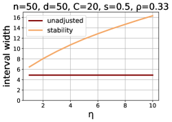
Refer to caption Refer to caption Refer to caption

Refer to caption Refer to caption Refer to caption

Refer to caption Refer to caption Refer to caption

Figure 12: Plots of average confidence interval widths of stable LASSO, with varying dimension and signal strength, in the Gaussian design case.

Refer to caption Refer to caption Refer to caption

Figure 13: Plots of average confidence interval widths of stable LASSO, with varying sample size, in the Gaussian design case.

A.13 Proof of Proposition 5 (marginal screening utility)

Fix s>0𝑠0s>0. Taking a union bound, we get:

{maxj[k]|cmj||cij|s|y}j=1k{|cmj||cij|s|y}.\mathbb{P}\!\left\{{\max_{j\in[k]}|c_{m_{j}}|-|c_{i_{j}}|\geq s}\ \middle|\ {y}\right\}\leq\sum_{j=1}^{k}\mathbb{P}\!\left\{{|c_{m_{j}}|-|c_{i_{j}}|\geq s}\ \middle|\ {y}\right\}.

At the time when ijsubscript𝑖𝑗i_{j} is chosen, exactly j1𝑗1j-1 items have been selected; therefore, at least one of m1,,mjsubscript𝑚1subscript𝑚𝑗m_{1},\dots,m_{j} has still not been selected. The event that |cmj||cij|ssubscript𝑐subscript𝑚𝑗subscript𝑐subscript𝑖𝑗𝑠|c_{m_{j}}|-|c_{i_{j}}|\geq s implies that ijsubscript𝑖𝑗i_{j} “beat” one of m1,,mjsubscript𝑚1subscript𝑚𝑗m_{1},\dots,m_{j}, which further implies that maxi[d]|ξj,i|s2subscript𝑖delimited-[]𝑑subscript𝜉𝑗𝑖𝑠2\max_{i\in[d]}|\xi_{j,i}|\geq\frac{s}{2}. By a union bound, this happens with probability at most dexp(snη/(4tr,1δ/(2d)X2,))𝑑𝑠𝑛𝜂4subscript𝑡𝑟1𝛿2𝑑subscriptnorm𝑋2d\exp(-sn\eta/(4t_{r,1-\delta/(2d)}\|X\|_{2,\infty})). Putting everything together, we get

j=1k{|cmj||cij|s|y}kdexp(snη4tr,1δ/(2d)X2,).\sum_{j=1}^{k}\mathbb{P}\!\left\{{|c_{m_{j}}|-|c_{i_{j}}|\geq s}\ \middle|\ {y}\right\}\leq kd\exp\left(-\frac{sn\eta}{4t_{r,1-\delta/(2d)}\|X\|_{2,\infty}}\right).

Plugging in s=4tr,1δ/(2d)log(dk/δ)X2,nη𝑠4subscript𝑡𝑟1𝛿2𝑑𝑑𝑘superscript𝛿subscriptnorm𝑋2𝑛𝜂s=\frac{4t_{r,1-\delta/(2d)}\log(dk/\delta^{\prime})\|X\|_{2,\infty}}{n\eta} completes the proof.

Refer to caption Refer to caption Refer to caption

Refer to caption Refer to caption Refer to caption

Refer to caption Refer to caption Refer to caption

Figure 14: Plots of average confidence interval widths of stable marginal screening and exact marginal screening with a conditional correction, with varying dimension and signal strength, in the Gaussian design case. We also plot the 90%percent9090\% quantile of the conditional width because it varies greatly across realizations.

Refer to caption Refer to caption Refer to caption

Figure 15: Plots of average confidence interval widths of stable marginal screening and exact marginal screening with a conditional correction, with varying sample size, in the Gaussian design case. In addition, we plot the 90%percent9090\% quantile of the conditional width because it varies greatly across realizations.

Appendix B Deferred numerical results and simulation details

Deferred plots.

We include plots of confidence interval widths, which were deferred from Section 9.

For the Gaussian design case, in Figure 12 we plot the widths corresponding to the experiments in Figure 4; in Figure 13 we plot the widths corresponding to the experiments in Figure 5; in Figure 14 we plot the widths corresponding to the experiments in Figure 6; in Figure 15 we plot the widths corresponding to the experiments in Figure 7.

For the Bernoulli design case, in Figure 16 we plot the widths corresponding to the experiments in Figure 8; in Figure 17 we plot the widths corresponding to the experiments in Figure 9; in Figure 18 we plot the widths corresponding to the experiments in Figure 10; in Figure 19 we plot the widths corresponding to the experiments in Figure 11. In Figure 18 and Figure 19, since the conditional widths are of a higher order of magnitude, the scale on the y𝑦y-axis in the widths plots is logarithmic.
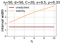
Refer to caption Refer to caption Refer to caption

Refer to caption Refer to caption Refer to caption

Refer to caption Refer to caption Refer to caption

Figure 16: Plots of average confidence interval widths of stable LASSO, with varying dimension and signal strength, in the Bernoulli design case.

Refer to caption Refer to caption Refer to caption

Figure 17: Plots of average confidence interval widths of stable LASSO, with varying sample size, in the Bernoulli design case.

Refer to caption Refer to caption Refer to caption

Refer to caption Refer to caption Refer to caption

Refer to caption Refer to caption Refer to caption

Figure 18: Plots of average confidence interval widths of stable marginal screening and exact marginal screening with a conditional correction, with varying dimension and signal strength, in the Bernoulli design case. We also plot the 90%percent9090\% quantile of the conditional width because it varies greatly across realizations.

Refer to caption Refer to caption Refer to caption

Figure 19: Plots of average confidence interval widths of stable marginal screening and exact marginal screening with a conditional correction, with varying sample size, in the Bernoulli design case. We also plot the 90%percent9090\% quantile of the conditional width because it varies greatly across realizations.

Experiments with Laplace errors.

We include additional experiments when the errors have an exponential, rather than Gaussian, tail: the outcome is generated as y=Xβ+ϵ𝑦𝑋𝛽italic-ϵy=X\beta+\leavevmode\nobreak\ \epsilon, where ϵii.i.d.Lap(12),i[n]\epsilon_{i}\stackrel{{\scriptstyle\mathrm{i.i.d.}}}{{\sim}}\mathrm{Lap}\left(\frac{1}{\sqrt{2}}\right),i\in[n]. The Laplace parameter is chosen so that the errors have variance equal to one.

For the Gaussian design case, Figure 20 shows plots analogous to those in Figure 4 and Figure 5 in this setting, and Figure 21 is the analogue of Figure 6 and Figure 7. Similarly, for the Bernoulli design case, Figure 22 is analogous to Figure 8 and Figure 9, and Figure 23 is analogous to Figure 10 and Figure 11.
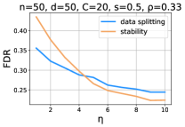
Refer to caption Refer to caption Refer to caption Refer to caption

Refer to caption Refer to caption Refer to caption Refer to caption

Refer to caption Refer to caption Refer to caption Refer to caption

Figure 20: Comparison of FDR after stable LASSO and LASSO with data splitting, with varying dimension and signal strength (first three columns) and sample size (last column), in the Gaussian design case. The errors are sampled from a Laplace distribution.
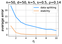
Refer to caption Refer to caption Refer to caption Refer to caption

Refer to caption Refer to caption Refer to caption Refer to caption

Refer to caption Refer to caption Refer to caption Refer to caption

Figure 21: Comparison of average error after stable marginal screening and marginal screening with data splitting, with varying dimension and signal strength (first three columns) and sample size (last column), in the Gaussian design case. The errors are sampled from a Laplace distribution.

Refer to caption Refer to caption Refer to caption Refer to caption

Refer to caption Refer to caption Refer to caption Refer to caption

Refer to caption Refer to caption Refer to caption Refer to caption

Figure 22: Comparison of FDR after stable LASSO and LASSO with data splitting, with varying dimension and signal strength (first three columns) and sample size (last column), in the Bernoulli design case. The errors are sampled from a Laplace distribution.

Refer to caption Refer to caption Refer to caption Refer to caption

Refer to caption Refer to caption Refer to caption Refer to caption

Refer to caption Refer to caption Refer to caption Refer to caption

Figure 23: Comparison of FDR after stable marginal screening and marginal screening with data splitting, with varying dimension and signal strength (first three columns) and sample size (last column), in the Bernoulli design case. The errors are sampled from a Laplace distribution.

Simulation details.

All plots of FDR and average error are averaged over 100001000010000 trials. Width plots are averaged over 500500500 trials because the stability correction implies interval widths of low variability. In each trial we generate a new triplet (X,β,y)𝑋𝛽𝑦(X,\beta,y), and run stable LASSO (respectively, marginal screening) on this data for all η𝜂\eta, as well as LASSO (respectively, marginal screening) with data splitting. For both stability and data splitting we take a Bonferroni correction to provide simultaneous coverage over all selected variables. Moreover, we note that η𝜂\eta in the plots refers to the noise parameter in Algorithm 2 and Algorithm 3; the actual stability parameter used to compute the corresponding splitting fraction for data splitting is multiplied by the number of steps of composition, i.e. we use f(kη)𝑓𝑘𝜂f(k\eta) as the splitting fraction. Finally, the δ𝛿\delta parameter in Algorithm 2 and Algorithm 3 is set to δ=0.5𝛿0.5\delta=0.5 throughout.

Appendix C Generalizations of stable algorithms

We show how our stable algorithms can be generalized beyond the setting of Gaussianity. Our proofs exploited Gaussianity of the outcome vector only in terms of the decay of its tails. In general we only need to know how tightly y𝑦y concentrates around μ𝜇\mu in order to reproduce the stable versions of the LASSO and marginal screening. To show this, we generalize our approach to all outcome vectors with bounded Orlicz norm. This includes other important cases such as general subgaussian and subexponential vectors y𝑦y.

Definition 3 (Orlicz norm).

A function ψ:00:𝜓subscript0subscript0\psi:\mathbb{R}_{\geq}0\rightarrow\mathbb{R}_{\geq}0 is an Orlicz function if ψ𝜓\psi is convex, non-decreasing, and satisfies ψ(0)=0𝜓00\psi(0)=0, ψ(x)𝜓𝑥\psi(x)\rightarrow\infty as x𝑥x\rightarrow\infty. For an Orlicz function ψ𝜓\psi, the Orlicz norm or ψ𝜓\psi-norm of a random variable W𝑊W is defined as

Wψ=inf{s>0:𝔼[ψ(|W|s)]1}.subscriptnorm𝑊𝜓infimumconditional-set𝑠0𝔼delimited-[]𝜓𝑊𝑠1\|W\|_{\psi}=\inf\left\{s>0:\mathbb{E}\left[\psi\left(\frac{|W|}{s}\right)\right]\leq 1\right\}.

This definition immediately implies a tail bound by Markov’s inequality:

{|W|sWψ}{ψ(|W|Wψ)ψ(s)}𝔼[ψ(|W|Wψ)]ψ(s)1ψ(s).𝑊𝑠subscriptnorm𝑊𝜓𝜓𝑊subscriptnorm𝑊𝜓𝜓𝑠𝔼delimited-[]𝜓𝑊subscriptnorm𝑊𝜓𝜓𝑠1𝜓𝑠\mathbb{P}\!\left\{{|W|\geq s\|W\|_{\psi}}\right\}\leq\mathbb{P}\!\left\{{\psi\left(\frac{|W|}{\|W\|_{\psi}}\right)\geq\psi(s)}\right\}\leq\frac{\mathbb{E}\left[\psi\left(\frac{|W|}{\|W\|_{\psi}}\right)\right]}{\psi(s)}\leq\frac{1}{\psi(s)}. (8)

A natural extension of Definition 3 to random vectors is to consider all one-dimensional projections.

Definition 4 (Orlicz norm in nsuperscript𝑛\mathbb{R}^{n}).

For a random vector Wn𝑊superscript𝑛W\in\mathbb{R}^{n} and Orlicz function ψ𝜓\psi, we define the Orlicz norm of W𝑊W as

Wψ=inf{s>0:supvn:v21Wvψs}.subscriptnorm𝑊𝜓infimumconditional-set𝑠0subscriptsupremum:𝑣superscript𝑛subscriptnorm𝑣21subscriptnormsuperscript𝑊top𝑣𝜓𝑠\|W\|_{\psi}=\inf\left\{s>0:\sup_{v\in\mathbb{R}^{n}:\|v\|_{2}\leq 1}\|W^{\top}v\|_{\psi}\leq s\right\}.

We state a corollary of Theorem 2, where we construct confidence intervals for stable selection methods as long as the outcomes have bounded ψ𝜓\psi-norm, for some Orlicz function ψ𝜓\psi.

Corollary 3.

Suppose yμψGsubscriptnorm𝑦𝜇𝜓𝐺\|y-\mu\|_{\psi}\leq G, for some known G>0𝐺0G>0, and fix δ(0,1)𝛿01\delta\in(0,1). Let M^^𝑀\hat{M} be an (η,τ,ν)𝜂𝜏𝜈(\eta,\tau,\nu)-stable model selection algorithm. For all jM^𝑗^𝑀j\in\hat{M}, let

CIjM^=(β^jM^±ψ1(|M^|eη/δ)G((XM^XM^)1)jj).subscriptCI𝑗^𝑀plus-or-minussubscript^𝛽𝑗^𝑀superscript𝜓1^𝑀superscript𝑒𝜂𝛿𝐺subscriptsuperscriptsuperscriptsubscript𝑋^𝑀topsubscript𝑋^𝑀1𝑗𝑗\mathrm{CI}_{j\cdot\hat{M}}=\left(\hat{\beta}_{j\cdot\hat{M}}\pm\psi^{-1}\left(|\hat{M}|e^{\eta}/\delta\right)G\sqrt{((X_{\hat{M}}^{\top}X_{\hat{M}})^{-1})_{jj}}\right).

Then

{jM^:βjMCIjM^}δ+τ+ν.conditional-set𝑗^𝑀subscript𝛽𝑗𝑀subscriptCI𝑗^𝑀𝛿𝜏𝜈\mathbb{P}\!\left\{{\exists j\in\hat{M}\leavevmode\nobreak\ :\leavevmode\nobreak\ \beta_{j\cdot M}\not\in\mathrm{CI}_{j\cdot\hat{M}}}\right\}\leq\delta+\tau+\nu.
Proof.

Fix a model M𝑀M. We only need to argue that

{maxjM|β^jMβjMG((XM^XM^)1)jj|ψ1(|M|eη/δ)}δeη.subscript𝑗𝑀subscript^𝛽𝑗𝑀subscript𝛽𝑗𝑀𝐺subscriptsuperscriptsuperscriptsubscript𝑋^𝑀topsubscript𝑋^𝑀1𝑗𝑗superscript𝜓1𝑀superscript𝑒𝜂𝛿𝛿superscript𝑒𝜂\mathbb{P}\!\left\{{\max_{j\in M}\left|\frac{\hat{\beta}_{j\cdot M}-\beta_{j\cdot M}}{G\sqrt{((X_{\hat{M}}^{\top}X_{\hat{M}})^{-1})_{jj}}}\right|\geq\psi^{-1}\left(|M|e^{\eta}/\delta\right)}\right\}\leq\delta e^{-\eta}.

Invoking Theorem 2 then completes the proof.

Denote by XjMsubscript𝑋𝑗𝑀X_{j\cdot M} the residual vector when Xjsubscript𝑋𝑗X_{j} is regressed onto all other variables in M𝑀M; that is, XjM=PXMjXjsubscript𝑋𝑗𝑀subscriptsuperscript𝑃perpendicular-tosubscript𝑋𝑀𝑗subscript𝑋𝑗X_{j\cdot M}=P^{\perp}_{X_{M\setminus j}}X_{j}, where PXMjsubscriptsuperscript𝑃perpendicular-tosubscript𝑋𝑀𝑗P^{\perp}_{X_{M\setminus j}} denotes the projection matrix onto the orthocomplement of XMjsubscript𝑋𝑀𝑗X_{M\setminus j}. With this notation, we can express the least-squares solution as

β^jM=XjMyXjM22,βjM=XjMμXjM22.formulae-sequencesubscript^𝛽𝑗𝑀superscriptsubscript𝑋𝑗𝑀top𝑦superscriptsubscriptnormsubscript𝑋𝑗𝑀22subscript𝛽𝑗𝑀superscriptsubscript𝑋𝑗𝑀top𝜇superscriptsubscriptnormsubscript𝑋𝑗𝑀22\hat{\beta}_{j\cdot M}=\frac{X_{j\cdot M}^{\top}y}{\|X_{j\cdot M}\|_{2}^{2}},\leavevmode\nobreak\ \leavevmode\nobreak\ \beta_{j\cdot M}=\frac{X_{j\cdot M}^{\top}\mu}{\|X_{j\cdot M}\|_{2}^{2}}.

Moreover, (XMXM)jj1=1XjM22subscriptsuperscriptsuperscriptsubscript𝑋𝑀topsubscript𝑋𝑀1𝑗𝑗1superscriptsubscriptnormsubscript𝑋𝑗𝑀22(X_{M}^{\top}X_{M})^{-1}_{jj}=\frac{1}{\|X_{j\cdot M}\|_{2}^{2}}. Using this fact, we have

{maxjM|β^jMβjMG((XM^XM^)1)jj|ψ1(|M|eη/δ)}subscript𝑗𝑀subscript^𝛽𝑗𝑀subscript𝛽𝑗𝑀𝐺subscriptsuperscriptsuperscriptsubscript𝑋^𝑀topsubscript𝑋^𝑀1𝑗𝑗superscript𝜓1𝑀superscript𝑒𝜂𝛿\displaystyle\mathbb{P}\!\left\{{\max_{j\in M}\left|\frac{\hat{\beta}_{j\cdot M}-\beta_{j\cdot M}}{G\sqrt{((X_{\hat{M}}^{\top}X_{\hat{M}})^{-1})_{jj}}}\right|\geq\psi^{-1}\left(|M|e^{\eta}/\delta\right)}\right\}
={maxjM|vjM(yμ)|Gψ1(|M|eη/δ)},absentsubscript𝑗𝑀superscriptsubscript𝑣𝑗𝑀top𝑦𝜇𝐺superscript𝜓1𝑀superscript𝑒𝜂𝛿\displaystyle=\mathbb{P}\!\left\{{\max_{j\in M}|v_{j\cdot M}^{\top}(y-\mu)|\geq G\psi^{-1}\left(|M|e^{\eta}/\delta\right)}\right\},

where we define vjMsubscript𝑣𝑗𝑀v_{j\cdot M} to be the random unit vector XjMXjM2subscript𝑋𝑗𝑀subscriptnormsubscript𝑋𝑗𝑀2\frac{X_{j\cdot M}}{\|X_{j\cdot M}\|_{2}}. By applying the tail bound given by Eq. (8) together with a union bound, we get

{maxjM|vjM(yμ)|Gψ1(|M|eη/δ)}subscript𝑗𝑀superscriptsubscript𝑣𝑗𝑀top𝑦𝜇𝐺superscript𝜓1𝑀superscript𝑒𝜂𝛿\displaystyle\mathbb{P}\!\left\{{\max_{j\in M}|v_{j\cdot M}^{\top}(y-\mu)|\geq G\psi^{-1}\left(|M|e^{\eta}/\delta\right)}\right\} jM{|vjM(yμ)|ψ1(|M|eη/δ)}absentsubscript𝑗𝑀superscriptsubscript𝑣𝑗𝑀top𝑦𝜇superscript𝜓1𝑀superscript𝑒𝜂𝛿\displaystyle\leq\sum_{j\in M}\mathbb{P}\!\left\{{|v_{j\cdot M}^{\top}(y-\mu)|\geq\psi^{-1}\left(|M|e^{\eta}/\delta\right)}\right\}
|M|(ψ(ψ1(|M|eη/δ)))1absent𝑀superscript𝜓superscript𝜓1𝑀superscript𝑒𝜂𝛿1\displaystyle\leq|M|\left(\psi\left(\psi^{-1}\left(|M|e^{\eta}/\delta\right)\right)\right)^{-1}
=δeη.absent𝛿superscript𝑒𝜂\displaystyle=\delta e^{-\eta}.

Now we can generalize the stable versions of the LASSO and marginal screening. We state counterparts of Algorithm 2 and Algorithm 3 which ensure stability as long as we know a bound G𝐺G on yμψsubscriptnorm𝑦𝜇𝜓\|y-\mu\|_{\psi}.

input: design matrix Xn×d𝑋superscript𝑛𝑑X\in\mathbb{R}^{n\times d}, outcome vector yn𝑦superscript𝑛y\in\mathbb{R}^{n}, 1subscript1\ell_{1}-constraint C1subscript𝐶1C_{1}, number of optimization steps k𝑘k, typical stability parameters δ(0,1),η>0formulae-sequence𝛿01𝜂0\delta\in(0,1),\eta>0

output: LASSO solution θ^LASSOdsubscript^𝜃LASSOsuperscript𝑑\hat{\theta}_{\mathrm{LASSO}}\in\mathbb{R}^{d}
Initialize θ1=0subscript𝜃10\theta_{1}=0
for t=1,2,,k𝑡12𝑘t=1,2,\dots,k do

        ϕC1{±ei}i=1dfor-allitalic-ϕsubscript𝐶1superscriptsubscriptplus-or-minussubscript𝑒𝑖𝑖1𝑑\forall\phi\in C_{1}\cdot\{\pm e_{i}\}_{i=1}^{d}, sample ξt,ϕi.i.d.Lap(4ψ1(1/δ)C1X2,Gnη)superscriptsimilar-toi.i.d.subscript𝜉𝑡italic-ϕLap4superscript𝜓11𝛿subscript𝐶1subscriptnorm𝑋2𝐺𝑛𝜂\xi_{t,\phi}\stackrel{{\scriptstyle\text{i.i.d.}}}{{\sim}}\text{Lap}\left(\frac{4\psi^{-1}(1/\delta)C_{1}\|X\|_{2,\infty}G}{n\eta}\right)
ϕC1{±ei}i=1dfor-allitalic-ϕsubscript𝐶1superscriptsubscriptplus-or-minussubscript𝑒𝑖𝑖1𝑑\forall\phi\in C_{1}\cdot\{\pm e_{i}\}_{i=1}^{d}, let αϕ=2nϕX(yXθt)+ξt,ϕsubscript𝛼italic-ϕ2𝑛superscriptitalic-ϕtopsuperscript𝑋top𝑦𝑋subscript𝜃𝑡subscript𝜉𝑡italic-ϕ\alpha_{\phi}=\frac{2}{n}\phi^{\top}X^{\top}(y-X\theta_{t})+\xi_{t,\phi}
Set ϕt=argminϕC1{±ei}i=1dαϕsubscriptitalic-ϕ𝑡subscriptargminitalic-ϕsubscript𝐶1superscriptsubscriptplus-or-minussubscript𝑒𝑖𝑖1𝑑subscript𝛼italic-ϕ\phi_{t}=\operatorname*{arg\,min}_{\phi\in C_{1}\cdot\{\pm e_{i}\}_{i=1}^{d}}\alpha_{\phi}
Set θt+1=(1Δt)θt+Δtϕtsubscript𝜃𝑡11subscriptΔ𝑡subscript𝜃𝑡subscriptΔ𝑡subscriptitalic-ϕ𝑡\theta_{t+1}=(1-\Delta_{t})\theta_{t}+\Delta_{t}\phi_{t}, where Δt=2t+2subscriptΔ𝑡2𝑡2\Delta_{t}=\frac{2}{t+2}
end for
Return θ^LASSO=θk+1subscript^𝜃LASSOsubscript𝜃𝑘1\hat{\theta}_{\mathrm{LASSO}}=\theta_{k+1}
Algorithm 6 Stable LASSO algorithm under general Orlicz norm ψ𝜓\psi

input: design matrix Xn×d𝑋superscript𝑛𝑑X\in\mathbb{R}^{n\times d}, outcome vector yn𝑦superscript𝑛y\in\mathbb{R}^{n}, model size k𝑘k

output: M^={i1,,ik}^𝑀subscript𝑖1subscript𝑖𝑘\hat{M}=\{i_{1},\dots,i_{k}\}
Compute (c1,,cd)=1nXydsubscript𝑐1subscript𝑐𝑑1𝑛superscript𝑋top𝑦superscript𝑑(c_{1},\dots,c_{d})=\frac{1}{n}X^{\top}y\in\mathbb{R}^{d}
res1=[d]subscriptres1delimited-[]𝑑\text{res}_{1}=[d]
for t=1,2,,k𝑡12𝑘t=1,2,\dots,k do

        iresifor-all𝑖subscriptres𝑖\forall i\in\text{res}_{i}, sample ξt,ii.i.d.Lap(2ψ1(1/δ)X2,Gnη)superscriptsimilar-toi.i.d.subscript𝜉𝑡𝑖Lap2superscript𝜓11𝛿subscriptnorm𝑋2𝐺𝑛𝜂\xi_{t,i}\stackrel{{\scriptstyle\text{i.i.d.}}}{{\sim}}\text{Lap}\left(\frac{2\psi^{-1}(1/\delta)\|X\|_{2,\infty}G}{n\eta}\right)
it=argmaxirest|ci+ξt,i|subscript𝑖𝑡subscriptargmax𝑖subscriptres𝑡subscript𝑐𝑖subscript𝜉𝑡𝑖i_{t}=\operatorname*{arg\,max}_{i\in\text{res}_{t}}|c_{i}+\xi_{t,i}|
rest+1=restitsubscriptres𝑡1subscriptres𝑡subscript𝑖𝑡\text{res}_{t+1}=\text{res}_{t}\setminus i_{t}
end for
Return M^={i1,,ik}^𝑀subscript𝑖1subscript𝑖𝑘\hat{M}=\{i_{1},\dots,i_{k}\}
Algorithm 7 Stable marginal screening algorithm under general Orlicz norm ψ𝜓\psi