Interstellar Extinction and Elemental Abundances
DRAFT:   

Abstract

Elements in the interstellar medium (ISM) exist in the form of gas or dust. The interstellar extinction and elemental abundances provide crucial constraints on the composition, size and quantity of interstellar dust. Most of the extinction modeling efforts have assumed the total (gas and dust) abundances of the dust-forming elements—known as the “interstellar abundances”, “interstellar reference abundances”, or “cosmic abundances”—to be solar and the gas-phase abundances to be environmentally independent. However, it remains unclear if the solar abundances are an appropriate representation of the interstellar abundances. Meanwhile, the gas-phase abundances are known to exhibit appreciable variations with local environments. Here we explore the viability of the abundances of B stars, the solar and protosolar abundances, and the protosolar abundances augmented by Galactic chemical enrichment (GCE) as an appropriate representation of the interstellar abundances by quantitatively examining the extinction and abundances of ten interstellar sightlines for which both the extinction curves and the gas-phase abundances of all the major dust-forming elements (i.e., C, O, Mg, Si and Fe) have been observationally determined. Instead of assuming a specific dust model and then fitting the observed extinction curves, for each sightline we apply the model-independent Kramers-Kronig relation, which relates the wavelength-integrated extinction to the total dust volume, to place a lower limit on the dust depletion. This, together with the observationally-derived gas-phase abundances, allows us to rule out the B-star, solar, and protosolar abundances as the interstellar reference standard and support the GCE-augmented protosolar abundances as a viable representation of the interstellar abundances.

1 Introduction

Elements in the interstellar medium (ISM) exist in the form of gas or dust. The interstellar gas-phase abundances of elements can be measured from their optical and ultraviolet (UV) spectroscopic absorption lines. The elements “missing” from the gas phase are bound up in dust grains, known as “interstellar depletion”. The dust-phase abundance of an element is derived by assuming a “reference abundance” and then from which subtracting off the gas-phase abundance. The reference abundance (also known as “interstellar abundance”, or “cosmic abundance”) of an element is the total abundance of this element (both in gas and in dust).

The interstellar abundances of heavy, dust-forming elements such as C, O, Mg, Si and Fe provide insight into the maximum amount of raw materials available for making the dust to account for the observed extinction, i.e., any dust models should not use more elements than what is available in the ISM. This involves two unknown (or not well determined) sets of abundances for the dust-forming elements: the interstellar reference abundances and the gas-phase abundances. Although it is well recognized that a viable dust model should satisfy the cosmic abundance constraints, what might be the most appropriate set of interstellar reference abundances and what are the true gas-phase abundances of the dust-forming elements have been subjects of much discussion in the past decades. Historically, the interstellar abundances are commonly assumed to be solar. The gas-phase abundances of C and O are often assumed to be invariable with respect to the local interstellar conditions (e.g., see Cardelli et al. 1996, Meyer et al. 1998) while Mg, Si and Fe appear to be fully depleted from the gas phase (i.e., their gas-phase abundances are negligible).

In the late 1990s, it was argued that, because of their young ages, the interstellar abundances might be better represented by those of B stars and young F, G stars which are “subsolar” (i.e., $\sim\,$60–70% of solar; Snow & Witt 1995, 1996, Sofia & Meyer 2001). However, if the interstellar abundances are indeed “subsolar”, the ISM seems to lack enough raw material to make the dust to account for the observed interstellar extinction (Li 2005). Meanwhile, the published solar abundances have undergone major changes over the years (see Table 1). The most recently determined solar abundances (Asplund et al. 2009; hereafter A09) are significantly reduced from their earlier values (e.g., Anders & Grevesse 1989). It is interesting to note that, using the non-local thermodynamic equilibrium (NLTE) techniques, Przybilla et al. (2008) and Nieva & Przybilla (2012) derived the photospheric abundances of heavy elements for unevolved early B-type stars. They found that the photospheric abundances of those B stars are in close agreement with the A09 solar abundances (see Table 1).

Lodders (2003) argued that the currently observed solar photospheric abundances (relative to H) must be lower than those of the proto-Sun because helium and other heavy elements have settled toward the solar interior since the time of its formation $\sim\,$4.55$\,{\rm Gyr}$ ago. Lodders (2003) further suggested that the protosolar abundances derived from the photospheric abundances by considering settling effects are more representative of the solar system abundances. With the settling effects taken into account, the A09 solar abundances are roughly consistent with the proto-Sun abundances of Lodders (2003). On the other hand, as the Galaxy evolves, heavy elements are expected to be enriched (Chiappini et al. 2003). Draine (2015) suggested that the protosolar abundances augmented by Galactic chemical enrichment (GCE) over the past 4.55 Gyrs might be the best estimate for the interstellar abundances in the solar neighborhood.

Regarding the gas-phase abundances of the dust-forming elements C, O, Mg, Si and Fe, numerous observational studies carried out in the past decade do not appear to favor a constant gas-phase C/H abundance of $\sim\,$140$\,{\rm ppm}$ (Cardelli et al. 1996) and a constant gas-phase O/H abundance of $\sim\,$320$\,{\rm ppm}$ (Meyer et al. 1998) which were commonly adopted by dust models. Also, contrary to what is commonly assumed by dust models, there seems to be nontrivial amounts of gas-phase Si, Mg and Fe (10% or more in many sight lines; Jensen et al. 2010).

Cardelli et al. (1996) determined the gas-phase C abundance to be $\left[{\rm C/H}\right]_{\rm gas}\approx 140\pm 20\,{\rm ppm}$ from the weak intersystem line of C II] at 2325$\,{\rm\AA}$ obtained with the Goddard High Resolution Spectrograph (GHRS) on board the Hubble Space Telescope (HST) for six sightlines which exhibit a wide range of extinction variation. They found that $\left[{\rm C/H}\right]_{\rm gas}$ shows no dependence on the physical condition of the gas (also see Sofia et al. 1997, 2004). However, for the 21 sightlines studied by Parvathi et al. (2012) and Sofia et al. (2011), $\left[{\rm C/H}\right]_{\rm gas}$ appears to decrease with $\langle n_{\rm H}\rangle$, the mean density of H. This was based on the strong 1334$\,{\rm\AA}$ C II absorption line obtained with HST/STIS. These sight lines include a variety of Galactic disk environments characterized by different extinction and sample paths ranging over three orders of magnitude in $\langle n_{\rm H}\rangle$.

Meyer et al. (1998) obtained high S/N ratio echelle spectra of the weak OI 1356$\,{\rm\AA}$ absorption of seven nearby diffuse clouds. They derived a mean abundance of $\left[{\rm O/H}\right]_{\rm gas}\approx 319\pm 14\,{\rm ppm}$ and found no statistically significant variations among the sight lines and no evidence of density-dependent O depletion. In contrast, using the Space Telescope Imaging Spectrograph (STIS) on board HST, Cartledge et al. (2001) performed high-resolution observations of the OI 1356$\,{\rm\AA}$ absorption of 11 translucent clouds and found an appreciably lower $\left[{\rm O/H}\right]_{\rm gas}$ which suggests a trend toward an enhanced O depletion for denser clouds. Jensen et al. (2005) analyzed the HST/STIS and HST/GHRS spectra of the OI 1356$\,{\rm\AA}$ absorption of 10 sight lines and found a trend of increasing O depletion with ${R_{V}}$ and $f({\rm H_{2}})$, the fraction of H in molecular form.

Based on the HST/STIS echelle spectra of the 1239, 1240$\,{\rm\AA}$ absorption of Mg II, Cartledge et al. (2006) determined $\left[{\rm Mg/H}\right]_{\rm gas}$, the gas-phase Mg abundance of 47 sight lines extending up to 6.5 kpc through the Galactic disk which probe a variety of interstellar environments, covering ranges of $\sim\,$4 orders of magnitude in $f({\rm H_{2}})$ and over two orders of magnitude in $\langle n_{\rm H}\rangle$. They found that the depletion of Mg is density-dependent.

Miller et al. (2007) determined the gas-phase Si and Fe abundances based on the HST/STIS data of the Si II] line at 2335$\,{\rm\AA}$ and the Fe II lines at 1142, 2234, 2249, 2260, and 2367$\,{\rm\AA}$ for six translucent clouds which sample a variety of extinction characteristics as indicated by their ${R_{V}}$ values, which range from 2.6 to 5.8. They found that $\left[{\rm Si/H}\right]_{\rm gas}$ and $\left[{\rm Fe/H}\right]_{\rm gas}$ vary from one sight line to another. Similarly, Haris et al. (2016) derived $\left[{\rm Si/H}\right]_{\rm gas}$ for 131 sight lines based on the HST/STIS, HST/GHRS and the International Ultraviolet Explorer (IUE) data and found that $\left[{\rm Si/H}\right]_{\rm gas}$ is correlated with $\langle n_{\rm H}\rangle$ and $f({\rm H_{2}})$.

The interstellar extinction and elemental abundances provide crucial constraints on the composition and size of interstellar dust. Practically, most of the extinction modeling efforts have been so far directed to the Galactic average extinction curve which is obtained by averaging over many clouds of different gas and dust properties (e.g., see Mathis et al. 1977, Draine & Lee 1984, Désert et al. 1990, Mathis 1996, Li & Greenberg 1997, Weingartner & Draine 2001, Zubko et al. 2004, Jones et al. 2013), despite the fact that the interstellar extinction curves actually exhibit considerable variations from one sightline to another. Also, most of the extinction modeling efforts have assumed a solar abundance and a constant gas-phase abundance for the dust-forming elements, even though as discussed above the interstellar reference abundance remains unknown and the gas-phase abundances exhibit appreciable variations with the local interstellar environments. Therefore, by modeling the Galactic average extinction curve, unavoidably, any details concerning the relationship between the dust properties and the physical and chemical conditions of the interstellar environments would have been lost.

In this work we will examine the extinction and elemental abundances of ten interstellar lines of sight for each of which both the extinction curve and the gas-phase abundances for all the major dust-forming elements C, O, Mg, Si and Fe have been observationally determined. Our goal is to investigate which would be the most appropriate set of interstellar reference abundances, those of B stars (Przybilla et al. 2008), solar (A09), protosolar (Lodders 2003), or protosolar+GCE (Draine 2015)? To reduce the number of model parameters, we will not model the extinction curves, instead, we will simply apply the model-independent Kramers-Kronig (KK) relation (Purcell 1969) to relate the wavelength-integrated extinction to the total dust volume. Then, for each assumed set of reference abundances, we will explore whether the remaining elements, after subtracting off their gas-phase abundances, are sufficient for accounting for the total dust volume derived from the KK relation. Our approach is essentially model-independent since it does not require the knowledge of the detailed optical properties and size distribution of the dust. All we need is a general assumption of the dust composition (e.g., silicate, graphite, oxides and iron).

This paper is organized as follows. We first compile in §2 a “gold” sample consisting of all the (10) sightlines for which the extinction curves from the near infrared (IR) to the far UV and the gas-phase abundances of C, O, Mg, Si, and Fe have been observationally determined. Based on the measured gas-phase abundances of the dust-forming elements and the adopted interstellar reference abundances, we derive in §3 for each line of sight the total dust volumes. We assume that interstellar dust is made of (i) graphite and iron-containing amorphous silicate, (ii) graphite and iron-lacking amorphous silicate plus iron oxides, or (iii) graphite and iron-lacking amorphous silicate plus iron. We then apply the KK relation to determine in §4 the wavelength-integrated extinction from the total dust volume. In §5 we compare the wavelength-integrated extinction derived from the KK relation with that derived from observations and find that only if the interstellar abundances are like the GCE-augmented protosolar abundances would the KK-based wavelength-integrated extinction exceed the observation-based wavelength-integrated extinction, which is implied by the KK relation. These results as well as the “missing O” problem and the relations between the extinction-to-gas ratios and the interstellar physical and chemical conditions of the lines of sight in this “gold” sample are also discussed in §5. Finally, we summarize our major results in §6.

2 The Sample

We first search for in the literature as many interstellar sightlines as possible for which both the extinction curves have been determined from the near-IR to the far-UV and the gas-phase abundances have been measured for all the major dust-forming elements C, O, Mg, Si, and Fe. To this end, we find ten such lines of sight and tabulate in Table 2 the gas-phase abundances of C, O, Mg, Si, and Fe as well as the column densities of atomic hydrogen $N({\rm HI})$, molecular hydrogen $N({\rm H_{2}})$ and the total hydrogen column densities $N_{\rm H}=N({\rm HI})+2N({\rm H_{2}})$. The extinction parameters $c_{1}^{\prime}$, $c_{2}^{\prime}$, $c_{3}^{\prime}$, $c_{4}^{\prime}$, $x_{\rm o}$ and $\gamma$ as well as ${A_{V}}$, $E(B-V)$ and ${R_{V}}$ are taken from Valencic et al. (2004) and tabulated in Table 3. These parameters characterize the UV extinction measured by the International Ultraviolet Explorer (IUE) at $3.3<\lambda^{-1}<8.7\,{\rm\mu m}^{-1}$ as a sum of three components: a linear background, a Drude profile for the 2175$\,{\rm\AA}$ extinction bump, and a far-UV nonlinear rise at $\lambda^{-1}>5.9\,{\rm\mu m}^{-1}$:

$$A_{\lambda}/A_{V}=c_{1}^{\prime}+c_{2}^{\prime}\,x+c_{3}^{\prime}\,D(x,\gamma,x_{\rm o})+c_{4}^{\prime}\,F(x)~{}~{}~{},$$ (1)

$$D(x,\gamma,x_{\rm o})=\frac{x^{2}}{\left(x^{2}-x_{\rm o}^{2}\right)^{2}+x^{2}\gamma^{2}}~{}~{}~{},$$ (2)

$$F(x)=\left\{\begin{array}[]{lr}0~{},&x<5.9\,{\rm\mu m}^{-1}~{}~{}~{},\\ 0.5392\,\left(x-5.9\right)^{2}+0.05644\,\left(x-5.9\right)^{3}~{},&x\geq 5.9\,{\rm\mu m}^{-1}~{}~{}~{},\\ \end{array}\right.$$ (3)

where $A_{\lambda}$ is the extinction at wavelength $\lambda$, $x\equiv 1/\lambda$ is the inverse wavelength in $\mu$m^-1, $c_{1}^{\prime}$ and $c_{2}^{\prime}$ define the linear background, $c_{3}^{\prime}$ defines the strength of the 2175$\,{\rm\AA}$ extinction bump which is approximated by $D(x,\gamma,x_{\rm o})$, a Drude function which peaks at $x_{\rm o}\approx 4.6\,{\rm\mu m}^{-1}$ and has a FWHM of $\gamma$, and $c_{4}^{\prime}$ defines the nonlinear far-UV rise. In the following, we will refer to the parametrization described by Equations (1–3) as the FM parametrization.

For each line of sight, we aim at integrating the extinction over wavelength from 0 to $\infty$ (i.e., $\int_{0}^{\infty}A_{\lambda}\,d\lambda$). For practical reasons, this is not possible since the extinction curve is observationally determined only over a limited wavelength range, usually from the near-IR to the far-UV. We shall therefore “construct”, for each sightline, the extinction curve from 912$\,{\rm\AA}$ to 1$\,{\rm cm}$ and then obtain

$$A_{\rm int}^{\rm obs}\equiv\int_{\rm 912\,{\rm\AA}}^{1\,{\rm cm}}A_{\lambda}\,d\lambda~{}~{}.$$ (6)

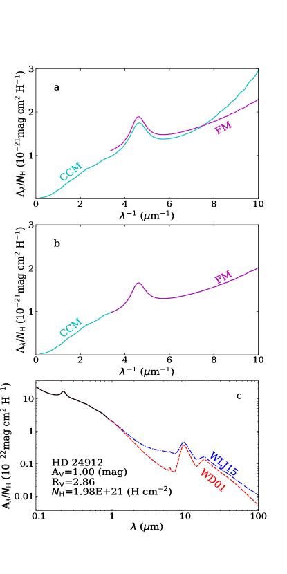
Figure 1: Constructing the interstellar extinction curve from the far-UV to the far-IR for the line of sight toward HD 24912. Panel (a): Comparison of the FM extinction curve at $\lambda^{-1}>3.3\,{\rm\mu m}^{-1}$ (purple line) and the CCM curve from the near-IR to far-UV (cyan line). The FM curve represents the observed IUE extinction curve, while the CCM curve is derived from the CCM parameterization with ${R_{V}}=2.86$ for HD 24912. Panel (b): The FM curve is multiplied by a factor to smoothly join the CCM curve at $\lambda^{-1}=3.3\,{\rm\mu m}^{-1}$. Panel (c): The interstellar extinction curve from the far-UV to the far-IR, with the FM curve for $\lambda^{-1}>3.3\,{\rm\mu m}^{-1}$, the CCM curve for $1.1\,{\rm\mu m}^{-1}<\lambda^{-1}<3.3\,{\rm\mu m}^{-1}$, and the ${R_{V}}=3.1$ model curves of Weingartner & Draine (2001; red dashed line) and Wang, Li & Jiang (2015a; blue dot-dashed line) for $0.9\,{\rm\mu m}<\lambda<1\,{\rm cm}$.

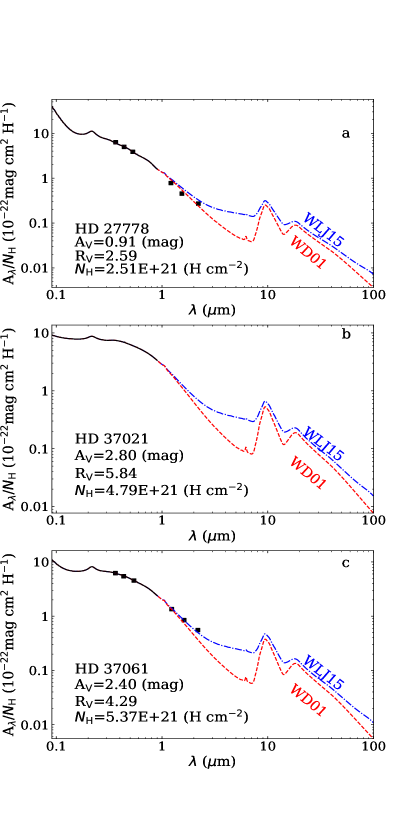
Figure 2: The interstellar extinction curves from the far-UV to the far-IR for the lines of sight toward HD 27778 (a), HD 37021 (b) and HD 37061 (c), with the FM curve for $\lambda^{-1}>3.3\,{\rm\mu m}^{-1}$, the CCM curve for $1.1\,{\rm\mu m}^{-1}<\lambda^{-1}<3.3\,{\rm\mu m}^{-1}$, and the ${R_{V}}=3.1$ model curves of Weingartner & Draine (2001; red dashed line) and Wang, Li & Jiang (2015a; blue dot-dashed line) for $0.9\,{\rm\mu m}<\lambda<1\,{\rm cm}$. Whenever available, broadband photometric extinction data (see Table 3) are shown as black squares. The U, B, V, J, H, K extinction data are superimposed on the extinction curves of HD 27778 (a) and HD 37061 (c).

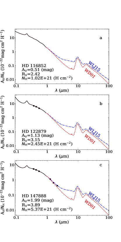
Figure 3: Same as Figure 2 but for HD 116852, HD 122879 and HD 147888. Black squares show the U, B, V extinction data for HD 122879 and the U, B, V, J, H, K extinction data for HD 147888.

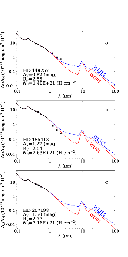
Figure 4: Same as Figure 2 but for HD 149757, HD 185418 and HD 207198. Black squares show the U, B, V, J, H, K extinction data for HD 149757 and HD 185418 and the U, B, V extinction data for HD 207198.

We construct the extinction curves as follows (see Figure 1). For $3.3<\lambda^{-1}<11\,{\rm\mu m}^{-1}$, we represent the extinction by Equation (1) with the extinction parameters taken from Table 3. For $1.1<\lambda^{-1}<3.3\,{\rm\mu m}^{-1}$, we compute the extinction from the parametrization of Cardelli et al. (1989; hereafter CCM). The CCM parametrization involves only one parameter, that this, ${R_{V}}$. As illustrated in Figure 1a, there is often a discontinuity between the FM parametrization at $\lambda^{-1}>3.3\,{\rm\mu m}^{-1}$ and the CCM parametrization at $\lambda^{-1}<3.3\,{\rm\mu m}^{-1}$. To comply with the observed extinction-to-gas ratio ${A_{V}}/N_{\rm H}$, we multiply the FM extinction curve by a factor to smoothly join the CCM curve (see Figure 1b). For $0.9\,{\rm\mu m}<\lambda<1\,{\rm cm}$, we approximate the extinction by the model extinction calculated from the standard silicate-graphite-PAH model of Weingartner & Draine (WD01) for ${R_{V}}=3.1$ (see Figure 1c). Note that the WD01 model extinction curve exhibits a deep minimum at $\sim\,$5–8$\,{\rm\mu m}$, whereas numerous observations made with the Infrared Space Observatory (ISO) and the Spitzer Space Telescope have shown that the mid-IR extinction at $3\,{\rm\mu m}<\lambda<8\,{\rm\mu m}$ is flat for both diffuse and dense environments (Lutz 1999, Indebetouw et al. 2005, Jiang et al. 2006, Flaherty et al. 2007, Gao et al. 2009, Nishiyama et al. 2009, Wang et al. 2013, Xue et al. 2016, Hensley & Draine 2020a). By introducing a population of very large, micron-sized graphitic grains, Wang et al. (2015a; hereafter WLJ15) closely reproduced the observed flat mid-IR extinction. Therefore, for $0.9\,{\rm\mu m}<\lambda<1\,{\rm cm}$, we will also approximate the extinction by the WLJ15 model extinction (see Figure 1c). As a result, for each sightline we derive two extinction curves (which we refer to as “WD01” and “WLJ15”; see Figures 2–4) and integrate the extinction (per hydrogen column) over 912$\,{\rm\AA}$ and 1$\,{\rm cm}$ to obtain $A_{\rm int}^{\rm obs}(\rm\scriptsize WD)/N_{\rm H}$ and $A_{\rm int}^{\rm obs}(\rm\scriptsize WLJ)/N_{\rm H}$. We have also tried our best to compile for each line of sight the broadband photometric extinction data (see Table 3). Whenever available, they are displayed as black squares superimposed on the synthesized extinction curves. As shown in Figures 2–4, the synthesized extinction curves of all lines of sight closely agree with the observationally-determined U, B and V extinction. While the WD01 curve of HD 27778 and the WLJ15 curves of HD 37061 and HD 147888 agree with their J, H, and K extinction data, the WD01 curve of HD 185418 is somewhat higher and the WLJ15 curve of HD 149757 is somewhat lower than their J, H, and K extinction data.

3 Total Dust Volumes as Constrained by the Elemental Abundances

For an assumed dust composition, for each line of sight we can estimate the total dust volume per H nucleon ($V_{\rm dust}$/H) from the adopted set of interstellar reference abundances and the observationally-determined gas-phase abundances. For the dust composition, we will first consider a mixture of amorphous silicate and graphite. It is well recognized that amorphous silicate is a ubiquitous component of the Universe as revealed by the 9.7$\,{\rm\mu m}$ Si–O stretching feature and the 18$\,{\rm\mu m}$ O–Si–O bending feature seen either in absorption or in emission (see Henning 2010). There must also be a population of carbon dust, although its exact composition remains unknown (see Henning & Salama 1998). This is because, as discussed in §1, C is partially depleted from the gas phase and silicate alone is not sufficient to account for the observed extinction (see Mishra & Li 2015, 2017). In this work we assume that all the C atoms missing from the gas phase are locked up in graphite grains since presolar graphite grains have been identified in primitive meteorites and the interstellar 2175$\,{\rm\AA}$ extinction bump, the strongest interstellar absorption feature, is generally attributed to small graphitic grains.

Let $\left[{\rm C/H}\right]_{\rm ISM}$ be the interstellar C abundance (relative to H). We calculate the volume per H nucleon ($V_{\rm gra}$/H) occupied by graphite dust from

$$\frac{V_{\rm gra}}{\rm H}=\left\{\left[{\rm C/H}\right]_{\rm ISM}-\left[{\rm C/H}\right]_{\rm gas}\right\}\frac{\mu_{\rm C}m_{\rm H}}{\rho_{\rm gra}}~{}~{},$$ (7)

where $\mu_{\rm C}=12$ is the atomic weight of C, $\rho_{\rm gra}\approx 2.2\,{\rm g}\,{\rm cm}^{-3}$ is the mass density of graphite, and $m_{\rm H}=1.66\times 10^{-24}\,{\rm g}$ is the mass of a hydrogen atom. For the silicate component, we assume an even mixture of pyroxene (Mg_xFe_1-xSiO₃) and olivine (Mg_2xFe_2-2xSiO₄) compositions, where $0\lesssim x\lesssim 1$. Therefore, we assign 3.5 O atoms for each Si atom. We calculate the volume per H nucleon ($V_{\rm sil}$/H) occupied by silicate dust from

$$\frac{V_{\rm sil}}{\rm H} =\Bigg{\{}\left(\left[{\rm Mg/H}\right]_{\rm ISM}-\left[{\rm Mg/H}\right]_{\rm gas}\right)\mu_{\rm Mg}+\left(\left[{\rm Fe/H}\right]_{\rm ISM}-\left[{\rm Fe/H}\right]_{\rm gas}\right)\mu_{\rm Fe}$$ (8)

$$+\left(\left[{\rm Si/H}\right]_{\rm ISM}-\left[{\rm Si/H}\right]_{\rm gas}\right)\mu_{\rm Si}+3.5\left(\left[{\rm Si/H}\right]_{\rm ISM}-\left[{\rm Si/H}\right]_{\rm gas}\right)\mu_{\rm O}\Bigg{\}}\frac{m_{\rm H}}{\rho_{\rm sil}}~{}~{},$$

where $\left[{\rm Mg/H}\right]_{\rm ISM}$, $\left[{\rm Fe/H}\right]_{\rm ISM}$, $\left[{\rm Si/H}\right]_{\rm ISM}$ and $\left[{\rm O/H}\right]_{\rm ISM}$ are respectively the interstellar Mg, Fe, Si and O abundances (relative to H), $\mu_{\rm Mg}$, $\mu_{\rm Fe}$, $\mu_{\rm Si}$ and $\mu_{\rm O}$ are respectively the atomic weights of Mg, Fe, Si and O, and $\rho_{\rm sil}\approx 3.5\,{\rm g}\,{\rm cm}^{-3}$ is the mass density of silicate dust.

We consider four sets of interstellar reference abundances, by adopting the abundances of B stars (Przybilla et al. 2008), solar abundances (A09), protosolar abundances (Lodders 2003), and GCE-augmented protosolar abundances (Draine 2015) as the interstellar abundances. For each adopted set of interstellar abundances, we calculate $V_{\rm gra}$/H and $V_{\rm sil}$/H from Equations (7,8) for each sightline and tabulate the results in Tables 4–7.

So far, we have assumed that all the Fe atoms missing from the gas phase are depleted in amorphous silicate grains. In the Galactic ISM, typically 90% or more of the Fe is missing from the gas phase (Jenkins 2009), suggesting that Fe is the largest elemental contributor to the interstellar dust mass after O and C and accounts for $\sim\,$25% of the dust mass in diffuse interstellar regions. However, as yet we know little about the nature of the Fe-containing material. Silicate grains provide a possible reservoir for the Fe in the form of interstellar pyroxene or olivine analogues. Nevertheless, iron abundances and depletions in the ISM often diverge from the pattern shown by Si and Mg, suggesting that Fe is not tied to the same grains as Si, and therefore most silicate grains are likely Mg-based. Also, the shape and strength of the interstellar 9.7$\,{\rm\mu m}$ silicate absorption feature suggest that the silicate material is Mg-rich rather than Fe-rich (Poteet et al. 2015) and hence a substantial fraction ($\sim\,$70%) of the interstellar Fe might be in other forms such as iron oxides, iron sulfides, or metallic iron (see Draine & Hensley 2013, Dwek 2016, Hensley & Draine 2017). Therefore, we will also consider the ISM to consist of graphite, Fe-lacking silicates (i.e., forsterite Mg₂SiO₄ and enstatite MgSiO₃), and three types of iron oxides (i.e., wüstite FeO, haematite Fe₂O₃, and magnetite Fe₃O₄). We assume that the Fe atoms missing from the gas phase are evenly tied up in FeO, Fe₂O₃, and Fe₃O₄. In this case, we calculate the volumes of silicate dust and iron oxides from

$$\frac{V_{\rm sil}}{\rm H} =\Bigg{\{}\left(\left[{\rm Mg/H}\right]_{\rm ISM}-\left[{\rm Mg/H}\right]_{\rm gas}\right)\mu_{\rm Mg}+\left(\left[{\rm Si/H}\right]_{\rm ISM}-\left[{\rm Si/H}\right]_{\rm gas}\right)\mu_{\rm Si}$$ (9)

$$+3.5\left(\left[{\rm Si/H}\right]_{\rm ISM}-\left[{\rm Si/H}\right]_{\rm gas}\right)\mu_{\rm O}\Bigg{\}}\frac{m_{\rm H}}{\rho_{\rm sil}^{\prime}}~{}~{},$$

$$\frac{V_{\rm FeO}}{\rm H} =\frac{1}{3}\Bigg{\{}\left(\left[{\rm Fe/H}\right]_{\rm ISM}-\left[{\rm Fe/H}\right]_{\rm gas}\right)\mu_{\rm Fe}+\left(\left[{\rm Fe/H}\right]_{\rm ISM}-\left[{\rm Fe/H}\right]_{\rm gas}\right)\mu_{\rm O}\Bigg{\}}\frac{m_{\rm H}}{\rho_{\rm FeO}}~{}~{},$$ (10)

$$\frac{V_{\rm Fe_{2}O_{3}}}{\rm H} =\frac{1}{3}\Bigg{\{}\left(\left[{\rm Fe/H}\right]_{\rm ISM}-\left[{\rm Fe/H}\right]_{\rm gas}\right)\mu_{\rm Fe}+\frac{3}{2}\left(\left[{\rm Fe/H}\right]_{\rm ISM}-\left[{\rm Fe/H}\right]_{\rm gas}\right)\mu_{\rm O}\Bigg{\}}\frac{m_{\rm H}}{\rho_{\rm Fe_{2}O_{3}}}~{}~{},$$ (11)

$$\frac{V_{\rm Fe_{3}O_{4}}}{\rm H} =\frac{1}{3}\Bigg{\{}\left(\left[{\rm Fe/H}\right]_{\rm ISM}-\left[{\rm Fe/H}\right]_{\rm gas}\right)\mu_{\rm Fe}+\frac{4}{3}\left(\left[{\rm Fe/H}\right]_{\rm ISM}-\left[{\rm Fe/H}\right]_{\rm gas}\right)\mu_{\rm O}\Bigg{\}}\frac{m_{\rm H}}{\rho_{\rm Fe_{3}O_{4}}}~{}~{},$$ (12)

where $\rho_{\rm sil}^{\prime}\approx 3.2\,{\rm g}\,{\rm cm}^{-3}$ is the mass density of Fe-lacking silicate, $\rho_{\rm FeO}\approx 5.7\,{\rm g}\,{\rm cm}^{-3}$, $\rho_{\rm Fe_{2}O_{3}}\approx 5.3\,{\rm g}\,{\rm cm}^{-3}$ and $\rho_{\rm Fe_{3}O_{4}}\approx 5.2\,{\rm g}\,{\rm cm}^{-3}$ are respectively the mass densities of FeO, Fe₂O₃ and Fe₃O₄ (see Table 8). Again, for each adopted set of interstellar abundances, we calculate $V_{\rm gra}$/H, $V_{\rm sil}$/H, $V_{\rm FeO}$, $V_{\rm Fe_{2}O_{3}}$ and $V_{\rm Fe_{3}O_{4}}$ from Equations (7, 9–12) for each sightline and tabulate the results in Tables 4–7.

Finally, we also consider the case of locking up all the Fe atoms missing from the gas phase in iron grains. In this case, the silicate dust volume is the same as Equation (9) and the volume of iron dust is

$$\frac{V_{\rm Fe}}{\rm H} =\Bigg{\{}\left(\left[{\rm Fe/H}\right]_{\rm ISM}-\left[{\rm Fe/H}\right]_{\rm gas}\right)\mu_{\rm Fe}\Bigg{\}}\frac{m_{\rm H}}{\rho_{\rm Fe}}~{}~{},$$ (13)

where $\rho_{\rm Fe}\approx 7.8\,{\rm g}\,{\rm cm}^{-3}$ is the mass density of iron. In Tables 4–7 we also tabulate $V_{\rm gra}$/H, $V_{\rm sil}$/H and $V_{\rm Fe}$/H calculated from Equations (7,9,13) respectively for four sets of interstellar reference abundances.

4 Total Wavelength-Integrated Extinction as Constrained by the Total Dust Volume

Let $A_{\rm int}^{\rm\scriptsize KK}\equiv\int_{0}^{\infty}A_{\lambda}\,d\lambda$ be the extinction integrated over all wavelengths. If, in the ISM, there are $N$ different types of dust species and $V_{j}$/H is the volume (per H nucleon) of the $j$-th dust type, the KK relation relates the wavelength-integrated extinction to the total volume (per H nucleon) occupied by dust through

$$A_{\rm int}^{\rm\scriptsize KK}/N_{\rm H}=\int_{0}^{\infty}A_{\lambda}/N_{\rm H}\,d\lambda=1.086\times 3\pi^{2}\sum_{j=1}^{N}F_{j}\,\left(V_{j}/{\rm H}\right)~{}~{},$$ (14)

where the dimensionless factor $F_{j}$ is the orientationally-averaged polarizability of the $j$-th dust type relative to the polarizability of an equal-volume sphere, depending only upon the grain shape and the static (zero-frequency) dielectric constant $\varepsilon_{0}$ of the grain material (Purcell 1969). In Table 8 we tabulate the $\varepsilon_{0}$ values for all the dust materials of interest in this work (i.e., graphite, iron, FeO, Fe₂O₃, Fe₃O₄, MgFeSiO₄, Mg₂SiO₄, and MgSiO₃).

To calculate the $F$ factors, we take the dust to be spheroids with semiaxes $a,b,b$ (prolate if $a/b>1$, oblate if $a/b<1$), then $F$ is related to the static dielectric constant $\varepsilon_{0}$ and the “depolarization factors” $L_{a}$ and $L_{b}=(1-L_{a})/2$ through

$$F(a/b,\varepsilon_{0})\equiv\frac{(\varepsilon_{0}-1)}{9}\left[\frac{1}{(\varepsilon_{0}-1)L_{a}+1}+\frac{2}{(\varepsilon_{0}-1)L_{b}+1}\right]~{}~{}~{},$$ (15)

where for prolates

$$L_{a}=\frac{1-e^{2}}{e^{2}}\left[\frac{1}{2e}\ln\left(\frac{1+e}{1-e}\right)-1\right]~{}~{}~{},$$ (16)

and for oblates

$$L_{a}=\frac{1+e^{2}}{e^{2}}\left[1-\frac{1}{e}\arctan(e)\right]~{}~{}~{},$$ (17)

where

$$e\equiv|1-(b/a)^{2}|^{1/2}~{}~{}~{}.$$ (18)

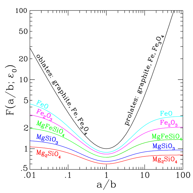
Figure 5: $F(\varepsilon_{0};{\rm shape})$ factors as a function of the axial ratio $a/b$ for Mg₂SiO₄ (red line), MgSiO₃ (blue line), MgFeSiO₄ (green line), FeO (cyan line), Fe₂O₃ (magenta line), as well as Fe, Fe₃O₄ and graphite (black line) of which the static dielectric constants are approximately $\varepsilon_{0}$ $\approx$ 5.5, 6.7, 10, 24,16, $\infty$, $\infty$ and $\infty$, respectively (Li 2005). The grains are taken to be spheroidal with $a$ and $b$ being the semiaxis along and perpendicular to the symmetry axis of the spheroid, respectively. The oblate dust is with axial $a/b<1$ while the prolate is with axial $a/b>1$. For modestly elongated ($a/b\lesssim 3$) or flattened ($b/a\lesssim 3$) silicate dust, the $\rm F$ factor is always smaller than unity.

By making use of the $\varepsilon_{0}$ values shown in Table 8, we calculate the $F$ factors as a function of grain shape (i.e., elongation $a/b$) for all the dust species considered here (see Figure 5). It is apparent that for both dielectric materials (e.g., MgFeSiO₄, Mg₂SiO₄, MgSiO₃, FeO, Fe₂O₃) and conducting materials (e.g., graphite, iron, Fe₃O₄), the $F$ factors of modestly elongated or flattened grains do not deviate much from unity. In this work, for each dust type we will adopt the mean $F$ value averaged over that calculated for $a/b=3$ prolates and $a/b=1/2$ oblates (see Table 8). The $a/b=3$ prolate shape is chosen because Greenberg & Li (1996) found that the 9.7 and 18$\,{\rm\mu m}$ silicate polarization toward the Becklin-Neugebauer (BN) object is best reproduced by $a/b=3$ core-mantle spheroids, while the $a/b=1/2$ oblate shape is selected because Lee & Draine (1985) found that the 3.1$\,{\rm\mu m}$ ice polarization of the BN object is best explained by $a/b=1/2$ oblates. Also, Hildebrand & Dragovan (1995) found that $a/b=1/2$ bare silicate oblates could fit the 9.7$\,{\rm\mu m}$ polarization of the BN object.

For each adopted set of interstellar reference abundances, depending on how the Fe atoms missing from the gas phase are divided among amorphous silicates, oxides and iron grains, we have accordingly calculated in §3 the possible total dust volumes for each line of sight (see Tables 4–7). Combining the dust volumes derived in §3 and the $F$ factors derived in this section, we calculate and tabulate in Tables 4–7 for each sightline $A_{\rm int}^{\rm\scriptsize KK}$, the extinction integrated over all wavelengths, for each of the four interstellar reference abundances (i.e., B-star, solar, protosolar, and GCE-augmented protosolar abundances) and each of three different dust mixtures (i.e., graphite + Fe-containg silicate, graphite + Fe-lacking silicate + iron oxides, and graphite + Fe-lacking silicate + Fe).

It is interesting to note that the $A_{\rm int}^{\rm\scriptsize KK}$ values calculated for different dust mixtures are rather close. Compared with the graphite + Fe-containg silicate mixture, the graphite + Fe-lacking silicate + iron oxides mixture contains more mass (on a per H nucleon basis). But the total dust volume of the latter exceeds that of the former by only several percent (because of the mass-density differences between Fe-containg silicates with iron oxides and Fe-lacking silicates). Although the $F$ factors of Fe-containing silicates are smaller than that of iron oxdies, they are larger than that of Fe-lacking silicates. Adding these effects together, the resulting $A_{\rm int}^{\rm\scriptsize KK}$ values of the graphite + Fe-lacking silicate + iron oxides mixture differ little from that of the graphite + Fe-containing silicate mixture. On the other hand, because of the higher mass density of iron (compared with silicates), the total dust volume of the graphite + Fe-lacking silicate + Fe mixture is smaller than that of the graphite + Fe-containg silicate mixture. The higher $F$ factor of iron does not sufficiently compensate the smaller dust volume and therefore the graphite + Fe-lacking silicate + Fe mixture actually has a lower $A_{\rm int}^{\rm\scriptsize KK}$ value than the graphite + Fe-containg silicate mixture.

The aforementioned results are derived from the KK-based wavelength-integrated extinction of Purcell (1969) who assumed nonmagnetic grains (see Equation [14]). For magnetic grains, incident electromagnetic waves certainly excite the oscillation of magnetic moments and result in the loss of the incident electromagnetic waves. Therefore, the absorption due to magnetic dipole moments from ferromagnetic (Fe) and ferrimagnetic (Fe₂O₃ and Fe₃O₄) grains could be appreciable and the wavelength integral of extinction becomes

$$\int_{0}^{\infty}A_{\lambda}/N_{\rm H}\,d\lambda=1.086\times 3\pi^{2}\sum_{j=1}^{N}\left\{F_{j}(a/b,\varepsilon_{0})+F_{j}(a/b,\mu_{0})\right\}\left(V_{j}/{\rm H}\right)~{}~{},$$ (19)

where the dimensionless factor $F(a/b,\varepsilon_{0})$, as defined in Equation (15), measures the electric response, while the dimensionless factor $F(a/b,\mu_{0})$ measures the magnetic response (see Draine & Lazarian 1999):

$$F(a/b,\mu_{0})\equiv\frac{(\mu_{0}-1)}{9}\left[\frac{1}{(\mu_{0}-1)L_{a}+1}+\frac{2}{(\mu_{0}-1)L_{b}+1}\right]~{}~{}~{},$$ (20)

where $\mu_{0}$ is the static (zero-frequency) magnetic permeability of the grain material (for nonmagnetic grains $\mu_{0}\approx 1$ and therefore $F(a/b,\mu_{0})\approx 0$). For grain materials having $\varepsilon_{0}\gtrsim 3$ and $\mu_{0}\gtrsim 3$, $F(a/b,\mu_{0})\approx F(a/b,\varepsilon_{0})$, and we see from Equations (14) and (19) that the wavelength integral of extinction for magnetic grains (e.g., Fe, Fe₂O₃ and Fe₃O₄) would be increased by a factor of $\left\{1+F(a/b,\mu_{0})/F(a/b,\varepsilon_{0})\right\}\approx 2$ than it would have been had the grains been nonmagnetic. However, as demonstrated in Draine & Lazarian (1999) and Draine & Hensley (2013), the magnetic dipole absorption mostly occurs at $\lambda\gtrsim 3\,{\rm mm}$ and its contribution to the extinction of interest here is not important since we are mostly concerned with the UV, optical, near- and mid-IR interstellar extinction. This justifies the neglect of the magnetic dipole absorption of magnetic grains (i.e., Fe, Fe₂O₃ and Fe₃O₄) in this work.

5 Results and Discussion

For a fixed amount of dust materials, $A_{\rm int}^{\rm\scriptsize KK}/N_{\rm H}$ gives the maximum possible amount of wavelength-integrated extinction per H nucleon (see Equation [14]), while both $A_{\rm int}^{\rm obs}(\rm\scriptsize WD)/N_{\rm H}$ and $A_{\rm int}^{\rm obs}(\rm\scriptsize WLJ)/N_{\rm H}$ are obtained by integrating the “observed” extinction over a finite wavelength range (see Equation [6]). For an interstellar reference abundance standard to be a viable representation of the “true” interstellar abundances, the amounts of dust-forming elements available for making dust have to be sufficient to account for the observed extinction. This implies that $A_{\rm int}^{\rm\scriptsize KK}/N_{\rm H}$ should exceed $A_{\rm int}^{\rm obs}(\rm\scriptsize WD)/N_{\rm H}$ and $A_{\rm int}^{\rm obs}(\rm\scriptsize WLJ)/N_{\rm H}$ since the extinction $A_{\lambda}/N_{\rm H}$ is always positive and therefore it is always true that $\int_{0}^{\infty}A_{\lambda}/N_{\rm H}\,d\lambda\,>\,\int_{912\,{\rm\AA}}^{1\,{\rm cm}}A_{\lambda}/N_{\rm H}\,d\lambda$. For an adopted set of interstellar reference abundances, if the corresponding $A_{\rm int}^{\rm\scriptsize KK}/N_{\rm H}$ is smaller than or equal to $A_{\rm int}^{\rm obs}(\rm\scriptsize WD)/N_{\rm H}$ and $A_{\rm int}^{\rm obs}(\rm\scriptsize WLJ)/N_{\rm H}$, it simply means that the adopted reference abundances are not viable since there would be insufficient amounts of dust-forming elements to make the dust to cause the observed amounts of extinction.

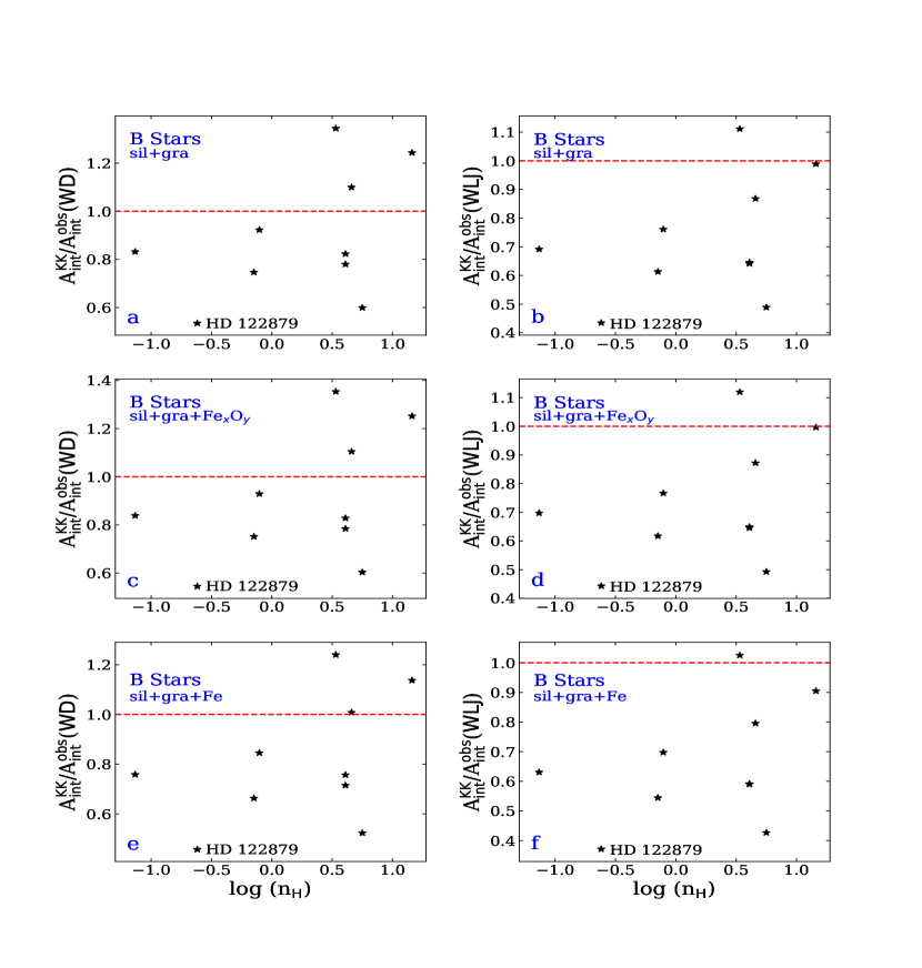
Figure 6: Comparison of the KK-based wavelength-integrated extinction $A_{\rm int}^{\rm\scriptsize KK}$ with the observation-based wavelength-integrated extinction $A_{\rm int}^{\rm obs}(\rm\scriptsize WD)$ and $A_{\rm int}^{\rm obs}(\rm\scriptsize WLJ)$ for the “gold” sample of 10 lines of sight, with $A_{\rm int}^{\rm\scriptsize KK}$ derived from the assumption of the abundances of B stars as the interstellar reference abundances and the dust as mixtures of (i) graphite and Fe-containing amorphous silicates (a, b), (ii) graphite and Fe-lacking amorphous silicates plus iron oxides (c, d), and (iii) graphite and Fe-lacking amorphous silicates plus iron (e, f). The observation-based wavelength-integrated extinction $A_{\rm int}^{\rm obs}(\rm\scriptsize WD)$ and $A_{\rm int}^{\rm obs}(\rm\scriptsize WLJ)$ are obtained by integrating the “observed” extinction curve from 912$\,{\rm\AA}$ to 1$\,{\rm cm}$, with the extinction curve at $0.9\,{\rm\mu m}<\lambda<1\,{\rm cm}$ respectively approximated by the ${R_{V}}=3.1$ model curve of Weingartner & Draine (2001) and of Wang, Li & Jiang (2015a). For the adopted interstellar reference standard to be viable, we require for all sightlines $A_{\rm int}^{\rm\scriptsize KK}/A_{\rm int}^{\rm obs}(\rm\scriptsize WD)>1$ and $A_{\rm int}^{\rm\scriptsize KK}/A_{\rm int}^{\rm obs}(\rm\scriptsize WLJ)>1$.

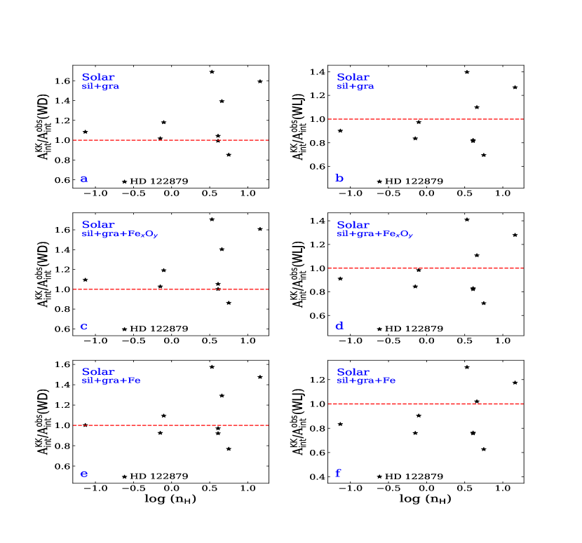
Figure 7: Same as Figure 6 but with the solar abundances as the interstellar reference abundances.

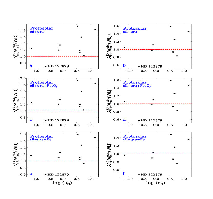
Figure 8: Same as Figure 6 but with the protosolar abundances as the interstellar reference abundances.

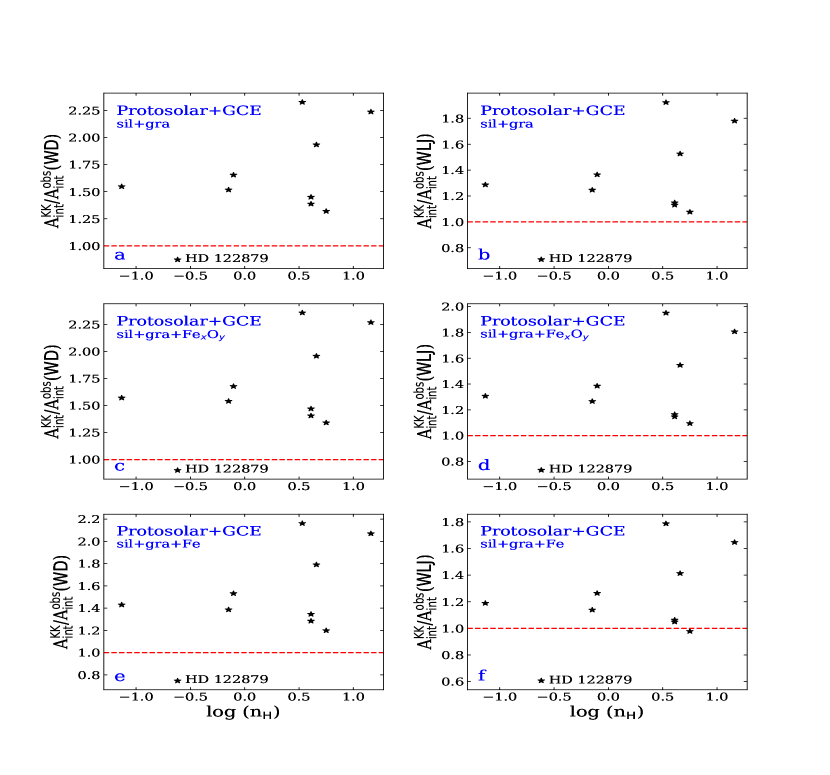
Figure 9: Same as Figure 6 but with the GCE-augmented protosolar abundances as the interstellar reference abundances.

We first consider the abundances of B stars. In Figure 6 we compare the wavelength-integrated “observed” extinction $A_{\rm int}^{\rm obs}(\rm\scriptsize WD)/N_{\rm H}$ and $A_{\rm int}^{\rm obs}(\rm\scriptsize WLJ)/N_{\rm H}$ with $A_{\rm int}^{\rm\scriptsize KK}/N_{\rm H}$, the KK-based extinction integrated over all wavelengths obtained by assuming the interstellar abundances are that of B stars. With $A_{\rm int}^{\rm\scriptsize KK}/N_{\rm H}$ exceeding $A_{\rm int}^{\rm obs}(\rm\scriptsize WLJ)/N_{\rm H}$ for only one sightline (over 10 sightlines), it is apparent that the B-star abundances are not a viable representation of the interstellar abundances. Even if we compare $A_{\rm int}^{\rm\scriptsize KK}/N_{\rm H}$ with $A_{\rm int}^{\rm obs}(\rm\scriptsize WD)/N_{\rm H}$, we still find $A_{\rm int}^{\rm\scriptsize KK}/N_{\rm H}<A_{\rm int}^{\rm obs}(\rm\scriptsize WD)/N_{\rm H}$ for the majority (7 over 10) of the sightlines. This is true, irrespective of the exact form which the Fe atoms missing from the gas phase take (i.e., amorphous silicates, iron oxides or solid iron). We have also considered the solar abundances as the interstellar reference abundances. As illustrated in Figure 7, we reach $A_{\rm int}^{\rm\scriptsize KK}/N_{\rm H}>A_{\rm int}^{\rm obs}(\rm\scriptsize WLJ)/N_{\rm H}$ only for a small fraction (3/10) of the sightlines. Even if we assume the interstellar abundances to be that of protosolar, the number of sightlines with $A_{\rm int}^{\rm\scriptsize KK}/N_{\rm H}<A_{\rm int}^{\rm obs}(\rm\scriptsize WLJ)/N_{\rm H}$ persists to be substantial. As shown in Figure 8, half of the 10 sightlines still have $A_{\rm int}^{\rm\scriptsize KK}/N_{\rm H}<A_{\rm int}^{\rm obs}(\rm\scriptsize WLJ)/N_{\rm H}$. However, this changes when the GCE-augmented protosolar abundances are adopted as the interstellar reference standard. As shown in Figure 9, we achieve $A_{\rm int}^{\rm\scriptsize KK}/N_{\rm H}>A_{\rm int}^{\rm obs}(\rm\scriptsize WLJ)/N_{\rm H}$ for all the sightlines except HD 122879. The line of sight toward HD 122879 has an unusually large gas-phase carbon abundance of $\left[{\rm C/H}\right]_{\rm gas}\approx 324\pm 38\,{\rm ppm}$ (Parvathi et al. 2012). Such a high $\left[{\rm C/H}\right]_{\rm gas}$ abundance is difficult to reconcile with the observed extinction and other C-related interstellar spectral phenomena. Therefore, we argue that the GCE-augmented protosolar abundances are a viable interstellar reference standard.

So far, we have assumed the carbonaceous dust component to be graphite. However, other forms of carbonaceous solid materials (e.g., amorphous carbon) have also been postulated to be a major interstellar dust component (see Henning & Salama 1998). Depending on their H contents, the mass densities of laboratory amorphous carbon materials range from $\sim\,$1.4$\,{\rm g}\,{\rm cm}^{-3}$ to $\sim\,$2.0$\,{\rm g}\,{\rm cm}^{-3}$ (see Jäger et al. 1998, Li & Greenberg 2002). On the other hand, those (H-rich) materials with a low mass density often have no or low DC conductivities (Jäger et al. 1998) and therefore their static dielectric constants $\varepsilon_{0}$ are much smaller than that of graphite. This implies a smaller $F$ factor than that of graphite for H-rich amorphous carbon. Although a lower mass density leads to a larger dust volume (see Equation [7]), this will be compensated by a smaller $F$ so that the KK-based wavelength-integrated $A_{\rm int}^{\rm\scriptsize KK}$ will not be appreciably affected (see Equation [14]). Even if we adopt the $F$ factor of graphite for amorphous carbon and assume a mass density of 1.8$\,{\rm g}\,{\rm cm}^{-3}$, the resulting $A_{\rm int}^{\rm\scriptsize KK}$ would only increase by $\sim\,$10% and this would not affect our conclusion.

We have so far also assumed that the ISM consists of separate, distinct individual grain populations (i.e., amorphous silicate, graphite, iron oxides, and iron). However, in the literature other dust structural forms have also been proposed, including silicate core-carbon mantle grains (Jones et al. 1990, Li & Greenberg 1997), composite grains consisting of small silicates, amorphous carbon, and vacuum (Mathis 1996), and composite “astrodust” consisting of amorphous silicates, metal oxides, hydrocarbons, and vaccum (Draine & Hensley 2020). Nevertheless, whether the dust takes a core-mantle structure or a mixture of separate, distinct individual grains would not affect the dust volume as long as the amount of dust material is fixed. On the other hand, compared to compact grains of the same amount of material, a larger volume is expected for composite grains. However, composite grains will have a smaller $F$ due to the reduction of their static dielectric constant $\varepsilon_{0}$ (see Li 2005) and hence are not expected to result in a higher $A_{\rm int}^{\rm\scriptsize KK}$. Therefore, what exact structural form interstellar dust may take does not affect our conclusion.

As early as mid-1990s, it has been recognized that, if the interstellar abundances are like that of B stars, the amount of C atoms left for dust after subtracting the gas-phase C abundance are insufficient to form the carbonaceous dust species required by dust models (Snow & Witt 1995, 1996). This, known as the “C crisis”, still holds even if one assumes the interstellar C abundance to be solar. For O, there is also a case of “O crisis” or “missing O”. Unlike C which is insufficient, for O there is as much as $\sim\,$160$\,{\rm ppm}$ of O/H unaccounted for in interstellar atoms, molecules and dust (Jenkins 2009, Whittet 2001a,b). Wang et al. (2015b) suggested that $\mu$m-sized H₂O ice grains could accommodate the excess O/H without exhibiting the 3.1$\,{\rm\mu m}$ absorption band of H₂O ice and they could be present in the diffuse ISM through rapid exchange of material between dense clouds where they form and diffuse clouds where they are destroyed by photosputtering. Alternatively, H₂O ice could be trapped in silicates. Very recently, Potapov et al. (2020) found evidence for the trapping of H₂O ice in silicate grains based on an analysis of the Spitzer/IRS spectra in combination with laboratory data. We examine the depletion of O in the context of the GCE-augmented protosolar abundances as the interstellar reference standard. If we assume that the ISM consists of graphite and Fe-containing silicates (or Fe-lacking silicates plus iron grains), the total amount of O/H which the ISM could accommodate is

$$\left[{\rm O/H}\right]_{\rm tot}\approx\left[{\rm O/H}\right]_{\rm gas}+3.5\times\left\{\left[{\rm Si/H}\right]_{\rm ISM}-\left[{\rm Si/H}\right]_{\rm gas}\right\}~{}~{}.$$ (21)

Similarly, if the ISM consists of graphite and Fe-lacking silicates plus iron oxides, the ISM could accommodate a total amount of

$$\left[{\rm O/H}\right]_{\rm tot}\approx\left[{\rm O/H}\right]_{\rm gas}+3.5\times\left\{\left[{\rm Si/H}\right]_{\rm ISM}-\left[{\rm Si/H}\right]_{\rm gas}\right\}+\frac{23}{18}\times\left\{\left[{\rm Fe/H}\right]_{\rm ISM}-\left[{\rm Fe/H}\right]_{\rm gas}\right\}~{}~{},$$ (22)

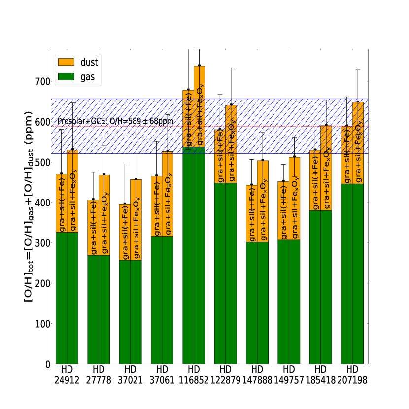
Figure 10: Comparison of the GCE-augmented protosolar O/H abundance (589$\pm$68$\,{\rm ppm}$; blue horizontal shaded box) with $\left[{\rm O/H}\right]_{\rm tot}$, the total amounts of O/H that could be accommodated by gas (green vertical boxes) and dust (orange vertical boxes) in each line of sight. The (vertical) error bars are for $\left[{\rm O/H}\right]_{\rm tot}$, resulting from the uncertainties in $\left[{\rm O/H}\right]_{\rm gas}$ and the uncertainties in the GCE-augmented protoslar Si/H and Fe/H abundances.

where we assume equal amounts of FeO, Fe₂O₃ and Fe₃O₄. Taking $\left[{\rm Si/H}\right]_{\rm ISM}$ and $\left[{\rm Fe/H}\right]_{\rm ISM}$ to be that of the GCE-augmented protosolar abundances, for each line of sight, we calculate $\left[{\rm O/H}\right]_{\rm tot}$ for different dust mixtures. In Figure 10 we compare $\left[{\rm O/H}\right]_{\rm tot}$ with the GCE-augmented protosolar O/H abundance. It appears that the majority of the sightlines have no difficulty in accommodating the “missing O”, particularly if the Fe atoms are tied up in oxides. Very recently, Psaradaki et al. (2020) compared the experimental X-ray spectra of the oxygen K edges of various silicate and oxide dust materials with the X-ray spectrum of Cygnus X-2, a bright low-mass X-ray binary, observed by XMM-Newton. They derived a remarkably high gas-phase abundance of $\left[{\rm O/H}\right]_{\rm gas}\approx 610\pm 60\,{\rm ppm}$ for the line of sight toward Cygnus X-2, although an accurate derivation of the $\left[{\rm O/H}\right]_{\rm gas}$ abundance relies on an accurate knowldge of the atomic data of the oxygen edge spectral region. Also, they determined the solid-phase O/H abundance to be $\left[{\rm O/H}\right]_{\rm dust}\approx 45\pm 7\,{\rm ppm}$, which is smaller than that could be accommodated by silicate dust alone by a factor of $\sim\,$3. Nevertheless, the total O/H abundance falls in the high side of the GCE-augmented protosolar O/H abundance.

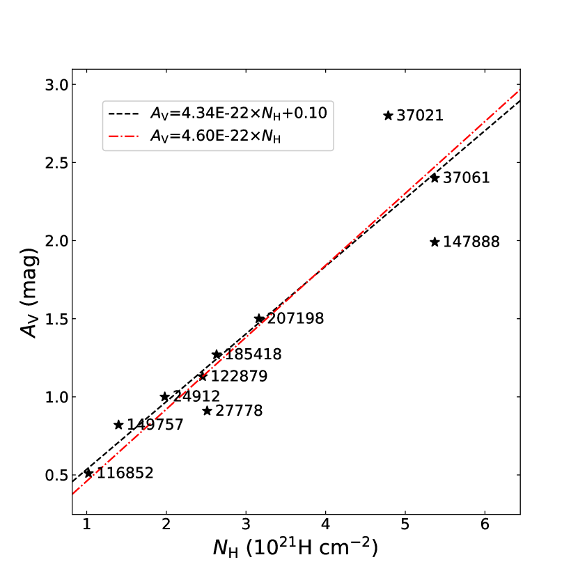
Figure 11: Visual extinction (${A_{V}}$) against the hydrogen column densities ($N_{\rm H}$) for the “gold” sample of 10 sightlines for which both the extinction parameters and the gas-phase abundances of C, O, Si, Mg and Fe have been observationally determined. Broken lines fit a linear relationship to the data. The goodness of fit is measured by $\chi^{2}/{\rm dof}$, the chi-square per degree of freedom ($\chi^{2}/{\rm dof}\approx 0.35$ for black dashed line and $\chi^{2}/{\rm dof}\approx 0.37$ for red dot-dashed line).

It is widely believed that in the ISM dust and gas are well mixed, as evidenced by the tight empirical correlation between reddening $E(B-V)$ and hydrogen column density $N_{\rm H}$. Bohlin et al. (1978) derived the hydrogen-to-reddening ratio to be $N_{\rm H}/E(B-V)\approx 5.8\times 10^{21}\,{\rm H}\,{\rm cm}^{-2}\,{\rm mag}^{-1}$ for a sample of 100 stars with $E(B-V)$ up to $\sim\,$0.5$\,{\rm mag}$, based on the UV absorption spectra of HI and H₂ observed by the Copernicus satellite. With ${R_{V}}\approx 3.1$ for the Galactic diffuse ISM, this corresponds to ${A_{V}}/N_{\rm H}\approx 5.3\times 10^{-22}\,{\rm mag}\,{\rm cm}^{2}\,{\rm H}^{-1}$, a ratio long taken to be representative of the ISM in the solar neighbourhood. However, appreciably lower extinction-to-hydrogen ratios have been reported (see Hensley & Draine [2020b] and references therein), e.g., Lenz et al. (2017) recently derived ${A_{V}}/N_{\rm H}\approx 3.5\times 10^{-22}\,{\rm mag}\,{\rm cm}^{2}\,{\rm H}^{-1}$ for diffuse, low-column-density regions with $N({\rm HI})<4\times 10^{20}\,{\rm H}\,{\rm cm}^{-2}$. We have also examined the ${A_{V}}$–$N_{\rm H}$ relation for the 10 sightlines of our “gold” sample compiled in this work and determined ${A_{V}}/N_{\rm H}\approx 4.6\times 10^{-22}\,{\rm mag}\,{\rm cm}^{2}\,{\rm H}^{-1}$ (see Figure 11). This extinction-to-hydrogen ratio is intermediate between that of Bohlin et al. (1978) and that of Lenz et al. (2017) and close to that of Zhu et al. (2017) who derived ${A_{V}}/N_{\rm H}\approx 4.8\times 10^{-22}\,{\rm mag}\,{\rm cm}^{2}\,{\rm H}^{-1}$ from X-ray observations of a large sample of Galactic sightlines toward supernova remnants, planetary nebulae, and X-ray binaries.

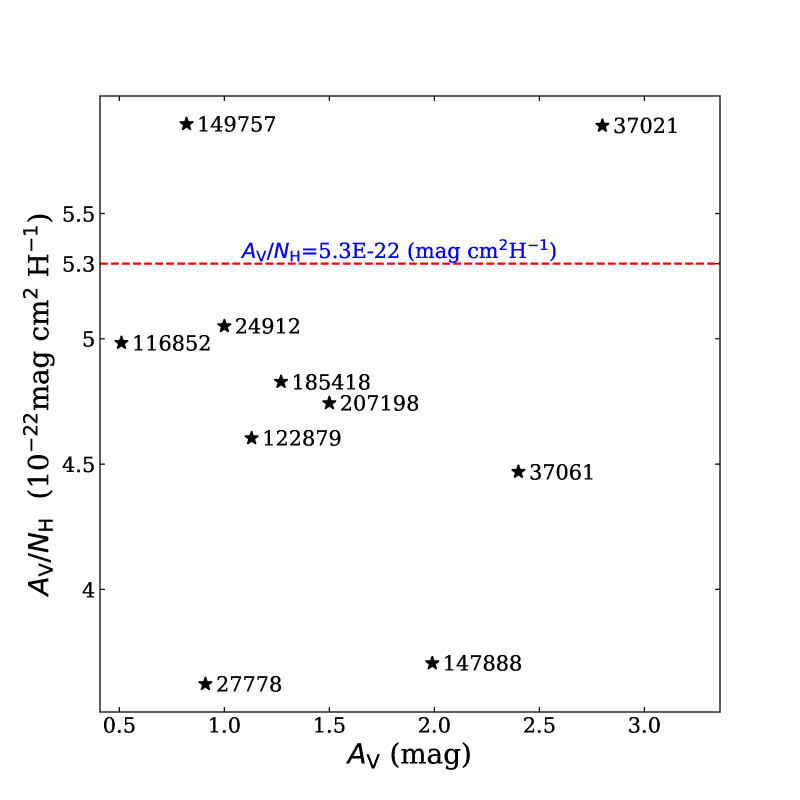
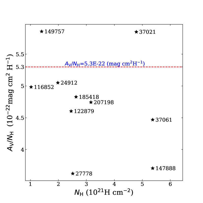
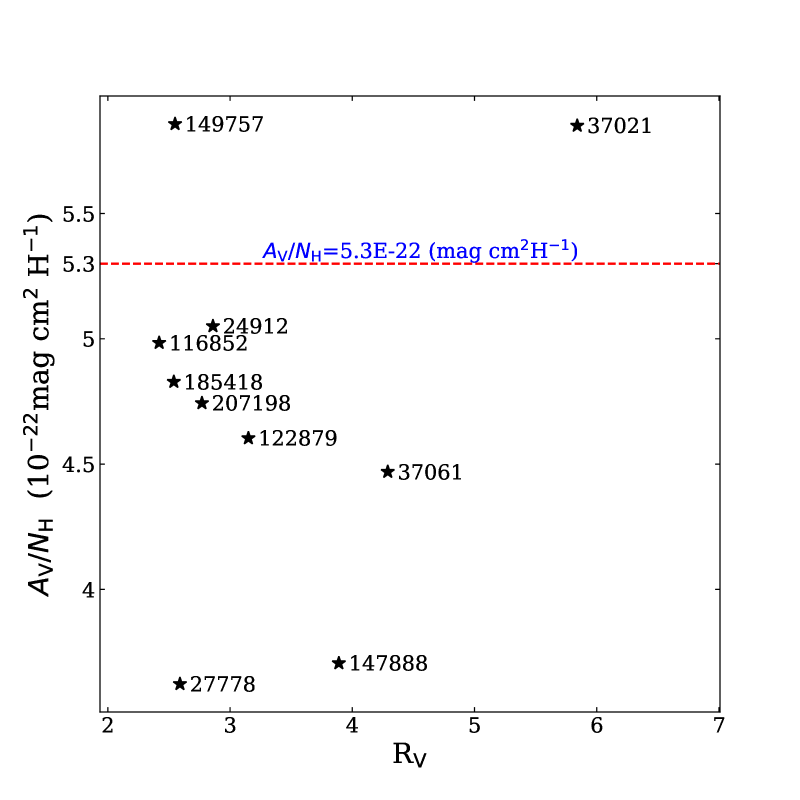
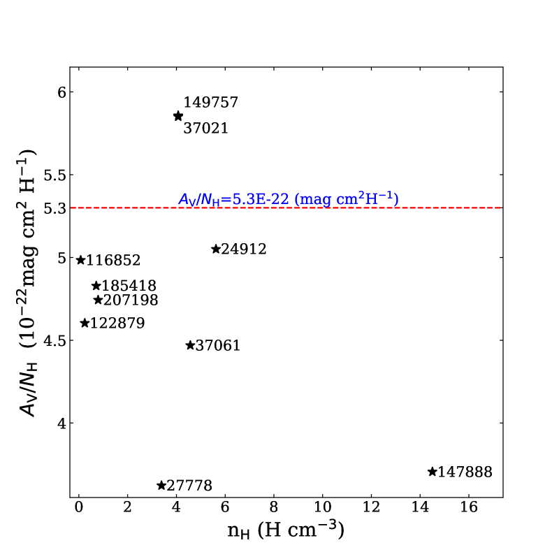
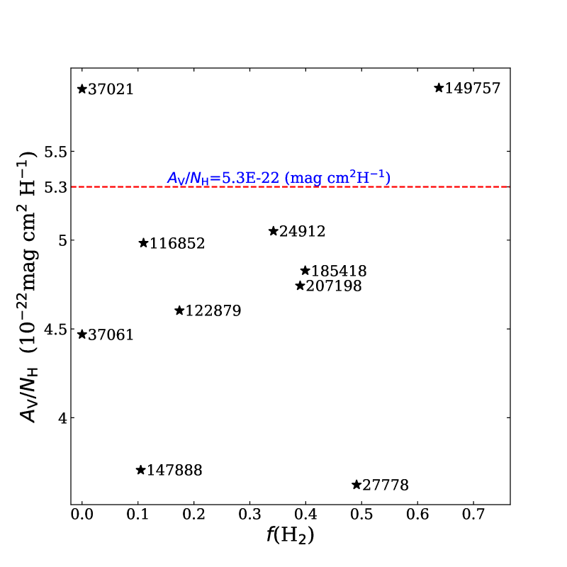
Figure 12: Relations of the ratio of visual extinction to hydrogen column density (${A_{V}}/N_{\rm H}$) with the visual extinction (${A_{V}}$; panel a), the total-to-selective extinction ratio (${R_{V}}$; panel b), the hydrogen column density ($N_{\rm H}$; panel c), the hydrogen volume density ($n_{\rm H}$; panel d), and the molecular hydrogen fraction [$f({\rm H}_{2})\equiv 2N({\rm H_{2}})/\left\{N({\rm HI})+2N({\rm H_{2}})\right\}$, panel e]. The dashed horizontal line shows the canonical ratio of ${A_{V}}/N_{\rm H}=5.3\times 10^{-23}\,{\rm mag}\,{\rm cm}^{2}\,{\rm H}^{-1}$.

We have also explored the relationships between ${A_{V}}/N_{\rm H}$ and the physical and chemical conditions of the interstellar environments, including ${A_{V}}$, ${R_{V}}$, $N_{\rm H}$, $\langle n_{\rm H}\rangle$, and $f({\rm H}_{2})\equiv 2N({\rm H_{2}})/\left\{N({\rm HI})+2N({\rm H_{2}})\right\}$, the fraction of molecular hydrogen in the line of sight (see Figure 12). For the 10 lines of sight considered here, ${A_{V}}/N_{\rm H}$ does not appear to show any appreciable correlations with these parameters. This seems to contradict the conventional belief that, due to grain aggregation (e.g., see Jura 1980), ${A_{V}}/N_{\rm H}$ decreases toward denser regions which are often characterized by larger values of ${R_{V}}$, $\langle n_{\rm H}\rangle$, and $f({\rm H}_{2})$. Kim & Martin (1996) explored the variation of ${A_{V}}/N_{\rm H}$ with ${R_{V}}$ for several dozen sightlines spanning $2.7<{R_{V}}<5.6$. Despite a large scatter, they found a somewhat increase of ${A_{V}}/N_{\rm H}$ with ${R_{V}}$ for ${R_{V}}<4.4$, and above this value, ${A_{V}}/N_{\rm H}$ tends to be smaller. With ${R_{V}}\approx 2.1$, the high Galactic latitude cloud toward HD 210121 has ${A_{V}}/N_{\rm H}\approx 4.2\times 10^{-22}\,{\rm mag}\,{\rm cm}^{2}\,{\rm H}^{-1}$ (see Li & Greenberg 1998), about 20% lower than that of the canonical value of ${A_{V}}/N_{\rm H}\approx 5.3\times 10^{-22}\,{\rm mag}\,{\rm cm}^{2}\,{\rm H}^{-1}$ (Bohlin et al. 1978).

6 Summary

We have compiled a “gold” sample of 10 lines of sight for which the extinction parameters and the gas-phase abundances of the dust-forming elements C, O, Si, Mg and Fe have been observationally determined. We have applied the KK relation to this sample to examine the viability of (i) the abundances of B stars, (ii) the solar, (iii) protosolar and (iv) GCE-augmented solar abundances as the interstellar reference abundances. Except that we assume the ISM is made of either (i) graphite and Fe-containing amorphous silicates, or (ii) graphite and Fe-lacking amorphous silicates plus iron oxides, or (iii) graphite and Fe-lacking amorphous silicates plus iron, our approach is model-independent in the sense that we do not need to specify the dust size distritbution and do not need to reproduce the observed extinction curves. Our principal results are as follows:

1. For each of the (10) lines of sight, each of the (four) assumed sets of interstellar reference abundances and each of the (three) assumed different dust mixtures, we have calculated the dust volumes and the KK-based wavelength-integrated extinction. We have also calculated the observation-based wavelength-integrated extinction for each sightline. We have found that only the GCE-augmented protosolar abundances could meet the KK criterion that the former must exceed the latter.

2. Although we have assumed the interstellar carbonaceous dust component to be graphite, the exact composition of this component (e.g., amorphous carbon vs. graphite) is not critical. Also, although we have assumed interstellar dust to be a mixture of separate, distinct individual dust species, the exact dust structural form (e.g., core-mantle or composite) does not affect our conclusion.

3. For this sample we have investigated the “missing O” problem (i.e., in the diffuse ISM a substantial fraction of the O/H remains unaccounted for in interstellar atoms, molecules and dust) and found that for the majority of the lines of sight the ISM does not seem to have difficulty in accommodating the O atoms.

4. For this sample we have derived the extinction-to-hydrogen gas ratio to be ${A_{V}}/N_{\rm H}\approx 4.6\times 10^{-22}\,{\rm mag}\,{\rm cm}^{2}\,{\rm H}^{-1}$, $\sim\,$13% lower than the canonical value of ${A_{V}}/N_{\rm H}\approx 5.3\times 10^{-22}\,{\rm mag}\,{\rm cm}^{2}\,{\rm H}^{-1}$. Also, ${A_{V}}/N_{\rm H}$ does not systematically decrease toward denser regions as indicated by larger values of ${R_{V}}$, hydrogen volume density $\langle n_{\rm H}\rangle$, and molecular fraction of hydrogen $f({\rm H}_{2})$, contrary to the conventional wisdom of more reduced ${A_{V}}/N_{\rm H}$ in denser regions due to grain coagulation.

Table 1: Solar and stellar abundances as plausible interstellar reference abundances for the dust-forming elements (relative to 10⁶ H atoms).

Element	B starsa	Solarb	Solarc	Protosolard	GCE-augmented protosolare
C	$209\pm 15$	$363\pm 33$	$269\pm 31$	$288\pm 27$	$339\pm 39$
O	$575\pm 40$	$851\pm 69$	$490\pm 57$	$575\pm 66$	$589\pm 68$
Mg	$36.3\pm 4.2$	$38.0\pm 4.4$	$39.8\pm 3.7$	$41.7\pm 1.9$	$47.9\pm 4.4$
Si	$31.6\pm 1.5$	$35.5\pm 4.1$	$32.4\pm 2.2$	$40.7\pm 1.9$	$42.7\pm 4.0$
Fe	$27.5\pm 2.5$	$46.8\pm 3.2$	$31.6\pm 2.9$	$34.7\pm 2.4$	$47.9\pm 4.4$

(a) Przybilla et al. (2008); (b) Anders & Grevesse (1989); (c) Asplund et al. (2009); (d) Lodders (2003); (e) Protosolar abundances augmented by GCE (Asplund et al. 2009, Chiappini et al. 2003).

Table 2: Gas Column Densities and Abundances of the Ten Interstellar Lines of Sight in the “Gold” Sample

Star	$N_{\rm H}$	$N({\rm HI})$	$N({\rm H_{2}})$	$\left[{\rm C/H}\right]_{\rm gas}$	$\left[{\rm O/H}\right]_{\rm gas}$	$\left[{\rm S/H}\right]_{\rm gas}$	$\left[{\rm Mg/H}\right]_{\rm gas}$	$\left[{\rm Si/H}\right]_{\rm gas}$	$\left[{\rm Fe/H}\right]_{\rm gas}$
	($10^{21}\,{\rm cm}^{-2}$)	($10^{21}\,{\rm cm}^{-2}$)	($10^{21}\,{\rm cm}^{-2}$)	(ppm)	(ppm)	(ppm)	(ppm)	(ppm)	(ppm)
HD 24912	1.98$\pm$0.54 (2)	1.20$\pm$0.18 (3)	0.34$\pm$0.07 (3)	163.1$\pm$86.5 (16)	326.1$\pm$97.5 (3)	1.75$\pm$0.48 (4)	1.99$\pm$0.17 (2)	1.61$\pm$0.44 (2)	0.92$\pm$0.25 (13)
HD 27778	2.51$\pm$0.44 (7)	0.89 (5)	0.62 (10)	79.2$\pm$27.6 (14)	269.2$\pm$ 53.8 (3)	–	1.05$\pm$0.22 (7)	3.43$\pm$ 0.60 (9)	0.10$\pm$0.018 (9)
HD 37021	4.79$\pm$1.50 (3)	4.79$\pm$1.50 (3)	–	90.9$\pm$37.9 (14)	257.0$\pm$82.6 (3)	–	1.78$\pm$0.57 (7)	2.99$\pm$1.15 (9)	0.58$\pm$0.19 (9)
HD 37061	5.37$\pm$1.20 (3)	5.37$\pm$1.20 (3)	–	98.1$\pm$35.5 (14)	316.2$\pm$72.2 (3)	0.38$\pm$17.9 (4)	1.12$\pm$0.26 (7)	0.20$\pm$0.17 (4)	0.06$\pm$0.08 (4)
HD 116852	1.02$\pm$0.09 (1)	0.91$\pm$0.08 (1)	0.06${}^{+0.012}_{-0.009}$ (1)	117.3$\pm$103.2 (15)	537.5$\pm$133.2 (1)	3.89$\pm$27.4 (4)	7.76$\pm$0.74 (1)	2.57$\pm$0.39 (4)	0.98$\pm$0.35 (4)
HD 122879	2.45${}^{+0.28}_{-0.23}$ (1)	2.04${}^{+0.28}_{-0.24}$ (1)	0.21${}^{+0.04}_{-0.03}$ (1)	324.3$\pm$38.2 (15)	448.1$\pm$72.8 (1)	–	6.44$\pm$0.76 (1)	4.97$\pm$0.61 (2)	0.53$\pm$0.10 (6)
HD 147888	5.37${}^{+0.87}_{-2.10}$ (1)	4.79${}^{+0.88}_{-2.10}$ (1)	0.28${}^{+0.03}_{-0.05}$ (1)	105.4$\pm$22.6 (14)	301.7$\pm$50.6 (1)	0.49$\pm$0.33 (4)	1.86$\pm$0.33 (1)	2.44$\pm$0.60 (9)	0.15$\pm$0.08 (6)
HD 149757	1.40$\pm$0.03 (2)	0.51$\pm$0.02 (3)	0.45$\pm$0.06 (3)	100.9$\pm$48.6 (11)	307.1$\pm$29.1 (8)	2.37$\pm$4.14 (4)	1.86$\pm$0.16 (2)	1.50$\pm$0.04 (2)	0.32$\pm$0.09 (4)
HD 185418	2.63${}^{+0.24}_{-0.18}$ (1)	1.55${}^{+0.18}_{-0.14}$ (1)	0.53${}^{+0.09}_{-0.07}$ (1)	167.7$\pm$22.8 (15)	380.2$\pm$43.8 (1)	0.87$\pm$ 0.08 (12)	4.07$\pm$0.42 (1)	0.060$\pm$0.01 (12)	0.32$\pm$0.09 (12)
HD 207198	3.16${}^{+0.36}_{-0.44}$ (1)	1.91${}^{+0.31}_{-0.40}$ (1)	0.62$\pm$0.07 (1)	102.1$\pm$25.1 (14)	445.9$\pm$59.9 (1)	1.20$\pm$20.2 (4)	3.64$\pm$0.43 (1)	2.19$\pm$1.07 (9)	0.43$\pm$0.08 (9)

(1) Jenkins (2019); (2) Gnaciński et al. (2006); (3) Cartledge et al. (2004); (4) van Steenberg et al. (1988); (5) Welty et al. (2010); (6) Jensen et al. (2007a); (7) Jensen et al. (2007b); (8) Knauth et al. (2006); (9) Miller et al. (2007); (10) Sheffer et al. (2007); (11) Sofia et al. (1994); (12) Sonnentrucker et al. (2003); (13) Jenkins et al. (1986); (14) Sofia et al. (2011); (15) Parvathi et al. (2012); (16) Sofia et al. (2004).

Table 3: Extinction Parameters of the Ten Interstellar Lines of Sight in the Gold Sample

Star	${A_{U}}$b	${A_{B}}$b	${A_{V}}$a	${A_{J}}$b	${A_{H}}$b	${A_{K}}$b	$E(B-V)$a	${R_{V}}$a	$c_{1}^{\prime}$a	$c_{2}^{\prime}$a	$c_{3}^{\prime}$a	$c_{4}^{\prime}$a	$x_{0}$a	$\gamma$a
	(mag)	(mag)	(mag)	(mag)	(mag)	(mag)	(mag)						($\mu{\rm m}^{-1}$)	($\mu{\rm m}^{-1}$)
HD 24912	–	–	1.00$\pm$0.21	–	–	–	0.35$\pm$0.04	2.86$\pm$0.51	1.187$\pm$0.728	0.270$\pm$0.054	0.943$\pm$0.219	0.050$\pm$0.024	4.541$\pm$0.016	0.846$\pm$0.028
HD 277781	1.58	1.25	0.91$\pm$0.14	0.19	0.11	0.07	0.35$\pm$0.04	2.59$\pm$0.24	1.421$\pm$0.252	0.232$\pm$0.038	0.878$\pm$0.180	0.386$\pm$0.062	4.603$\pm$0.012	0.974$\pm$0.032
HD 37021	–	–	2.80$\pm$0.17	–	–	–	0.48$\pm$0.02	5.84$\pm$0.26	1.063$\pm$1.047	0.020$\pm$0.008	0.235$\pm$0.043	0.007$\pm$0.007	4.584$\pm$0.047	1.081$\pm$0.036
HD 370611	3.33	2.93	2.40$\pm$0.21	0.72	0.45	0.3	0.56$\pm$0.04	4.29$\pm$0.21	1.544$\pm$0.145	0.000$\pm$0.100	0.310$\pm$0.042	0.050$\pm$0.012	4.574$\pm$0.014	0.901$\pm$0.029
HD 116852	–	–	0.51$\pm$0.12	–	–	–	0.21$\pm$0.04	2.42$\pm$0.37	0.518$\pm$0.249	0.376$\pm$0.103	0.633$\pm$0.173	0.010$\pm$0.015	4.548$\pm$0.041	0.782$\pm$0.069
HD 122879 2	1.69	1.45	1.13$\pm$0.20	–	–	–	0.36$\pm$0.05	3.15$\pm$0.30	1.321$\pm$0.299	0.233$\pm$0.040	1.243$\pm$0.230	0.190$\pm$0.039	4.581$\pm$0.004	0.831$\pm$0.021
HD 147888 1	2.85	2.48	1.99$\pm$0.18	0.6	0.35	0.22	0.51$\pm$0.04	3.89$\pm$0.20	1.471$\pm$0.267	0.037$\pm$ 0.012	0.665 $\pm$0.100	0.087$\pm$0.022	4.587$\pm$0.013	0.879$\pm$0.029
HD 149757 1	1.26	1.09	0.82$\pm$0.13	0.27	0.14	0.1	0.32$\pm$0.04	2.55$\pm$0.24	1.002$\pm$0.100	0.286$\pm$0.037	1.872$\pm$0.313	0.215$\pm$0.052	4.552$\pm$0.010	1.186$\pm$0.042
HD 185418 1	2.07	1.78	1.27$\pm$0.14	0.21	0.11	0.07	0.50$\pm$0.04	2.54$\pm$0.20	1.817$\pm$0.265	0.100$\pm$0.018	1.156$\pm$0.170	0.158$\pm$0.029	4.604$\pm$0.005	0.819$\pm$0.024
HD 207198 2	2.43	1.96	1.50$\pm$0.29	–	–	–	0.54$\pm$0.08	2.77$\pm$0.35	0.811$\pm$0.259	0.344$\pm$0.050	0.976$\pm$0.169	0.277$\pm$0.045	4.596$\pm$0.006	0.883$\pm$0.024

Table 4: Wavelength-Integrated Extinction Obtained from the Observed Extinction Curves [$A_{\rm int}^{\rm obs}(\rm\scriptsize WD)$ and $A_{\rm int}^{\rm obs}(\rm\scriptsize WLJ)$] and from the Dust Volumes Based on the KK Relation [$A_{\rm int}^{\rm\scriptsize KK}$]. The Dust Volumes Are Derived from the Assumption of the Abundances of B Stars as the Interstellar Reference Abundances and the Dust as Mixtures of (i) Graphite + Fe-Containing Amorphous Silicates, (ii) Graphite + Fe-Lacking Amorphous Silicates + Iron Oxides, and (iii) Graphite + Fe-Lacking Amorphous Silicates + Iron.

Star	$A_{\rm int}^{\rm obs}(\rm\scriptsize WD)/N_{\rm H}$1	$A_{\rm int}^{\rm obs}(\rm\scriptsize WLJ)/N_{\rm H}$2	Graphite + Fe-containing Silicate				Graphite + Fe-lacking Silicate + FexOy							Graphite + Fe-lacking Silicate + Fe
			$V_{\rm gra}$/H3	$V_{\rm sil}$/H4	$A_{\rm int}^{\rm\scriptsize KK}/N_{\rm H}$5		$V_{\rm gra}$/H3	$V_{\rm sil}$/H6	$V_{\rm FeO}$/H7	$V_{\rm Fe_{2}O_{3}}$/H8	$V_{\rm Fe_{3}O_{4}}$/H9	$A_{\rm int}^{\rm\scriptsize KK}/N_{\rm H}$5		$V_{\rm gra}$/H3	$V_{\rm sil}$/H6	$V_{\rm Fe}$/H10	$A_{\rm int}^{\rm\scriptsize KK}/N_{\rm H}$5
HD 24912	1.24E-25	1.52E-25	1.51E-28	2.29E-27	7.41E-26		1.51E-28	1.73E-27	1.86E-28	2.24E-28	2.20E-28	7.46E-26		1.51E-28	1.74E-27	3.17E-28	6.46E-26
HD 27778	9.07E-26	1.10E-25	1.15E-27	2.25E-27	1.22E-25		1.15E-27	1.67E-27	1.91E-28	2.31E-28	2.26E-28	1.23E-25		1.15E-27	1.67E-27	3.27E-28	1.13E-25
HD 37021	1.42E-25	1.82E-25	1.05E-27	2.25E-27	1.17E-25		1.05E-27	1.68E-27	1.88E-28	2.27E-28	2.22E-28	1.18E-25		1.05E-27	1.68E-27	3.21E-28	1.07E-25
HD 37061	1.07E-25	1.35E-25	9.86E-28	2.38E-27	1.17E-25		9.86E-28	1.81E-27	1.92E-28	2.31E-28	2.27E-28	1.18E-25		9.86E-28	1.81E-27	3.27E-28	1.08E-25
HD 116852	1.24E-25	1.50E-25	8.16E-28	2.19E-27	1.03E-25		8.16E-28	1.62E-27	1.85E-28	2.23E-28	2.19E-28	1.04E-25		8.16E-28	1.62E-27	3.16E-28	9.43E-26
HD 122879	1.15E-25	1.42E-25	–	2.12E-27	6.16E-26		–	1.53E-27	1.89E-28	2.27E-28	2.23E-28	6.28E-26		–	1.53E-27	3.21E-28	5.26E-26
HD 147888	8.96E-26	1.13E-25	9.21E-28	2.28E-27	1.11E-25		9.21E-28	1.70E-27	1.91E-28	2.30E-28	2.26E-28	1.12E-25		9.21E-28	1.70E-27	3.26E-28	1.02E-25
HD 149757	1.47E-25	1.77E-25	9.62E-28	2.31E-27	1.14E-25		9.62E-28	1.74E-27	1.90E-28	2.29E-28	2.25E-28	1.15E-25		9.62E-28	1.74E-27	3.24E-28	1.05E-25
HD 185418	1.16E-25	1.41E-25	3.68E-28	2.35E-27	8.62E-26		3.68E-28	1.78E-27	1.90E-28	2.29E-28	2.24E-28	8.68E-26		3.68E-28	1.78E-27	3.24E-28	7.66E-26
HD 207198	1.22E-25	1.48E-25	9.50E-28	2.26E-27	1.12E-25		9.50E-28	1.69E-27	1.89E-28	2.28E-28	2.24E-28	1.13E-25		9.50E-28	1.69E-27	3.23E-28	1.03E-25

${1}$

$A_{\rm int}^{\rm obs}(\rm\scriptsize WD)/N_{\rm H}$ (mag$\,{\rm cm}^{3}$ H^-1) is the observed extinction (per H column) integrated from 912$\,{\rm\AA}$ to 1$\,{\rm cm}$, with the extinction at $0.9<\lambda<1\,{\rm cm}$ approximated by the ${R_{V}}=3.1$ model curve of Weingartner & Draine (2001);

${2}$

$A_{\rm int}^{\rm obs}(\rm\scriptsize WLJ)/N_{\rm H}$ (mag$\,{\rm cm}^{3}$ H^-1) is the observed extinction (per H column) integrated from 912$\,{\rm\AA}$ to 1$\,{\rm cm}$, with the extinction at $0.9<\lambda<1\,{\rm cm}$ approximated by the ${R_{V}}=3.1$ model curve of Wang, Li & Jiang (2015a);

${3}$

$V_{\rm gra}/{\rm H}$ (cm³ H^-1) is the volume (per H nucleon) of graphite grains;

${4}$

$V_{\rm sil}/{\rm H}$ (cm³ H^-1) is the volume (per H nucleon) of Fe-containing amorphous silicate grains;

${5}$

$A_{\rm int}^{\rm\scriptsize KK}/N_{\rm H}$ (mag$\,{\rm cm}^{3}$ H^-1) is the KK-based wavelength-integrated extinction derived from the dust volumes;

${6}$

$V_{\rm sil}/{\rm H}$ (cm³ H^-1) is the volume (per H nucleon) of Fe-lacking amorphous silicate grains;

${7}$

$V_{\rm FeO}/{\rm H}$ (cm³ H^-1) is the volume (per H nucleon) of FeO grains;

${8}$

$V_{\rm Fe_{2}O_{3}}/{\rm H}$ (cm³ H^-1) is the volume (per H nucleon) of Fe₂O₃ grains;

${9}$

$V_{\rm Fe_{3}O_{4}}/{\rm H}$ (cm³ H^-1) is the volume (per H nucleon) of Fe₃O₄ grains;

${10}$

$V_{\rm Fe}/{\rm H}$ (cm³ H^-1) is the volume (per H nucleon) of iron grains.

Table 5: Same as Table 4 but with the Solar Abundances as the Interstellar Reference Abundances.

Star	$A_{\rm int}^{\rm obs}(\rm\scriptsize WD)/N_{\rm H}$	$A_{\rm int}^{\rm obs}(\rm\scriptsize WLJ)/N_{\rm H}$	Graphite + Fe-containing Silicate				Graphite + Fe-lacking Silicate + FexOy							Graphite + Fe-lacking Silicate + Fe
			$V_{\rm gra}$/H	$V_{\rm sil}$/H	$A_{\rm int}^{\rm\scriptsize KK}/N_{\rm H}$		$V_{\rm gra}$/H	$V_{\rm sil}$/H	$V_{\rm FeO}$/H	$V_{\rm Fe_{2}O_{3}}$/H	$V_{\rm Fe_{3}O_{4}}$/H	$A_{\rm int}^{\rm\scriptsize KK}/N_{\rm H}$		$V_{\rm gra}$/H	$V_{\rm sil}$/H	$V_{\rm Fe}$/H	$A_{\rm int}^{\rm\scriptsize KK}/N_{\rm H}$
HD 24912	1.24E-25	1.52E-25	9.41E-28	2.47E-27	1.18E-25		9.41E-28	1.81E-27	2.14E-28	2.58E-28	2.53E-28	1.19E-25		6.85E-28	1.81E-27	3.66E-28	1.08E-25
HD 27778	9.07E-26	1.10E-25	1.69E-27	2.43E-27	1.53E-25		1.69E-27	1.74E-27	2.20E-28	2.65E-28	2.60E-28	1.55E-25		1.69E-27	1.74E-27	3.75E-28	1.43E-25
HD 37021	1.42E-25	1.82E-25	1.58E-27	2.43E-27	1.48E-25		1.58E-27	1.76E-27	2.17E-28	2.61E-28	2.56E-28	1.49E-25		1.58E-27	1.76E-27	3.70E-28	1.38E-25
HD 37061	1.07E-25	1.35E-25	1.52E-27	2.56E-27	1.49E-25		1.52E-27	1.88E-27	2.20E-28	2.65E-28	2.61E-28	1.50E-25		1.52E-27	1.88E-27	3.76E-28	1.38E-25
HD 116852	1.24E-25	1.50E-25	1.35E-27	2.37E-27	1.35E-25		1.35E-27	1.70E-27	2.14E-28	2.58E-28	2.53E-28	1.36E-25		1.35E-27	1.70E-27	3.65E-28	1.25E-25
HD 122879	1.15E-25	1.42E-25	–	2.30E-27	6.69E-26		–	1.61E-27	2.17E-28	2.62E-28	2.57E-28	6.86E-26		–	1.61E-27	3.70E-28	5.69E-26
HD 147888	8.96E-26	1.13E-25	1.45E-27	2.46E-27	1.43E-25		1.45E-27	1.78E-27	2.20E-28	2.65E-28	2.60E-28	1.44E-25		1.45E-27	1.78E-27	3.75E-28	1.32E-25
HD 149757	1.47E-25	1.77E-25	1.50E-27	2.49E-27	1.46E-25		1.50E-27	1.82E-27	2.19E-28	2.63E-28	2.58E-28	1.47E-25		1.50E-27	1.82E-27	3.73E-28	1.35E-25
HD 185418	1.16E-25	1.41E-25	9.01E-28	2.53E-27	1.18E-25		9.01E-28	1.85E-27	2.19E-28	2.63E-28	2.58E-28	1.19E-25		9.01E-28	1.85E-27	3.73E-28	1.07E-25
HD 207198	1.22E-25	1.48E-25	1.48E-27	2.44E-27	1.44E-25		1.48E-27	1.77E-27	2.18E-28	2.62E-28	2.58E-28	1.45E-25		1.48E-27	1.77E-27	3.72E-28	1.33E-25

Table 6: Same as Table 4 but with the Protosolar Abundances as the Interstellar Reference Abundances.

Star	$A_{\rm int}^{\rm obs}(\rm\scriptsize WD)/N_{\rm H}$	$A_{\rm int}^{\rm obs}(\rm\scriptsize WLJ)/N_{\rm H}$	Graphite + Fe-containing Silicate				Graphite + Fe-lacking Silicate + FexOy							Graphite + Fe-lacking Silicate + Fe
			$V_{\rm gra}$/H	$V_{\rm sil}$/H	$A_{\rm int}^{\rm\scriptsize KK}/N_{\rm H}$		$V_{\rm gra}$/H	$V_{\rm sil}$/H	$V_{\rm FeO}$/H	$V_{\rm Fe_{2}O_{3}}$/H	$V_{\rm Fe_{3}O_{4}}$/H	$A_{\rm int}^{\rm\scriptsize KK}/N_{\rm H}$		$V_{\rm gra}$/H	$V_{\rm sil}$/H	$V_{\rm Fe}$/H	$A_{\rm int}^{\rm\scriptsize KK}/N_{\rm H}$
HD 24912	1.24E-25	1.52E-25	1.11E-27	2.91E-27	1.39E-25		1.11E-27	2.20E-27	2.36E-28	2.84E-28	2.79E-28	1.40E-25		1.11E-27	2.20E-27	4.03E-28	1.27E-25
HD 27778	9.07E-26	1.10E-25	1.86E-27	2.87E-27	1.74E-25		1.86E-27	2.13E-27	2.42E-28	2.91E-28	2.86E-28	1.75E-25		1.86E-27	2.13E-27	4.12E-28	1.62E-25
HD 37021	1.42E-25	1.82E-25	1.75E-27	2.86E-27	1.69E-25		1.75E-27	2.14E-27	2.38E-28	2.87E-28	2.82E-28	1.70E-25		1.75E-27	2.14E-27	4.07E-28	1.57E-25
HD 37061	1.07E-25	1.35E-25	1.69E-27	3.00E-27	1.70E-25		1.69E-27	2.27E-27	2.42E-28	2.91E-28	2.86E-28	1.70E-25		1.69E-27	2.27E-27	4.13E-28	1.57E-25
HD 116852	1.24E-25	1.50E-25	1.52E-27	2.80E-27	1.56E-25		1.52E-27	2.08E-27	2.36E-28	2.84E-28	2.79E-28	1.57E-25		1.52E-27	2.08E-27	4.02E-28	1.44E-25
HD 122879	1.15E-25	1.42E-25	–	2.73E-27	7.95E-26		–	2.00E-27	2.39E-28	2.88E-28	2.82E-28	8.08E-26		–	2.00E-27	4.07E-28	6.80E-26
HD 147888	8.96E-26	1.13E-25	1.62E-27	2.90E-27	1.64E-25		1.62E-27	2.16E-27	2.42E-28	2.91E-28	2.85E-28	1.65E-25		1.62E-27	2.16E-27	4.12E-28	1.52E-25
HD 149757	1.47E-25	1.77E-25	1.66E-27	2.93E-27	1.67E-25		1.66E-27	2.20E-27	2.40E-28	2.89E-28	2.84E-28	1.67E-25		1.66E-27	2.20E-27	4.10E-28	1.54E-25
HD 185418	1.16E-25	1.41E-25	1.07E-27	2.96E-27	1.38E-25		1.07E-27	2.24E-27	2.40E-28	2.89E-28	2.84E-28	1.39E-25		1.07E-27	2.24E-27	4.10E-28	1.26E-25
HD 207198	1.22E-25	1.48E-25	1.65E-27	2.88E-27	1.65E-25		1.65E-27	2.15E-27	2.40E-28	2.88E-28	2.83E-28	1.65E-25		1.65E-27	2.15E-27	4.08E-28	1.53E-25

Table 7: Same as Table 4 but with the GCE-augmented Protosolar Abundances as the Interstellar Reference Abundances.

Star	$A_{\rm int}^{\rm obs}(\rm\scriptsize WD)/N_{\rm H}$	$A_{\rm int}^{\rm obs}(\rm\scriptsize WLJ)/N_{\rm H}$	Graphite + Fe-containing Silicate				Graphite + Fe-lacking Silicate + FexOy							Graphite + Fe-lacking Silicate + Fe
			$V_{\rm gra}$/H	$V_{\rm sil}$/H	$A_{\rm int}^{\rm\scriptsize KK}/N_{\rm H}$		$V_{\rm gra}$/H	$V_{\rm sil}$/H	$V_{\rm FeO}$/H	$V_{\rm Fe_{2}O_{3}}$/H	$V_{\rm Fe_{3}O_{4}}$/H	$A_{\rm int}^{\rm\scriptsize KK}/N_{\rm H}$		$V_{\rm gra}$/H	$V_{\rm sil}$/H	$V_{\rm Fe}$/H	$A_{\rm int}^{\rm\scriptsize KK}/N_{\rm H}$
HD 24912	1.24E-25	1.52E-25	1.56E-27	3.41E-27	1.76E-25		1.56E-27	2.36E-27	3.28E-28	3.95E-28	3.88E-28	1.78E-25		1.56E-27	2.36E-27	5.60E-28	1.61E-25
HD 27778	9.07E-26	1.10E-25	2.31E-27	3.37E-27	2.11E-25		2.31E-27	2.29E-27	3.34E-28	4.02E-28	3.95E-28	2.14E-25		2.31E-27	2.29E-27	5.70E-28	1.96E-25
HD 37021	1.42E-25	1.82E-25	2.21E-27	3.36E-27	2.06E-25		2.21E-27	2.30E-27	3.31E-28	3.98E-28	3.91E-28	2.09E-25		2.21E-27	2.30E-27	5.64E-28	1.91E-25
HD 37061	1.07E-25	1.35E-25	2.14E-27	3.50E-27	2.06E-25		2.14E-27	2.43E-27	3.34E-28	4.03E-28	3.95E-28	2.09E-25		2.14E-27	2.43E-27	5.70E-28	1.91E-25
HD 116852	1.24E-25	1.50E-25	1.97E-27	3.30E-27	1.92E-25		1.97E-27	2.25E-27	3.28E-28	3.95E-28	3.88E-28	1.96E-25		1.97E-27	2.25E-27	5.59E-28	1.78E-25
HD 122879	1.15E-25	1.42E-25	1.31E-28	3.23E-27	1.00E-25		1.31E-28	2.16E-27	3.31E-28	3.99E-28	3.91E-28	1.04E-25		1.31E-28	2.16E-27	5.65E-28	8.60E-26
HD 147888	8.96E-26	1.13E-25	2.08E-27	3.40E-27	2.00E-25		2.08E-27	2.33E-27	3.34E-28	4.02E-28	3.94E-28	2.03E-25		2.08E-27	2.33E-27	5.69E-28	1.85E-25
HD 149757	1.47E-25	1.77E-25	2.12E-27	3.43E-27	2.03E-25		2.12E-27	2.37E-27	3.33E-28	4.00E-28	3.93E-28	2.06E-25		2.12E-27	2.37E-27	5.67E-28	1.88E-25
HD 185418	1.16E-25	1.41E-25	1.52E-27	3.46E-27	1.75E-25		1.52E-27	2.40E-27	3.33E-28	4.00E-28	3.93E-28	1.78E-25		1.52E-27	2.40E-27	5.67E-28	1.60E-25
HD 207198	1.22E-25	1.48E-25	2.11E-27	3.38E-27	2.01E-25		2.11E-27	2.32E-27	3.32E-28	4.00E-28	3.92E-28	2.04E-25		2.11E-27	2.32E-27	5.66E-28	1.86E-25

Table 8: Properties of Dust Materials

Candidate	Mass Density	Static Dielectic Constant	$F(a/b;\varepsilon_{0}$)
Dust Material	$\rho$ (g$\,{\rm cm}^{-3}$)	($\varepsilon_{0}$)	Prolate ($a/b=3$)	Oblate ($a/b=1/2$)
Forsterite (Mg2SiO4)	3.27a	5.5a	0.668	0.633
Enstatite (MgSiO3)	3.2b	6.7b	0.749	0.698
Olivine (MgFeSiO4)	3.5a	10a	0.905	0.814
Wüstite (FeO)	5.7c	24c	1.18	0.989
Haematite ($\alpha$-Fe2O3)	5.26d	16e	1.07	0.920
Magnetite (Fe3O4)	5.18d	$\infty$	1.52	1.15
Iron (Fe)	7.8	$\infty$	1.52	1.15
Graphite (C)	2.24	$\infty$	1.52	1.15

(a) Jäger et al. (2003); (b) Dorschner et al. (1995); (c) Henning & Mutschke (1997); (d) Schrettle et al. (2012); (e) Steyer (1974).

References

- (1) Aiello, S., Barsella, B., Chlewicki, G., et al. 1988, A&AS, 73, 195
- (2) Anders, E., & Grevesse, N. 1989, Geochim. Cosmochim. Acta, 53, 197
- (3) Asplund, M., et al. 2009, ARA&A, 47, 481
- (4) Bohlin, R. C., Savage, B. D., & Drake, J. F. 1978, ApJ, 224, 132
- (5) Cardelli, J. A., Clayton, G., C., & Mathis, J. S. 1989, ApJ, 345, 245
- (6) Cardelli, J. A., Meyer, D. M., Jura, M., et al. 1996, ApJ, 467, 334
- (7) Cartledge, S. I. B., Lauroesch, J. T., Meyer, D. M., & Sofia, U. J. 2004, ApJ, 613, 1037
- (8) Cartledge, S. I. B., Meyer, D. M., Lauroesch, J. T., et al. 2001, ApJ, 562, 394
- (9) Chiappini, C., et al. 2003, MNRAS, 339, 63
- (10) Désert, F.-X., Boulanger, F., & Puget, J. L. 1990, A&A, 237, 215
- (11) Diplas, A., & Savage, B.D. 1994, ApJS, 93, 211
- (12) Dorschner, J., Begemann, B., Henning, Th., et al. 1995, A&A, 300, 503
- (13) Draine, B.T. 1989, in IAU Symp. 135, Interstellar Dust, ed. L. J. Allamandola & A. G. G. M. Tielens (Dordrecht: Kluwer), 313
- (14) Draine, B.T. 2015, IAUGA, 29, 2253136
- (15) Draine, B. T., & Hensley, B. 2013, ApJ, 765, 159
- (16) Draine, B. T., & Hensley, B. 2020, arXiv:2009.11314
- (17) Draine, B. T., & Lazarian, A. 1999, ApJ, 512, 740
- (18) Draine, B.T., & Lee, H.M. 1984, ApJ, 258, 89D
- (19) Dwek, E. 2016, ApJ, 825, 136
- (20) Fitzpatrick, E.L., & Massa, D. 1990, ApJS, 72, 163
- (21) Fitzpatrick, E.L., & Massa, D. 2007, ApJ, 663, 320
- (22) Flaherty, K. M., Pipher, J. L., Megeath, S. T., et al. 2007, ApJ, 663,1069
- (23) Forrest, W. J., Houck, J. R., & McCarthy, J. F. 1981, ApJ, 248, 195
- (24) Gao, J., Jiang, B. W., & Li, A. 2009, ApJ, 707,89
- (25) Greenberg, J.M., & Li, A. 1996, A&A, 309, 258
- (26) Gnaciński, P., & Krogulec, M. 2006, Acta Astron., 56, 373
- (27) Gordon, K.D., Cartledge, S., & Clayton, G.C. 2009, ApJ, 705, 1320
- (28) Haris, U., Parvathi, V. S., Gudennavar, S. B., et al. 2016, AJ, 151, 143
- (29) Henning, Th. 2010, ARA&A, 48, 21
- (30) Henning, Th., & Mutschke, H. 1997, A&A, 327, 743
- (31) Henning, Th., & Salama, F. 1998, Science, 282, 2204H
- (32) Hensley, B. S., & Draine, B. T. 2017, ApJ, 836, 179
- (33) Hensley, B. S., & Draine, B. T. 2020a, ApJ, 895, 38
- (34) Hensley, B. S., & Draine, B.T. 2020b, arXiv:2009.00018
- (35) Hildebrand, R.H., & Dragovan, M. 1995, ApJ, 450, 663
- (36) Howell, D. A. 2011, Nature Communications, 2, 350
- (37) Indebetouw, R., Mathis, J. S., Babler, B. L., et al. 2005, ApJ, 619, 931
- (38) Jäger, C., Mutschke, H., & Henning, Th. 1998, A&A, 332, 291
- (39) Jäger, C., Il’in, V. B., Henning, Th., et al. 2003, JQSRT, 79-80, 765
- (40) Jana, R., Nath, B., & Biermann, P. L. 2019, MNRAS, 483, 5329
- (41) Jenkins, E.B. 2009, ApJ, 700, 1299
- (42) Jenkins, E.B. 2019, ApJ, 872, 55
- (43) Jenkins, E. B., Savage, B. D., & Spitzer, L. 1986, ApJ, 301, 355
- (44) Jensen, A. G., Rachford, B. L., & Snow, T. P. 2005, ApJ, 619, 891
- (45) Jensen, A. G., & Snow, T. P. 2007a, ApJ, 669, 378
- (46) Jensen, A. G., & Snow, T. P. 2007b, ApJ, 669, 401
- (47) Jensen, A. G., Snow, T. P., Sonneborn, G., et al. 2010, ApJ, 711, 1236
- (48) Jiang, B. W., Gao, J., Omont, A., et al. 2006, A&A, 446, 551
- (49) Jones, A. P., Duley, W. W., & Williams, D.A. 1990, QJRAS, 31, 567
- (50) Jura, M. 1980, ApJ, 235, 63
- (51) Kim, S.-H., & Martin, P. G. 1996, ApJ, 462, 296
- (52) Knauth, D. C., Meyer, D. M., & Lauroesch, J. T. 2006, ApJ, 647, L115
- (53) Lee, H.M., & Draine, B.T. 1985, ApJ, 290, 211
- (54) Lenz, D., Hensley, B. S., & Doré, O. 2017, ApJ, 846, 38
- (55) Li, A. 2005, ApJ, 622, 965
- (56) Li, A., & Draine, B.T. 2001, ApJ, 554, 778
- (57) Li, A., & Greenberg, J.M. 1997, A&A, 323, 566
- (58) Li, A., & Greenberg, J.M. 1998, A&A, 339, 591
- (59) Li, A., & Greenberg, J.M. 2002, ApJ, 577, 789
- (60) Larson, K. A., Whittet, D. C. B., & Hough, J. H. 1996, ApJ, 472, 755.
- (61) Lodders, K. 2003, ApJ, 591, 1220
- (62) Lutz, D. 1999, in The Universe as Seen by ISO, ed. P. Cox & M. Kessler (ESA Special Publ., Vol. 427; Noordwijk: ESA), 623
- (63) Mathis, J.S., Rumpl, W., & Nordsieck, K.H. 1977, ApJ, 217, 425
- (64) Mathis, J. S. 1996, ApJ, 472, 643
- (65) Meyer, D. M., et al. 1998, ApJ, 493, 222
- (66) Miller, A., Lauroesch, J. T., Sofia, U. J., et al. 2007, ApJ, 659, 441
- (67) Mishra, A., & Li, A. 2015, ApJ, 809, 120
- (68) Mishra, A., & Li, A. 2017, ApJ, 850, 138
- (69) Nieva, M.-F., & Przybilla, N. 2012, A&A, 539, A143
- (70) Nishiyama, S., Tamura, M., Hatano, H., et al. 2009, ApJ, 696, 1407
- (71) Nuth, J. A., Moseley, S. H., Silverberg, R. F., et al. 1985, ApJL, 290, L41
- (72) Parvathi, V. S., Sofia ,U. J., Murthy, J., et al. 2012, ApJ, 760, 36
- (73) Pendleton, Y. J., & Allamandola, L. J. 2002, ApJS, 138, 75
- (74) Poteet, C. A., Whittet, D. C. B., & Draine, B. T. 2015, ApJ, 801, 110
- (75) Potapov, A., Bouwman, J., Jäger, C., et al. 2020, Nature Astronomy, in press
- (76) Poteet, C. A., Whittet, D. C. B., & Draine, B. T. 2015, ApJ, 801, 110
- (77) Przybilla, N., Nieva, M.-F., & Butler, K. 2008, ApJ, 688, L103
- (78) Psaradaki, I., Costantini, E., Mehdipour, M., et al. 2020, arXiv:2009.06244
- (79) Purcell, E. M. 1969, ApJ, 158, 433
- (80) Rogantini, D., Costantini, E., Zeegers, S. T., et al. 2020, arXiv:2007.03329
- (81) Schrettle, F., Kant, C., Lunkenheimer, P., et al. 2012, Eur. Phys. J. B, 85, 164
- (82) Sheffer, Y., Rogers, M., Federman, S. R., et al. 2007, ApJ, 667, 1002
- (83) Snow, T.P., & Witt, A.N. 1995, Science, 270, 1455
- (84) Snow, T.P., & Witt, A.N. 1996, ApJ, 468, L65
- (85) Sofia, U.J., & Meyer, D.M. 2001, ApJ, 554, L221
- (86) Sofia, U. J., Cardelli, J. A., & Savage, B. D. 1994, ApJ, 430, 650
- (87) Sofia, U. J., et al. 1997, ApJ, 482, L105
- (88) Sofia, U. J., Lauroesch, J. T., Meyer, D. M., et al. 2004, ApJ, 605, 272
- (89) Sofia, U. J., Parvathi, V. S., Babu, B. R. S., et al. 2011, AJ, 141, 22
- (90) Sonnentrucker, P., Friedman, S. D., Welty, D. E., et al. 2003, ApJ, 596, 350
- (91) Steyer, T.R. 1974, PhD thesis, Univ. Arizona
- (92) van Steenberg, M. E., & Shull, J. M. 1988, ApJS, 67, 225
- (93) Valencic, L. A., Clayton, G. C., & Gordon, K. D. 2004, ApJ, 616, 912
- (94) Wang, S., Gao, J., Jiang, B.W., Li, A., & Chen, Y. 2013, ApJ, 773, 30
- (95) Wang, S., Li, A., & Jiang, B. W. 2015a, ApJ, 811, 38
- (96) Wang, S., Li, A., & Jiang, B.W. 2015b, MNRAS, 454, 569
- (97) Westphal, A. J., Butterworth, A. L., Tomsick, J. A., et al. 2019, ApJ, 872, 66
- (98) Weingartner, J.C., & Draine, B.T. 2001, ApJ, 548, 296
- (99) Welty, D. E., & Crowther, P. A. 2010, MNRAS, 404, 1321
- (100) White, B., & Sofia, U. J. 2011, BAAS, 43, 129.23
- (101) Whittet, D. C. B., Gerakines, P. A., Hough, J. H., & Shenoy, S. S. 2001a, ApJ, 547, 872
- (102) Whittet, D. C. B., Pendleton, Y. J., Gibb, E. L., et al. 2001b, ApJ, 550, 793
- (103) Whittet, D. C. B. 2010a, LPI Contributions, 1538, 5194
- (104) Whittet, D. C. B. 2010b, ApJ, 710, 1009
- (105) Witt, A. N. 2014, in IAU Symp. 297, The Diffuse Interstellar Bands, ed. J. Cami & N. L. J. Cox (Cambridge: Cambridge Univ. Press), 173
- (106) Witt, A. N., & Vijh, U. P. 2004, in ASP Conf. Ser. 309, Astrophysics of Dust, ed. A.N. Witt, G.C. Clayton, & B.T. Draine (San Francisco: ASP), 115
- (107) Xue, M. Y., Jiang, B. W., Gao, J., et al. 2016, ApJS, 224, 23
- (108) Zhu, H., Tian, W. W., Li, A., & Zhang, M. F. 2017, MNRAS, 471, 3494
- (109) Zubko, V., Dwek, E., & Arendt, R. G. 2004, ApJS, 152, 211